The dwarf galaxy population in nearby clusters from the KIWICS survey

Abstract

We analyse a sample of twelve galaxy clusters, from the Kapteyn IAC WEAVE INT Cluster Survey (KIWICS) looking for dwarf galaxy candidates. By using photometric data in the $r$ and $g$ bands from the Wide Field Camera (WFC) at the 2.5-m Isaac Newton telescope (INT), we select a sample of bright dwarf galaxies (M_r $\leq$ -15.5 mag) in each cluster and analyse their spatial distribution, stellar colour, and as well as their Sérsic index and effective radius. We quantify the dwarf fraction inside the $R_{200}$ radius of each cluster, which ranges from $\sim$ 0.7 to $\sim$ 0.9. Additionally, when comparing the fraction in the inner region with the outermost region of the clusters, we find that the fraction of dwarfs tends to increase going to the outer regions. We also study the clustercentric distance distribution of dwarf and giant galaxies (M_r $<$ -19.0 mag), and in half of the clusters of our sample, the dwarfs are distributed in a statistically different way as the giants, with the giant galaxies being closer to the cluster centre. We analyse the stellar colour of the dwarf candidates and quantify the fraction of blue dwarfs inside the $R_{200}$ radius, which is found to be less than $\sim$ 0.4, but increases with distance from the cluster centre. Regarding the structural parameters, the Sérsic index for the dwarfs we visually classify as early type dwarfs tends to be higher in the inner region of the cluster. These results indicate the role that the cluster environment plays in shaping the observational properties of low-mass halos.

1 Introduction

Galaxy clusters are the largest and gravitationally bound structures in the Universe. They cover a wide range of masses ranging from $\sim$ $10^{12}-10^{15}$ $M_{\odot}$, from small groups with tens of galaxies to clusters with thousands of members, although there is not a sharp line between them. In these high density environments, galaxies evolve under several physical processes that shape their morphology and stellar content. Therefore, galaxy clusters are natural laboratories to study galaxy evolution.

The effect of the environment on galaxy evolution is reflected in different observational properties of field and cluster galaxies. For example, the morphology-density relation (Dressler, 1980), the different structural parameters observed in galaxies in clusters (Aguerri et al., 2004), or the so-called Butcher-Oemler effect (Butcher & Oemler, 1978). These differences between cluster and field galaxies can be explained as consequence of several mechanisms acting in high density environments. Thus, strong tidal interactions between galaxies or with the overall potential of the cluster/group can produce significant transformations among the cluster members (e.g. Moore et al., 1996; Gnedin, 2003; Smith et al., 2015). In addition, the motion of the galaxies through the intracluster medium (or intragroup medium) can remove their cold and hot gas by different processes such as ram-pressure (Quilis et al., 2000; Roman-Oliveira et al., 2019; Cortese et al., 2021), starvation or strangulation (Kawata & Mulchaey, 2008; Fujita, 2004).

Low-mass galaxies are the most abundant in the nearby Universe and within galaxy clusters (Phillipps et al., 1998). They can be divided in two main groups: dwarf ellipticals (dE) and dwarf irregulars (dIrr). The former are characterised by regular shapes and red stellar colours (Kormendy et al., 2009), while dIrr show blue colours and irregular morphologies (e.g. van Zee, 2000). Dwarf galaxies also follow the morphology-density relation. The number of dE increases with the galaxy density (Binggeli et al., 1988; Trentham & Tully, 2002). In contrast, dIrr are mostly found in the outer cluster regions or in field environments (e.g. Sánchez-Janssen et al., 2008; Venhola et al., 2019).

The formation and evolution of dwarf galaxies is still matter of debate, but it is well known that due to their shallow gravitational potential dwarf galaxies are, in general, more susceptible to the environment. Observational evidence suggests that dwarf ellipticals might be the result of galaxy transformations: gas-rich dwarf galaxies can be transformed into dE by the removal of their gas content and the quenching of their star formation. In addition, bright galaxies can lose mass and be transformed into dwarf ones. Several external process related with the environment have been proposed to explain these transformations against the internal effects (see e.g., Boselli & Gavazzi, 2006).

In some nearby clusters a number of environmental transformation processes have been caught in the act. In the Hydra I cluster, Koch et al. (2012) reported an ongoing tidal disruption of a dwarf galaxy, indicating how tidal forces can shape the morphological and kinematic properties of a dwarf galaxy. In a similar way, in the Virgo cluster, Kenney et al. (2014) reported a ram pressure stripping tail in the dIrr galaxy IC34188, a similar tail has been also reported in a dIrr galaxy in the Cen A group (Johnson et al., 2015).

A number of observations support the scenario of the dwarf transformation from gas stripping (e.g. Janz et al., 2021). For instance: $i)$ a similar faint-end slope of the spectroscopic galaxy luminosity function in clusters and field (suggesting that the environment acts to modify the star formation activity; Boselli et al., 2011; Agulli et al., 2014; Aguerri et al., 2020); $ii)$ the relation between gas content, colour and cluster location (Gavazzi et al., 2013); $iii)$ the distribution in some nearby clusters of the dwarf post-starburst galaxies (Aguerri et al., 2018); $iv)$ the relation between age, metallicity and location in the clusters of dwarf galaxies (Boselli et al., 2008; Smith et al., 2009; Toloba et al., 2009; Koleva et al., 2013); $v)$ the presence of blue cores in some early-type dwarfs (Lisker et al., 2007; Pak et al., 2014; Urich et al., 2017; Hamraz et al., 2019). Nevertheless, the family of early-type dwarf galaxies is complex. Their formation might be influenced by different factors rather than a single effect (Hamraz et al., 2019). Some early-type dwarf galaxies show several morphological structures like disk features and blue centres (Aguerri et al., 2005; Lisker et al., 2007; Janz et al., 2014), rotation (Toloba et al., 2009), or the presence of star formation, gas and dust in their centres (Lisker et al., 2006a; Lisker et al., 2006b, 2007).

Additionally, the cluster cores seem to be a hostile region for dwarfs (Sánchez-Janssen et al., 2008; Mancera Piña et al., 2018; Venhola et al., 2019). A number of studies have used the dwarf-to-giant ratio (DGR) to quantify the fraction across the cluster, for example, Rude et al. (2020) combined the luminosity functions (LFs) in the $r$ and $u$ bands of 15 Abell galaxy clusters and found that the dwarf-to-giant ratio increase at further clustercentric radius. Previously, Barkhouse et al. (2009) for a sample of 57 low-redshift Abell clusters found a steady increase of the DGR with increasing clustercentric distance, however, the differences in both works may due to systematical definitions, as mentioned in Rude et al. (2020). In any case, the change of the DGR with the clustercentric distance could be due to the variation of giants, dwarfs or both as pointed out in Sánchez-Janssen et al. (2008). In addition, the DRG has been also studied as function of some cluster properties. Analysing 69 nearby clusters, Popesso et al. (2005) found a significant correlation of the dwarf-giant ratio with the mass, velocity dispersion and X-ray luminosity, where the DGR tends to decrease as these cluster parameters increase. This correlation becomes more significant by using a fixed radius and is less significant when the $R_{200}$ radius is used; similar results are also mentioned in Barkhouse et al. (2009).

The evidences described before have helped us to understand more about the transformation process and the various environmental effects that dwarf galaxies can experience along their evolution. It is clear that studying them in environments of different properties might also help to understand more about their evolution. In this work we use a sample of twelve nearby clusters with different properties. We study the effect of the environment on their galaxy population, particularly focusing on the dwarf galaxies regime.

The structure of this paper is as follows. Section 2 contains the observation details of the survey and a brief description of the data reduction process and the cluster sample selection for this work. In Section 3, we describe the galaxy sample selection. In Section 4 and 5 the main results and the discussion of them are presented, respectively. Finally, in Section 6 we summarise the main results of this work.

Along this work we use magnitudes in the AB system, and we adopt a $\Lambda$ cold dark matter ($\Lambda$CDM) cosmology with $\Omega_{m}$=0.3, $\Omega_{\lambda}$=0.7, and H₀= 70 km s^-1 Mpc^-1.

2 Observations

The Kapteyn IAC WEAVE INT Cluster Survey (KIWICS, e.g. Mancera Piña et al. 2019, PIs R. Peletier and A. Aguerri) is an observational campaign to obtain deep images of nearby galaxy clusters. It was carried out from 2016 until 2019 by using the Wide Field Camera (WFC) at the 2.5-m Isaac Newton Telescope (INT) at the Roque de los Muchachos observatory (ORM) in La Palma, Spain. The observational campaigns consisted in the imaging of 47 galaxy clusters selected from two X-ray flux limited catalogues compiled from the ROSAT All-Sky Survey dataset: the ROSAT Brightest Cluster Sample (Ebeling et al., 1998, BCS) and its extension (Ebeling et al., 2000, eBCS). The BCS is 90% complete for fluxes higher than $4.4\times 10^{-12}$ $\mathrm{erg}$ $\mathrm{cm^{-2}}$ $\mathrm{s^{-1}}$ in the ROSAT 0.1 - 2.4 keV band. The eBCS extends the BCS down to $2.8\times 10^{-12}$ $\mathrm{erg}$ $\mathrm{cm^{-2}}$ $\mathrm{s^{-1}}$ with 75% of completeness. The full KIWICS sample encloses clusters from BCS and eBCS with redshifts between 0.01 and 0.04. These clusters were selected as targets of the future spectroscopic WEAVE Cluster Survey (WCS) that will be run at the 4.2-m William Herschel Telescope (WHT) at the ORM. This survey will be part of the astronomical surveys that the new WHT Enhanced Area Velocity Explores (WEAVE) spectrograph will carry out (Dalton, 2016). The lower limit of the redshift range of the clusters was chosen based on the field-of-view (FOV = 2 deg diameter) of WEAVE, while the upper-limit of the redshift range was imposed by the WEAVE observational limiting magnitude ($m_{r}=20.0$ mag; $M_{r}\approx-16.0$ mag at $z=0.04$). Moreover, all the clusters are located in the Northern hemisphere, criterion imposed so that all clusters can be observed from the WHT with enough elevation in the sky.

KIWICS deep observations were carried out through the two broadband Sloan filters $r$ and $g$. Every cluster was observed with an integration time of $\sim$ 5400 s and $\sim$ 1800 s in the $r$ and $g$ filters, respectively. The total integration time was split in exposures of 210 s each following a dithering pattern. The final coadded image covers at least an area of radius $R_{200}$ around the centres of each cluster. Figure 1 and Table 1 show the position in sky as well as the main properties for the full sample studied in this work, which correspond to the KIWICS clusters with redshift less than 0.029 (the remaining clusters of the survey will be studied in a future work). Further information about the observations can be found in Mancera Piña et al. (2018, 2019).

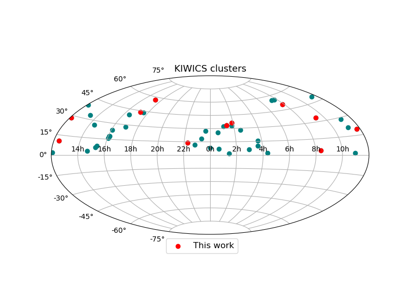
Figure 1: Sky Map of the full KIWICS sample. Red symbols correspond to the clusters analysed in this work.

Table 1: Main properties of the clusters . Column 1 corresponds to their names, columns 2 and 3 shows their coordinates, column 4 their redshift and columns 5,6 and 7 to their mass ($M_{500}$), radius (R₅₀₀) and luminosity (L₅₀₀) values (from the Piffaretti et al. 2011 catalogue).

Cluster name	RA (J2000)	DEC (J2000)	z	$M_{500}$	R500	L500a
	(hh:mm:ss)	(o:’:”)		$\times 10^{14}M_{\odot}$	Mpc	$\times 10^{44}$ erg s-1
RXJ0123.2+3327	01:23:12.2	33:27:40	0.0146	0.36	0.50	0.06
A262	01:52:45.0	36:09:25	0.0163	1.19	0.74	0.42
RXJ0123.6+3315	01:23:41.0	33:15:40	0.0164	0.61	0.60	0.14
A1367	11:44:36.5	19:45:32	0.0214	2.14	0.90	1.10
RXCJ0751.3+5012	07:51:22.5	50:12:45	0.0228	0.42	0.52	0.07
RXCJ0919.8+3345	09:19:49.2	33:45:37	0.0230	0.26	0.45	0.08
RXCJ2214.8+1350	22:14:52.7	13:50:48	0.0253	0.32	0.48	0.05
RXCJ1223.1+1037	12:23:6.50	10:37:26	0.0258	0.56	0.58	0.12
RXCJ1714.3+4341	17:14:18.6	43:41:23	0.0276	0.31	0.48	0.05
RXCJ1715.3+5724	17:15:21.9	57:24:27	0.0276	0.87	0.67	0.25
RXCJ1206.6+2811	12:06:37.4	28:11:01	0.0283	0.42	0.52	0.08
ZwCL1665	08:23:11.5	04:21:22	0.0293	0.73	0.63	0.19

• On average the uncertainties on the L₅₀₀ measurements range from 15 to 20 per cent (Piffaretti et al., 2011).

2.1 Data reduction

The reduction of the images was done with Astro-WISE (McFarland et al., 2013) following the same procedure as explained in detail in Venhola et al. (2018) and in Mancera Piña et al. (2019). Here, we briefly summarise the main steps.

The first phase of the data reduction consisted on the standard instrumental corrections; overscan, bias, and flat-fielding corrections were applied in all the sciences frames. The second phase took care of the sky subtraction followed by the astrometry and photometric corrections. For this last part, standard star fields that were observed at every night of observation were used for the calibration. Finally, with the sciences images cleaned of bad pixels and cosmic rays, they were median stacked and coadded into a single mosaic by using Swarp (Bertin, 2010) and sampled to a pixel size of 0.2 arcsec.

2.2 Sample selection and cluster properties

In this work, we analysed the clusters from the KIWICS sample with redshifts lower than 0.029. The poor quality of the final coadded image and the bad seeing of the observations made that seven clusters from the original sample were excluded, and that twelve clusters from KIWICS sample were considered. The fourth and fifth columns of Table 2 show the mean seeing for the $r$ and $g$ bands for each cluster. The twelve clusters considered in this study have a mean seeing of $\sim$ 1.4 arcsec in both $g$ and $r$ filters.

It also worth to mention that our final sample contains four clusters analysed already in Mancera Piña et al. (2019) where they studied eight clusters from KIWICS searching for ultra-diffuse galaxies (UDGs). In the present study we will analyse the properties of the dwarf galaxies. We considered as dwarf galaxies those with $M_{r}>-19.0$ mag and giant galaxies those with $M_{r}<-19.0$ mag. This limit was used following the historical convention to classify dwarf galaxies as those with $M_{B}>-18.0$ mag (Binggeli et al., 1988) and assuming a colour $B-r\sim 1.0$ mag for these galaxies. We also considered a low luminosity cut at $M_{r}=-15.5$ mag. Galaxies fainter than this limit were not analysed to avoid strong contamination of background objects.

Radial velocities for the galaxies in our clusters were obtained from Sloan Digital Sky Survey (SDSS) , NASA/IPAC Extragalactic Database (NED), and data from WIYN telescope. This spectroscopic data was used to estimate the cluster membership, the mean velocity ($V_{c}$) and the velocity dispersion of each cluster ($\sigma_{c}$). Figure 2 shows the velocity histograms of the clusters and Table 2 lists the velocity dispersion of the clusters. Both, the cluster membership and the velocity dispersion of the clusters were obtained by using a sigma clipping algorithm. In particular, we used a 3-$\sigma$ clipping to determine the cluster membership and a 2-$\sigma$ clipping for the velocity dispersion. In Figure 2 it is highlighted a 3-$\sigma_{c}$ range around the cluster central redshift (dashed vertical grey lines), which is the range we considered for cluster members. Note that there are three clusters; RXCJ1714.3+4341, RXJ0123.2+3327 and RXJ0123.6+3315, the first one with very few objects with spectroscopic redshifts available, and the last two having a mixed redshift distribution as they are in the same field of view.

The measured $\sigma_{c}$ was used to compute the $R_{200}$ radius of the clusters following $R_{200}=\sqrt{3}\sigma_{v}/10H(z_{c})$ (Carlberg et al., 1997). In addition, the halo mass ($M_{200}$) was obtained following the velocity dispersion-mass relation from Munari et al. (2013). In general, the values of $\sigma_{c}$ are in a range $\sim$ 175 km/s to $\sim$ 580 km/s. The clusters Abell 1367, RXCJ1715.3+5724, and Abell 262 have the largest values of the velocity dispersion and are accordingly the most massive ones? (see Table 1). Figure 3 shows the $M_{200}$ mass we estimated for each clusters as a function of their $M_{500}$ mass from Piffaretti et al. 2011 (values from X-ray measurements). We also added the values of $M_{200}$ computed by Mancera Piña et al. (2019) for their KIWICS subsample. The uncertainties in $M_{200}$ were obtained by using Monte Carlo error propagation, while the uncertainty for $M_{500}$ is assumed to be fifteen percent of the mass. This last assumption was done based on the average measurement uncertainties for L₅₀₀ explained in Piffaretti et al. (2011), which range from 15 to 20 percent. Certainly, it is worth to mention that any under/sub estimation of the velocity dispersion may also affect the estimation for $M_{200}$ and $R_{200}$ (e.g., clusters RXJ0123.2+3327 and RXJ0123.6+3315).

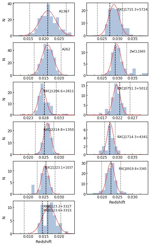
Figure 2: Redshift distributions for each cluster. The black dotted line marks the central redshift of the cluster, while the dotted grey lines indicate three times the velocity dispersion on each side. The fitted gaussian for the objects between the grey dotted lines is also shown in red colour. Note that the redshift distribution for clusters RXJ0123.2+3327 and RXJ0123.6+3315 are mixed (bottom panel) as they are in the same field of view.

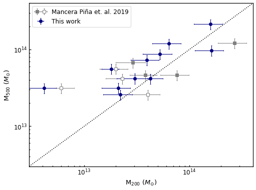
Figure 3: $M_{500}$ mass from Piffaretti et al. (2011) as a function of the $M_{200}$ mass we estimated from the velocity dispersion for each cluster. The filled and open grey points correspond to the clusters analysed in Mancera Piña et al. (2019), the open symbols corresponding to the four clusters that we have in common. The blue points correspond to the clusters analysed in this work.

Table 2: Properties of the clusters. Column 2 and 3 show the estimated values for the velocity dispersion and $M_{200}$. Columns 4 and 5 show the seeing of the coadd image in the $r$ and $g$ band. Last column shows the status classification we gave the cluster. The errors in the velocity dispersion values come from the Gaussian fit (Fig. 2).

Cluster	velocity dispersion	$M_{200}$	seeing $r$-band	seeing $g$-band	status
	(km/s)	$\times 10^{13}M_{\odot}$	(arsec)	(arsec)	(relaxed?)
RXJ0123.2+3327	483 $\pm$95	0.5 $\pm$ 0.2a	1.6	1.3	ub
A262	402 $\pm$24	5.0 $\pm$ 1.5	1.5	1.4	u
RXJ0123.6+3315	483 $\pm$95	0.5 $\pm$ 0.2a	1.6	1.3	ub
A1367	581 $\pm$64	15.0 $\pm$ 4.6	1.5	1.6	n
RXCJ0751.3+5012	360 $\pm$24	3.5 $\pm$ 1.1	1.3	1.3	n
RXCJ0919.8+3345	299 $\pm$19	2.0 $\pm$ 0.6	1.4	1.4	y
RXCJ2214.8+1350	351 $\pm$07	3.3 $\pm$ 1.0	1.3	1.3	u
RXCJ1223.1+1037	302 $\pm$12	2.1 $\pm$ 0.6	1.6	1.5	y
RXCJ1714.3+4341	176 $\pm$22	2.6 $\pm$ 0.8	1.3	1.5	y
RXCJ1715.3+5724	475 $\pm$29	8.1 $\pm$ 2.6	1.3	1.5	u
RXCJ1206.6+2811	381 $\pm$42	4.2 $\pm$ 1.3	1.5	1.4	n
ZwCL1665	382 $\pm$15	4.3 $\pm$ 1.3	1.3	1.4	u

• Same estimated mass for RXJ0123.2+3327 and RXJ0123.6+3315.

• Status unknown.

To complement the cluster properties we also looked at their dynamical status, whether it might be a relaxed system or not, to later see if there is any correlation with their dwarf properties. To identify reliably relaxed and unrelaxed clusters different approaches are commonly employed. The relaxation state is often inferred from the X-ray morphology (e.g. Mantz et al., 2015) and the distribution of relative velocities in clusters (e.g. Ribeiro et al., 2013). Here, we performed a visual check on the X-ray contour maps available in the literature (Kim & Fabbiano, 1995; Jones & Forman, 1999; Dahlem & Thiering, 2000; Russell et al., 2007; Eckmiller et al., 2011; Russell et al., 2014) and classified the clusters as relaxed when the X-ray contour have circular shape. We used the Shapiro test to check whether the galaxy velocity distribution of each cluster has a normal distribution (see the result in Table 3 and Fig. 2). We classified a cluster (last column on Table 2) as relaxed if it satisfies both tests, otherwise we just classified it as unknown status.

Table 3: Results of the Shapiro test to check the normality of the redshift distribution for the galaxies inside 3-$\sigma_{c}$ (Fig. 2). A p-value less than significance level (often 0.05) means we can reject null hypothesis that it is normally distributed.

Cluster name	p-value
RXJ0123.2+3327	0.17
A262	0.27
RXJ0123.6+3315	0.17
A1367	0.04
RXCJ0751.3+5012	0.05
RXCJ0919.8+3345	0.41
RXCJ2214.8+1350	0.22
RXCJ1223.1+1037	0.72
RXCJ1714.3+4341	0.94
RXCJ1715.3+5724	0.03
RXCJ1206.6+2811	0.01
ZwCL1665	0.62

3 SExtractor catalogues

The detection and the measurements of the photometric properties of the objects in the scientific images was done by using Source Extractor (SExtractor; Bertin & Arnouts, 1996) in dual mode: the $r$-band images of the clusters were used for the detection and the measurements of the photometric parameters of the objects in this band. The $g$-band parameters were measured at the position of the objects detected in the $r$-band image. In addition, SExtractor was run using two different configurations. In the first pass, the configuration used was similar to the one by Mancera Piña et al. (2019). This configuration is optimised to detect small and faint galaxies. In the second pass, we used a different configuration to detect large and bright galaxies (Appendix A). The final catalogues were a combination of the two SExtractor runs. For the common objects in both catalogues, their properties were taken from the faint catalogue.

The criteria to select galaxies from the full detection catalogues was made based on the SExtractor stellarity $\mathrm{CLASS\_STAR}$ and FLAG parameters. We consider as galaxies those objects with CLASS$\_$STAR $\leq$ 0.2 in both filters $g$ and $r$ and with $\mathrm{FLAGS_{r}=0}$, that ensure that we are not considering objects that are blended with any other close object or without accurate photometry.

The zeropoint calibration was applied to the MAG$\_$AUTO magnitude. It was obtained using the stars (objects with $\mathrm{CLASS\_STAR_{g,r}\geq 0.8}$ and $\mathrm{FLAGS_{r}=0}$) located in our fields and with magnitudes measured in SDSS. Only one cluster, A262, was not in the SDSS footprint. In this case, we used the Pan-STARRS survey (Chambers et al., 2016) to calibrate the photometry. The final calibration contains also the Galactic extinction correction. This was obtained by using the extinction calculator of NED (Schlafly & Finkbeiner, 2011). We did not apply k-correction to our magnitudes since its effect is not significant at the redshifts of our clusters (see for example Chilingarian et al. 2010).

3.1 Background decontamination

In order to remove background objects of the SExtractor catalogue, firstly we imposed a cut in colour $g-r$ $\leq$ 1.0 mag excluding all galaxies redder than this colour limit, which correspond to a 12 Gyr old stellar population with [Fe/H] = +0.25 supersolar metallicity (Worthey, 1994). The fraction of cluster members with $g-r>1.0$ mag is expected to be small according to the galaxy colour distribution in the nearby Universe (Hogg et al., 2004; Rines & Geller, 2008; Venhola et al., 2018). Figure 4 shows the colour-magnitude diagram (CMD) for the galaxies of all clusters of the sample in the whole field of view of the images and the cut in colour we imposed (dashed line in the top panel).

However, we might still have some contamination of foreground and background galaxies even applying a colour cut, as they can have a $g$ - $r$ $<$ 1.0 mag so we performed a second cut using the surface brightness-magnitude plane (similar to Venhola et al. 2018). To perform this selection, all the clusters of our sample were analysed together (bottom panel; Fig.4 ) in order to have a robust number of spectroscopically confirmed (and not confirmed) galaxy members. We fitted a linear relation of $M_{r}-\mu_{e}$ described by the galaxy cluster members (green points in Fig. 4). We considered as background objects those galaxies located more than 1.5-$\sigma$ (black dashed line in Fig. 4) above the linear relation in the $M_{r}-\mu_{e}$ defined by the cluster members.

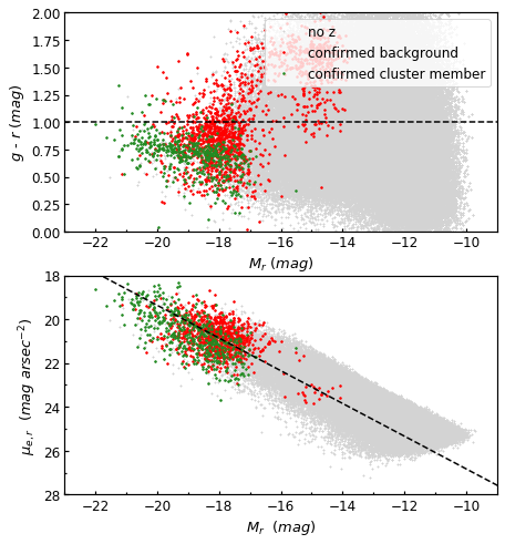
Figure 4: Top panel: colour-magnitude diagram for the galaxies of all the clusters grey symbols. The black dotted line highlights the colour $g-r$ $\leq$ 1.0 mag used to discard background galaxies. Bottom panel: Mean surface brightness of the galaxies that have passed the first colour cut as a function of their absolute magnitude (grey symbols). For a fixed absolute magnitude, we considered cluster members to be those galaxies below the black dotted line. See text for more details. In both panels, green and red points represent spectroscopically confirmed cluster members and background galaxies, respectively.

3.2 Visual classification

We also implemented a visual classification of the galaxies in our sample brighter than $m_{r}=20$ mag. Objects fainter than this magnitude are difficult to classify. The visual classification was also used to remove background galaxies that were not detected by using the colour and surface brightness cuts described previously. Following similar visual classifications in clusters (see Venhola et al., 2019; Wittmann et al., 2020), we visually classify the galaxies in five groups: late type, early type, background, interacting and unknown. Our classification is as follows,

• Early type galaxies: Galaxies with a uniform red colour (no blue patches) and morphology, not showing any clear spiral structure.

• Late type galaxies. In this category were included blue galaxies, showing structure features. In particular, the fainter objects that were included in this group were those that did not have a uniform colour, that is, with some characteristics such as blue spots.

• Likely background objects: Any object showing an irregular shape (with possible features like bars or spiral arms) was included in this category.

• Unknown. Any object that is an artefact or an star. Also objects that due to their faint magnitude are difficult to include in any category.

• Likely interacting objects. Any object that seems to be merging or interacting with another one.

The final sample excludes all the objects we classified as background, artefacts, interactions or unknown objects and, as mention, all objects with $m_{r}$ $>$ 20 mag, as the visual classifications there become not accurate. In Table 4 we provide an overview of the number of the final sample down to an absolute magnitude, M_r $\leq$-15.5 mag.

Table 4: Number of the final sample (dwarf plus giant galaxies) down to an absolute magnitude, M_r $\leq$ -15.5 mag.

Cluster	final sample
	(after visual classification)
A1367	542
RXCJ1715.3+5724	306
A262	468
ZwCL1665	290
RXCJ1206.6+2811	446
RXCJ0751.3+5012	166
RXCJ2214.8+1350	175
RXCJ1714.3+4341	304
RXCJ1223.1+1037	217
RXCJ0919.8+3345	343
RXJ0123.2+3327	248

3.2.1 Background contamination

In order to quantify how much contamination may still be present in the final sample, particularly in the dwarf regime (-19.0 mag $\leq$ M_r $\leq$ -15.5 mag) despite the visual classification we did, we estimated statistically the number of background galaxies we might expect from a blank field. The field used for this purpose was observed in the same way as in the clusters and we used the same criterion as in the clusters to select galaxies from its SExtractor catalogue, this is same colour and surface brightness cut. We selected a circular area of 0.38 deg² by using the image in the $r$-band, and estimated the number of dwarf galaxies present in the field and later we re-scaled this number to the area of each cluster. In Figure 5 we show the number of dwarfs expected to be background as a function of the number of dwarfs that we excluded in our visual classification. The figure shows that the number of dwarfs removed using visual classification agrees reasonably well with the one expected from the blank field.

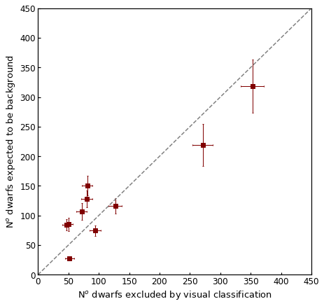
Figure 5: Number of dwarfs excluded by visual classification as function of the number of dwarfs expected to be background galaxies (from a blank field). Error bars correspond to Poisson uncertainties based on the actual number of objects.

4 Results

4.1 Distribution of dwarf and giant galaxies in clusters

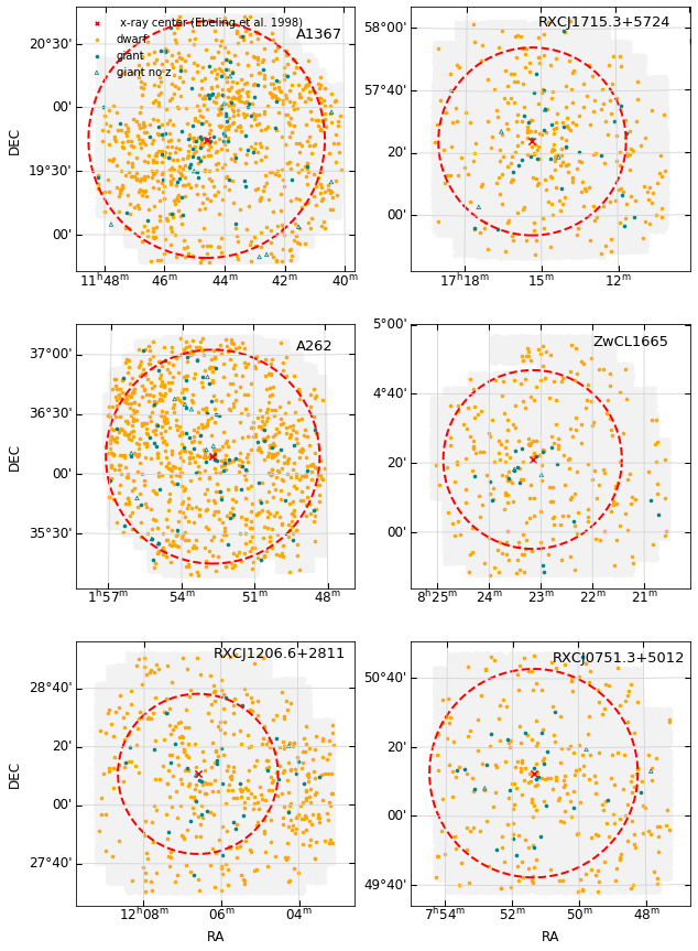
Figure 6: Distribution of dwarfs (yellow) and giants (teal) galaxies for each cluster. Teal circles correspond to giants for which redshift are available (mostly from SDSS) while teal open triangles correspond to giants without redshift available to confirm their cluster membership. A red marker highlights the X-ray centre from Ebeling et al. (1998), the red circle indicates the estimated $R_{200}$ radius, and the grey area indicates the field covered by the image in the $r$-band. (continued).

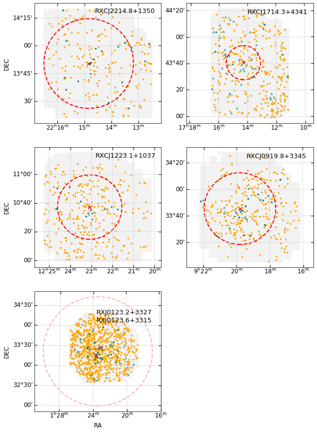
Figure 6 (Cont.): Distribution of dwarfs (yellow) and giants (teal) galaxies for each cluster. A red marker highlights the X-ray centre from Ebeling et al. (1998), the red circle indicates the estimated $R_{200}$ radius, and the grey area indicates the field covered by the image in the $r$-band. Note that in the last panel the two red markers correspond to two different X-ray defined clusters of our sample that are in the same field of view.

There are links between galaxy properties and their location in nearby galaxy clusters; for instance the morphological segregation observed in galaxy aggregations like Virgo (Lisker et al., 2007), Coma (Aguerri et al., 2004), Fornax (Venhola et al., 2019) or other nearby clusters (Sánchez-Janssen et al., 2008). This segregation is observed in a wide range of galaxy luminosities.

In Figure 6 and 6 (Cont.) we show the spatial distribution of the dwarf ($M_{r}$ $\geq$ -19.0 mag, orange points) and giant ($M_{r}$ $<$ -19.0 mag, green points) galaxies in the field of view of each cluster. Note that, all the clusters are covered at least until 1$R_{200}$, where it is also highlighted the X-ray centre (red cross symbol) for each cluster (Ebeling et al., 1998; Piffaretti et al., 2011).

A visual inspection of Figs. 6 and 6 (Cont.) shows that dwarf galaxies tend to be widely distributed across the clusters but not always homogeneously, as in some cases they tend to cluster in certain specific regions. For example, in A1367, which is the most massive and populated cluster in our sample, dwarfs tend to be localised in the central region but also in the substructures identified in this cluster the NE and SW regions (e.g. Ge et al., 2020). Giant galaxies in this cluster follow the same distribution. In the cluster RXCJ1715.3+5724 dwarfs tend to be more concentrated in the central region, a similar distribution is also seen in clusters ZwCL1665, RXCJ1206.6+2811, RXCJ1714.3+4341, RXCJ0751.3+5012, RXCJ1223.1+1037, RXCJ2214.8+1350, RXCJ1714.3+4341 and RXCJ0919.8+3345. A262 shows a wide distribution of their dwarf galaxies across the cluster but with some over densities in the border of the $R_{200}$ radius that might be due to the fact that this cluster is embedded in the Perseus supercluster so there is large substructure of galaxies around it. With respect to the clusters RXJ0123.2+3327 and RXJ0123.6+3315, since both are in the same field of view, their population of galaxies is mixed and because there are not enough redshift for the galaxies in those clusters, it is not easy to analyse their dwarf and giant distributions separately.

We used a Kolmogorov-Smirnov (KS) test to analyse the statistical differences between the giant and dwarf distributions within $R_{200}$. Figure 7 shows the cumulative distribution function of the clustercentric distance for both giant and dwarf distributions on each cluster. Table 5 contains the values of the probability given by the KS test. In particular, five clusters (A1367, RXCJ1715.3+5724 , A262, ZwCL1665 and RXCJ1223.1+1037) show dwarf and giant radial distributions which are statistically different. In these cases, the bright galaxies are located closer to the cluster centre. Moreover, these cases correspond to the more massive ones in our sample (as given by $M_{500}$ mass); other parameters such as velocity dispersion ($M_{200}$ indicator) or the dynamical status do not show any clear difference. The remaining five clusters (RXCJ1206.6+2811, RXCJ0751.3+5012, RXCJ2214.8+1350, RXCJ1714.3+4341, and RXCJ0919.8+3345) show a statistically similar radial distribution of dwarf and giant galaxies. The clusters RXJ0123.2+3327 and RXJ0123.2+3327 were not included in this figure (and in the following figures) as their field of view overlap and $R_{200}$ is not well determined.

Note that in some clusters (i.e. ZwCL1665, RXCJ1206.6+2811, RXCJ0751.3+5012, RXCJ2214.8+1350, RXCJ1714.3+4341, and RXCJ0919.8+3345) the distributions of the giants start at larger distances, not necessarily at the cluster centre. The reason for this is an small offset between the X-ray centre we are using (Ebeling et al., 1998; Ebeling et al., 2000, ;ROSAT observations) and the position of of the brightest cluster galaxy.

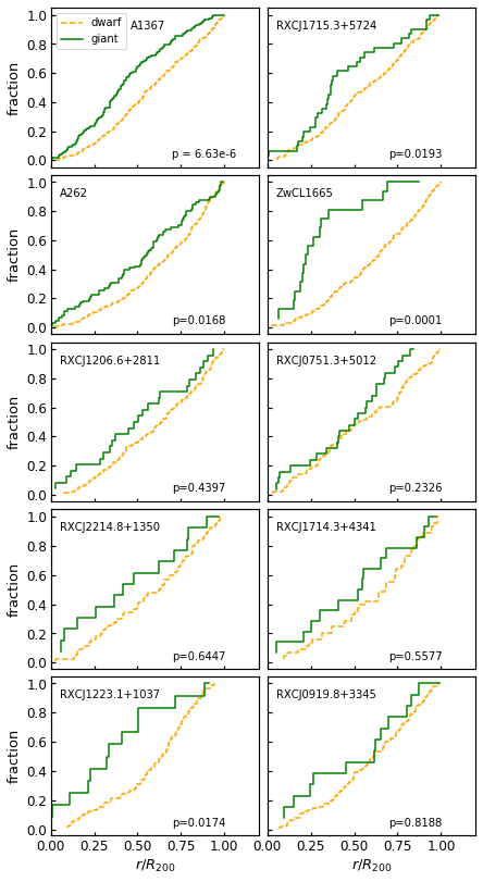
Figure 7: Individual cumulative functions of the clustercentric distances of dwarfs (yellow dashed line) and giants (green line) on each cluster. The number at the corner of each panel corresponds to the p-value coming from a Kolmogorov-Smirnov test which gives the probability that giants and dwarfs are taken from the same radial distribution.

4.2 The dwarf galaxy fraction

We quantified the dwarf galaxy fraction (defined as the ratio between the number of dwarfs over the total number of galaxies - dwarfs plus giants - within $R_{200}$) for each cluster as shown in Table 5 (column 1). The dwarf fraction ranges from $\sim$0.75. to $\sim$ 0.91 in all clusters, with small scatter at a fixed mass. Apparently, there is not relation between the dwarf fraction and the dynamical status, mass or velocity dispersion of the clusters (see Table 2). We discuss this further in Section 5.

Table 5: Dwarf fraction and blue dwarf fraction on each cluster. Column 2 corresponds to the dwarf fraction, while column 3 corresponds to the p-value resulting after applying a Kolmogorov-Smirnov test for clustercentric distance distributions between dwarf and giants (Fig. 7). Column 4 corresponds to the blue dwarf fraction (Fig. 12), while column 5 corresponds to the p-value after applying a KS test between the clustercentric distribution of blue and red dwarfs. Errors correspond to a binomial uncertainties.

Cluster	dwarf fraction	giant-dwarf galaxies	blue dwarf fraction	blue-red dwarfs
		(p-value)		(p-value)
A1367	0.75 $\pm$0.02	6.6e-6	0.29 $\pm$0.02	0.0063
RXCJ1715.3+5724	0.86 $\pm$0.02	0.0193	0.10 $\pm$0.02	0.0761
A262	0.82 $\pm$0.02	0.0168	0.21 $\pm$0.02	0.3974
ZwCL1665	0.91 $\pm$0.02	0.0001	0.31 $\pm$0.04	0.0542
RXCJ1206.6+2811	0.88 $\pm$0.02	0.6584	0.17 $\pm$0.03	0.1811
RXCJ0751.3+5012	0.79 $\pm$0.04	0.7223	0.24 $\pm$0.04	0.8750
RXCJ2214.8+1350	0.87 $\pm$0.03	0.6447	0.18 $\pm$0.04	0.1208
RXCJ1714.3+4341	0.76 $\pm$0.06	0.5777	0.16 $\pm$0.05	0.8012
RXCJ1223.1+1037	0.89 $\pm$0.03	0.0174	0.16 $\pm$0.04	0.4329
RXCJ0919.8+3345	0.85 $\pm$0.03	0.8188	0.31 $\pm$0.04	0.0003

4.3 Structural parameters for dwarf and giants

The dependence of the distribution structural parameters on the environment has been studied in some nearby galaxies clusters, such as the Coma cluster (see Trujillo & Aguerri, 2004; Venhola et al., 2019; Janz et al., 2014). We used GALFIT (Peng et al., 2010) to determine the structural parameters of the galaxies in our clusters. In particular, we run GALFIT as is described in Venhola et al. (2018) for all the possible cluster members but excluding all the objects with the SExtractor parameter ISORAREA-IMAGE being smaller than 200 pixels. This cut was mainly done to exclude smaller objects that are likely to have a bad fit as they are very faint (apparent $r$-band magnitudes fainter than $\sim 22$ mag). All the objects were fitted using a single Sérsic function in both $r$ and $g$ bands. Given the resolution of our images we were not able to distinguish a nucleus in the galaxies. We inspected the best fits by checking the output parameters, and considered as bad fits those with effective radius close to zero, also were excluded those objects with a significant (more than 0.5 mag) difference between SExtractor and GALFIT magnitudes.

Figure 8 shows the Sérsic index ($n$) of the dwarf galaxies as a function of the clustercentric distance. We divided the dwarf sample according to the visual classification (described in Section 3.2), in early (dE) and late type dwarfs (dIrr). In six (A1367, RXCJ1715.3+5724, A262, ZwCL1665, RXCJ1206.6+2811, RXCJ1223.1+1037) out of the ten clusters there seems to be a trend in the values of the Sérsic index for the dE galaxies. In particular, the values of $n$ increase towards the inner regions of the clusters as shown in Table 6, which lists the mean value of $n$ computed in the inner ($r$ $\leq$ 0.3$R_{200}$) and the outer cluster regions (0.3$R_{200}$ $<$ $r$ $\leq$ $1R_{200}$). This indicates that dwarfs located in the inner cluster regions have more concentrated light profiles than those located in the outer regions. This result can be explained if galaxies in the inner cluster regions are more affected by environmental effects than those located in the outskirts of the clusters (e.g. Trujillo et al., 2002). It is also possible that more concentrated dwarfs have survived the cluster environment of the inner regions while those with a flatter profile have not. The trend observed for the values of $n$ in the dE sample is not present for the late-type dwarf galaxies.

Table 6: Mean value for the Sérsic index $n$ (columns 2 and 3) and the effective radius (columns 4 and 5) measured in bins of clustercentric distance, $r/R_{200}\leq$0.3 and 0.3$<r/R_{200}\leq$1.0. The error value corresponds to the standard deviation measured in each distance bin normalised by the square root of the total value on each bin. Note that these values are for those dwarfs classified as dwarf ellipticals.

Cluster	mean $n$	mean $n$	mean $R_{\rm eff}$ (kpc)	mean $R_{\rm eff}$ (kpc)
	$r/R_{200}\leq$0.3	0.3$<r/R_{200}\leq$1.0	$r/R_{200}\leq$0.3	0.3$<r/R_{200}\leq$1.0
A1367	1.52 $\pm$ 0.09	1.21 $\pm$ 0.04	1.32$\pm$ 0.07	1.30$\pm$ 0.03
RXCJ1715.3+5724	1.38 $\pm$ 0.11	1.09$\pm$ 0.04	1.49$\pm$ 0.08	1.32$\pm$ 0.05
A262	1.54$\pm$ 0.09	1.26$\pm$ 0.05	1.23$\pm$ 0.09	0.90$\pm$ 0.03
ZwCL1665	1.50$\pm$ 0.08	1.14$\pm$ 0.08	1.38$\pm$ 0.10	1.24$\pm$ 0.04
RXCJ1206.6+2811	1.53$\pm$ 0.12	1.08$\pm$ 0.06	1.26$\pm$ 0.07	1.26$\pm$ 0.04
RXCJ0751.3+5012	1.46$\pm$ 0.15	1.29$\pm$ 0.09	1.42$\pm$ 0.10	1.20$\pm$ 0.07
RXCJ2214.8+1350	1.38$\pm$ 0.09	1.12$\pm$ 0.08	1.27$\pm$ 0.08	1.28$\pm$ 0.07
RXCJ1714.3+4341	1.56$\pm$ 0.15	1.32$\pm$ 0.07	1.46$\pm$ 0.12	1.32$\pm$ 0.06
RXCJ1223.1+1037	1.56 $\pm$ 0.19	1.36$\pm$ 0.27	1.39$\pm$ 0.16	1.30$\pm$ 0.16
RXCJ0919.8+3345	1.27$\pm$ 0.13	1.30$\pm$ 0.07	1.29$\pm$ 0.09	1.37$\pm$ 0.07

In addition to the Sérsic index, in Figure 9 we also show the effective radius ($R_{\rm eff}$) as a function of the clustercentric distance, and similarly we quantify the mean value of $R_{\rm eff}$ in the inner and the in outermost region of the clusters (see Table 6). Although most of the clusters show a slightly higher mean value of $R_{\rm eff}$ in the inner regions, these differences are smaller than 2-$\sigma$.

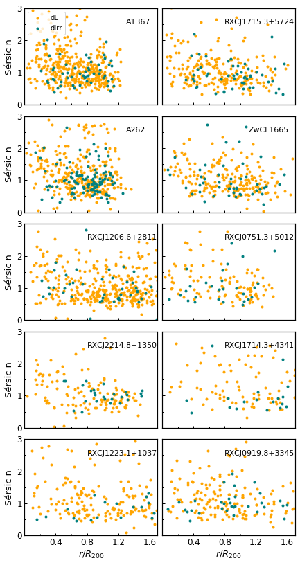
Figure 8: Sérsic index ($n$) as a function of clustercentric distance for early type dwarfs (orange points) and late type dwarfs (green points). Note that cluster RXJ0123.2+3327 and RXJ0123.2+3315 are not included in this figure.

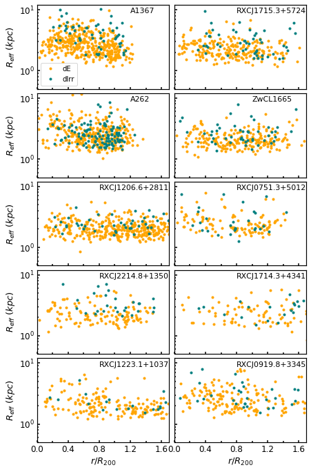
Figure 9: Effective radius ($R_{\rm eff}$) as a function of clustercentric distance for early type dwarfs (orange points) and late type dwarfs (green points). Note that cluster RXJ0123.2+3327 and RXJ0123.2+3315 are not included in this figure.

4.4 The $g-r$ colour of galaxies

We classified the galaxies in blue and red according to their $g-r$ stellar colour. This classification was done according to their position in the CMD. Figure 10 shows the CMD of the galaxies in all clusters. The green points represent those galaxies confirmed spectroscopically as cluster members. Using an iterative sigma-clipping algorithm, we fitted the red sequence of this global CMD that was used to split between blue and red galaxies. We considered as blue galaxies those with a $g-r$ colour bluer than 3-$\sigma$ (bottom line), being $\sigma$ the dispersion in colour of the galaxies around the red sequence.

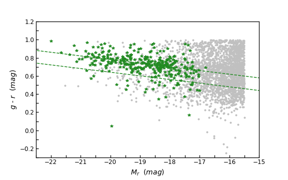
Figure 10: Colour-magnitude diagram for all the red sequence elliptical galaxies (green points) of all cluster of the sample espectrally confirmed as a cluster member. Upper green line corresponds to the fit line for these galaxies while the bottom green line is the same line shifted three sigmas (standard deviation of the distance of the the green points to the fitting line) below. Grey points correspond to the remaining galaxies from each cluster.

Figure 11 shows the colour-magnitude diagrams of the individual clusters inside 1$R_{200}$ and up to the absolute magnitude, M_r = -15.5 mag (dashed line on each panel). We overplotted in this figure the red sequence fitted in the global CMD and the line used for the blue and red galaxy separation. Overall, the global red sequence line traces well the red sequence of each individual cluster. Note that the few bright galaxies without available redshifts are also included in this figure. Interestingly, the number of blue galaxies varies from cluster to cluster, with some of clusters having very few blue galaxies, especially large blue galaxies (for example clusters RXCJ1223.1+1037, RXCJ0751.3+5012, and RXCJ2214.8+1350) while there are others where the blue galaxy population is larger (see A1367).

Figure 12 shows the cumulative distribution functions of the blue and red galaxies plotted as a function of their clustercentric distance. We quantified the differences between the blue and red dwarf distributions (filled lines) by using the KS test (p-values in Table 5). According to this test, three clusters (A1367, ZWCL1665 and RXCJ0919+3345) show blue and red dwarf distributions that are statistically different; in those cases, red dwarfs are located closer to the cluster centre. We find no correlation with clusters mass, velocity dispersion or dynamical status (see Table 2). In contrast, the remaining eight clusters show a similar radial distribution for blue and red dwarfs.

When checking the cumulative fraction for giant galaxies (dashed lines in Figure 12), we see that overall red giants tend to be distributed closer to the cluster centre than blue giant galaxies. Note that in some clusters, like RXCJ1206.6+2811 and RXCJ2214.8+1350 there are no blue giant galaxies inside $R_{200}$ so all the bright galaxies in those clusters are red (see also Figure 11).

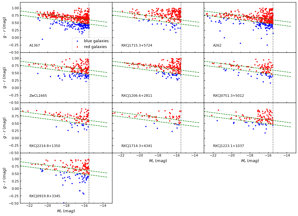
Figure 11: Colour-magnitude diagram for each cluster. Blue point highlights the "blue" galaxies while the red points highlights the "red" galaxies. Green dashed lines indicate the lines we traced for the red sequence and to do the selection between blue and red galaxies (see Figure 10). Black dotted line marks an absolute magnitude, M_r $=$ -15.5 mag, limit that we used in all the clusters.

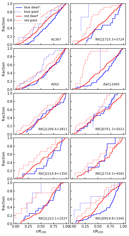
Figure 12: Individual cumulative fractions as a function of the distance to the cluster centre for the blue and red galaxies. Blue and red dashed lines correspond to the ’blue’ dwarfs and ’red’ dwarf respectively, while blue and red filled lines lines correspond to ’blue’ giants and ’red’ giants respectively.

5 discussion

5.1 Environmental effects

In the previous sections we studied the spatial distribution of dwarf galaxies, their colours, Sérsic indices, and effective radii for each cluster. In the following, we discuss how these properties change depending on the environment; whether there are differences in the properties of the dwarfs that depend on the mass, velocity dispersion or dynamical status of the cluster.

5.1.1 Distribution of dwarfs vs. giants

In Section 4.1 we showed the distribution of the dwarf candidates in the different clusters of the sample and saw that they dominate in number the galaxy population of the clusters. When comparing the clustercentric distribution of giants and dwarfs, we find that the distribution of giants and dwarfs is different in five of the clusters. In these cases, the bright galaxies are located closer to the cluster centre. In particular, these cases correspond to the more massive clusters of the sample, as given by $M_{500}$ mass (values that come from X-ray flux measurements, see Fig. 7 and Table 2). When using the velocity dispersion as a mass ($M_{200}$) indicator the correlation is less clear. We quantified the ratio between the fraction of dwarfs inside 0.3$R_{200}$ and the fraction between 0.3$R_{200}$ and 1$R_{200}$ (see the second row in Fig. 13). We found that in all cases this ratio is lower than 1, meaning that the fraction of dwarfs is lower at short distances from the cluster centre, in agreement with earlier results in the literature (e.g. Popesso et al., 2005; Rude et al., 2020). A similar finding was noted in Mancera Piña et al. (2018) where a lack of UDGs is reported near the cluster centres.

The lack of dwarfs in the cluster core can be explained by several effects. One is tidal disruption of the dwarfs in the very inner regions (see Popesso et al., 2005). Another possibility is that giants suffer stronger dynamical friction, making them spiral inward to the cluster centre. While this mass segregation has been studied theoretically (Kim et al., 2020) and observationally (Roberts et al., 2015), there is still no consensus about the findings, as some studies find significant segregation while others find weak segregation in galaxy groups and clusters. We defer a more detailed analysis of the distribution of dwarfs and giants to a follow-up study.

5.1.2 The dwarf fraction in clusters

We find that the dwarf fraction defined as the ratio between the number of dwarfs over the total number of galaxies (dwarfs plus giants) within $R_{200}$, in all the clusters of our sample is larger than $\sim$ 0.7. In order to compare these dwarf fractions with well-studied, nearby clusters, such as Fornax (catalogue from Venhola et al. (2018), $\sigma_{c}$ $\sim$374 km/s (Drinkwater et al., 2001)) and Virgo (extended Virgo catalogue from Kim et al. (2014), $\sigma_{c}$ $\sim$800 km/s) we estimated the fraction of dwarfs in these clusters by selecting their galaxies in the same way as we did for our clusters (down to an absolute magnitude of M_r $\leq$-15.5 mag) as is shown in Fig. 13 (right panels). When comparing to Fornax, whose velocity dispersion falls into the regime of most of our clusters, we find that its fraction is smaller than in the clusters (regardless of the region where this fraction is measured) of our sample with as similar mass. It may be that there is still contamination by background galaxies present in our sample that could affect the dwarf fraction (Section 3.2.1) as most of the bright dwarfs in the Fornax sample are likely confirmed cluster members (Venhola et al., 2018). Additionally, there seems to be no relation between the dwarf fraction and the dynamical status of the clusters. Also, there is no clear relation with the distribution of dwarfs and giants (different colours in Fig.13).

As regards to Virgo, that cluster also has a relatively low fraction of dwarfs, however given its high velocity dispersion or mass (M = 1.2 $\times$ $10^{15}$ M_⊙, Fouqué et al. 2001), a comparison with the clusters of our sample, which are less massive, is not simple.

We do not measure a clear decrease in the dwarf fraction as a function of cluster mass, as seen in Popesso et al. (2005), who analysed 69 clusters in the $z$-band. Measuring the dwarf-to-giant ratio within a radius of 1 Mpc they found an anti-correlation with the cluster mass, velocity dispersion, and X-ray luminosity, however, the anti-correlation they found is less clear when the dwarf fraction is measured withing $R_{200}$ so in agreement with our result here. Although, their definition for dwarfs is different.

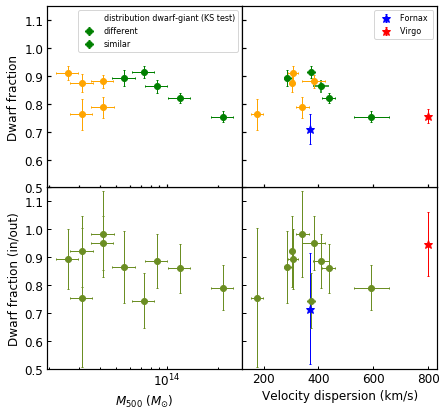
Figure 13: Top panels: Dwarf fraction inside $R_{200}$ as a function of cluster mass $M_{500}$ (left) and cluster velocity dispersion (right). Green colour points indicate whether the distribution of dwarfs and giants is different (based on the KS-test), while orange indicates that both distribution are similar. Bottom panels:Ratio of the dwarf fraction in the inner region and in the outermost regions of the cluster versus the same quantities.

5.1.3 Sérsic indices and Effective Radii across the clusters

We find hints that dwarfs are more concentrated (higher Sérsic index) in the central regions of the clusters (Fig. 14) and have larger effective radii (Fig. 15). In Venhola et al. (2019), the brighter dwarfs of the Fornax cluster (M_r $<$ -16.5 mag) tend to be more concentrated at shorter distances from the cluster centre (i.e. have large Sérsic indices), and they are also found to be smaller at those distances. The argument given in that work is in agreement with tidal interactions and a slow quenching in the inner region of a galaxy, possibly combined with extra central star formation making these galaxies more concentrated. Note that for fainter dwarfs their relation is opposite: such galaxies are larger in the inner parts of the cluster, with similar Sérsic indices. Janz et al. (2016) state that dwarfs located in the high-density environment of the Virgo cluster tend to be smaller, a picture that is in agreement with the Fornax dwarf sample. Our results for the Sérsic indices are compatible with nearby clusters, but for $R_{\rm eff}$ the situation is more complicated. Since the effects are likely to be strongly dependent on the mass of the dwarf, a detailed comparison is needed. We postpone this is to our next paper (Choque Challapa et al. in prep.).

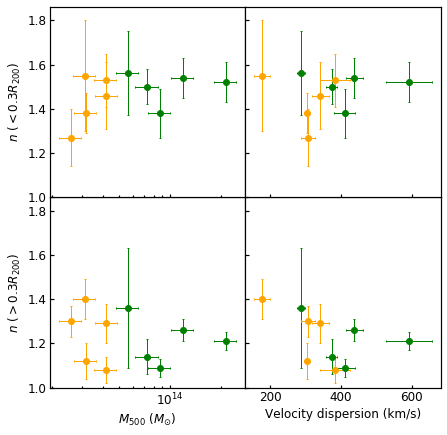
Figure 17: Sérsic index for dwarf ellipticals as a function of velocity dispersion and cluster mass, $M_{500}$ in the inner (top panels) and outer (bottom panels) region of each cluster. Green colour points indicate whether the dwarf and giant distributions are statistically different (based on the KS test), while orange indicates both distribution are statistically similar.

In addition, when comparing the average value of the Sérsic index in the inner and outer region of the clusters as is shown in Fig. 14, there seems to be a difference between the least massive and most massive clusters. This is, the average $n$ value is larger in the inner region (by about 0.3) for almost the full range of cluster mass or velocity dispersion (see also Appendix; top panels in Fig. 17) and decreases at further distances from the cluster core (bottom panels in Fig. 17); it tends to be a bit larger for the more massive clusters. Tidal interaction and/or ram-pressure stripping might explain why dwarfs become more concentrated at the cluster core and it seems to be that these effects are stronger in the more massive clusters. With regards to the difference in spatial distribution between the dwarf and giants galaxies in the cluster, we do not find any clear correlation as a function of the Sérsic index difference (different colours in Fig. 14). In a similar way, we do not find a correlation between the ratio of mean Sérsic indices and the dynamical status. Regarding the effective radius, when comparing its average value in the inner and outer regions, there is a weak tendency for this difference to be larger for more massive clusters.

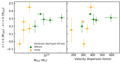
Figure 14: Difference between the mean Sérsic index value in the inner regions of the cluster ($r\leq$0.3$R_{200}$) and the mean value in the outer regions (0.3$R_{200}$ $<$ $r$ $\leq$1$R_{200}$) for the dwarf ellipticals as a function of cluster mass $M_{500}$ (left) and cluster velocity dispersion (right). Green colour points indicate whether the distribution of dwarfs and giants is different (based on the KS-test), while orange indicates that both distribution are similar.

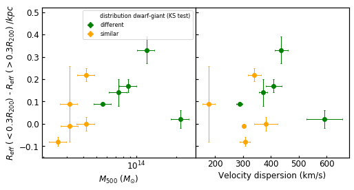
Figure 15: Difference between the mean value of effective radius in the inner regions of the cluster ($r\leq$0.3$R_{200}$) and the mean value in the outer regions (0.3$R_{200}$ $<$ $r$ $\leq$1$R_{200}$) for the dwarf ellipticals as a function of cluster mass $M_{500}$ (left) and cluster velocity dispersion (right). Same symbols and colours as in Figure 14.

5.1.4 Colours of galaxies

In the same way that most galaxies in clusters are dwarfs, most of them are red. Additionally, three clusters of our sample (A1367, ZwCl1665, RXCJ0919+3345) show blue and red dwarf spatial distributions that are statistically different (by taking a KS test, Table 5 and Fig. 12). In those cases, red, quiescent dwarfs, are located closer to the cluster centre, as has been previously reported on other clusters (e.g. Popesso et al., 2005). We checked whether these three clusters have common properties, such as cluster mass, velocity dispersion or dynamical status, but this is not the case (see Table 2). In contrast, the remaining eight clusters show radial distributions that are statistically similar for blue and red dwarfs. For completeness, we also checked the distribution for giant galaxies (Fig. 11, 12), and in some clusters like RXCJ1206.6+2811 and RXCJ2214.8+1350 there are no blue giant galaxies inside $R_{200}$.

When we look for a trend on the the blue dwarf fraction as a function of the cluster mass and velocity dispersion (top panels in Fig. 16), we find no correlation between these parameters, but we find that the blue dwarf fraction in all the clusters is less than 0.5. Moreover, when we compare with the Fornax and Virgo clusters, the blue dwarf fraction for Fornax is a bit smaller than in most clusters of our sample, while Virgo has a higher fraction, similar to three of our clusters. Also, the clusters with the highest fraction of blue dwarfs are those where the blue dwarfs are distributed differently than red galaxies, such that red dwarfs are generally situated closer to the cluster centre than blue ones. This agrees with the fact that the ratio of the blue dwarf fraction in the inner and the outer regions of the clusters is in most cases less than 1, indicating that the blue dwarf fraction increases when going away from the centre (see ratio bottom panels in Fig. 16). We find that these three cases with the highest blue dwarf fraction are not special, as far as their dynamical cluster status is concerned. A possible explanation for these three cluster is that we are seeing the cluster together with end-on filaments in front or behind, producing a line-of-sight contamination with blue dwarfs, which we expect to be more prevalent in filaments.

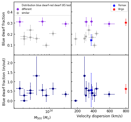
Figure 16: Top panels: Blue dwarf fraction inside $R_{200}$ as a function of cluster mass $M_{500}$ (left) and cluster velocity dispersion (right). Purple colour points indicate clusters for which the distribution of blue and red dwarfs is different (based on a KS test), while grey indicates that both distribution are similar. Bottom panels: Ratio of the blue dwarf fraction in the inner and outer regions of the cluster as a function of cluster mass $M_{500}$ (left) and cluster velocity dispersion (right).

6 Summary and Conclusion

In this work, we analysed a set of twelve nearby clusters from the KIWICS survey, studying the properties of the dwarf population in each cluster for galaxies as faint as a total $r$-band absolute magnitude, M_r $=$ -15.5 mag. We investigated their distribution in the cluster and their relative fraction, as compared to giant galaxies, and also determined their Sérsic index $n$ and their effective radius, $R_{\rm eff}$. Additionally, we studied the colour distribution of dwarfs to study differences between clusters and correlating them with their physical parameters, to better understand how the environment might affect the dwarf population. Our main results are summarised below,

• The dwarf galaxy population dominates by number in all the clusters but their distribution in each cluster is different: they tend to be distributed across the cluster but not always homogeneously. Regarding their distribution compared with giant galaxies, in half of the clusters of our sample, dwarfs are distributed in a statistically different way across the clusters than giants, with giants being closer to the cluster centre. These cases correspond to the more massive clusters of the sample. We find that the dwarf fraction in each cluster it is greater that $\sim$ 0.75 (Table 5), with small scatter at a fixed mass. Furthermore, when we compare the dwarf fraction in the inner and outer region of the cluster, we find that the dwarf fraction is larger in the outer regions (Fig. 13).

• We find that the average Sérsic index for those dwarfs we classified as early type or quiescent tends to increase at shorter distance from the cluster centre (Table 6). This trend is found in all the clusters regardless of their mass. We do not find similar trends for $R_{\rm eff}$.

• When exploring the colour distributions, we find that although red dwarf galaxies dominate in all the clusters of our sample, with the total blue fraction always less than $\sim$0.4 (Table 5), the fraction of blue dwarfs is about 50% lower in the central regions than in the outer parts of the cluster (Fig. 16).

To further understand the properties of dwarf galaxies in the different environments one limiting factor has been the absence of redshifts for the fainter dwarfs, to be able to determine their cluster membership. Although SDSS is providing many redshifts, better and deeper surveys are needed to provide enough objects to study properties like substructure in the dwarf population, which can tell us about how the cluster environment is influencing the formation and evolution of dwarf galaxies. This issue might be improved in the near future when the WEAVE nearby spectroscopic cluster survey, that includes all the clusters of our photometric survey, will provide us with thousands of new redshifts per cluster. In this way, our background contamination will drop and our analysis will be more accurate. While WEAVE will obtain intermediate resolution spectra in its MOS mode for all dwarf galaxies in the central regions down to a magnitude M${}_{r}<$-15 mag, the mIFU mode will allow us to obtain 2-dimensional internal properties of a selected subsample of dwarfs, giving us further information about the kinematic, mass distribution, stellar populations and metallicities for the dwarf population in these nearby clusters (e.g. Scott et al., 2020), which can then be compared with the properties of the clusters.

Data Availability

The data underlying this article will be shared upon a request to the corresponding authors. The raw data is stored in the Isaac Newton Group Archive.

Appendix A SExtractor configuration

Main SExtractor configuration parameters used for the smaller object detection.

DETECT MINAREA = 20, DETECT THRESHOLD = 2, ANALYSIS THRESHOLD = 2, BACK SIZE = 64.

For very large objects not detected with the above parameters,

DETECT MINAREA = 10000, DETECT THRESHOLD = 50, ANALYSIS THRESHOLD = 50, BACK SIZE = 21000.

Appendix B Sérsic indices and Effective Radii

In this appendix, we report the plots showing the average value of the Sérsic index and effective radius inside a distance of 0.3$R_{200}$ and outside (0.3$R_{200}$ $<$ $r$ $<$ 1$R_{200}$) for the different clusters as a function of their mass ($M_{500}$) and velocity dispersion.

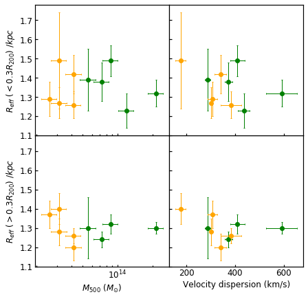
Figure 18: Effective radius for dwarf ellipticals as a function of velocity dispersion and cluster mass, $M_{500}$ in the inner (top panels) and outer (bottom panels) region of each cluster. Green colour points indicates whether the dwarf and giant distributions are statistically different (based on the KS test), while orange indicates both distribution are statistically similar.

References

- Aguerri et al. (2004) Aguerri J. A. L., Iglesias-Paramo J., Vilchez J. M., Muñoz-Tuñón C., 2004, AJ, 127, 1344
- Aguerri et al. (2005) Aguerri J. A. L., Iglesias-Páramo J., Vílchez J. M., Muñoz-Tuñón C., Sánchez-Janssen R., 2005, AJ, 130, 475
- Aguerri et al. (2018) Aguerri J. A. L., Agulli I., Méndez-Abreu J., 2018, MNRAS, 477, 1921
- Aguerri et al. (2020) Aguerri J. A. L., Girardi M., Agulli I., Negri A., Dalla Vecchia C., Domínguez Palmero L., 2020, MNRAS, 494, 1681
- Agulli et al. (2014) Agulli I., Aguerri J. A. L., Sanchez-Janssen R., Barrena R., Diaferio A., Serra A. L., Mendez-Abreu J., 2014, MNRAS, 444, L34
- Barkhouse et al. (2009) Barkhouse W. A., Yee H. K. C., López-Cruz O., 2009, ApJ, 703, 2024
- Bertin (2010) Bertin E., 2010, SWarp: Resampling and Co-adding FITS Images Together (ascl:1010.068)
- Bertin & Arnouts (1996) Bertin E., Arnouts S., 1996, A&AS, 117, 393
- Binggeli et al. (1988) Binggeli B., Sandage A., Tammann G. A., 1988, ARA&A, 26, 509
- Boselli & Gavazzi (2006) Boselli A., Gavazzi G., 2006, PASP, 118, 517
- Boselli et al. (2008) Boselli A., Boissier S., Cortese L., Gavazzi G., 2008, ApJ, 674, 742
- Boselli et al. (2011) Boselli A., et al., 2011, A&A, 528, A107
- Butcher & Oemler (1978) Butcher H., Oemler A. J., 1978, ApJ, 219, 18
- Carlberg et al. (1997) Carlberg R. G., Yee H. K. C., Ellingson E., 1997, ApJ, 478, 462
- Chambers et al. (2016) Chambers K. C., et al., 2016, arXiv e-prints, p. arXiv:1612.05560
- Chilingarian et al. (2010) Chilingarian I. V., Melchior A.-L., Zolotukhin I. Y., 2010, MNRAS, 405, 1409
- Cortese et al. (2021) Cortese L., Catinella B., Smith R., 2021, arXiv e-prints, p. arXiv:2104.02193
- Dahlem & Thiering (2000) Dahlem M., Thiering I., 2000, PASP, 112, 148
- Dalton (2016) Dalton G., 2016, in Skillen I., Balcells M., Trager S., eds, Astronomical Society of the Pacific Conference Series Vol. 507, Multi-Object Spectroscopy in the Next Decade: Big Questions, Large Surveys, and Wide Fields. p. 97
- Dressler (1980) Dressler A., 1980, ApJ, 236, 351
- Drinkwater et al. (2001) Drinkwater M. J., Gregg M. D., Colless M., 2001, ApJ, 548, L139
- Ebeling et al. (1998) Ebeling H., Edge A. C., Bohringer H., Allen S. W., Crawford C. S., Fabian A. C., Voges W., Huchra J. P., 1998, MNRAS, 301, 881
- Ebeling et al. (2000) Ebeling H., Edge A. C., Allen S. W., Crawford C. S., Fabian A. C., Huchra J. P., 2000, MNRAS, 318, 333
- Eckmiller et al. (2011) Eckmiller H. J., Hudson D. S., Reiprich T. H., 2011, A&A, 535, A105
- Fouqué et al. (2001) Fouqué P., Solanes J. M., Sanchis T., Balkowski C., 2001, A&A, 375, 770
- Fujita (2004) Fujita Y., 2004, PASJ, 56, 29
- Gavazzi et al. (2013) Gavazzi G., Fumagalli M., Fossati M., Galardo V., Grossetti F., Boselli A., Giovanelli R., Haynes M. P., 2013, A&A, 553, A89
- Ge et al. (2020) Ge C., et al., 2020, in American Astronomical Society Meeting Abstracts #235. p. 459.04
- Gnedin (2003) Gnedin O. Y., 2003, ApJ, 589, 752
- Hamraz et al. (2019) Hamraz E., Peletier R. F., Khosroshahi H. G., Valentijn E. A., den Brok M., Venhola A., 2019, A&A, 625, A94
- Hogg et al. (2004) Hogg D. W., et al., 2004, ApJ, 601, L29
- Janz et al. (2014) Janz J., et al., 2014, ApJ, 786, 105
- Janz et al. (2016) Janz J., Laurikainen E., Laine J., Salo H., Lisker T., 2016, MNRAS, 461, L82
- Janz et al. (2021) Janz J., Salo H., Su A. H., Venhola A., 2021, A&A, 647, A80
- Johnson et al. (2015) Johnson M. C., et al., 2015, MNRAS, 451, 3192
- Jones & Forman (1999) Jones C., Forman W., 1999, ApJ, 511, 65
- Kawata & Mulchaey (2008) Kawata D., Mulchaey J. S., 2008, ApJ, 672, L103
- Kenney et al. (2014) Kenney J. D. P., Geha M., Jáchym P., Crowl H. H., Dague W., Chung A., van Gorkom J., Vollmer B., 2014, ApJ, 780, 119
- Kim & Fabbiano (1995) Kim D.-W., Fabbiano G., 1995, ApJ, 441, 182
- Kim et al. (2014) Kim S., et al., 2014, ApJS, 215, 22
- Kim et al. (2020) Kim S., Contini E., Choi H., Han S., Lee J., Oh S., Kang X., Yi S. K., 2020, ApJ, 905, 12
- Koch et al. (2012) Koch A., Burkert A., Rich R. M., Collins M. L. M., Black C. S., Hilker M., Benson A. J., 2012, ApJ, 755, L13
- Koleva et al. (2013) Koleva M., Bouchard A., Prugniel P., De Rijcke S., Vauglin I., 2013, MNRAS, 428, 2949
- Kormendy et al. (2009) Kormendy J., Fisher D. B., Cornell M. E., Bender R., 2009, ApJS, 182, 216
- Lisker et al. (2006a) Lisker T., Grebel E. K., Binggeli B., 2006a, AJ, 132, 497
- Lisker et al. (2006b) Lisker T., Glatt K., Westera P., Grebel E. K., 2006b, AJ, 132, 2432
- Lisker et al. (2007) Lisker T., Grebel E. K., Binggeli B., Glatt K., 2007, ApJ, 660, 1186
- Mancera Piña et al. (2018) Mancera Piña P. E., Peletier R. F., Aguerri J. A. L., Venhola A., Trager S., Choque Challapa N., 2018, MNRAS, 481, 4381
- Mancera Piña et al. (2019) Mancera Piña P. E., Aguerri J. A. L., Peletier R. F., Venhola A., Trager S., Choque Challapa N., 2019, MNRAS, 485, 1036
- Mantz et al. (2015) Mantz A. B., Allen S. W., Morris R. G., Schmidt R. W., von der Linden A., Urban O., 2015, MNRAS, 449, 199
- McFarland et al. (2013) McFarland J. P., Helmich E. M., Valentijn E. A., 2013, Experimental Astronomy, 35, 79
- Moore et al. (1996) Moore B., Katz N., Lake G., Dressler A., Oemler A., 1996, Nature, 379, 613
- Munari et al. (2013) Munari E., Biviano A., Borgani S., Murante G., Fabjan D., 2013, MNRAS, 430, 2638
- Pak et al. (2014) Pak M., Rey S.-C., Lisker T., Lee Y., Kim S., Sung E.-C., Jerjen H., Chung J., 2014, MNRAS, 445, 630
- Peng et al. (2010) Peng C. Y., Ho L. C., Impey C. D., Rix H.-W., 2010, AJ, 139, 2097
- Phillipps et al. (1998) Phillipps S., Driver S. P., Couch W. J., Smith R. M., 1998, ApJ, 498, L119
- Piffaretti et al. (2011) Piffaretti R., Arnaud M., Pratt G. W., Pointecouteau E., Melin J. B., 2011, A&A, 534, A109
- Popesso et al. (2005) Popesso P., Biviano A., Böhringer H., Romaniello M., 2005, in Jerjen H., Binggeli B., eds, IAU Colloq. 198: Near-fields cosmology with dwarf elliptical galaxies. pp 346–350 (arXiv:astro-ph/0506201), doi:10.1017/S1743921305004035
- Quilis et al. (2000) Quilis V., Moore B., Bower R., 2000, Science, 288, 1617
- Ribeiro et al. (2013) Ribeiro A. L. B., Lopes P. A. A., Rembold S. B., 2013, A&A, 556, A74
- Rines & Geller (2008) Rines K., Geller M. J., 2008, AJ, 135, 1837
- Roberts et al. (2015) Roberts I. D., Parker L. C., Joshi G. D., Evans F. A., 2015, MNRAS, 448, L1
- Roman-Oliveira et al. (2019) Roman-Oliveira F. V., Chies-Santos A. L., Rodríguez del Pino B., Aragón-Salamanca A., Gray M. E., Bamford S. P., 2019, MNRAS, 484, 892
- Rude et al. (2020) Rude C. M., Sultanova M. R., Kaduwa Gamage G. L. I., Barkhouse W. A., Kalawila Vithanage S. P., 2020, MNRAS, 493, 5625
- Russell et al. (2007) Russell P. A., Ponman T. J., Sanderson A. J. R., 2007, MNRAS, 378, 1217
- Russell et al. (2014) Russell H. R., et al., 2014, MNRAS, 444, 629
- Sánchez-Janssen et al. (2008) Sánchez-Janssen R., Aguerri J. A. L., Muñoz-Tuñón C., 2008, ApJ, 679, L77
- Schlafly & Finkbeiner (2011) Schlafly E. F., Finkbeiner D. P., 2011, ApJ, 737, 103
- Scott et al. (2020) Scott N., et al., 2020, MNRAS, 497, 1571
- Smith et al. (2009) Smith R. J., Lucey J. R., Hudson M. J., Allanson S. P., Bridges T. J., Hornschemeier A. E., Marzke R. O., Miller N. A., 2009, MNRAS, 392, 1265
- Smith et al. (2015) Smith R., et al., 2015, MNRAS, 454, 2502
- Toloba et al. (2009) Toloba E., et al., 2009, ApJ, 707, L17
- Trentham & Tully (2002) Trentham N., Tully R. B., 2002, MNRAS, 335, 712
- Trujillo & Aguerri (2004) Trujillo I., Aguerri J. A. L., 2004, MNRAS, 355, 82
- Trujillo et al. (2002) Trujillo I., Aguerri J. A. L., Gutiérrez C. M., Caon N., Cepa J., 2002, ApJ, 573, L9
- Urich et al. (2017) Urich L., et al., 2017, A&A, 606, A135
- Venhola et al. (2018) Venhola A., et al., 2018, A&A, 620, A165
- Venhola et al. (2019) Venhola A., et al., 2019, A&A, 625, A143
- Wittmann et al. (2020) Wittmann C., Kotulla R., Lisker T., Grebel E. K., Conselice C. J., Janz J., Penny S. J., 2020, VizieR Online Data Catalog, p. J/ApJS/245/10
- Worthey (1994) Worthey G., 1994, ApJS, 95, 107
- van Zee (2000) van Zee L., 2000, AJ, 119, 2757