Learning Causal Models of Autonomous Agents using Interventions

Abstract

One of the several obstacles in the widespread use of AI systems is the lack of requirements of interpretability that can enable a layperson to ensure the safe and reliable behavior of such systems. We extend the analysis of an agent assessment module that lets an AI system execute high-level instruction sequences in simulators and answer the user queries about its execution of sequences of actions. We show that such a primitive query-response capability is sufficient to efficiently derive a user-interpretable causal model of the system in stationary, fully observable, and deterministic settings. We also introduce dynamic causal decision networks (DCDNs) that capture the causal structure of STRIPS-like domains. A comparative analysis of different classes of queries is also presented in terms of the computational requirements needed to answer them and the efforts required to evaluate their responses to learn the correct model.

1 Introduction

The growing deployment of AI systems presents a pervasive problem of ensuring the safety and reliability of these systems. The problem is exacerbated because most of these AI systems are neither designed by their users nor are their users skilled enough to understand their internal working, i.e., the AI system is a black-box for them. We also have systems that can adapt to user preferences, thereby invalidating any design stage knowledge of their internal model. Additionally, these systems have diverse system designs and implementations. This makes it difficult to evaluate such arbitrary AI systems using a common independent metric.

In recent work, we developed a non-intrusive system that allow for assessment of arbitrary AI systems independent of their design and implementation. The Agent Assessment Module (AAM) Verma et al. (2021) is such a system which uses active query answering to learn the action model of black-box autonomous agents. It poses minimum requirements on the agent – to have a rudimentary query-response capability – to learn its model using interventional queries. This is needed because we do not intend these modules to hinder the development of AI systems by imposing additional complex requirements or constraints on them. This module learns the generalized dynamical causal model of the agents capturing how the agent operates and interacts with its environment; and under what conditions it executes certain actions and what happens after it executes them.

Causal models are needed to capture the behavior of AI systems as they help in understanding the relationships among underlying causal mechanisms, and they also make it easy to make predictions about the behavior of a system. E.g., consider a delivery agent which delivers crates from one location to another. If the agent has only encountered blue crates, an observational data-based learner might learn that the crate has to be blue for it to be delivered by the robot. On the other hand, a causal model will be able to identify that the crate color does not affect the robot’s ability to deliver it.

The causal model learned by AAM is user-interpretable as the model is learned in the vocabulary that the user provides and understands. Such a module would also help make the AI systems compliant with Level II assistive AI – systems that make it easy for operators to learn how to use them safely Srivastava (2021).

This paper presents a formal analysis of the AAM, presents different types of query classes, and analyzes the query process and the models learned by AAM. It also uses the theory of causal networks to show that we can define the causal properties of the models learned by AAM – in relational STRIPS-like language Fikes and Nilsson (1971); McDermott et al. (1998); Fox and Long (2003)). We call this network Dynamic Causal Decision Network (DCDN), and show that the models learned by AAM are causal owing to the interventional nature of the queries used by it.

2 Background

2.1 Agent Assessment Module

A high-level view of the agent assessment module is shown in Fig.​ 1 where AAM connects the agent $\mathcal{A}$ with a simulator and provides a sequence of instructions, called a plan, as a query. $\mathcal{A}$ executes the plan in the simulator and the assessment module uses the simulated outcome as the response to the query. At the end of the querying process, AAM returns a user-interpretable model of the agent.

An advantage of this approach is that the AI system need not know the user vocabulary or the modeling language and it can have any arbitrary internal implementation. Additionally, by using such a method, we can infer models of AI systems that don’t have such in-built capability to infer and/or communicate their model. Also, the user need not even know what questions are being asked as long as (s)he gets the correct model in terms of her/his vocabulary. It is assumed that the user knows the names of the agent’s primitive actions. Even when they are not known, without loss of generality, the first step can be a listing of the names of the agent’s actions.

Note that we can have modules like AAM with varying level of capabilities of evaluating the query responses. This results in a trade-off between the evaluation capabilities of the assessment modules and the computational requirements of the AI systems to support such modules. E.g., if we have an assessment module with strong evaluation capabilities, the AI systems can support them easily, whereas we might have to put more burden on AI systems to support modules with weaker evaluation systems. To test and analyze this, we introduce a new class of queries in this work, and study the more general properties of Agent Interrogation Algorithm (AIA) used by AAM. We also present a more insightful analysis of the complexity of the queries and the computational requirements on the agents to answer these queries.

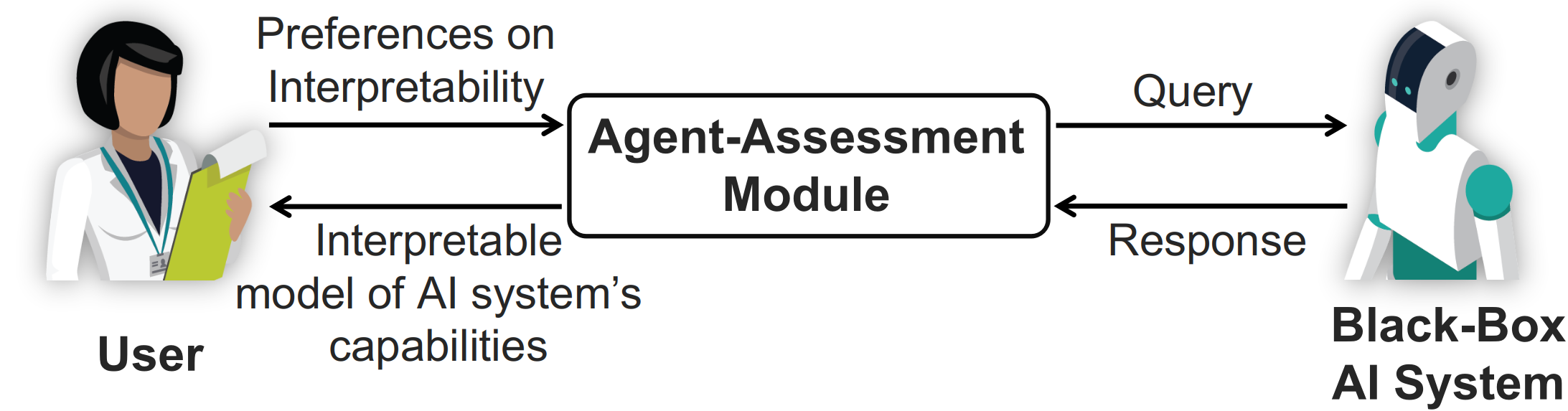
Figure 1: The agent-assessment module uses its user’s preferred vocabulary, queries the AI system, and delivers a user-interpretable causal model of the AI system’s capabilities Verma et al. (2021)

.

2.2 Causal Models

In this work, we focus on the properties of the models learned by AIA, and show that the models learned by AIA are causal. But prior to that, we must define what it means for a model to be causal. Multiple attempts have been made to define causal models Halpern and Pearl (2001, 2005); Halpern (2015). We use the definition of causal models based on Halpern (2015).

Definition 1.

A causal model $M$ is defined as a 4-tuple $\langle\mathcal{U},\mathcal{V},\mathcal{R},\mathcal{F}\rangle$ where $\mathcal{U}$ is a set of exogenous variables (representing factors outside the model’s control), $\mathcal{V}$ is a set of endogenous variables (whose values are directly or indirectly derived from the exogenous variables), $\mathcal{R}$ is a function that associates with every variable $Y\in\mathcal{U}\cup\mathcal{V}$ a nonempty set $\mathcal{R}(Y)$ of possible values for $Y$, and $\mathcal{F}$ is a function that associates with each endogenous variable $X\in\mathcal{V}$ a structural function denoted as $F_{X}$ such that $F_{X}$ maps $\times_{Z\in(\mathcal{U}\cup\mathcal{V}-\{X\})}\mathcal{R}(Z)$ to $\mathcal{R}(X)$.

Note that the values of exogenous variables are not determined by the model, and a setting $\vec{u}$ of values of exogenous variables is termed as a context by Halpern (2016). This helps in defining a causal setting as:

Definition 2.

A causal setting is a pair $(M,\vec{u})$ consisting of a causal model $M$ and context $\vec{u}$.

A causal formula $\varphi$ is true or false in a causal model, given a context. Hence, $(M,\vec{u})\models\varphi$ if the causal formula $\varphi$ is true in the causal setting $(M,\vec{u})$.

Every causal model $M$ can be associated with a directed graph, $G(M)$, in which each variable $X$ is represented as a vertex and the causal relationships between the variables are represented as directed edges between members of $\mathcal{U}\cup\{\mathcal{V}\setminus X\}$ and $X$ Pearl (2009). We use the term causal networks when referring to these graphs to avoid confusion with the notion of causal graphs used in the planning literature Helmert (2004).

To perform an analysis with interventions, we use the concept of do-calculus introduced in Pearl (1995). To perform interventions on a set of variables $X\in\mathcal{V}$, do-calculus assigns values $\vec{x}$ to $\vec{X}$, and evaluates the effect using the causal model $M$. This is termed as do($\vec{X}=\vec{x}$) action. To define this concept formally, we first define submodels Pearl (2009).

Definition 3.

Let $M$ be a causal model, $X$ a set of variables in $\mathcal{V}$, and $\vec{x}$ a particular realization of $\vec{X}$. A submodel $M_{\vec{x}}$ of $M$ is the causal model $M_{\vec{x}}=\langle\mathcal{U},\mathcal{V},\mathcal{R},\mathcal{F}^{\vec{x}}\rangle$ where $\mathcal{F}^{\vec{x}}$ is obtained from $\mathcal{F}$ by setting $X^{\prime}=x^{\prime}$ (for each $X^{\prime}\in\vec{X}$) instead of the corresponding $F_{X^{\prime}}$, and setting $F^{\vec{x}}_{Y}=F_{Y}$ for each $Y\not\in X$.

We now define what it means to intervene $\vec{X}=\vec{x}$ using the action do$(\vec{X}=\vec{x})$.

Definition 4.

Let $M$ be a causal model, $X$ a set of variables in $V$, and $\vec{x}$ a particular realization of $\vec{X}$. The effect of action do$(\vec{X}=\vec{x})$ on $M$ is given by the submodel $M_{\vec{x}}$.

In general, there can be uncertainty about the effects of these interventions, leading to probabilistic causal networks, but in this work we assume that interventions do not lead to uncertain effects.

The interventions described above assigns values to a set of variables, without affecting any another variable. Such interventions are termed as hard (independent) interventions. It is not always possible to perform such interventions and in some cases other variable(s) also change without affecting the causal structure Korb et al. (2004). Such interventions are termed as soft (dependent) interventions.

We can also derive the structure of causal networks using interventions in the real world, as interventions allow us to find if a variable $Y$ depends on another variable $X$. We use Halpern (2016)’s definition of dependence and actual cause.

Definition 5.

A variable $Y$ depends on variable $X$ if there is some setting of all the variables in $\mathcal{U}\cup\mathcal{V}\setminus\{X,Y\}$ such that varying the value of $X$ in that setting results in a variation in the value of $Y$.

Definition 6.

Given a signature $\mathcal{S}=(\mathcal{U},\mathcal{V},\mathcal{R})$, a primitive event is a formula of the form $X=x$, for $X\in\mathcal{V}$ and $x=\mathcal{R}(X)$. A causal formula is $[\vec{Y}\leftarrow\vec{y}]\varphi$, where $\varphi$ is a Boolean combination of primitive events, $\vec{Y}=\langle Y_{1},Y_{2},\dots Y_{i}\rangle$ are distinct variables in $\mathcal{V}$, and $y_{i}\in\mathcal{R}(Y_{i})$. $\varphi$ holds if $Y_{k}$ would set to $y_{k}$, for $k=1,\dots,i$.

Definition 7.

Let $X\subseteq\mathcal{V}$ be the subset of exogenous variables $\mathcal{V}$, and $\varphi$ be a boolean causal formula expressible using variables in $\mathcal{V}$. $\vec{X}=\vec{x}$ is an actual cause of $\varphi$ in the causal setting $(M,\vec{u})$, i.e., $(\vec{X}=\vec{x})\overset{(M,\vec{u})}{\lx@xy@svg{\hbox{\raise 0.0pt\hbox{\kern 3.0pt\hbox{\ignorespaces\ignorespaces\ignorespaces\hbox{\vtop{\kern 0.0pt\offinterlineskip\halign{\entry@#!@&&\entry@@#!@\cr&\crcr}}}\ignorespaces{\hbox{\kern-3.0pt\raise 0.0pt\hbox{\hbox{\kern 0.0pt\raise 0.0pt\hbox{\hbox{\kern 3.0pt\raise 0.0pt\hbox{$\textstyle{{}\ignorespaces\ignorespaces\ignorespaces\ignorespaces}$}}}}}}}\ignorespaces\ignorespaces\ignorespaces{}\ignorespaces\ignorespaces{\hbox{\lx@xy@drawsquiggles@}}\ignorespaces{\hbox{\kern 27.0pt\raise 0.0pt\hbox{\hbox{\kern 0.0pt\raise 0.0pt\hbox{\lx@xy@tip{1}\lx@xy@tip{-1}}}}}}\ignorespaces\ignorespaces{\hbox{\lx@xy@drawsquiggles@}}\ignorespaces{\hbox{\lx@xy@drawsquiggles@}}{\hbox{\kern 27.0pt\raise 0.0pt\hbox{\hbox{\kern 0.0pt\raise 0.0pt\hbox{\hbox{\kern 3.0pt\raise 0.0pt\hbox{$\textstyle{}$}}}}}}}\ignorespaces}}}}\ignorespaces}\varphi$, if the following conditions hold:

1. $(M,\vec{u})\models(\vec{X}=\vec{x})$ and $(M,\vec{u})\models\varphi$.

2. There is a set $\vec{W}$ of variables in $\mathcal{V}$ and a setting $\vec{x}^{\prime}$ of the variables in $\vec{X}$ such that if $(M,\vec{u})\models\vec{W}=\vec{w}^{*}$, then $(M,\vec{u})\models[\vec{X}\leftarrow\vec{x}^{\prime},\vec{W}\leftarrow\vec{w}^{*}]\neg\varphi$.

3. $\vec{X}$ is minimal; there is no strict subset $\vec{X}^{\prime}$ of $\vec{X}$ such that $\vec{X}^{\prime}=\vec{x}^{\prime}$ satisfies conditions AC1 and AC2, where $\vec{x}^{\prime}$ is the restriction of $\vec{x}$ to the variables in $\vec{X}$.

AC1 mentions that unless both $\varphi$ and $\vec{X}=\vec{x}$ occur at the same time, $\varphi$ cannot be caused by $\vec{X}=\vec{x}$. AC2 mentions that there exists a $\vec{x}^{\prime}$ such that if we change a subset $\vec{X}$ of variables from some initial value $\vec{x}$ to $\vec{x}^{\prime}$, keeping the value of other variables $\vec{W}$ fixed to $\vec{w}^{*}$, $\varphi$ will also change. AC3 is a minimality condition which ensures that there are no spurious elements in $\vec{X}$.

The following definition specifies soundness and completeness with respect to the actual causes entailed by a pair of causal models.

Definition 8.

Let $\vec{\mathcal{U}}$ and $\vec{\mathcal{V}}$ be the vectors of exogenous and endogenous variables, respectively; and $\Phi$ be the set of all boolean causal formulas expressible over variables in $\mathcal{V}$.

A causal model $M_{1}$ is complete with respect to another causal model $M_{2}$ if for all possible settings of exogenous variables, all the causal relationships that are implied by the model $M_{1}$ are a superset of the set of causal relationships implied by the model $M_{2}$, i.e., $\forall\vec{u}\in\vec{\mathcal{U}},\forall\vec{X},\vec{X}^{\prime}\subseteq\vec{\mathcal{V}},\forall\varphi,\varphi^{\prime}\in\Phi,\exists\vec{x}\in\vec{X},\exists\vec{x}^{\prime}\in\vec{X}^{\prime}$ s.t. $\{\langle\vec{X},\vec{u},\varphi,\vec{x}\rangle:(\vec{X}=\vec{x})\overset{(M_{2},\vec{u})}{\lx@xy@svg{\hbox{\raise 0.0pt\hbox{\kern 3.0pt\hbox{\ignorespaces\ignorespaces\ignorespaces\hbox{\vtop{\kern 0.0pt\offinterlineskip\halign{\entry@#!@&&\entry@@#!@\cr&\crcr}}}\ignorespaces{\hbox{\kern-3.0pt\raise 0.0pt\hbox{\hbox{\kern 0.0pt\raise 0.0pt\hbox{\hbox{\kern 3.0pt\raise 0.0pt\hbox{$\textstyle{{}\ignorespaces\ignorespaces\ignorespaces\ignorespaces}$}}}}}}}\ignorespaces\ignorespaces\ignorespaces{}\ignorespaces\ignorespaces{\hbox{\lx@xy@drawsquiggles@}}\ignorespaces{\hbox{\kern 27.0pt\raise 0.0pt\hbox{\hbox{\kern 0.0pt\raise 0.0pt\hbox{\lx@xy@tip{1}\lx@xy@tip{-1}}}}}}\ignorespaces\ignorespaces{\hbox{\lx@xy@drawsquiggles@}}\ignorespaces{\hbox{\lx@xy@drawsquiggles@}}{\hbox{\kern 27.0pt\raise 0.0pt\hbox{\hbox{\kern 0.0pt\raise 0.0pt\hbox{\hbox{\kern 3.0pt\raise 0.0pt\hbox{$\textstyle{}$}}}}}}}\ignorespaces}}}}\ignorespaces}\varphi\}\subseteq\{\langle\vec{X}^{\prime},\vec{u},\varphi^{\prime},\vec{x}^{\prime}\rangle:(\vec{X^{\prime}}=\vec{x^{\prime}})\overset{(M_{1},\vec{u})}{\lx@xy@svg{\hbox{\raise 0.0pt\hbox{\kern 3.0pt\hbox{\ignorespaces\ignorespaces\ignorespaces\hbox{\vtop{\kern 0.0pt\offinterlineskip\halign{\entry@#!@&&\entry@@#!@\cr&\crcr}}}\ignorespaces{\hbox{\kern-3.0pt\raise 0.0pt\hbox{\hbox{\kern 0.0pt\raise 0.0pt\hbox{\hbox{\kern 3.0pt\raise 0.0pt\hbox{$\textstyle{{}\ignorespaces\ignorespaces\ignorespaces\ignorespaces}$}}}}}}}\ignorespaces\ignorespaces\ignorespaces{}\ignorespaces\ignorespaces{\hbox{\lx@xy@drawsquiggles@}}\ignorespaces{\hbox{\kern 27.0pt\raise 0.0pt\hbox{\hbox{\kern 0.0pt\raise 0.0pt\hbox{\lx@xy@tip{1}\lx@xy@tip{-1}}}}}}\ignorespaces\ignorespaces{\hbox{\lx@xy@drawsquiggles@}}\ignorespaces{\hbox{\lx@xy@drawsquiggles@}}{\hbox{\kern 27.0pt\raise 0.0pt\hbox{\hbox{\kern 0.0pt\raise 0.0pt\hbox{\hbox{\kern 3.0pt\raise 0.0pt\hbox{$\textstyle{}$}}}}}}}\ignorespaces}}}}\ignorespaces}\varphi^{\prime}\}$.

A causal model $M_{1}$ is sound with respect to another causal model $M_{2}$ if for all possible settings of exogenous variables, all the causal relationships that are implied by the model $M_{1}$ are a subset of the set of causal relationships implied by the model $M_{2}$, i.e., $\forall\vec{u}\in\,\,\vec{\mathcal{U}},\forall\vec{X},\vec{X}^{\prime}\subseteq\vec{\mathcal{V}},\forall\varphi,\varphi^{\prime}\in\Phi,\exists\vec{x}\in\vec{X},\exists\vec{x}^{\prime}\in\vec{X}^{\prime}$ s.t. $\{\langle\vec{X},\vec{u},\varphi,\vec{x}\rangle:(\vec{X}=\vec{x})\overset{(M_{1},\vec{u})}{\lx@xy@svg{\hbox{\raise 0.0pt\hbox{\kern 3.0pt\hbox{\ignorespaces\ignorespaces\ignorespaces\hbox{\vtop{\kern 0.0pt\offinterlineskip\halign{\entry@#!@&&\entry@@#!@\cr&\crcr}}}\ignorespaces{\hbox{\kern-3.0pt\raise 0.0pt\hbox{\hbox{\kern 0.0pt\raise 0.0pt\hbox{\hbox{\kern 3.0pt\raise 0.0pt\hbox{$\textstyle{{}\ignorespaces\ignorespaces\ignorespaces\ignorespaces}$}}}}}}}\ignorespaces\ignorespaces\ignorespaces{}\ignorespaces\ignorespaces{\hbox{\lx@xy@drawsquiggles@}}\ignorespaces{\hbox{\kern 27.0pt\raise 0.0pt\hbox{\hbox{\kern 0.0pt\raise 0.0pt\hbox{\lx@xy@tip{1}\lx@xy@tip{-1}}}}}}\ignorespaces\ignorespaces{\hbox{\lx@xy@drawsquiggles@}}\ignorespaces{\hbox{\lx@xy@drawsquiggles@}}{\hbox{\kern 27.0pt\raise 0.0pt\hbox{\hbox{\kern 0.0pt\raise 0.0pt\hbox{\hbox{\kern 3.0pt\raise 0.0pt\hbox{$\textstyle{}$}}}}}}}\ignorespaces}}}}\ignorespaces}\varphi\}\subseteq\{\langle\vec{X}^{\prime},\vec{u},\varphi^{\prime},\vec{x}^{\prime}\rangle:(\vec{X^{\prime}}=\vec{x^{\prime}})\overset{(M_{2},\vec{u})}{\lx@xy@svg{\hbox{\raise 0.0pt\hbox{\kern 3.0pt\hbox{\ignorespaces\ignorespaces\ignorespaces\hbox{\vtop{\kern 0.0pt\offinterlineskip\halign{\entry@#!@&&\entry@@#!@\cr&\crcr}}}\ignorespaces{\hbox{\kern-3.0pt\raise 0.0pt\hbox{\hbox{\kern 0.0pt\raise 0.0pt\hbox{\hbox{\kern 3.0pt\raise 0.0pt\hbox{$\textstyle{{}\ignorespaces\ignorespaces\ignorespaces\ignorespaces}$}}}}}}}\ignorespaces\ignorespaces\ignorespaces{}\ignorespaces\ignorespaces{\hbox{\lx@xy@drawsquiggles@}}\ignorespaces{\hbox{\kern 27.0pt\raise 0.0pt\hbox{\hbox{\kern 0.0pt\raise 0.0pt\hbox{\lx@xy@tip{1}\lx@xy@tip{-1}}}}}}\ignorespaces\ignorespaces{\hbox{\lx@xy@drawsquiggles@}}\ignorespaces{\hbox{\lx@xy@drawsquiggles@}}{\hbox{\kern 27.0pt\raise 0.0pt\hbox{\hbox{\kern 0.0pt\raise 0.0pt\hbox{\hbox{\kern 3.0pt\raise 0.0pt\hbox{$\textstyle{}$}}}}}}}\ignorespaces}}}}\ignorespaces}\varphi^{\prime}\}$.

2.3 Query Complexity

In this paper, we provide an extended analysis of the complexity of the queries that AIA uses to learn the agent’s model. We use the complexity analysis of relational queries by Vardi [1982, 1995] to find the membership classes for data, expression, and combined complexity of AIA’s queries.

Vardi (1982) introduced three kinds of complexities for relational queries. In the notion of query complexity, a specific query is fixed in the language, then data complexity – given as function of size of databases – is found by applying this query to arbitrary databases. In the second notion of query complexity, a specific database is fixed, then the expression complexity – given as function of length of expressions – is found by studying the complexity of applying queries represented by arbitrary expressions in the language. Finally, combined complexity – given as a function of combined size of the expressions and the database – is found by applying arbitrary queries in the language to arbitrary databases.

These notions can be defined formally as follows Vardi (1995):

Definition 9.

The complexity of a query is measured as the complexity of deciding if $t\in Q(B)$, where $t$ is a tuple, $Q$ is a query, and $B$ is a database.

• The data complexity of a language $\mathcal{L}$ is the complexity of the sets $Answer(Q_{e})$ for queries $e$ in $\mathcal{L}$, where $Answer(Q_{e})$ is the answer set of a query $Q_{e}$ given as:
  $Answer(Q_{e})=\{(t,B)\,|\,t\in Q_{e}(B)\}$.

• The expression complexity of a language $\mathcal{L}$ is the complexity of the sets $Answer_{\mathcal{L}}(B)$, where $Answer_{\mathcal{L}}(B)$ is the answer set of a database $B$ with respect to a language $\mathcal{L}$ given as:
  $Answer_{\mathcal{L}}(B)=\{(t,e)\,|\,e\in\mathcal{L}\text{ and }t\in Q_{e}(B)\}$.

• The combined complexity of a language $\mathcal{L}$ is the complexity of the set $Answer_{\mathcal{L}}$, where $Answer_{\mathcal{L}}$ is the answer set of a language $\mathcal{L}$ given as:
  $Answer_{\mathcal{L}}=\{(t,B,e)\,|\,e\in\mathcal{L}\text{ and }t\in Q_{e}(B)\}$.

Vardi [1982, 1995] gave standard complexity classes for queries written in specific logical languages. We show the membership of our queries in these classes based on the logical languages we write the queries in.

3 Formal Framework

The agent assessment module assumes that the user needs to estimate the agent’s model as a STRIPS-like planning model represented as a pair $\mathcal{M}=\langle\mathbb{P},\mathbb{A}\rangle$, where $\mathbb{P}=\{p_{1}^{k_{1}},\dots,p_{n}^{k_{n}}\}$ is a finite set of predicates with arities $k_{i}$; $\mathbb{A}=\{a_{1},\dots,a_{k}\}$ is a finite set of parameterized actions (operators). Each action $a_{j}\in\mathbb{A}$ is represented as a tuple $\langle header(a_{j}),pre(a_{j}),\emph{eff}(a_{j})\rangle$, where $header(a_{j})$ is the action header consisting of action name and action parameters, $pre(a_{j})$ represents the set of predicate atoms that must be true in a state where $a_{j}$ can be applied, $\emph{eff}(a_{j})$ is the set of positive or negative predicate atoms that will change to true or false respectively as a result of execution of the action $a_{j}$. Each predicate can be instantiated using the parameters of an action, where the number of parameters are bounded by the maximum arity of the action. E.g., consider the action $\emph{load\_truck}(?v1,?v2,?v3)$ and predicate $at(?x,?y)$ in the IPC Logistics domain. This predicate can be instantiated using action parameters $?v1$, $?v2$, and $?v3$ as $at(?v1,?v1)$, $at(?v1,?v2)$, $at(?v1,?v3)$, $at(?v2,?v2)$, $at(?v2,?v1)$, $at(?v2,?v3)$, $at(?v3,?v3)$, $at(?v3,?v1)$, and $at(?v3,?v2)$. We represent the set of all such possible predicates instantiated with action parameters as $\mathbb{P}^{*}$.

AAM uses the following information as input. It receives its instruction set in the form of $header(a)$ for each $a\in\mathbb{A}$ from the agent. AAM also receives a predicate vocabulary $\mathbb{P}$ from the user with functional definitions of each predicate. This gives AAM sufficient information to perform a dialog with $\mathcal{A}$ about the outcomes of hypothetical action sequences.

We define the overall problem of agent interrogation as follows. Given a class of queries and an agent with an unknown model which can answer these queries, determine the model of the agent. More precisely, an agent interrogation task is defined as a tuple $\langle\mathcal{M}^{\mathcal{A}},\mathbb{Q},\mathbb{P},\mathbb{A}_{H}\rangle$, where $\mathcal{M}^{\mathcal{A}}$ is the true model (unknown to AAM) of the agent $\mathcal{A}$ being interrogated, $\mathbb{Q}$ is the class of queries that can be posed to the agent by AAM, and $\mathbb{P}$ and $\mathbb{A}_{H}$ are the sets of predicates and action headers that AAM uses based on inputs from $\mathcal{H}$ and $\mathcal{A}$. The objective of the agent interrogation task is to derive the agent model $\mathcal{M}^{\mathcal{A}}$ using $\mathbb{P}$ and $\mathbb{A}_{H}$. Let $\Theta$ be the set of possible answers to queries. Thus, strings $\theta^{*}\in\Theta^{*}$ denote the information received by AAM at any point in the query process. Query policies for the agent interrogation task are functions $\Theta^{*}\rightarrow\mathbb{Q}\cup\{\emph{Stop}\}$ that map sequences of answers to the next query that the interrogator should ask. The process stops with the Stop query. In other words, for all answers $\theta\in\Theta$, all valid query policies map all sequences $x\theta$ to Stop whenever $x\in\Theta^{*}$ is mapped to Stop. This policy is computed and executed online.

Running Example    Consider we have a driving robot having a single action drive (?t ?s ?d), parameterized by the truck it drives, source location, and destination location. Assume that all the locations are connected, hence the robot can drive between any two locations. The predicates available are $at(?t\,\,?loc)$, representing the location of a truck; and $src\_blue(?loc)$, representing the color of the source location. Instantiating $at$ and $src\_blue$ with parameters of the action drive gives four instantiated predicates $at(?t\,\,?s)$, $at(?t\,\,?d)$, $src\_blue(?s)$, and $src\_blue(?d)$.

4 Learning Causal Models

The classic causal model framework used in Def. 1 lacks the temporal elements and decision nodes needed to express the causality in planning domains.

To express actions, we use the decision nodes similar to Dynamic Decision Networks Kanazawa and Dean (1989). To express the temporal behavior of planning models, we use the notion of Dynamic Causal Models Pearl (2009) and Dynamic Causal Networks (DCNs) Blondel et al. (2017). These are similar to causal models and causal networks respectively, with the only difference that the variables in these are time-indexed, allowing for analysis of temporal causal relations between the variables. We also introduce additional boolean variables to capture the executability of the actions. The resulting causal model is termed as a causal action model, and we express such models using a Dynamic Causal Decision Network (DCDN).

A general structure of a dynamic causal decision network is shown in Fig.​ 2. Here $s_{t}$ and $s_{t+1}$ are states at time $t$ and $t+1$ respectively, $a_{t}$ is a decision node representing the decision to execute action $a$ at time $t$, and executability variable $X^{a}_{t}$ represents if action $a$ is executable at time $t$. All the decision variables and the executability variables $X_{t}^{a}$, where $a\in\mathbb{A}$, in a domain are endogenous. Decision variables are endogenous because we can perform interventions on them as needed.

4.1 Types of Interventions

To learn the causal action model corresponding to each domain, two kinds of interventions are needed. The first type of interventions, termed $\mathcal{I}_{P}$, correspond to searching for the initial state in AIA. AIA searches for the state where it can execute an action, hence if the state variables are completely independent of each other, these interventions are hard, whereas for the cases where some of the variables are dependent the interventions are soft for those variables. Such interventions lead to learning the preconditions of an action correctly.

The second type of interventions, termed $\mathcal{I}_{E}$, are on the decision nodes, where the values of the decision variables are set to true according to the input plan. For each action $a_{i}$ in the plan $\pi$, the corresponding decision node with label $a_{i}$ is set to true. Of course, during the intervention process, the structure of the true DCDN is not known. Such interventions lead to learning the effects of an action accurately. As mentioned earlier, if an action $a$ is executed in a state $s_{t}$ which does not satisfy its preconditions, the variable $X^{a}_{t}$ will be false at that time instant, and the resulting state $s_{t+1}$ will be same as state $s_{t}$, signifying a failure to execute the action. Note that the state nodes $s_{t}$ and $s_{t+1}$ in Fig.​ 2 are the combined representation of multiple predicates.

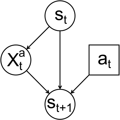
Figure 2: An example of a Dynamic Causal Decision Network (DCDN). $s_{t}$ and $s_{t+1}$ are states at time $t$ and $t+1$ respectively, $a_{t}$ is a decision node representing the decision to execute action $a$ at time $t$, and $X^{a}_{t}$ represents if action $a$ is executable at time $t$.

We now show that the model(s) learned by AIA are causal models.

Lemma 1.

Given an agent $\mathcal{A}$ with a ground truth model $M^{\mathcal{A}}$ (unknown to the agent interrogation algorithm AIA), the action model $M$ learned by AIA is a causal model consistent with Def. 1.

Proof (Sketch).

We show a mapping between the components of the causal models used in Def. 1 and the planning models described in Sec.​ 3. The exogenous variables $\mathcal{U}$ maps to the static predicates in the domain, i.e., the ones that do not appear in the effect of any action; $\mathcal{V}$ maps to the non-static predicates; $\mathcal{R}$ maps each predicate to $\top$ if the predicate is true in a state, or $\bot$ when the predicate is false in a state; $\mathcal{F}$ calculates the value of each variable depending on the other variables that cause it. This is captured by the values of state predicates and executability variables being changed due to other state variables and decision variables.

The causal relationships in the model $\mathcal{M}$ learned by AIA also satisfy the three conditions – AC1, AC2, and AC3 – mentioned in the definition for the actual cause (Def. 7). By Thm.​ 1 in Verma et al. (2021), AIA returns correct models, i.e., $\mathcal{M}$ contains exactly the same palm tuples as $\mathcal{M}^{\mathcal{A}}$.

This also means that AC1 is satisfied due to correctness of $\mathcal{I}_{P}$ – a predicate $p$ is a cause of $X^{a}$ only when $p$ is precondition of action $a$; and $\mathcal{I}_{E}$– a predicate $p$ is a caused by $X^{a}$ and $a$ only when $p$ is an effect of action $a$. AC2 is satisfied because if any precondition of an action is not satisfied, it will not execute (defining the relationship “state variables $\rightarrow X^{a}$”); or if any action doesn’t execute, it won’t affect the predicates in its effects (defining the relationship “$X^{a}\rightarrow$ state variables”). Finally, AC3 is satisfied, as neither spurious preconditions are learned by AIA, nor incorrect effects are learned. ∎

We now formally show that the causal model(s) learned by AIA is(are) sound and complete.

Theorem 1.

Given an agent $\mathcal{A}$ with a ground truth model $M^{\mathcal{A}}$ (unknown to the agent interrogation algorithm AIA), the action model $M$ learned by AIA is sound and complete with respect to $M^{\mathcal{A}}$.

Proof (Sketch).

We first show that $M$ is sound with respect to $M^{\mathcal{A}}$. Assume that some $\vec{X}=\vec{x}$ is an actual cause of $\varphi$ according to $M$ in the setting $\vec{u}$, i.e., $(\vec{X}=\vec{x})\overset{(M,\vec{u})}{\lx@xy@svg{\hbox{\raise 0.0pt\hbox{\kern 3.0pt\hbox{\ignorespaces\ignorespaces\ignorespaces\hbox{\vtop{\kern 0.0pt\offinterlineskip\halign{\entry@#!@&&\entry@@#!@\cr&\crcr}}}\ignorespaces{\hbox{\kern-3.0pt\raise 0.0pt\hbox{\hbox{\kern 0.0pt\raise 0.0pt\hbox{\hbox{\kern 3.0pt\raise 0.0pt\hbox{$\textstyle{{}\ignorespaces\ignorespaces\ignorespaces\ignorespaces}$}}}}}}}\ignorespaces\ignorespaces\ignorespaces{}\ignorespaces\ignorespaces{\hbox{\lx@xy@drawsquiggles@}}\ignorespaces{\hbox{\kern 27.0pt\raise 0.0pt\hbox{\hbox{\kern 0.0pt\raise 0.0pt\hbox{\lx@xy@tip{1}\lx@xy@tip{-1}}}}}}\ignorespaces\ignorespaces{\hbox{\lx@xy@drawsquiggles@}}\ignorespaces{\hbox{\lx@xy@drawsquiggles@}}{\hbox{\kern 27.0pt\raise 0.0pt\hbox{\hbox{\kern 0.0pt\raise 0.0pt\hbox{\hbox{\kern 3.0pt\raise 0.0pt\hbox{$\textstyle{}$}}}}}}}\ignorespaces}}}}\ignorespaces}\varphi$. Now by Thm.​ 1 in Verma et al. (2021), $\mathcal{M}$ contains exactly the same palm tuples as $\mathcal{M}^{\mathcal{A}}$. Hence any palm tuple that is present in $M$ will also be present in $M^{\mathcal{A}}$, implying that under the same setting $\vec{u}$ according to $M^{\mathcal{A}}$ $\vec{X}=\vec{x}$ is an actual cause of $\varphi$.

Now lets assume that some $\vec{X}=\vec{x}$ is an actual cause of $\varphi$ according to $M^{\mathcal{A}}$ in the setting $\vec{u}$, i.e., $(\vec{X}=\vec{x})\overset{(M^{\mathcal{A}},\vec{u})}{\lx@xy@svg{\hbox{\raise 0.0pt\hbox{\kern 3.0pt\hbox{\ignorespaces\ignorespaces\ignorespaces\hbox{\vtop{\kern 0.0pt\offinterlineskip\halign{\entry@#!@&&\entry@@#!@\cr&\crcr}}}\ignorespaces{\hbox{\kern-3.0pt\raise 0.0pt\hbox{\hbox{\kern 0.0pt\raise 0.0pt\hbox{\hbox{\kern 3.0pt\raise 0.0pt\hbox{$\textstyle{{}\ignorespaces\ignorespaces\ignorespaces\ignorespaces}$}}}}}}}\ignorespaces\ignorespaces\ignorespaces{}\ignorespaces\ignorespaces{\hbox{\lx@xy@drawsquiggles@}}\ignorespaces{\hbox{\kern 27.0pt\raise 0.0pt\hbox{\hbox{\kern 0.0pt\raise 0.0pt\hbox{\lx@xy@tip{1}\lx@xy@tip{-1}}}}}}\ignorespaces\ignorespaces{\hbox{\lx@xy@drawsquiggles@}}\ignorespaces{\hbox{\lx@xy@drawsquiggles@}}{\hbox{\kern 27.0pt\raise 0.0pt\hbox{\hbox{\kern 0.0pt\raise 0.0pt\hbox{\hbox{\kern 3.0pt\raise 0.0pt\hbox{$\textstyle{}$}}}}}}}\ignorespaces}}}}\ignorespaces}\varphi$. Now by Thm.​ 1 in Verma et al. (2021), $\mathcal{M}$ contains exactly the same palm tuples as $\mathcal{M}^{\mathcal{A}}$. Hence any palm tuple that is present in $M^{a}g$ will also be present in $M$, implying that under the same setting $\vec{u}$ according to $M$ $\vec{X}=\vec{x}$ is an actual cause of $\varphi$. Hence the action model $M$ learned by the agent interrogation algorithm are sound and complete with respect to the model $M^{\mathcal{A}}$. ∎

4.2 Comparison with Observational Data based Learners

We compare the properties of models learned by AIA with those of approaches that learn the models from observational data only. For the methods that learn models in STRIPS-like the learned models can be classified as causal, but it is not necessary that they are sound with respect to the ground truth model $M^{\mathcal{A}}$ of the agent $\mathcal{A}$. E.g., in case of the robot driver discussed earlier, these methods can learn a model where the precondition of the action drive is $src\_blue$ if all the observation traces that are provided to it as input had $src\_blue$ as true. This can happen if all the source locations are painted blue. To avoid such cases, some of these methods run a pre-processing or a post-processing step that removes all static predicates from the preconditions. However, if there is a paint action in the domain that changes the color of all source locations, then these ad-hoc solutions will not be able to handle that. Hence, these techniques may end up learning spurious preconditions as they do not have a way to distinguish between correlation and causations.

On the other hand, it is also not necessary that the models learned by approaches using only observational data are complete with respect to the ground truth model $M^{\mathcal{A}}$ of the agent $\mathcal{A}$. This is because they may miss to capture some causal relationships if the observations do not include all the possible transitions, or contains only the successful actions. E.g., if we have additional predicates $city\_from(?loc)$, and $city\_to(?loc)$ in the domain, and all the observed transitions are for the transitions within same city, then the model will not be able to learn if the source city and destination city have to be same for driving a truck between them.

Hence, the models learned using only observational data are not necessarily sound or complete, as they can learn causal relationships that are not part of set of actual causal relationships, and can also miss some of the causal relationships that are not part of set of actual causal relationships. Pearl (2019) also points out that it is not possible to learn causal models from observational data only.

4.3 Types of Queries

Plan Outcome Queries    Verma et al. (2021) introduced plan outcome queries $\mathcal{Q}_{PO}$, which are parameterized by a state $s_{I}$ and a plan $\pi$. Let $P$ be the set of predicates $\mathbb{P}^{*}$ instantiated with objects $O$ in an environment. $\mathcal{Q}_{PO}$ queries ask $\mathcal{A}$ the length of the longest prefix of the plan $\pi$ that it can execute successfully when starting in the state $s_{I}\subseteq P$ as well as the final state $s_{F}\subseteq P$ that this execution leads to. E.g., “Given that the truck $t1$ is at location $l1$, what would happen if you executed the plan $\langle drive(t1,l1,l2)$, $drive(t1,l2,l3)$, $drive(t1,l2,l1)\rangle$?”

A response to such queries can be of the form “I can execute the plan till step $\ell$ and at the end of it truck $t1$ is at location $l3$”. Formally, the response $\theta_{PO}$ for plan outcome queries is a tuple $\langle\ell,s_{\ell}\rangle$, where $\ell$ is the number of steps for which the plan $\pi$ could be executed, and $s_{\ell}\subseteq P$ is the final state after executing $\ell$ steps of the plan. If the plan $\pi$ cannot be executed fully according to the agent model $\mathcal{M}^{\mathcal{A}}$ then $\ell<len(\pi)$, otherwise $\ell=len(\pi)$. The final state $s_{\ell}\subseteq P$ is such that $\mathcal{M}^{\mathcal{A}}\models\pi{[1:\ell]}(s_{I})=s_{\ell}$, i.e., starting from a state $s_{I}$, $\mathcal{M}^{\mathcal{A}}$ successfully executed first $\ell$ steps of the plan $\pi$. Thus, $\mathcal{Q}_{PO}:\mathcal{U}\rightarrow\mathbb{N}\times 2^{P}$, where $\mathcal{U}$ is the set of all the models that can be generated using the predicates $P$ and actions $\mathbb{A}$, and $\mathbb{N}$ is the set of natural numbers.

Action Precondition Queries    In this work, we introduce a new class of queries called action precondition queries $\mathcal{Q}_{AP}$. These queries, similar to plan outcome queries, are parameterized by $s_{I}$ and $\pi$, but have a different response type.

A response to the action precondition queries can be either of the form “I can execute the plan completely and at the end of it, truck $t1$ is at location $l1$” when the plan is successfully executed, or of the form “I can execute the plan till step $\ell$ and the action $a_{\ell}$ failed because precondition $p_{i}$ was not satisfied” when the plan is not fully executed. To make the responses consistent in all cases, we introduce a dummy action $a_{\emph{fail}}$ whose precondition is never satisfied. Hence, the responses are always of the form, “I can execute the plan till step $\ell$ and the action $a_{\ell}$ failed because precondition $p_{F}$ was not satisfied”. If $a_{\ell}$ is $a_{\emph{fail}}$ and $\ell=len(\pi)$, then we know that the original plan was executed successfully by the agent. Formally, the response $\theta_{AP}$ for action precondition queries is a tuple $\langle\ell,p_{F}\rangle$, where $\ell$ is the number of steps for which the plan $\pi$ could be executed, and $p_{F}\subseteq P$ is the set of preconditions of the failed action $a_{F}$. If the plan $\pi$ cannot be executed fully according to the agent model $\mathcal{M}^{\mathcal{A}}$ then $\ell<len(\pi)-1$, otherwise $\ell=len(\pi)-1$. Also, $\mathcal{Q}_{AC}:\mathcal{U}\rightarrow\mathbb{N}\times P$, where $\mathcal{U}$ is the set of all the models that can be generated using the predicates $P$ and actions $\mathbb{A}$, and $\mathbb{N}$ is the set of natural numbers.

5 Complexity Analysis

Theoretically, the asymptotic complexity of AIA (with plan outcome queries) is $O(|\mathbb{P}^{*}|\times|\mathbb{A}|)$, but it does not take into account how much computation is needed to answer the queries, or to evaluate their responses. This complexity just shows the amount of computation needed in the worst case to derive the agent model by AIA. Here, we present a more detailed analysis of the complexity of AIA’s queries using the results of relational query complexity by Vardi (1982).

To analyze $\mathcal{Q}_{PO}$’s complexity, let us assume that the agent has stored the possible transitions it can make (in propositional form) using the relations $R(\emph{valid},s,a,s^{\prime},\emph{succ})$, where $\emph{valid},\emph{succ}\in\{\top,\bot\}$, $s,s^{\prime}\in S$, $a\in A$; and $N(\emph{valid},n,n_{+})$, where $\emph{valid}\in\{\top,\bot\}$, $n,n_{+}\in\mathbb{N}$, $0\leq n\leq L$, and $0\leq n_{+}\leq L+1$, where $L$ is the maximum possible length of a plan in the $\mathcal{Q}_{PO}$ queries. $L$ can be an arbitrarily large number, and it does not matter as long as it is finite. Here, $S$ and $A$ are sets of grounded states and actions respectively. $succ$ is $\top$ if the action was executed successfully, and is $\bot$ if the action failed. $valid$ is $\top$ when none of the previous actions had $succ=\bot$. This stops an action to change a state if any of the previous actions failed, thereby preserving the state that resulted from a failed action. Whenever $succ=\bot$ or $valid=\bot$, $s=s^{\prime}$ and $n=n_{+}$ signifying that applying an action where it is not applicable does not change the state.

Assuming the length of the query plan, $len(\pi)=D$, we can write a query in first order logic, equivalent to the plan outcome query as

$$\{(s_{D}, n_{D})\,|\,\,\exists s_{1},\dots,\exists s_{D-1},\exists succ_{1},\dots,\exists succ_{D-1},$$

$$\exists n_{1},\dots,\exists n_{D-1}R(\top,s_{0},a_{1},s_{1},succ_{1})\land$$

$$R(succ_{1},s_{1},a_{2},s_{2},succ_{2})\land\dots\land$$

$$R(succ_{D-1},s_{D-1},a_{D},s_{D},\top)\land$$

$$N(\top,0,n_{1})\land N(succ_{1},n_{1},n_{2})\land\dots\land$$

$$N(succ_{D-1},n_{D-1},n_{D})\}$$

The output of the query contains the free variables $s_{D}=s_{\ell}$ and $n_{D}=\ell$. Such first order (FO) queries have the expression complexity and the combined complexity in PSPACE Vardi (1982). The data complexity class of FO queries is $AC^{0}$ Immerman (1987).

The following results use the analysis in Vardi (1995). The query analysis given above depends on how succinctly we can express the queries. In the FO query shown above, we have a lot of spurious quantified variables. We can reduce its complexity by using bounded-variable queries. Normally, queries in a language $\mathcal{L}$ assume an inifinite supply $x_{1},x_{2},\dots$ of individual variables. A bounded-variable version $\mathcal{L}^{k}$ of the language $\mathcal{L}$ is one which can be obtained by restricting the individual variables to be among $x_{1},\dots,x_{k}$, for $k>0$. Using this, we can reduce the quantified variables in $FO$ query shown earlier, and rewrite it more succinctly as an $FO^{k}$ query by storing temporary query outputs.

$$E(succ,s,a,s^{\prime},succ^{\prime},n,n^{\prime})\!= R(succ,s,a,s^{\prime},succ^{\prime})\land$$

$$N(succ,n,n^{\prime})$$

$$\alpha_{1}(succ,s,a_{1},s^{\prime},succ^{\prime},n,n^{\prime})\!= E(\top,s_{0},a_{1},s^{\prime},succ^{\prime},0,n^{\prime})$$

We then write subsequent queries corresponding to each step of the query plan as

$$\alpha_{i+1}( succ,s,a_{i+1},s^{\prime},succ^{\prime},n,n^{\prime})=$$

$$\exists s_{1},\exists succ_{1},\exists n_{1}\{E(succ,s,a_{i+1},s_{1},succ_{1},n_{1})\land$$

$$\hskip 14.45377pt\exists s,\exists succ,\exists n[succ=succ_{1}\land s=s_{1}\land$$

$$\hskip 21.68121ptn=n_{1}\land\alpha_{i}(succ,s,a_{i},s^{\prime},succ^{\prime},n,n^{\prime})]\}$$

Here $i$ varies from $1$ to $D$, and the value of $k$ is 6 because of 6 quantified variables – $s,s_{1},succ,succ_{1},n,$ and $n_{1}$. This reduces the expression and combined complexity of these queries to ALOGTIME and PTIME respectively. Note that these are the membership classes as it might be possible to write the queries more succinctly.

For a detailed analysis of $\mathcal{Q}_{AP}$’s complexity, let us assume that the agent stores the possible transitions it can make (in propositional form) using the relations $R(\emph{valid},s,a,s^{\prime},\emph{succ})$, where $\emph{valid},\emph{succ}\in\{\top,\bot\}$, $s,s^{\prime}\in S$, $a\in A$; and $\mathcal{S}(p,s)$, where $p\in P$, $s\in S$. $\mathcal{S}$ contains $(p,s)$ if a grounded predicate $p$ is in state $s$.

Now, we can write a query in first order logic, equivalent to the action precondition query as:

$$\{(p)\,|\,\, (\forall s_{1}\,\mathcal{S}(p,s_{1})\Rightarrow\exists s^{\prime}R(\top,s_{1},a_{1},s^{\prime},\top))\,\,\land$$

$$(\forall s_{1}\,\neg\mathcal{S}(p,s_{1})\Rightarrow\forall s^{\prime}R(\top,s_{1},a_{1},s^{\prime},\bot))\}$$

This formulation is equivalent to the $FO^{k}$ queries with $k=2$. This means that the data, expression and combined complexity of these queries are in complexity classes AC⁰, ALOGTIME, and PTIME respectively.

The results for complexity classes of the queries presented above holds assuming that the agent stores all the transitions using a mechanism equivalent to relational databases where it can search through states in linear time. For the simulator agents that we generally encounter, this assumption almost never holds true. Even though both the queries have membership in the same complexity class, an agent will have to spend more time in running the action precondition query owing to the exhaustive search of all the states in all the cases, whereas for the plan outcome queries, the exhaustive search is not always needed.

Additionally, plan outcome queries place very little requirements on the agent to answer the queries, whereas action precondition queries require an agent to use more computation to generate it’s responses. Action precondition queries also force an agent to know all the transitions beforehand. So if an agent does not know its model but has to execute an action in a state to learn the transition, action precondition queries will perform poorly as agent will execute that action in all possible states to answer the query. On the other hand, to answer plan outcome queries in such cases, an agent will have to execute at most L actions (maximum length of the plan) to answer a query.

Evaluating the responses of queries will be much easier for the action precondition queries, whereas evaluating the responses of plan outcome queries is not straightforward, as discussed in Verma et al. (2021). As mentioned earlier, the agent interrogation algorithm that uses the plan outcome queries has asymptotic complexity $O(|\mathbb{P}^{*}|\times|\mathbb{A}|)$ for evaluating all agent responses. On the other hand, if an algorithm is implemented with action precondition queries, its asymptotic complexity for evaluating all agent responses will reduce to $O(|\mathbb{A}|)$. This is because AAM needs to ask two queries for each action. The first query in a state where it is guaranteed that the action will fail, this will lead AAM to learn the action’s precondition. After that AAM can ask another query in a state where the action will not fail, and learn the action’s effects. This will also lead to an overall less number of queries.

So there is a tradeoff between the computation efforts needed for evaluation of query responses and the computational burden on the agent to answer those queries.

6 Empirical Evaluation

We implemented AIA with plan outcome queries in Python to evaluate the efficacy of our approach. In this implementation, initial states were collected by making the agent perform random walks in a simulated environment. We used a maximum of 60 such random initial states for each domain in our experiments. The implementation is optimized to store the agent’s answers to queries; hence the stored responses are used if a query is repeated.

We tested AIA on two types of agents: symbolic agents that use models from the IPC (unknown to AIA), and simulator agents that report states as images using PDDLGym Silver and Chitnis (2020). All experiments were executed on 5.0 GHz Intel i9-9900 CPUs with 64 GB RAM running Ubuntu 18.04.

The analysis presented below shows that AIA learns the correct model with a reasonable number of queries, and compares our results with the closest related work, FAMA Aineto et al. (2019). We use the metric of model accuracy in the following analysis: the number of correctly learned palm tuples normalized with the total number of palm tuples in $\mathcal{M}^{\mathcal{A}}$.

6.1 Experiments with symbolic agents

We initialized the agent with one of the 10 IPC domain models, and ran AIA on the resulting agent. 10 different problem instances were used to obtain average performance estimates.

Table 1 shows that the number of queries required increases with the number of predicates and actions in the domain. We used Fast Downward Helmert (2006) with LM-Cut heuristic Helmert and Domshlak (2009) to solve the planning problems. Since our approach is planner-independent, we also tried using FF Hoffmann and Nebel (2001) and the results were similar. The low variance shows that the method is stable across multiple runs.

Domain	$\mathbf{|\mathbb{P}^{*}|}$	$\mathbf{|\mathbb{A}|}$	$\mathbf{|\hat{\mathcal{Q}}|}$	$\mathbf{t_{\mu}}$ (ms)	$\mathbf{t_{\sigma}}$ ($\mathbf{\mu}$s)
Gripper	5	3	17	18.0	0.2
Blocksworld	9	4	48	8.4	36
Miconic	10	4	39	9.2	1.4
Parking	18	4	63	16.5	806
Logistics	18	6	68	24.4	1.73
Satellite	17	5	41	11.6	0.87
Termes	22	7	134	17.0	110.2
Rovers	82	9	370	5.1	60.3
Barman	83	17	357	18.5	1605
Freecell	100	10	535	2.24†	33.4†

Table 1: The number of queries ($|\hat{\mathcal{Q}}|$), average time per query ($t_{\mu}$), and variance of time per query ($t_{\sigma}$) generated by AIA with FD. Average and variance are calculated for 10 runs of AIA, each on a separate problem. ^†Time in sec.

6.1.1 Comparison with FAMA

We compare the performance of AIA with that of FAMA in terms of stability of the models learned and the time taken per query. Since the focus of our approach is on automatically generating useful traces, we provided FAMA randomly generated traces of length 3 (the length of the longest plans in AIA-generated queries) of the form used throughout this paper ($\langle s_{I},a_{1},a_{2},a_{3},s_{G}\rangle$).

Fig. 3 summarizes our findings. AIA takes lesser time per query and shows better convergence to the correct model. FAMA sometimes reaches nearly accurate models faster, but its accuracy continues to oscillate, making it difficult to ascertain when the learning process should be stopped (we increased the number of traces provided to FAMA until it ran out of memory). This is because the solution to FAMA’s internal planning problem introduces spurious palm tuples in its model if the input traces do not capture the complete domain dynamics. For Logistics, FAMA generated an incorrect planning problem, whereas for Freecell and Barman it ran out of memory (AIA also took considerable time for Freecell). Also, in domains with negative preconditions like Termes, FAMA was unable to learn the correct model. We used Madagascar Rintanen (2014) with FAMA as it is the preferred planner for it. We also tried FD and FF with FAMA, but as the original authors noted, it could not scale and ran out of memory on all but a few Blocksworld and Gripper problems where it was much slower than with Madagascar.

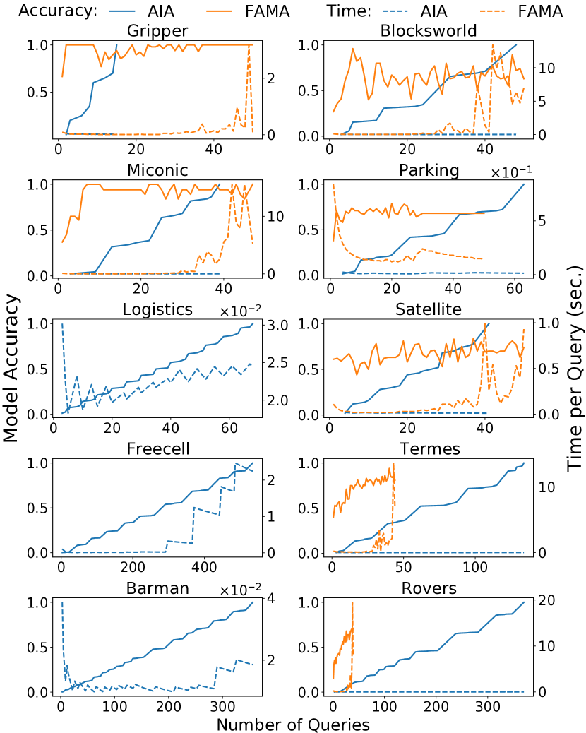
Figure 3: Performance comparison of AIA and FAMA in terms of model accuracy and time taken per query with an increasing number of queries.

6.2 Experiments with simulator agents

AIA can also be used with simulator agents that do not know about predicates and report states as images. To test this, we wrote classifiers for detecting predicates from images of simulator states in the PDDLGym framework. This framework provides ground-truth PDDL models, thereby simplifying the estimation of accuracy. We initialized the agent with one of the two PDDLGym environments, Sokoban and Doors. AIA inferred the correct model in both cases and the number of instantiated predicates, actions, and the average number of queries (over 5 runs) used to predict the correct model for Sokoban were 35, 3, and 201, and that for Doors were 10, 2, and 252.

7 Related Work

One of the ways most current techniques learn the agent models is based on passive or active observations of the agent’s behavior, mostly in the form of action traces Gil (1994); Yang et al. (2007); Cresswell et al. (2009); Zhuo and Kambhampati (2013). Jiménez et al. (2012) and Arora et al. (2018) present comprehensive review of such approaches. FAMA Aineto et al. (2019) reduces model recognition to a planning problem and can work with partial action sequences and/or state traces as long as correct initial and goal states are provided. While FAMA requires a post-processing step to update the learnt model’s preconditions to include the intersection of all states where an action is applied, it is not clear that such a process would necessarily converge to the correct model. Our experiments indicate that such approaches exhibit oscillating behavior in terms of model accuracy because some data traces can include spurious predicates, which leads to spurious preconditions being added to the model’s actions. As we mentioned earlier, such approaches do not feature interventions, and hence the models learned by these techniques do not capture causal relationships correctly and feature correlations.

Pearl (2019) introduce a 3-level causal hierarchy in terms of the classification of causal information in terms of the type of questions each class can answer. He also notes that based on passive observations alone, only associations can be learned, not the interventional or counterfactual causal relationships, regardless of the size of data.

The field of active learning Settles (2012) addresses the related problem of selecting which data-labels to acquire for learning single-step decision-making models using statistical measures of information. However, the effective feature set here is the set of all possible plans, which makes conventional methods for evaluating the information gain of possible feature labelings infeasible. In contrast, our approach uses a hierarchical abstraction to select queries to ask, while inferring a multistep decision-making (planning) model. Information-theoretic metrics could also be used in our approach whenever such information is available.

Blondel et al. (2017) introduced Dynamical Causal Networks which extend the causal graphs to temporal domains, but they do not feature decision variables, which we introduce in this paper.

8 Conclusion

We introduced dynamic causal decision networks (DCDNs) to represent causal structures in STRIPS-like domains; and showed that the models learned using the agent interrogation algorithm are causal, and are sound and complete with respect to the corresponding unknown ground truth models. We also presented an extended analysis of the queries that can be asked to the agents to learn their model, and the requirements and capabilities of the agents to answer those queries.

Extending the empirical analysis to action precondition queries, and extending our predicate classifier to handle noisy state detection, similar to prevalent approaches using classifiers to detect symbolic states Konidaris et al. (2014); Asai and Fukunaga (2018) are a few good directions for future work. Some other promising extensions include replacing query and response communication interfaces between the agent and AAM with a natural language similar to Lindsay et al. (2017), or learning other representations like Zhuo et al. (2014).

References

- Aineto et al. [2019] Diego Aineto, Sergio Jiménez Celorrio, and Eva Onaindia. Learning Action Models With Minimal Observability. Artificial Intelligence, 275:104–137, 2019.
- Arora et al. [2018] Ankuj Arora, Humbert Fiorino, Damien Pellier, Marc Métivier, and Sylvie Pesty. A Review of Learning Planning Action Models. The Knowledge Engineering Review, 33:E20, 2018.
- Asai and Fukunaga [2018] Masataro Asai and Alex Fukunaga. Classical Planning in Deep Latent Space: Bridging the Subsymbolic-Symbolic Boundary. In Proc. AAAI, 2018.
- Blondel et al. [2017] Gilles Blondel, Marta Arias, and Ricard Gavaldà. Identifiability and Transportability in Dynamic Causal Networks. International Journal of Data Science and Analytics, 3(2):131–147, 03 2017.
- Cresswell et al. [2009] Stephen Cresswell, Thomas McCluskey, and Margaret West. Acquisition of Object-Centred Domain Models from Planning Examples. In Proc. ICAPS, 2009.
- Fikes and Nilsson [1971] Richard E Fikes and Nils J Nilsson. STRIPS: A New Approach to the Application of Theorem Proving to Problem Solving. Artificial Intelligence, 2(3-4):189–208, 1971.
- Fox and Long [2003] Maria Fox and Derek Long. PDDL2.1: An Extension to PDDL for Expressing Temporal Planning Domains. Journal of Artificial Intelligence Research, 20(1):61–124, 2003.
- Gil [1994] Yolanda Gil. Learning by Experimentation: Incremental Refinement of Incomplete Planning Domains. In Proc. ICML, 1994.
- Halpern and Pearl [2001] Joseph Y Halpern and Judea Pearl. Causes and Explanations: A Structural-Model Approach. Part I: Causes. In Proc. UAI, 2001.
- Halpern and Pearl [2005] Joseph Y Halpern and Judea Pearl. Causes and Explanations: A Structural-Model Approach. Part I: Causes. The British journal for the philosophy of science, 56(4):843–887, 2005.
- Halpern [2015] Joseph Y. Halpern. A Modification of the Halpern-Pearl Definition of Causality. In Proc. IJCAI, 2015.
- Halpern [2016] Joseph Y. Halpern. Actual Causality. The MIT Press, 2016.
- Helmert and Domshlak [2009] M. Helmert and C. Domshlak. Landmarks, Critical Paths and Abstractions: What’s the Difference Anyway? In Proc. ICAPS, 2009.
- Helmert [2004] Malte Helmert. A Planning Heuristic Based on Causal Graph Analysis. In Proc. ICAPS, 2004.
- Helmert [2006] Malte Helmert. The Fast Downward Planning System. Journal of Artificial Intelligence Research, 26:191–246, 2006.
- Hoffmann and Nebel [2001] Jörg Hoffmann and Bernhard Nebel. The FF Planning System: Fast Plan Generation Through Heuristic Search. Journal of Artificial Intelligence Research, 14:253–302, 2001.
- Immerman [1987] Neil Immerman. Expressibility as a complexity measure: Results and directions. Technical Report YALEU/DCS/TR-538, Department of Computer Science, Yale University, 1987.
- Jiménez et al. [2012] Sergio Jiménez, Tomás De La Rosa, Susana Fernández, Fernando Fernández, and Daniel Borrajo. A Review of Machine Learning for Automated Planning. The Knowledge Engineering Review, 27(4):433–467, 2012.
- Kanazawa and Dean [1989] Keiji Kanazawa and Thomas Dean. A Model for Projection and Action. In Proc. IJCAI, 1989.
- Konidaris et al. [2014] George Konidaris, Leslie Pack Kaelbling, and Tomas Lozano-Perez. Constructing Symbolic Representations for High-Level Planning. In Proc. AAAI, 2014.
- Korb et al. [2004] Kevin B. Korb, Lucas R. Hope, Ann E. Nicholson, and Karl Axnick. Varieties of Causal Intervention. In Proc. PRICAI: Trends in Artificial Intelligence, 2004.
- Lindsay et al. [2017] Alan Lindsay, Jonathon Read, João Ferreira, Thomas Hayton, Julie Porteous, and Peter Gregory. Framer: Planning Models from Natural Language Action Descriptions. In Proc. ICAPS, 2017.
- McDermott et al. [1998] Drew McDermott, Malik Ghallab, Adele Howe, Craig Knoblock, A. Ram, Manuela Veloso, Daniel S. Weld, and David Wilkins. PDDL – The Planning Domain Definition Language. Technical Report CVC TR-98-003/DCS TR-1165, Yale Center for Computational Vision and Control, 1998.
- Pearl [1995] Judea Pearl. Causal Diagrams for Empirical Research. Biometrika, 82(4):669–688, 1995.
- Pearl [2009] Judea Pearl. Causality: Models, Reasoning, and Inference. Cambridge University Press, 2009.
- Pearl [2019] Judea Pearl. The Seven Tools of Causal Inference, with Reflections on Machine Learning. Communications of the ACM, 62(3):54–60, 2019.
- Rintanen [2014] Jussi Rintanen. Madagascar: Scalable Planning with SAT. In Proc. 8th International Planning Competition., 2014.
- Settles [2012] Burr Settles. Active Learning. Morgan & Claypool Publishers, 2012.
- Silver and Chitnis [2020] Tom Silver and Rohan Chitnis. PDDLGym: Gym Environments from PDDL Problems. In ICAPS Workshop on Bridging the Gap Between AI Planning and Reinforcement Learning (PRL), 2020.
- Srivastava [2021] Siddharth Srivastava. Unifying Principles and Metrics for Safe and Assistive AI. In Proc. AAAI, 2021.
- Vardi [1982] Moshe Y. Vardi. The complexity of relational query languages (extended abstract). In Proceedings of the Fourteenth Annual ACM Symposium on Theory of Computing, 1982.
- Vardi [1995] Moshe Y. Vardi. On the complexity of bounded-variable queries (extended abstract). In Proceedings of the Fourteenth ACM SIGACT-SIGMOD-SIGART Symposium on Principles of Database Systems, 1995.
- Verma et al. [2021] Pulkit Verma, Shashank Rao Marpally, and Siddharth Srivastava. Asking the Right Questions: Learning Interpretable Action Models Through Query Answering. In Proc. AAAI, 2021.
- Yang et al. [2007] Qiang Yang, Kangheng Wu, and Yunfei Jiang. Learning Action Models from Plan Examples Using Weighted MAX-SAT. Artificial Intelligence, 171(2-3):107–143, 2007.
- Zhuo and Kambhampati [2013] Hankz Hankui Zhuo and Subbarao Kambhampati. Action-Model Acquisition from Noisy Plan Traces. In Proc. IJCAI, 2013.
- Zhuo et al. [2014] Hankz Hankui Zhuo, Héctor Muñoz-Avila, and Qiang Yang. Learning Hierarchical Task Network Domains from Partially Observed Plan Traces. Artificial Intelligence, 212:134 – 157, 2014.