Effects of Rotation on Vorticity Dynamics on a Sphere with Discrete Exterior Calculus

Abstract

We investigate incompressible, inviscid vorticity dynamics on a rotating unit sphere using a Discrete Exterior Calculus (DEC) scheme. For a prescribed initial vorticity distribution, we vary the rate of rotation of the sphere from zero (non-rotating case, which corresponds to infinite Rossby number (Ro)) to 320 (which corresponds to Ro = $1.30\times 10^{-3}$), and investigate the evolution with time of the vorticity field. For the non-rotating case, the vortices evolve into thin filaments due to so-called forward/direct enstrophy cascade. At late times an oscillating quadrupolar vortical field emerges as a result of the inverse energy cascade. Rotation diminishes the forward cascade of enstrophy (and hence the inverse cascade of energy) and tend to align the vortical structures in the azimuthal/zonal direction. Our investigation reveals that, for the initial vorticity field comprising of intermediate-wavenumber spherical harmonics, the zonalization of the vortical structures is not monotonic with ever decreasing Rossby numbers and the structures revert back to a non-zonal state below a certain Rossby number. On the other hand, for the initial vorticity field comprising of intermediate to large-wavenumber spherical harmonics, the zonalization is monotonic with decreasing Rossby number. Although, rotation diminishes the forward cascade of enstrophy, it does not completely cease/arrest the cascade.

I Introduction

It is a common practice to investigate planetary fluid dynamics assuming the flow to be incompressible and inviscid. Such flows are typically characterized by two-dimensional (2D) turbulence wherein there is direct cascade of enstrophy to smaller scales and inverse cascade of energy to larger scales. Based on a 2D turbulence model, LorenzLorenz (1969) predicted the atmospheric flow as a function of spatial scales. LeithLeith (1971), and Leith & KraichnanLeith and Kraichnan (1972) refined Lorenz’s predictability estimates to further illustrate the application of a turbulence theory to important meteorological problems. In fact, the topic of 2D turbulence dates back to the theoretical studies of KraichnanKraichnan (1967), Kraichnan & MontgomeryKraichnan and Montgomery (1980), and LeithLeith (1968) on an infinite plane. They predicted the classical power laws of $k^{-3}$ in the forward enstrophy-cascade range and of $k^{-5/3}$ in the inverse energy-cascade range for the energy spectrum. LillyLilly (1969) numerically integrated the 2D incompressible Navier-Stokes equations in order to test the validity of Kraichnan’s predictions on the structure of 2D turbulence. BatchelorBatchelor (1969) computed the energy spectrum in homogeneous 2D turbulence. NewellNewell (1969) proposed a mechanism comprising of the resonant interaction of Rossby wave packets to generate planetary zonal flows. However, these studies do not examine the reasons for the existence of Rossby waves. Furthermore, these classical studies did not consider the effect of planetary rotation ("beta"), and the presence of long-lived coherent vortices in 2D turbulence was not widely known (Huang and Robinson, 1998).

I.1 2D turbulence on a $\beta$-plane

RhinesRhines (1975) presented the first geophysical application of the 2D turbulence theory. The effect of planetary rotation on 2D turbulence was investigated with a numerical model on a $\beta$-plane. The inverse energy cascade was shown to cease roughly at a characteristic wave number $k_{\beta}=\sqrt{\beta/2U}$ (also known as the Rhines scale $k_{R}$), where $k$ is the total wave number, $U$ is the RMS velocity and $\beta$ is the meridional gradient of the Coriolis parameter (later denoted by $f$). The turbulence transforms into Rossby waves around the wave number $k_{\beta}$. The $\beta$-effect (the meridional variation of the Coriolis parameter $\beta$) causes the flow field to be anisotropic, and a zonal band structure consisting of alternating easterly and westerly jets emerges. The stronger $\beta$-effect on eddies that are meridionally elongated compared with zonally elongated eddies makes the Rhines scale anisotropic. Holloway & HendershottHolloway and Hendershott (1977) investigated decaying 2D turbulence on a $\beta$-plane and observed zonal anisotropy for wavenumber $k\leq k_{\beta}^{H}\equiv\beta/Z$, where $Z$ is the RMS vorticity. ShepherdShepherd (1987) extended the theory of homogeneous barotropic $\beta$-plane turbulence to include effects arising from spatial inhomogeneity in the form of a zonal shear flow and demonstrated profound effects of the background shear flow on the inhomogeneous turbulence. The shear straining process induced a downscale enstrophy transfer similar to the traditional downscale enstrophy cascade due to local eddy-eddy interaction in spectral space. The shear was shown to induce transfer of disturbance energy into the range of $k\leq k_{\beta}$ and make the disturbance flow field to become meridionally anisotropic in the low-wave number range. The observed atmospheric energy spectrum was explained with these concepts (Shepherd, 1987). Yamada & YonedaYamada and Yoneda (2013) proved, with a mathematically rigorous theorem, that at a high $\beta$, the resonant interactions of Rossby waves (which are expected to dominate the $\beta$-plane dynamics) govern the flow dynamics for an incompressible 2D flow on a $\beta$-plane. Several studiesVallis and Maltrud (1993); Maltrud and Vallis (1991); Huang, Galperin, and Sukoriansky (2001, 2001); Chekhlov et al. (1996); Basdevant et al. (1981); Holloway and Hendershott (1977); Legras (1980); Bartello and Holloway (1991); Vallis and Maltrud (1993); Sukoriansky, Galperin, and Staroselsky (1994); Panetta (1993); Marcus and Lee (1994); Rhines (1994); Sukoriansky, Dikovskaya, and Galperin (2007) present the dynamics of forced 2D turbulence (such as “wave-turbulence boundary", zonostrophic turbulence, etc.) on a $\beta$-plane.

I.2 2D turbulence on a rotating sphere

Yoden & YamadaYoden and Yamada (1993) investigated the effects of rotation and sphericity on decaying 2D turbulence on a rotating sphere. Large rotation rates, under the existence of Rossby waves, revealed an easterly jet at high latitudes. Huang & RobinsonHuang and Robinson (1998) examined the dynamics of 2D turbulence on a rotating sphere, and derived and verified the anisotropic Rhines scale in decaying turbulence simulations. The inverse energy cascade along the zonal axis (zonal wavenumber $m=0$) was not directly arrested by beta in their simulations. Coherent polar vortices emerge in decaying 2D turbulence simulations on a rotating sphere, although multiple zonal jets are difficult to obtain (Yoden and Yamada, 1993). However, rotating shallow-water turbulence with a finite radius of deformation does generate multiple zonal jets (Cho and Polvani, 1996). For a variety of initial conditions and a sufficiently large rotation rate, a band structure at mid-latitudes and westward circumpolar jets in the polar regions have been observed (Yoden et al., 1999; Hayashi et al., 2000; Ishioka et al., 2000). Hayashi et al.Hayashi et al. (2007) reviewed jet formation / zonal mean flow generation in decaying 2D turbulence on a rotating sphere from the view-point of Rossby waves with two parameter space of the rotation rate and Froude number Fr. For a nondivergent flow (low Fr) and large rotation rate, intense easterly circumpolar jets in addition to a banded structure of zonal mean flows with alternating flow directions were found. However, for divergent flows (with increasing Fr), circumpolar jets disappear and an equatorial easterly jet emerges. Takehiro et al.Takehiro, Yamada, and Hayashi (2007a) investigated the strength and width of the easterly circumpolar jets and discovered asymptotic behaviors in rapidly rotating cases. Extremely inhomogeneous banded structure of zonal flows and accumulation of most of the kinetic energy inside the easterly circumpolar jets were revealed. Takehiro et al.Takehiro, Yamada, and Hayashi (2007b) confirmed these revelations by performing 2D decaying turbulence simulations for a barotropic fluid on a rotating sphere. Establishment of the banded structure of zonal flows was observed relatively early in the simulations. At late times, only the circumpolar jets were intensified gradually, while no further evolution in the banded structure in the low and midlatitudes was observed. The easterly momentum transport from the low and midlatitudes associated with Rossby waves contributes to the maintenance of the circumpolar easterly jets (Hayashi et al., 2000, 2007). Yoden et al.Yoden et al. (2003) investigated 2D decaying turbulence for a nondivergent barotropic fluid on a rotating sphere to survey the nature of pattern formation from random initial fields. Isolated coherent vortices emerged in non-rotational cases as in the planar 2D turbulence. However, a westward circumpolar vortex in high-latitudes and zonal band structures in mid and low-latitudes appeared with increasing rotation rate. They investigated dependence of these features on the initial energy spectrum and discussed the dynamics of such pattern formations with a weakly nonlinear Rossby wave-zonal flow interaction theory. Sasaki et al.Sasaki, Takehiro, and Yamada (2012) examined the stability of inviscid zonal jet flows on a rotating sphere. Saito & IshiokaSaito and Ishioka (2016) obtained a quasi-invariant associated with the emergence of zonally elongated structures in 2D turbulence on a rotating sphere by a minimization process. They explained the anisotropic energy transfer that favors zonally elongated structures depicting airfoil-shaped contours for the weighting coefficient distribution. The quasi-invariant (defined as a weighted sum of the energy density in the wavenumber space) was shown to conserve well if nonlinearity of the system is sufficiently weak. Obuse & YamadaObuse and Yamada (2019) investigated three-wave resonant interactions of Rossby-Haurwitz waves in 2D turbulence on a rotating sphere. According to them, the zonal waves of the form $Y_{l}^{m=0}\exp\left(i\omega t\right)$ with odd $l$ should be considered for inclusion in the resonant wave set to ensure that the dynamics of the resonant wave set determine the overall dynamics of the turbulence on a rapidly rotating sphere. Here, $Y_{l}^{m}$ are the spherical harmonics and $\omega=-2\Omega m/\left[l\left(l+1\right)\right]$ is the frequency of a Rossby-Haurwitz wave.

I.2.1 Shallow-water turbulence

The shallow-water equations are the simplest model of planetary flows considering the effects of divergence (Farge and Sadourny, 1989; Yuan and Hamilton, 1994). Cho & PolvaniCho and Polvani (1996) found remarkably different characteristic flow patterns in shallow-water turbulence from that in 2D non-divergent turbulence. Their investigations revealed a retrograde equatorial jet instead of a polar jet (which is dominant in 2D turbulence) because of the effects of planetary rotation. The asymmetry between a cyclone and an anticyclone is attributed to the predominance of a retrograde jet in the shallow-water system (Iacono, Struglia, and Ronchi, 1999). Kitamura & IshiokaKitamura and Ishioka (2007) performed ensemble experiments of decaying shallow-water turbulence on a rotating sphere to confirm the robustness of the emergence of an equatorial jet. Predominance of a prograde jet, although less likely in shallow-water turbulence, was also noted. From the examination of a zonal-mean flow induced by wave-wave interactions, using a weak nonlinear model, they found that Rossby and mixed Rossby-gravity waves induce second-order acceleration. Yoden et al.Yoden et al. (2010) reviewed jet formation in decaying 2D turbulence on a rotating sphere considering wave mean-flow interaction for both shallow-water case and non-divergent case (in the limit Fr $\rightarrow$ zero). They investigated the behavior of mean zonal flow generation in the two dimensional ($\Omega$, Fr) parameter space where $\Omega$ is the non-dimensional rotation rate. For the non-divergent flow and large $\Omega$, an intense retrograde circumpolar jet and a banded structure of mean zonal flows with alternating flow directions in middle and low latitudes emerged. With increasing Fr, the circumpolar jets disappeared and a retrograde jet emerged in the equatorial region. The appearance of the intense retrograde jets was attributed to the angular momentum transport associated with the propagation and absorption of Rossby waves. In non-divergent flows, long Rossby waves tend to be absorbed around the poles. However, for large Fr, Rossby waves hardly propagate towards the poles and are absorbed near the equator. The equatorial jet was not always retrograde, the emergence of a less likely prograde jet was also found.

Although investigating the dynamics of forced 2D turbulence on a rotating sphere is beyond the scope of the present work, we, nonetheless, note several interesting studiesWilliams (1978); Basdevant et al. (1981); Nozawa and Yoden (1997a, b); Huang and Robinson (1998); McWilliams (1984); Huang, Galperin, and Sukoriansky (2001); Sukoriansky, Galperin, and Dikovskaya (2002); Scott and Polvani (2007); Obuse, Takehiro, and Yamada (2010); Vallis and Maltrud (1993); Galperin, Sukoriansky, and Huang (2001); Galperin et al. (2004, 2006); Galperin, Sukoriansky, and Dikovskaya (2008); Vallis (2017); Chekhlov et al. (1996); Read et al. (2004); Galperin et al. (2006); Read et al. (2007); Sukoriansky, Dikovskaya, and Galperin (2008).

I.3 Discrete exterior calculus (DEC)

Before delving into some conclusions drawn from the review, we digress to present a brief introduction of DEC. Exterior calculus deals with the calculus of differential geometry, hence with the calculus of differential forms, and provides an alternative to the vector calculus. DEC is a numerical exterior calculus and deals with the discrete differential forms. A discreet differential form is an integral quantity on a mesh object, e.g., integral of a vector along a mesh edge $\int\mathbf{v}\cdot\mathbf{dl}$ represents a discrete 1-form. DEC retains at the discrete level many of the identities of its continuous counterpart. It is coordinate independent, therefore suitable for solving flows over curved surfaces. For the further reading, a few representative DEC references include the references Flanders, 1963; Abraham, Marsden, and Ratiu, 2012; Hirani, 2003; Desbrun, Hirani, and Marsden, 2003; Desbrun et al., 2005; Grinspun et al., 2006; Hirani, Nakshatrala, and Chaudhry, 2008; Desbrun, Kanso, and Tong, 2008; Crane et al., 2013; Perot and Zusi, 2014; Mohamed, Hirani, and Samtaney, 2016; de Goes et al., 2016.

I.4 Scope of the present study

The literature suggests that there is no uniform agreement about the arrest of the cascade at the Rhines scale. Moreover, the focus of the previous investigations was to analyze the effect of rotation on the inverse energy cascade, and the effect on the direct enstrophy cascade was implied. A comprehensive analysis investigating the effect of rotation on the vorticity dynamics on a sphere is warranted. We investigate the effect of rotation on vorticity dynamics on a unit sphere (which falls in the category of decaying 2D turbulence as reviewed in section I.2) using a DEC method (Jagad et al., 2021). The evolution of the vorticity field from an arbitrary initial vorticity distribution, is examined with an emphasis on investigating the effect of rotation. Presently, we vary the rate of rotation of the sphere $\left(\Omega\right)$ from zero (Ro = $\infty$) to 320 (Ro = $1.30\times 10^{-3}$). Here, the Rossby number $\mathrm{Ro}=U/2\Omega L$, where $U$ is the characteristic velocity scale (which is assumed to be equal to square root of total kinetic energy), $L$ is the characteristic length scale (assumed as the radius of sphere). The sphere undergoes $\Omega/\left(2\pi\right)$ rotations per unit time. Considering $U\approx 10$ m/s for the atmosphere, and $L\approx 6\times 10^{6}$ m, then $\Omega=36.47$ rad/s for the unit sphere represents the rotating earth. Moreover, we choose the eddy turnover time ( = $4\pi/\left|\omega_{max}\right|$ with $\left|\omega_{max}\right|$ denoting the maximum vorticity magnitude) as the characteristic time scale for the representation of non-dimensional time $t$. In addition, we vary the range of spherical harmonics wave numbers (with total initial kinetic energy held approximately constant) constituting the initial vorticity field, and investigate the effect of differential initial spectral representations. Table 1 shows the parameters employed in the present study. We vary the initial condition from case A to F, and for each case, we vary Ro as indicated in table 1.

As discussed in detail later, the time evolution of the vorticity field at different Ro indicates that increasing rotation diminishes the forward cascade of enstrophy and zonalizes the vortical structures. However, the zonalization of the structures does not continue monotonically with ever decreasing Rossby numbers, and the structures tend to a non-zonal state below a certain Rossby number for the initial vorticity field comprising of intermediate-wavenumber spherical harmonics (for test cases A, B, and C). Whereas, for the initial vorticity field comprising also of large-wavenumber spherical harmonics (for test cases D, E, and F), the tendency to zonalization is monotonic. Furthermore, we express the vorticity distribution in terms of spherical harmonics, and determine the spherical harmonic modes. From the spectral content, we determine the vorticity power spectrum and the effect of rotation on it. Moreover, we investigate the effect of rotation on the spectral distribution of the vorticity power. We also determine the effect of rotation on the vorticity probability density, which is a measure of the area occupied by each vorticity level. Additionally, we identify individual vortical structures using a segmentation procedure, and determine the effect of rotation on the probability density of aspect ratio (ratio of major to minor axis length of the vortical structures), and that of the cosine of the angle between the major axis and the azimuthal direction (which is a measure of orientation of the vortical structures). The analysis further confirms the non-monotonic and monotonic nature of zonalization with decreasing Ro observed qualitatively in the time evolution of the vorticity field, respectively for intermediate-wavenumbers and intermediate to large-wavenumbers constituting the initial vorticity field. Moreover, it reveals that although, rotation diminishes the forward cascade of enstrophy, it does not completely cease/arrest the cascade.

The outline of the paper is as follows. The simulations results are presented along with detailed quantification of the important dynamical quantities first. The paper closes by emphasizing the key conclusions deduced from the conducted simulations and analysis of the results. A brief description of the physical setup and numerical procedure is presented in appendix A, followed by a case for the verification of the numerical procedure in appendix B. The segmentation algorithm employed for identifying individual vortical structures is presented in appendix C.

	Test case
	A	B	C	D	E	F
Spherical harmonics wavenumber $\left(l\right)$ range	4 - 10	4 - 10	4 - 10	4 - 20	4 - 40	4 - 80
constituting the initial vorticity field
Rossby number (Ro)	$\infty$
	$8.34\times 10^{-2}$
	$4.17\times 10^{-2}$
	$2.08\times 10^{-2}$
	$1.04\times 10^{-2}$
	$5.20\times 10^{-3}$
	$2.60\times 10^{-3}$
	$1.30\times 10^{-3}$

Table 1: Simulation parameters. . Note that spherical harmonics wavenumber $\left(l\right)$ range constituting the initial vorticity field is the same for the cases A, B, and C, but the amplitude is different.

II Results and Discussion

In this section, we first present the results for one of the cases (case A) with arbitrary initial vorticity field comprising of spherical harmonics wavenumbers $l=4-10$ (see table 1) . This is followed by a discussion of other cases emphasizing the effect of wavenumber range comprising the initial vorticity field. We compute the initial stream function distribution at the primal mesh nodes as

$$\psi\left(\theta,\phi\right)=\sum_{l=4}^{10}\sum_{m=-l}^{l}\psi_{lm}Y_{l}^{m}\left(\theta,\phi\right),$$ (1)

where $\theta$ is the colatitude, $\phi$ is the longitude, $Y_{l}^{m}$ is the spherical harmonic function of degree $l$ and order $m$, and $\psi_{lm}$ are the expansion coefficients (or spherical harmonic modes) with $\psi_{l-m}=\left(-1\right)^{m}\psi_{lm}^{\ast}$. Here, $\psi_{lm}^{\ast}$ is the complex conjugate of $\psi_{lm}$. The coefficients $\psi_{lm}$ are assigned values as given in Dritschel et al.Dritschel, Qi, and Marston (2015). The degree $l$ characterizes the total wavenumber and order $m$ characterizes the azimuthal/zonal wavenumber of the spherical harmonics. The initial mass flux 1-form for a primal mesh edge is now computed as $u^{\ast}=d_{0}\psi$. The vorticity distribution (that of the component of vorticity vector normal to the surface) at the primal mesh nodes is computed as $\omega=\ast_{0}^{-1}\left[-d_{0}^{T}\right]\ast_{1}u^{\ast}$. Figure 1 shows the initial vorticity distribution.

II.1 Vorticity field evolution

Figure 2 shows the vorticity distribution with varying Rossby numbers at four time instants (early, mid, and late-to-very late). For the non-rotating case $\mathrm{Ro}=\infty$ (top panel in Figure 2) the vortices rapidly develop thin filaments due to the forward enstrophy cascade by time $t=18.461$ (eddy turnover time). Smaller scale vortices merge to form larger ones due to the inverse energy cascade. At late times ($t=92.304$, and $t=292.60$) much of the enstrophy has cascaded beyond the smallest scale resolved in the simulation. Due to the biharmonic term, the grid level small scale enstrophy dissipates numerically. An oscillating quadrupolar vortical structure, similar to that in Dritschel et al.Dritschel, Qi, and Marston (2015), is the late time outcome.

On the other hand, for the rotating cases (finite $\mathrm{Ro}$ number) we note that the evolution into the thin filaments in inhibited and the absence of the quadrupolar vortical structure at late times. Thus, rotation diminishes the forward cascade of enstrophy (and also the inverse cascade of energy). Moreover, as the Rossby number decreases, up to Ro $=2.08\times 10^{-2}$, the vortices tend to become elongated and aligned along the azimuthal direction (tend to become zonal - a process dubbed as “zonalization"). With increased rotation, i.e., further decrease in Ro, these structures tend towards smaller elongation and non-zonal in character. Thus, the zonalization of the structures with decreasing Ro is non-monotonic (for the present case) and this is apparent at late times. We also note the presence of circumpolar vortices for the rotating cases as previously reported (Yoden and Yamada, 1993; Cho and Polvani, 1996).

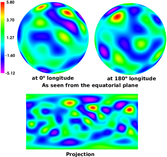
Figure 1: Arbitrary initial vorticity field computed from the spherical harmonic modes. The bottom panel shows the spherical surface projected using the standard orthographic projection.

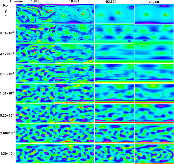
Figure 2: Time evolution of vorticity field as a function of Ro, showing diminishing enstrophy cascade and zonalization of vortical structures with decreasing Ro.

In order to quantify the effect of rotation, vorticity power spectra, spectral distribution of vorticity power, vorticity probability density, probability density of aspect ratio (ratio of major to minor axis length of vortical structures) and the cosine of the angle between the major axis and the azimuthal direction (a measure of orientation of the vortical structures) are determined. These quantifications are discussed subsequently.

II.2 Vorticity power spectra

Spherical harmonics satisfying the following orthogonality relation (Wieczorek and Meschede, 2018)

$$\int_{\Omega}Y_{lm}\left(\theta,\phi\right)Y_{l^{\prime}m^{\prime}}\left(\theta,\phi\right)\mathrm{d}\Omega=4\pi\delta_{ll^{\prime}}\delta_{mm^{\prime}},$$ (2)

where $\Omega$ is the surface area of the sphere, and $\delta_{ij}$ is the Kronecker delta function. With this, the spherical harmonic expansion coefficients are expressed as

$$\omega_{lm}=\frac{1}{4\pi}\int_{\Omega}\omega\left(\theta,\phi\right)Y_{lm}\left(\theta,\phi\right)\mathrm{d}\Omega.$$ (3)

The total vorticity power in the physical and spectral domains is related as

$$\frac{1}{4\pi}\int_{\Omega}\omega^{2}\left(\theta,\phi\right)\mathrm{d}\Omega=\sum_{l=0}^{\infty}\sum_{m=-l}^{l}\omega_{lm}^{2}=\sum_{l=0}^{\infty}S_{ff}\left(l\right),$$ (4)

where $S_{ff}\left(l\right)$ is the power spectrum of vorticity. We use Eq. (4) to compute the vorticity power spectrum $S_{ff}\left(l\right)$.

Figure 3 shows vorticity power spectra for three time instants and for different rotation rates. The initial (at t = 0) vorticity power is confined to a wavenumber range of $l=4-10$. This power cascades to the larger waver numbers as the flow evolves with time. As the Rossby number decreases (increase in rotation rate), the slope of the vorticity power spectra increases. This implies that the forward cascade of enstrophy diminishes with decreasing Rossby number. With decreasing Ro, the proportion of the spectral power contained in the wave numbers $l=4-10$ increases, even at a late time t = 92.304, further supporting the observation that the enstrophy cascade diminishes with decreasing Ro. However, there is still significant power contained in the larger wave numbers, even at a very small Ro = $1.30\times 10^{-3}$, showing that the forward enstrophy cascade is not suppressed/arrested completely which is somewhat contrary to the previously held notions of the enstrophy cascade (Rhines, 1975; Yoden and Yamada, 1993; Huang, Galperin, and Sukoriansky, 2001).

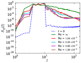
(a)

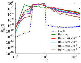
(b)

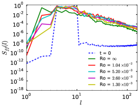
(c)

Figure 3: Vorticity power spectra as a function of wavenumber for varying Ro, depicting diminishing enstrophy cascade with decreasing Ro. Time instants shown are (a) $t=1.846$, (b) $t=18.461$, (c) $t=92.304$.

II.3 Spectral distribution of vorticity power

It is interesting to examine the effect of rotation on the distribution of the vorticity power in spectral space (i.e. using the $m-l$ space of spherical harmonics). The results are plotted in figure 4 where the spectral distribution is shown using right angle triangles: the vertical (resp. horizontal) edge of each triangle is the total wavenumber $l$ (azimuthal wave number $m$, resp.). In figure 4(a) we plot the initial vorticity power, comprising of the total modes $l=4-10$ and all of the initial zonal modes $m=4-10$, and is isotropic with respect to the zonal modes. The vorticity power cascades to smaller scales (larger $l$) as the flow evolves with time. At later times, for the non-rotating case ($\mathrm{Ro}=\infty$), the vorticity power still remain nearly uniformly distributed over all of the comprising zonal modes, and isotropic with respect to the zonal modes. With the Rossby number decreasing from infinity to $2.08\times 10^{-3}$, the vorticity power distribution tends to become concentrated in the smaller zonal modes and the distribution of the vorticity power becomes anisotropic with respect to the zonal modes. This represents the zonalization of the vortical structures and transition to Rossby wave like motions from turbulent flow with decreasing Ro. With further decrease in Ro, however, all of the comprising zonal modes tend to become equally significant, i.e., the vorticity power returns to isotropy in the zonal modes, and this is more clearly observable at late times. Thus, the zonalization of the vortical structures with decreasing Ro is non monotonic for the present case.

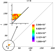
(a)

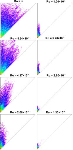
(b)

Figure 4:

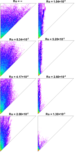
(c)

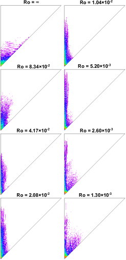
(d)

Figure 4: Vorticity power distribution in spectral space ($l,m$) for different Ro, showing diminishing enstrophy cascade with decreasing Ro and zonalization of the power. Time instants shown are (a) $t=0$, (b) $t=1.846$, (c) $t=18.461$, (d) $t=92.304$

Table 2 shows the Rhines scales (Rhines, 1975) for the present case. We choose the reference latitude to be 45° for the computation of $\beta$ here. For Ro$\leq 1.04\times 10^{-2}$, the wavenumbers ($l=4-10$) comprising the initial vorticity field are smaller than the Rhines scale (as a wavenumber, $k_{\beta}$), i.e., the scales comprising the initial vorticity field are larger than the Rhines scale (as a length scale, 1/$k_{\beta}$). Hence, according to the Rhines theory (Rhines, 1975), for the present case for Ro$\leq 1.04\times 10^{-2}$, the eddies in the initial vorticity field should not merge and initiate the inverse energy cascade (and therefore the forward enstrophy cascade) because the initial scales are already larger than the Rhines scale. However, the spectral analysis (see figures 3, 4) does show forward enstrophy cascade even for Ro$\leq 1.04\times 10^{-2}$, indicating that the cascade does not cease completely at the Rhines scale.

Ro	$k_{\beta}$		Ro	$k_{\beta}$
8.34$\times 10^{-2}$	3.878		5.20$\times 10^{-3}$	15.514
4.17$\times 10^{-2}$	5.485		2.60$\times 10^{-3}$	21.940
2.08$\times 10^{-2}$	7.757		1.30$\times 10^{-3}$	31.027
1.04$\times 10^{-2}$	10.970

Table 2: Rhines scale for case A

II.4 Vorticity probability density

The vorticity probability density/vorticity measure is defined as the area occupied by each vorticity level and expressed as

$$p\left(\omega\right)=\frac{\textrm{the area occupied by vorticity in the range $\left[\omega+\Delta\omega\right]$}}{4\pi\Delta\omega}.$$ (5)

The conservation of all Casimirs/inviscid invariants is equivalent to the conservation of $p\left(\omega\right)$ $\left(p\left(\omega+f\right)\right)$ for the non-rotating (for the rotating) inviscid flow. However, there is a lack of conservation in simulations at finite resolution because of the inevitable cascade of vorticity to small scales (Dritschel, Qi, and Marston, 2015). Here, we investigate the probability density of vorticity in the same spirit as Dritschel et al. (Dritschel, Qi, and Marston, 2015). Figure 5 shows the vorticity probability density for different Rossby numbers at $t=1.846,\,18.461$ and $92.304$. The initial (at $t=0)$ vorticity probability density is broadly distributed between $\omega_{min}=-5.1187$ and $\omega_{max}=5.7996$. For the non-rotating case, $p\left(\omega\right)$ narrows and diminishes everywhere except for values of $\omega$ near zero at late times. However, for the rotating cases, the distribution of $p\left(\omega\right)$ remains broad even at late times, and smaller the Rossby number, broader is the distribution of $p\left(\omega\right)$ at late times. This shows that as the Rossby number decreases, the forward cascade of vorticity to smaller scales decreases, consistent with the inferences made from the vorticity and power spectra plots.

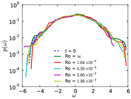
(a)

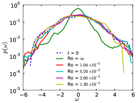
(b)

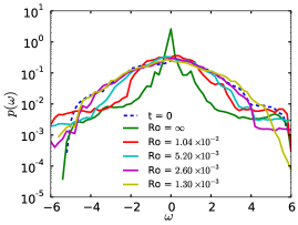
(c)

Figure 5: Vorticity probability density as a function of time and Ro. The distribution of probability density becomes broader with decreasing Ro. (a) $t=1.846$, (b) $t=18.461$, (c) $t=92.304$.

II.5 Aspect ratio and orientation of the vortical structures

We identify individual vortical structures using an algorithm (see appendix C). We determine the centroid of each individual structure from the computation of first moment of area. Hence, we have

$$\bar{\theta}_{i}=\frac{\int_{\Omega}\theta_{i}\left|\omega\right|\textrm{d}\Omega}{\int_{\Omega}\left|\omega\right|\textrm{d}\Omega}=\frac{\sum_{n=1}^{N}\left(\theta_{i}\right)_{n}\left|\omega\right|_{n}\left(\Delta\Omega\right)_{n}}{\sum_{n=1}^{N}\left|\omega\right|_{n}\left(\Delta\Omega\right)_{n}};i=1,2.$$ (6)

Here, $\theta_{1}$ and $\theta_{2}$ are the coordinates longitude and latitude respectively, and the overbar stands for the centroid coordinates, $\left|\omega\right|$ is the vorticity magnitude, $\Omega$ is the total surface area of the sphere, $\Delta\Omega$ is the dual area surrounding a primal node, and $N$ is the total number of primal nodes. We approximate each individual structure by an ellipse, and determine the major and minor axes from the computation of the second moment of area as follows. The expression of second moment of area is as follows.

$$\mu_{ij}=\frac{\int_{\Omega}\left(\theta_{i}-\bar{\theta}_{i}\right)\left(\theta_{j}-\bar{\theta}_{j}\right)\left|\omega\right|\textrm{d}\Omega}{\int_{\Omega}\left|\omega\right|\textrm{d}\Omega}$$

$$=\frac{\sum_{n=1}^{N}\left[\left(\theta_{i}\right)_{n}-\bar{\theta}_{i}\right]\left[\left(\theta_{j}\right)_{n}-\bar{\theta}_{j}\right]\left|\omega\right|_{n}\left(\Delta\Omega\right)_{n}}{\sum_{n=1}^{N}\left|\omega\right|_{n}\left(\Delta\Omega\right)_{n}};i=1,2,j=1,2.$$ (7)

Then, we compute a covariant matrix as

$$M=\left[\begin{array}[]{cc}\mu_{11}&\mu_{12}\\ \mu_{21}&\mu_{22}\end{array}\right].$$ (8)

Now, we determine the lengths of the major and minor axes of the vortical structure from the larger ($\lambda_{larger}$) and smaller ($\lambda_{smaller}$) eigenvalues of the covariant matrix, respectively. The aspect ratio, a measure of the elongation, of the vortical structure is computed as the ratio of the major axis length to the minor axis length. The orientation of the vortical structure is determined from the angle ($\alpha$, see the schematic in figure 6) between the major axis and the azimuthal direction. We determine this angle from the dot product of the eigenvector corresponding to the larger eigenvalue with the basis vector in the azimuthal direction. A representative plot showing individual structures, the major and minor axes of these structures, and the definition of the angle $\alpha$ is given in figure 6. We compute the probability density of the aspect ratio or $\cos\alpha$ as

$$p\left(f\right)=\frac{\textrm{The number of $f$ values in the range $\left[f+\Delta f\right]$}}{\textrm{Total number of $f$ values $\times$}\Delta f}.$$ (9)

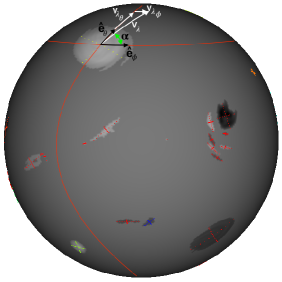
Figure 6: A representative plot showing individual vortical structures, major and minor axes, and the definition of angle $\alpha$.

Here, the function $f$ represents the aspect ratio or $\cos\alpha$ distribution. Figure 7 shows the probability density of the aspect ratio of the vortical structures as a function of Ro at late times (over the turnover time from 69.228 - 115.379). Here, the structures with aspect ratio > 20 are excluded for the sake of clarity. The lower limit of the aspect ratio (= 1) represents circular structures, and the higher values represent the elongated structures. For the non-rotating case (Ro$=\infty$), the peak in the value of probability density at aspect ratio $\approx 1$ corresponds to the presence of quadrupolar vorticity field. The decreasing probability density at larger aspect ratios corresponds to the presence of small scale vortices due to the forward enstrophy cascade. With the Rossby number decreasing from infinity to $2.08\times 10^{-2}$, the probability density peak moves away from aspect ratio $\approx 1$, showing that the vortical structures tend to elongate with decreasing Ro. In fact, these elongated structures tend to be zonal (see figure 8). With further decrease in Ro, the probability density peak tends back to move towards aspect ratio $\approx 1$. This shows that the vortical structures tend back to become circular and non-zonal (see figure 8) with further decrease in Ro. This is consistent with the aforementioned claim that the zonalization of the vortical structure is non-monotonic with decreasing Ro (for the present case).

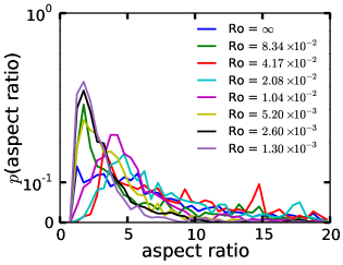
Figure 7: Probability density function of the aspect ratio of individual vortices as a function of Ro over the turnover time from 69.228 - 115.379.

Similarly, figure 8 shows the probability density of the orientation of the vortical structures (that of the cosine of the angle between the major axis and the azimuthal direction) as a function of Ro at late times (over the turnover time from 69.228 - 115.379). The upper limit $\cos\alpha=1$ represents the structures aligned in the zonal direction, and the lower values represent the non-zonal structures. For the non-rotating case (Ro$=\infty$), the relatively higher values of $p\left(\cos\alpha\right)$ at larger $\cos\alpha$ values correspond to the presence of small scale vortices due to the forward enstrophy cascade. For the rotating cases, with Ro decreasing up to $2.08\times 10^{-2}$ from infinity, $p\left(\cos\alpha\right)$ tends to increase at $\cos\alpha\approx 1$, and to vanish at smaller values of $\cos\alpha$. This indicates the zonalization of the structures with decreasing Ro. Moreover, these zonal structures have larger aspect ratio / are elongated (see figure 7). With further decrease in Ro, $p\left(\cos\alpha\right)$ tends to decrease at $\cos\alpha\approx 1$, and to augment at smaller values of $\cos\alpha$. Thus, the structures tend to become non-zonal and circular (see figure 7, the aspect ratio of these structures tend to be smaller) with further decrease in Ro. This further confirms the aforementioned claim of non-monotonic nature of the zonalization of the vortical structure with decreasing Ro (for the present case).

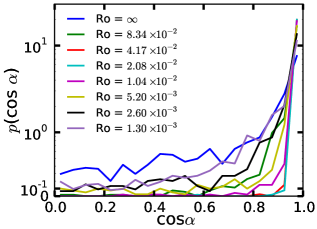
Figure 8: Probability density function of the cosine of the angle between the major axis and the azimuthal direction as a function of Ro over the turnover time from 69.228 - 115.379.

II.6 Effect of wavenumber rage constituting the (arbitrary) initial vorticity field

We consider two different arbitrary initial vorticity fields comprising of wavenumbers $l=4-10$ (test cases B, and C), and three arbitrary initial vorticity fields comprising of wavenumbers $l=4-20$, $4-40$ and $4-80$ (test cases D, E, and F). We investigate the effect of these initial conditions on the evolution of the vorticity field. The results are presented in the following sub-sections.

II.6.1 Influence of initial vorticity distribution

So far we have examined the details of vorticity evolution for case A wherein the initial vorticity was confined to the wavenumber range $l=4-10$. Figure 9 shows the evolution of the vorticity field for different initial wavenumber distributions. For each distribution we ensure that the total kinetic energy is approximately constant. Although, the initial wavenumber range for the cases B and C is the same (also, it is the same for case A), the initial amplitudes are different for these cases. For the initial vorticity field comprising of intermediate wavenumbers ($l=4-10$, test cases B, and C), at a later time, the emerging vortices from the merger of smaller scales (due to inverse cascade) tend to be zonal due to the rotation. However, the zonalization is non-monotonic with decreasing Ro. Whereas, for the initial vorticity field comprising of intermediate to large wavenumbers ($l=4-20$, $l=4-40$, and $l=4-80$; test cases D, E, and F), the zonalization tends to be monotonic with decreasing Ro. Moreover, the enstrophy cascade diminishes but does not completely cease with decreasing Ro even for the initial vorticity spectrum comprising of the scales larger than the Rhines scale. This diminishing effect tends to be weaker from test case B to F. As we move from the test case B to F, the range of scales smaller than the Rhines scale present in the initial vorticity field increases. Therefore, the cascade becomes stronger from test case B to F, and therefore the effect of rotation becomes weaker from B to F. Moreover, the scales formed from the merger of smaller scales during the inverse cascade tend to be zonal. Hence, the stronger cascade from B to F is a probable cause for the zonalization to become non-monotonic to monotonic.

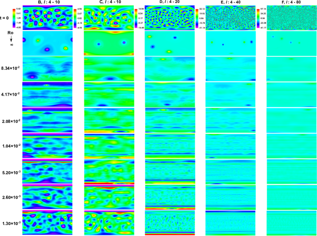
Figure 9: Vorticity distribution showing the effect of wavenumber rage comprising the (arbitrary) initial vorticity field.

II.6.2 Spectral distribution of vorticity power

Figure 10 shows the distribution of vorticity power in the spectral $\left(m-l\right)$ space as a function of the wavenumber range constituting the initial vorticity field (test cases B - F, see table 1) and Ro. For cases B and C, at a later time ($t\approx 18$), as Ro decreases the vorticity power tends to confine to smaller $m$, i.e., there is zonalization of the vortical structures. However, for Ro smaller than $5.20\times 10^{-3}$, the vorticity power tends also to be equally significant for larger $m$, showing non-monotonic nature of the zonalization. However, the confinement of the vorticity power to smaller $m$ with decreasing Ro tends to be monotonic for the cases D, E, and F, i.e., the zonalization tends to be monotonic with decreasing Ro for these cases.

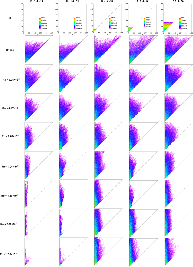
Figure 10: Spectral distribution of vorticity power showing the effect of wavenumber rage comprising the (arbitrary) initial vorticity field.

II.6.3 Probability density of orientation of vortical structures

Figure 11 shows the probability density of cosine of the angle between the major axis of the vortical structure and the azimuthal direction (that of the orientation of the vortical structures) as a function of the wavenumber range constituting the initial vorticity field and Ro. For the intermediate wavenumber range comprising the initial vorticity field (for cases B, and C), as the Ro decreases, the probability density diminishes for all of the cos$\alpha$ values except near one up to Ro of about $5.20\times 10^{-3}$. This shows the zonalization of the vortical structures. With further reduction in Ro, the probability density for cos$\alpha$ values smaller than one tends back to augment, showing nonmonotonic nature of the zonalization with decreasing Ro. However, for the initial vorticity field comprising of intermediate to large wavenumbers (for cases D, E, and F), the diminishing of the probability density for all of the cos$\alpha$ values except near unity is almost monotonic with decreasing Ro (there is insignificant augmentation of probability density values at very low Ro), revealing monotonic zonalization.

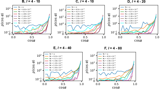
Figure 11: Probability density of cos$\alpha$ showing the effect of wavenumber rage comprising the (arbitrary) initial vorticity field.

III Conclusions

The present study examines the effect of rotation on the vorticity dynamics on a unit sphere using discrete exterior calculus. In addition to examining the effect of rotation, we also investigate different initial spectra constituting the initial vorticity field and the differences in the late time evolution of the vorticity field. The visualization of the evolving vorticity field, reveals diminishing of the forward enstrophy cascade and the non-monotonic nature of the zonalization of the vortical structures for the initial vorticity field comprising of intermediate-wavenumbers. On the other hand, the zonalization is monotonic for the initial vorticity field comprising of intermediate -to- large wavenumbers. We analyze the vorticity field on the sphere by computing the vorticity power spectrum, distribution of spectral power, vorticity probability density, probability density of aspect ratio and that of the orientation of the vortical structures. The analyses further confirms the phenomenon of zonalization although we note the tendency to zonalization reverses for high rotation rates where the initial vorticity is confined to a wavenumber range $l=4-10$. Moreover, we observe a forward cascade of enstrophy for the cases with initial vorticity field comprising of larger scales than the Rhines scale. Thus, while the forward enstrophy cascade diminishes with decreasing Rossby number, the cascade does not cease completely. The cases with initial vorticity field comprising of the scales much smaller (larger wavenumbers) than the Rhines scale have a higher potential for the cascade, and therefore, the diminishing effect of rotation is weaker for these cases. Moreover, the scales emerging from the merger of smaller scales during the inverse cascade tend to be zonal. Hence, the zonalization tend to be monotonic for these cases as the diminishing effect of rotation is weaker. Our investigation suggests that in addition to the dependence of the Rhines scale on $\beta$ and RMS velocity, the dependence on the spectrum constituting the initial vorticity field should be included in order for it to represent the scale arresting the cascade more effectively.

Appendix A Physical Setup and Numerical Procedure

We consider evolving flow on a unit sphere, and the computational domain consists of a spherical surface of unit radius. We use the DEC procedure of Jagad et al.Jagad et al. (2021). A brief description of the procedure is as follows. The governing equations consist of Euler equations in a rotating frame of reference. For an inviscid incompressible flow of a homogeneous fluid with unit density, on a compact smooth Riemannian surface, the vector calculus notation of Euler equations in a rotating frame of reference are as follows

$$\frac{\partial\mathbf{v}}{\partial t}+\nabla_{\mathbf{v}}\mathbf{v}+\textrm{grad}_{S}p+f\hat{k}\times\mathbf{v}=0,$$ (10)

$$\textrm{div}_{S}\mathbf{v}=0,$$ (11)

where $\mathbf{v}$ is the tangential surface velocity, $p$ is the effective surface pressure (which includes the centrifugal force), $\nabla_{\mathbf{v}}$ is the covariant directional derivative, $\textrm{grad}_{S}$ is the surface gradient, $\textrm{div}_{S}$ is the surface divergence, $f$ is the Coriolis parameter, and $\hat{k}$ is the unit vector in the direction of the axis of rotation. For a flavour on scaling, the nondimensional form of equation (10) can be written as

$$\frac{\partial\mathbf{v}^{\ast}}{\partial t^{\ast}}+\nabla_{\mathbf{v}}^{\ast}\mathbf{v}^{\ast}+\textrm{grad}_{S}^{\ast}p^{\ast}+\frac{1}{\mathrm{Ro}}\hat{k}\times\mathbf{v}^{\ast}=0.$$ (12)

Here, advective time scale is used as the characteristic time scale. Equation (12) shows that for low Ro (high rotation rate), the Coriolis force term dominates over the nonlinear advection term. The 2D coordinate invariant form of equations (10) - (11) read

$$\frac{\partial\mathbf{u}}{\partial t}+\ast\left(\mathbf{u}\wedge\ast d\mathbf{u}\right)+dp^{d}+\ast\left(\mathbf{u}\wedge\ast f_{2}\right)=0.$$ (13)

$$\ast\textrm{d}\ast u=0.$$ (14)

Here, $u$ is the 1-form velocity, d is the exterior derivative, $\ast$ is the Hodge star operator, $\wedge$ is the wedge product operator, $p^{d}=p+\frac{1}{2}\left(u\left(\mathbf{v}\right)\right)$ is the effective dynamic pressure 0-form, and the Coriolis force $f\hat{k}\times\mathbf{v}=\ast\left(u\wedge\ast f_{2}\right)$, where $f_{2}$ is the 2-form corresponding to $f$. We consider domain discretization with a primal simplicial mesh and there is a corresponding dual mesh (we consider the circumcentric dual). The discrete forms are now the integral quantities on the mesh elements. The discrete exterior calculus expressions of the governing equation are then expressed as

$$\left[\left(-\frac{1}{\Delta t}\right)I-\frac{1}{2}\left(W_{V}\right)^{n+1}\ast_{0}^{-1}\left[-d_{0}^{T}\right]\ast_{1}\right]\left(U^{*}\right)^{n+1}+\ast_{1}^{-1}d_{1}^{T}\left(P^{d}\right)^{n+1}=F,$$ (15)

with

$$F=\left(-\frac{1}{\Delta t}\right)\left(U^{*}\right)^{n}+\frac{1}{2}\left(W_{V}\right)^{n+1}\ast_{0}^{-1}d_{b}\left(V\right)^{n+1}+\frac{1}{2}\left(W_{V}\right)^{n}\ast_{0}^{-1}\left(\left[-d_{0}^{T}\right]\ast_{1}\left(U^{*}\right)^{n}+d_{b}\left(V\right)^{n}\right)$$

$$+\frac{1}{2}\left[\left(W_{V}\right)^{n+1}+\left(W_{V}\right)^{n}\right]\ast_{0}^{-1}f_{dual2},$$ (16)

$$\left[d_{1}\right]\left(U^{*}\right)^{n+1}+\left[0\right]\left(P^{d}\right)^{n+1}=0,$$ (17)

where $U^{\ast}$ is the vector containing mass flux primal 1-form for all mesh primal edges, $V$ is the vector containing the discrete primal velocity 1-forms for all mesh primal edges, and $P^{d}$ is the vector containing discrete dynamic pressure 0-forms for all mesh dual vertices, $\Delta t$ is the discrete time interval, $d_{0}$, $\left[-d_{0}^{T}\right]$, $d_{1}^{T}$ are the discrete exterior derivative operators, $\ast_{0}^{-1}$, $\ast_{1}$, $\ast_{1}^{-1}$ are discrete Hodge star operators. The dual-2 form $f_{dual2}$ corresponds to the Coriolis parameter $f=2\Omega\cos\theta$, where $\Omega$ is the rate of rotation of the sphere, and $\theta$ is the colatitude. The present discretization uses the energy-preserving time integration (Mullen et al., 2009). We employ a biharmonic viscosity as a means to filter and dissipate very high wavenumber content. The spherical surface domain is discretized using about 0.25M nearly uniform triangles and about 0.13M vertices for all simulation cases considered presently.The set of nonlinear equations represented by equations (15) - (17) are solved using Picard’s iterative method for the mass flux 1-form and dynamic pressure degrees of freedom. The convergence criterion of $L_{2}$ norm on the residual $\left\|R\right\|_{2}\leq 10^{-8}$ is used.

Appendix B Verification of the Numerical Procedure

We investigate the time evolution of vorticity field from the same random initial vorticity field as used in Dritschel et al.Dritschel, Qi, and Marston (2015) (see figure 12a), and compare our results with theirs and that of Modin & VivianiModin and Viviani (2020). Our simulations are based on DEC, whereas Dritschel et al.Dritschel, Qi, and Marston (2015) used Geodesic Grid Method (GGM), which is approximately second-order accurate, and Combined Lagrangian Advection Method (CLAM), which is approximately sixteen times finer in each direction than the GGM method for a given mesh, for their simulations. Modin & VivianiModin and Viviani (2020) used a casimir preserving scheme. The GGM, CLAM, and DEC methods employed, whereas the casimir preserving scheme did not employ the hyperviscosity in the momentum equation. The vorticity evolution at early times (see figure 12b) is nearly indistinguishable in all simulations (see Modian & VivianiModin and Viviani (2020) for their results). By $t=18.461$ ($t$ is the eddy turnover time), the vorticity filaments thin exponentially and the vorticity gradients grow exponentially. The numerical simulations at finite resolution cannot follow this behavior (Dritschel, Qi, and Marston, 2015). Although, the vorticity field is not identical, it is qualitatively similar in all simulations (see figure 12c). Similarly, at $t=184.61$ the vorticity field is qualitatively similar in all simulations (see figure 12d). The vorticity power spectra (see equation (4) and figure 13), and vorticity probability density (see equation (5) and figure 14) are also in agreement with that in Dritschel et al.Dritschel, Qi, and Marston (2015). Figure 15 shows the inviscid invariants as a function of time. The total circulation $\Gamma$ is conserved to the machine precision. We employ a biharmonic viscosity as a means to filter and dissipate very high wavenumber content, and less than 0.5% of the total kinetic energy dissipates by $t=500$. About 0.66% of the total enstrophy $Z$ is lost by $t=1.846$. By $t=18.461$, about 64% of the total enstrophy dissipates. At $t=184.61$ the enstrophy decays to about 20% of its initial value. A similar amount of dissipation has also been reported in Dritschel et al.Dritschel, Qi, and Marston (2015). Further verification and validation of the DEC method is discussed in the referencesMohamed, Hirani, and Samtaney, 2016; Jagad et al., 2021; Jagad, Mohamed, and Samtaney, 2020.

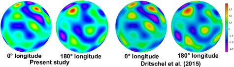
(a)

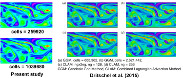
(b)

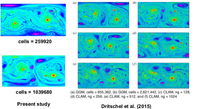
(c)

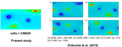
(d)

Figure 12: Evolution of the vorticity field from an initial arbitrary vorticity field for the verification case. (a) $t=0$, (b) $t=1.846$, (c) $t=18.461$, (d) $t=184.61$. The right panel figures: Dritschel, D. G., Qi, W., & Marston, J. B., On the late-time behaviour of a bounded, inviscid two-dimensional flow, Journal of Fluid Mechanics, 783, page 6-9, reproduced with permission.

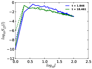
Figure 13: Vorticity power spectra. The solid line are the DEC results (present study), and the dashed lines are the CLAM results with $n_{g}=1024$ (Dritschel, Qi, and Marston, 2015).

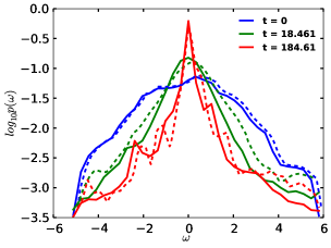
Figure 14: Vorticity probability density. The solid line are the DEC results (present study), and the dashed lines are the CLAM results with $n_{g}=1024$ (Dritschel, Qi, and Marston, 2015).

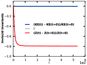
Figure 15: Inviscid invariants as a function of time. The circulation is preserved to the machine precision, the total kinetic energy and enstrophy decay by 0.5% and 80%, respectively, due to the presence of hyperviscosity term in the momentum equation.

Appendix C Segmentation Algorithm for Identifying Individual Vortical Structures

The pseudo-code for the algorithm to identify individual vortices are as follows.

• Read and store the connecting / neighboring nodes to each node in the mesh.

• The vorticity magnitude at each node is known from the solution. Chose a suitable threshold value for the vorticity magnitude. Flag the nodes greater than or equal to threshold value as 1 and include them in a list. Flag the remaining nodes as 0.

• Scroll / loop through the list of nodes with flag = 1:

  • If the flag of the node is 1 include this node in the node list for a vortical structure. Set the nfound count to 1.

  • While nfound is greater than 0:

    • Call the function Fill(node list).

    • Update the node list from the list of connecting / neighboring nodes received from the function Fill. Also, updated nfound corresponding to the list of connecting / neighboring nodes is received from the function Fill.

Fill function

• Scroll through the nodes in the node list (supplied via a function argument):

  • Set the flag of the node to 0.

  • Set the nfound count to 0.

  • Scroll through the connecting / neighboring nodes to the node being scrolled in the outer loop. If the flag of the neighboring node is 1, include this node in the list of connecting nodes and increase the nfound count by 1, flag this node as 0.

  • Return the list of connecting nodes and nfound to the calling function.

References

- Lorenz (1969) E. N. Lorenz, “The predictability of a flow which possesses many scales of motion,” Tellus 21, 289–307 (1969).
- Leith (1971) C. E. Leith, “Atmospheric predictability and two-dimensional turbulence,” Journal of Atmospheric Sciences 28, 145–161 (1971).
- Leith and Kraichnan (1972) C. E. Leith and R. H. Kraichnan, “Predictability of turbulent flows,” Journal of the Atmospheric Sciences 29, 1041–1058 (1972).
- Kraichnan (1967) R. H. Kraichnan, “Inertial ranges in two-dimensional turbulence,” The Physics of Fluids 10, 1417–1423 (1967).
- Kraichnan and Montgomery (1980) R. H. Kraichnan and D. Montgomery, “Two-dimensional turbulence,” Reports on Progress in Physics 43, 547–619 (1980).
- Leith (1968) C. E. Leith, “Diffusion approximation for two-dimensional turbulence,” The Physics of Fluids 11, 671–672 (1968).
- Lilly (1969) D. K. Lilly, “Numerical simulation of two-dimensional turbulence,” The Physics of Fluids 12, 240 – 249 (1969).
- Batchelor (1969) G. K. Batchelor, “Computation of the energy spectrum in homogeneous two-dimensional turbulence,” The Physics of Fluids 12, 233 – 239 (1969).
- Newell (1969) A. C. Newell, “Rossby wave packet interactions,” Journal of Fluid Mechanics 35, 255–271 (1969).
- Huang and Robinson (1998) H.-P. Huang and W. A. Robinson, “Two-dimensional turbulence and persistent zonal jets in a global barotropic model,” Journal of the Atmospheric Sciences 55, 611–632 (1998).
- Rhines (1975) P. B. Rhines, “Waves and turbulence on a beta-plane,” Journal of Fluid Mechanics 69, 417–443 (1975).
- Holloway and Hendershott (1977) G. Holloway and M. C. Hendershott, “Stochastic closure for nonlinear Rossby waves,” Journal of Fluid Mechanics 82, 747–765 (1977).
- Shepherd (1987) T. G. Shepherd, “Rossby waves and two-dimensional turbulence in a large-scale zonal jet,” Journal of Fluid Mechanics 183, 467–509 (1987).
- Shepherd (1987) T. G. Shepherd, “A spectral view of nonlinear fluxes and stationary-transient interaction in the atmosphere,” Journal of Atmospheric Sciences 44, 1166–1179 (1987).
- Yamada and Yoneda (2013) M. Yamada and T. Yoneda, “Resonant interaction of Rossby waves in two-dimensional flow on a - plane,” Physica D: Nonlinear Phenomena 245, 1 – 7 (2013).
- Vallis and Maltrud (1993) G. K. Vallis and M. E. Maltrud, “Generation of mean flows and jets on a beta plane and over topography,” Journal of Physical Oceanography 23, 1346–1362 (1993).
- Maltrud and Vallis (1991) M. E. Maltrud and G. K. Vallis, “Energy spectra and coherent structures in forced two-dimensional and beta-plane turbulence,” Journal of Fluid Mechanics 228, 321–342 (1991).
- Huang, Galperin, and Sukoriansky (2001) H.-P. Huang, B. Galperin, and S. Sukoriansky, “Anisotropic spectra in two-dimensional turbulence on the surface of a rotating sphere,” Physics of Fluids 13, 225–240 (2001).
- Chekhlov et al. (1996) A. Chekhlov, S. A. Orszag, S. Sukoriansky, B. Galperin, and I. Staroselsky, “The effect of small-scale forcing on large-scale structures in two-dimensional flows,” Physica D: Nonlinear Phenomena 98, 321 – 334 (1996).
- Basdevant et al. (1981) C. Basdevant, B. Legras, R. Sadourny, and M. Béland, “A study of barotropic model flows: Intermittency, waves and predictability,” Journal of the Atmospheric Sciences 38, 2305–2326 (1981).
- Legras (1980) B. Legras, “Turbulent phase shift of Rossby waves,” Geophysical & Astrophysical Fluid Dynamics 15, 253–281 (1980).
- Bartello and Holloway (1991) P. Bartello and G. Holloway, “Passive scalar transport in -plane turbulence,” Journal of Fluid Mechanics 223, 521–536 (1991).
- Sukoriansky, Galperin, and Staroselsky (1994) S. Sukoriansky, B. Galperin, and I. Staroselsky, “Large-scale dynamics of two-dimensional turbulence with rossby waves,” in Progress in Turbulence Research, Vol. 162 (Aiaa, 1994) pp. 108–120.
- Panetta (1993) R. L. Panetta, “Zonal jets in wide baroclinically unstable regions: Persistence and scale selection,” Journal of the Atmospheric Sciences 50, 2073–2106 (1993).
- Marcus and Lee (1994) P. S. Marcus and C. Lee, “Jupiter’s great red spot and zonal winds as a self-consistent, one-layer, quasigeostrophic flow,” Chaos: An Interdisciplinary Journal of Nonlinear Science 4, 269–286 (1994).
- Rhines (1994) P. B. Rhines, “Jets,” Chaos: An Interdisciplinary Journal of Nonlinear Science 4, 313–339 (1994).
- Sukoriansky, Dikovskaya, and Galperin (2007) S. Sukoriansky, N. Dikovskaya, and B. Galperin, “On the arrest of inverse energy cascade and the Rhines scale,” Journal of the Atmospheric Sciences 64, 3312–3327 (2007).
- Yoden and Yamada (1993) S. Yoden and M. Yamada, “A numerical experiment on two-dimensional decaying turbulence on a rotating sphere,” Journal of the Atmospheric Sciences 50, 631–644 (1993).
- Cho and Polvani (1996) J. Y.-K. Cho and L. M. Polvani, “The emergence of jets and vortices in freely evolving, shallow-water turbulence on a sphere,” Physics of Fluids 8, 1531–1552 (1996).
- Yoden et al. (1999) S. Yoden, K. Ishioka, Y.-Y. Hayashi, and M. Yamada, “A further experiment on two-dimensional decaying turbulence on a rotating sphere,” Nuovo Cimento della Societa Italiana di Fisica C 22, 803–812 (1999).
- Hayashi et al. (2000) Y.-Y. Hayashi, K. Ishioka, M. Yamada, and S. Yoden, “Emergence of circumpolar vortex in two dimensional turbulence on a rotating sphere,” in IUTAM Symposium on Developments in Geophysical Turbulence, edited by R. M. Kerr and Y. Kimura (Springer Netherlands, Dordrecht, 2000) pp. 179–192.
- Ishioka et al. (2000) K. Ishioka, M. Yamada, Y.-Y. Hayashi, and S. Yoden, “Technical approach for the design of a high-resolution spectral model on a sphere: Application to decaying turbulence,” Nonlinear Processes in Geophysics 7, 105–110 (2000).
- Hayashi et al. (2007) Y.-Y. Hayashi, S. Nishizawa, S.-i. Takehiro, M. Yamada, K. Ishioka, and S. Yoden, “Rossby waves and jets in two-dimensional decaying turbulence on a rotating sphere,” Journal of the Atmospheric Sciences 64, 4246–4269 (2007).
- Takehiro, Yamada, and Hayashi (2007a) S. Takehiro, M. Yamada, and Y.-Y. Hayashi, “Circumpolar jets emerging in two-dimensional non-divergent decaying turbulence on a rapidly rotating sphere,” Fluid Dynamics Research 39, 209–220 (2007a).
- Takehiro, Yamada, and Hayashi (2007b) S. Takehiro, M. Yamada, and Y.-Y. Hayashi, “Energy accumulation in easterly circumpolar jets generated by two-dimensional barotropic decaying turbulence on a rapidly rotating sphere,” Journal of the Atmospheric Sciences 64, 4084–4097 (2007b).
- Yoden et al. (2003) S. Yoden, K. Ishioka, M. Yamada, and Y.-Y. Hayashi, “Pattern formation in two-dimensional turbulence on a rotating sphere,” in Statistical Theories and Computational Approaches to Turbulence, edited by Y. Kaneda and T. Gotoh (Springer Japan, Tokyo, 2003) pp. 317–326.
- Sasaki, Takehiro, and Yamada (2012) E. Sasaki, S.-i. Takehiro, and M. Yamada, “A note on the stability of inviscid zonal jet flows on a rotating sphere,” Journal of Fluid Mechanics 710, 154–165 (2012).
- Saito and Ishioka (2016) I. Saito and K. Ishioka, “On a quasi-invariant associated with the emergence of anisotropy in two-dimensional turbulence on a rotating sphere,” Journal of the Meteorological Society of Japan. Ser. II 94, 25–39 (2016).
- Obuse and Yamada (2019) K. Obuse and M. Yamada, “Three-wave resonant interactions and zonal flows in two-dimensional Rossby-Haurwitz wave turbulence on a rotating sphere,” Phys. Rev. Fluids 4, 024601 (2019).
- Farge and Sadourny (1989) M. Farge and R. Sadourny, “Wave-vortex dynamics in rotating shallow water,” Journal of Fluid Mechanics 206, 433–462 (1989).
- Yuan and Hamilton (1994) L. Yuan and K. Hamilton, “Equilibrium dynamics in a forced-dissipative f-plane shallow-water system,” Journal of Fluid Mechanics 280, 369–394 (1994).
- Iacono, Struglia, and Ronchi (1999) R. Iacono, M. V. Struglia, and C. Ronchi, “Spontaneous formation of equatorial jets in freely decaying shallow water turbulence,” Physics of Fluids 11, 1272–1274 (1999).
- Kitamura and Ishioka (2007) Y. Kitamura and K. Ishioka, “Equatorial jets in decaying shallow-water turbulence on a rotating sphere,” Journal of the Atmospheric Sciences 64, 3340–3353 (2007).
- Yoden et al. (2010) S. Yoden, Y.-Y. Hayashi, K. Ishioka, Y. Kitamura, S. Nishizawa, S.-i. Takehiro, and M. Yamada, “Jet formation in decaying two-dimensional turbulence on a rotating sphere,” in IUTAM Symposium on Turbulence in the Atmosphere and Oceans, edited by D. Dritschel (Springer Netherlands, Dordrecht, 2010) pp. 253–263.
- Williams (1978) G. P. Williams, “Planetary circulations: 1. barotropic representation of Jovian and terrestrial turbulence,” Journal of the Atmospheric Sciences 35, 1399–1426 (1978).
- Nozawa and Yoden (1997a) T. Nozawa and S. Yoden, “Spectral anisotropy in forced two-dimensional turbulence on a rotating sphere,” Physics of Fluids 9, 3834–3842 (1997a).
- Nozawa and Yoden (1997b) T. Nozawa and S. Yoden, “Formation of zonal band structure in forced two-dimensional turbulence on a rotating sphere,” Physics of Fluids 9, 2081–2093 (1997b).
- McWilliams (1984) J. C. McWilliams, “The emergence of isolated, coherent vortices in turbulent flow,” AIP Conference Proceedings 106, 205–221 (1984).
- Sukoriansky, Galperin, and Dikovskaya (2002) S. Sukoriansky, B. Galperin, and N. Dikovskaya, “Universal spectrum of two-dimensional turbulence on a rotating sphere and some basic features of atmospheric circulation on giant planets,” Phys. Rev. Lett. 89, 124501 (2002).
- Scott and Polvani (2007) R. K. Scott and L. M. Polvani, “Forced-dissipative shallow-water turbulence on the sphere and the atmospheric circulation of the giant planets,” Journal of the Atmospheric Sciences 64, 3158–3176 (2007).
- Obuse, Takehiro, and Yamada (2010) K. Obuse, S.-i. Takehiro, and M. Yamada, “Long-time asymptotic states of forced two-dimensional barotropic incompressible flows on a rotating sphere,” Physics of Fluids 22, 056601 (2010).
- Galperin, Sukoriansky, and Huang (2001) B. Galperin, S. Sukoriansky, and H.-P. Huang, “Universal spectrum of zonal flows on giant planets,” Physics of Fluids 13, 1545–1548 (2001).
- Galperin et al. (2004) B. Galperin, H. Nakano, H.-P. Huang, and S. Sukoriansky, “The ubiquitous zonal jets in the atmospheres of giant planets and earth’s oceans,” Geophysical Research Letters 31 (2004).
- Galperin et al. (2006) B. Galperin, S. Sukoriansky, N. Dikovskaya, P. L. Read, Y. H. Yamazaki, and R. Wordsworth, “Anisotropic turbulence and zonal jets in rotating flows with a -effect,” Nonlinear Processes in Geophysics 13, 83–98 (2006).
- Galperin, Sukoriansky, and Dikovskaya (2008) B. Galperin, S. Sukoriansky, and N. Dikovskaya, “Zonostrophic turbulence,” Physica Scripta T132, 014034 (2008).
- Vallis (2017) G. K. Vallis, Atmospheric and Oceanic Fluid Dynamics: Fundamentals and Large-Scale Circulation, 2nd ed. (Cambridge University Press, 2017).
- Read et al. (2004) P. L. Read, Y. H. Yamazaki, S. R. Lewis, P. D. Williams, K. Miki-Yamazaki, J. Sommeria, H. Didelle, and A. Fincham, “Jupiter’s and Saturn’s convectively driven banded jets in the laboratory,” Geophysical Research Letters 31 (2004).
- Read et al. (2007) P. L. Read, Y. H. Yamazaki, S. R. Lewis, P. D. Williams, R. Wordsworth, K. Miki-Yamazaki, J. Sommeria, and H. Didelle, “Dynamics of convectively driven banded jets in the laboratory,” Journal of the Atmospheric Sciences 64, 4031–4052 (2007).
- Sukoriansky, Dikovskaya, and Galperin (2008) S. Sukoriansky, N. Dikovskaya, and B. Galperin, “Nonlinear waves in zonostrophic turbulence,” Phys. Rev. Lett. 101, 178501 (2008).
- Flanders (1963) H. Flanders, Mathematics in Science and Engineering, 1st ed., Vol. 11 (Elsevier, 1963).
- Abraham, Marsden, and Ratiu (2012) R. Abraham, J. E. Marsden, and T. Ratiu, Manifolds, tensor analysis, and applications, Vol. 75 (Springer Science & Business Media, 2012).
- Hirani (2003) A. N. Hirani, Discrete exterior calculus, Ph.D. thesis, California Institute of Technology (2003).
- Desbrun, Hirani, and Marsden (2003) M. Desbrun, A. N. Hirani, and J. E. Marsden, “Discrete exterior calculus for variational problems in computer vision and graphics,” in Decision and Control, 2003. Proceedings. 42nd IEEE Conference on, Vol. 5 (IEEE, 2003) pp. 4902–4907.
- Desbrun et al. (2005) M. Desbrun, A. N. Hirani, M. Leok, and J. E. Marsden, “Discrete exterior calculus,” arXiv preprint math/0508341 (2005).
- Grinspun et al. (2006) E. Grinspun, M. Desbrun, K. Polthier, P. Schröder, and A. Stern, “Discrete differential geometry: an applied introduction,” ACM Siggraph Course 7, 1–139 (2006).
- Hirani, Nakshatrala, and Chaudhry (2008) A. N. Hirani, K. B. Nakshatrala, and J. H. Chaudhry, “Numerical method for Darcy flow derived using discrete exterior calculus,” arXiv preprint arXiv:0810.3434 (2008).
- Desbrun, Kanso, and Tong (2008) M. Desbrun, E. Kanso, and Y. Tong, “Discrete differential forms for computational modeling,” in Discrete differential geometry (Springer, 2008) pp. 287–324.
- Crane et al. (2013) K. Crane, F. De Goes, M. Desbrun, and P. Schröder, “Digital geometry processing with discrete exterior calculus,” in ACM SIGGRAPH 2013 Courses (2013) pp. 1–126.
- Perot and Zusi (2014) J. B. Perot and C. J. Zusi, “Differential forms for scientists and engineers,” Journal of Computational Physics 257, 1373–1393 (2014).
- Mohamed, Hirani, and Samtaney (2016) M. S. Mohamed, A. N. Hirani, and R. Samtaney, “Discrete exterior calculus discretization of incompressible Navier–Stokes equations over surface simplicial meshes,” Journal of Computational Physics 312, 175–191 (2016).
- de Goes et al. (2016) F. de Goes, M. Desbrun, M. Meyer, and T. DeRose, “Subdivision exterior calculus for geometry processing,” ACM Transactions on Graphics (TOG) 35, 1–11 (2016).
- Jagad et al. (2021) P. Jagad, A. Abukhwejah, M. Mohamed, and R. Samtaney, “A primitive variable discrete exterior calculus discretization of incompressible Navier-Stokes equations over surface simplicial meshes,” Physics of Fluids 33, 017114 (2021).
- Dritschel, Qi, and Marston (2015) D. G. Dritschel, W. Qi, and J. Marston, “On the late-time behaviour of a bounded, inviscid two-dimensional flow,” Journal of Fluid Mechanics 783, 1–22 (2015).
- Wieczorek and Meschede (2018) M. A. Wieczorek and M. Meschede, “Shtools: Tools for working with spherical harmonics,” Geochemistry, Geophysics, Geosystems 19, 2574–2592 (2018).
- Mullen et al. (2009) P. Mullen, K. Crane, D. Pavlov, Y. Tong, and M. Desbrun, “Energy-preserving integrators for fluid animation,” ACM Trans. Graph. 28, 38 (2009).
- Modin and Viviani (2020) K. Modin and M. Viviani, “A casimir preserving scheme for long-time simulation of spherical ideal hydrodynamics,” Journal of Fluid Mechanics 884, A22 (2020).
- Jagad, Mohamed, and Samtaney (2020) P. Jagad, M. S. Mohamed, and R. Samtaney, “Investigation of flow past a cylinder embedded on curved and flat surfaces,” Phys. Rev. Fluids 5, 044701 (2020).