Metric dimensions vs. cyclomatic number of graphs with minimum degree at least two

Abstract

The vertex (resp. edge) metric dimension of a connected graph $G,$ denoted by $\mathrm{dim}(G)$ (resp. $\mathrm{edim}(G)$), is defined as the size of a smallest set $S\subseteq V(G)$ which distinguishes all pairs of vertices (resp. edges) in $G.$ Bounds $\mathrm{dim}(G)\leq L(G)+2c(G)$ and $\mathrm{edim}(G)\leq L(G)+2c(G),$ where $c(G)$ is the cyclomatic number in $G$ and $L(G)$ depends on the number of leaves in $G$, are known to hold for cacti and are conjectured to hold for general graphs. In leafless graphs it holds that $L(G)=0,$ so for such graphs the conjectured upper bound becomes $2c(G).$ In this paper, we show that the bound $2c(G)$ cannot be attained by leafless cacti, so the upper bound for such cacti decreases to $2c(G)-1$, and we characterize all extremal leafless cacti for the decreased bound. We conjecture that the decreased bound holds for all leafless graphs, i.e. graphs with minimum degree at least two. We support this conjecture by showing that it holds for all graphs with minimum degree at least three and that it is sufficient to show that it holds for all $2$-connected graphs, and we also verify the conjecture for graphs of small order.

1 Introduction

All graphs in this paper are tacitly assumed to be connected. We consider several metric dimensions in connected graphs, and all of them involve the notion of distance, so we define it here first. For a pair of vertices $u$ and $v,$ the distance $d(u,v)$ is defined as the length of the shortest path connecting vertices $u$ and $v$. For a pair consisting of a vertex $u$ and an edge $e=vw,$ the distance $d(u,e)$ is defined by $d(u,e)=\min\{d(u,v),d(u,w)\}.$ Now, let $s$ be a vertex from $G$ and $X\subseteq V(G)\cup E(G),$ we say that a pair $x$ and $x^{\prime}$ from $X$ is distinguished by $s$ if $d(s,x)\not=d(s,x^{\prime})$. We say that the set $S\subseteq V(G)$ is a metric generator of $X,$ if every pair $x,x^{\prime}\in X$ is distinguished by at least one vertex from $S.$ Especially, if $S$ is a metric generator of $X=V(G)$ (resp. $X=E(G),$ $X=V(G)\cup E(G)$) then $S$ is a vertex (resp. edge, mixed) metric generator. The cardinality of a smallest vertex (resp. edge, mixed) metric generator is the vertex (resp. edge, mixed) metric dimension of $G$ and it is denoted by $\mathrm{dim}(G)$ (resp. $\mathrm{edim}(G),$ $\mathrm{mdim}(G)$).

The concept of vertex metric dimension is chronologically the first introduced and it was studied related to the navigation systems [4] and the problem of landmarks in networks [7]. Since then this variant of metric dimension was extensively investigated from various aspects [1, 2, 8, 10]. Recently it was noted that for some graphs the smallest vertex metric generators do not distinguish all pairs of edges [6], so the notion of edge metric dimension of a graph was introduced. This variant of metric dimension, even though it is more recent, has also been quite studied [3, 9, 11, 17, 18]. Finally, as a natural next step the mixed metric dimension of a graph was introduced in [5] and later further investigated in [13, 14]. For this paper particularly relevant is the line of investigation from papers [12, 15, 16] where an upper bound on vertex and edge metric dimensions was established for unicyclic graphs and further extended to cacti. There it was also conjectured that the bound holds for connected graphs in general. In this paper we focus on cacti without leaves and show that for such graphs the bound decreases by one and we characterize which cacti without leaves attain this decreased bound.

For a vertex $v$ of a graph $G,$ the degree $\deg(v)$ is the number of vertices in $G$ adjacent to $v.$ The minimum degree in a graph $G$ is denoted by $\delta(G)$. If $\deg(v)=1,$ then we say $v$ is a leaf. We say that a set $S\subseteq V(G)$ is a vertex cut if $G-S$ is disconnected or trivial. If $S=\{v\}$ is a vertex cut, then we say $v$ is a cut vertex. The (vertex) connectivity of a graph $G,$ denoted by $\kappa(G),$ is defined as the cardinality of the smallest vertex cut in $G.$ A graph $G$ is $k$-connected if $\kappa(G)\geq k.$ Notice that $\kappa(G)\leq\delta(G)$, so $2$-connected graphs do not contain leaves. Also, polycyclic cacti obviously have $\kappa(G)=1.$ A block in a graph $G$ is any maximal $2$-connected subgraph of $G.$ A block $G_{i}$ in $G$ is non-trivial, if $G_{i}$ contains at least three vertices. We say that a block $G_{i}$ of $G$ is an end-block if $G_{i}$ contains precisely one cut vertex from $G$.

Let $P=u_{1}\ldots u_{k}$ be an induced subpath of $G$ and let $v\in V(G)$ be a vertex in $G$ of degree at least three. We say that $P$ is a thread in $G$ hanging at $v$ if the vertex $u_{1}$ is a leaf in $G$ and $u_{k}$ is adjacent to $v$. We define the number $L(G)$ by

$$L(G)=\sum_{v\in V(G),\ell(v)>1}(\ell(v)-1)$$

where $\ell(v)$ is the number of threads hanging at a vertex $v$. Notice that $\ell(v)>0$ may hold only for a vertex $v$ with degree $\geq 3$. The cyclomatic number $c(G)$ of a graph $G$ is defined by $c(G)=\left|E(G)\right|-\left|V(G)\right|+1.$ The following upper bounds on $\mathrm{dim}(G)$ and $\mathrm{edim}(G)$ are conjectured in [15], where it was also shown that the conjectured bounds hold for graphs with edge disjoint cycles (also called cactus graphs or cacti) and all extremal graphs characterized.

Conjecture 1

Let $G$ be a connected graph. Then, $\mathrm{dim}(G)\leq L(G)+2c(G).$

Conjecture 2

Let $G$ be a connected graph. Then, $\mathrm{edim}(G)\leq L(G)+2c(G).$

In this paper we further investigate these conjectures. First, we notice that the attainment of the bounds in the class of cacti depends on the presence of leaves in a graph and that the bounds cannot be attained by cacti without leaves. The natural question that arises is what is the tight upper bound for leafless cacti and does it extend to all graphs without leaves. We start the investigation of that question by characterizing all cacti for which the first smaller bound is attained, i.e. all cacti for which $\mathrm{dim}(G)=L(G)+2c(G)-1$ (resp. $\mathrm{edim}(G)=L(G)+2c(G)-1$). The direct consequence is that this upper bound is attained by some leafless cacti, and therefore it is a tight bound.

For all leafless graphs it holds that $L(G)=0,$ so the upper bound from Conjectures 1 and 2 becomes $2c(G),$ and we suspect that it cannot be attained by such graphs, just as it cannot be attained by leafless cacti. Notice that a graph $G$ being leafless is equivalent to its minimum degree being at least two. We state a formal conjecture that both metric dimensions of such graphs are bounded above by $2c(G)-1.$ As a first step towards the solution of this conjecture, we show that the upper bound $2c(G)-1$ holds for both metric dimensions of all graphs with $\delta(G)\geq 3$ and moreover the bound cannot be attained by them. This reduces the problem to the class of graphs with $\delta(G)=2.$

Notice that graphs with $\delta(G)=2$ may have $\kappa(G)=1$ and $\kappa(G)=2.$ For graphs $G$ with $\delta(G)=2$ and $\kappa(G)=1$ we further show that if the upper bound $2c(G_{i})-1$ holds for a metric dimension of every non-trivial block $G_{i}$ in $G$ distinct from a cycle, then $2c(G)-1$ is also an upper bound for the metric dimensions of $G.$ This further reduces the problem to $2$-connected graphs, i.e. it only remains to prove that the upper bound $2c(G)-1$ holds for metric dimensions of graphs with $\kappa(G)=2.$ We leave this case open.

The similar results and conjectures for the mixed metric dimension are already established in [13, 14].

2 Preliminaries

Let $G$ be a cactus graph, $C$ a cycle in $G$ and $v\in V(C).$ By $G_{v}(C)$ we denote the connected component of $G-E(C)$ which contains the vertex $v.$ A vertex $v\in V(C)$ is said to be branch-active if its degree is at least $4$ or $G_{v}(C)$ contains a vertex of degree at least $3$ distinct from $v$. Notice that in the case of $v$ being a branch-active vertex, there are two vertices (resp. two edges) in $G_{v}(C)$ on the same distance from $v,$ which implies they will not be distinguished by a set $S\subseteq V(G)$ if $G_{v}(C)$ does not contain a vertex from $S.$ We denote the number of branch-active vertices on $C$ by $b(C).$

For a cactus graph $G$ with $c$ cycles $C_{1},\ldots,C_{c}$ we introduce the notation

$$B(G)=\sum_{i=1}^{c}\max\{0,2-b(C_{i})\}.$$

We say that a cycle $C_{i}$ of a cactus graph is an end-cycle if $b(C_{i})=1.$ Notice that for every cycle $C_{i}$ of a cactus graph $G$ with $c\geq 2$ cycles, it holds that $b(C_{i})\geq 1.$ Therefore, in such a graph $B(G)\leq c$ with equality if and only if every cycle is an end-cycle.

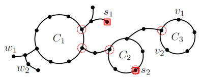
Figure 1: A cactus graph $G$ with three cycles and a set $S=\{s_{1},s_{2}\}\subseteq V(G)$ for which $S$-active vertices on each cycle are marked by a dashed circle. The set $S$ is neither biactive, nor branch-resolving. Since $S$ is not biactive on $C_{3}$, vertices $v_{1}$ and $v_{2}$ are not distinguished by $S.$ And, since $S$ is not branch-resolving due to the two $S$-free threads containing vertices $w_{1}$ and $w_{2}$ hanging at the same vertex, vertices $w_{1}$ and $w_{2}$ are not distinguished by $S.$

Let $G$ be a cactus graph, $S\subseteq V(G),$ $C$ a cycle in $G$ and $v\in V(C).$ We say that $v$ is $S$-active on $C$ if $G_{v}(C)$ contains a vertex from $S.$ By $a_{S}(C)$ we denote the number of vertices on $C$ which are $S$-active. A set $S\subseteq V(G)$ is biactive in $G$ if every cycle $C_{i}$ of $G$ contains at least two $S$-active vertices. An $S$-free thread is any thread in $G$ such that $S$ does not contain any vertex of that thread. If for a set of vertices $S\subseteq V(G)$ it holds that there are no two $S$-free threads in $G$ hanging at the same vertex, then $S$ is a branch-resolving set in $G$. Every biactive branch-resolving set will be called shortly a BBR set. It was established in [15] that every vertex (resp. edge) metric generator is a BBR set. The necessity of this condition is illustrated by Figure 1. Notice that for every smallest BBR set $S$ in a polycyclic cactus graph $G$ it holds that $\left|S\right|=L(G)+B(G).$

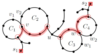
Figure 2: A cactus graph $G$ with four cycles and a BBR set $S=\{s_{1},s_{2}\}\subseteq V(G).$ On each of the four cycles the $S$-path is marked.

Throughout the paper for a given cactus graph $G$ and a BBR set $S\subseteq V(G),$ we will assume that for a cycle $C$ with $V(C)=\{v_{0},\ldots,v_{g-1}\},$ the vertices of $V(C)$ are denoted so that $v_{0}$ is $S$-active and $k=\max\{i:v_{i}$ is $S$-active$\}$ is the smallest possible. Assuming such labeling, the subpath of a cycle $C_{i}$ consisting of vertices $v_{1}v_{2}\cdots v_{k-1}v_{k}$ is called an $S$-path and denoted by $P_{i}.$ The notion of $S$-path is illustrated by Figure 2.

$\begin{array}[c]{ll}\text{a) \raisebox{-10.0pt}{\includegraphics[scale={0.8}]{Figure03.pdf}}}&\text{b) \raisebox{-10.0pt}{\includegraphics[scale={0.8}]{Figure04.pdf}}}\\ \text{c) \raisebox{-10.0pt}{\includegraphics[scale={0.8}]{Figure05.pdf}}}&\text{d) \raisebox{-10.0pt}{\includegraphics[scale={0.8}]{Figure06.pdf}}}\\ \text{e) \raisebox{-10.0pt}{\includegraphics[scale={0.8}]{Figure07.pdf}}}&\text{f) \raisebox{-10.0pt}{\includegraphics[scale={0.8}]{Figure08.pdf}}}\end{array}$

Figure 3: Each of the six graphs are unicyclic graphs with a BBR set of vertices $S=\{s_{i}\}$ marked in them. The $S$-active vertices on the cycle are marked by a dashed circle and dashed lines connect them to their antipodals, as they delimit the area on cycle where the presence of an $S$-free thread makes the configuration. The graph contains configurations: a) $\mathcal{A}$, b) $\mathcal{B}$ and $\mathcal{D},$ c) $\mathcal{C}$, d) $\mathcal{D},$ e) $\mathcal{E}$ on even cycle and $\mathcal{C}$, f) $\mathcal{E}$ on odd cycle. By $x$ and $x^{\prime}$ a pair of vertices and/or edges is denoted which is not distinguished by $S$. As illustrated by graph b) configuration $\mathcal{B}$ is at the same time also $\mathcal{D},$ but graph in d) shows that $\mathcal{D}$ does not have to be $\mathcal{B}.$ Similarly, by the graph in e) it is illustrated that $\mathcal{E}$ is at the same time $\mathcal{C},$ but the graph c) shows that the opposite does not hold, i.e. $\mathcal{C}$ is not always $\mathcal{E}$.

Let us now introduce five configurations which a cycle in a cactus graph may contain with respect to a BBR set $S.$

Definition 3

Let $G$ be a cactus graph, $C$ a cycle in $G$ of the length $g$, and $S$ a BBR set in $G$. We say that the cycle $C$ with respect to $S$ contains configurations:

$\mathcal{A}$. If $a_{S}(C)=2$, $g$ is even, and $k=g/2$;

$\mathcal{B}$. If $k\leq\left\lfloor g/2\right\rfloor-1$ and there is an $S$-free thread hanging at a vertex $v_{i}$ for some $i\in[k,\left\lfloor g/2\right\rfloor-1]\cup[\left\lceil g/2\right\rceil+k+1,g-1]\cup\{0\}$;

$\mathcal{C}$. If $a_{S}(C)=2$, $g$ is even, $k\leq g/2$ and there is an $S$-free thread of the length $\geq g/2-k$ hanging at a vertex $v_{i}$ for some $i\in[0,k]$;

$\mathcal{D}$. If $k\leq\left\lceil g/2\right\rceil-1$ and there is an $S$-free thread hanging at a vertex $v_{i}$ for some $i\in[k,\left\lceil g/2\right\rceil-1]\cup[\left\lfloor g/2\right\rfloor+k+1,g-1]\cup\{0\}$;

$\mathcal{E}$. If $a_{S}(C)=2$ and there is an $S$-free thread of the length $\geq\left\lfloor g/2\right\rfloor-k+1$ hanging at a vertex $v_{i}$ with $i\in[0,k].$ Moreover, if $g$ is even, an $S$-free thread must be hanging at the vertex $v_{j}$ with $j=g/2+k-i$.

These configurations are illustrated by Figure 3 and originally introduced in [15]. The same figure also illustrated why $S$ being a BBR set is only necessary, but not sufficient condition for $S$ to be a metric generator. Consequently, when constructing a smallest metric generator in a cactus graph $G$, one needs to start from a smallest BBR set $S$ and then consider which of the cycles in $G$ contain one of the configurations with respect to it, as for such cycles additional vertices will have to be introduced into $S.$ Since it is obviously important to consider if a cycle contains these configurations, for that purpose we introduce the following definition.

Definition 4

We say that a cycle $C_{i}$ of a cactus graph $G$ is $\mathcal{ABC}$-negative (resp. $\mathcal{ADE}$-negative), if there exists a smallest BBR set $S$ in $G$ such that $C_{i}$ does not contain any of the configurations $\mathcal{A},$ $\mathcal{B},$ and $\mathcal{C}$ (resp. $\mathcal{A},$ $\mathcal{D},$ and $\mathcal{E}$) with respect to $S.$ Otherwise, we say that $C_{i}$ is $\mathcal{ABC}$-positive (resp. $\mathcal{ADE}$-positive). The number of $\mathcal{ABC}$-positive (resp. $\mathcal{ADE}$-positive) cycles in $G$ is denoted by $c_{\mathcal{ABC}}(G)$ (resp. $c_{\mathcal{ADE}}(G)$).

It is worth noting that there exists a smallest BBR set $S$ such that every $\mathcal{ABC}$-negative (resp. $\mathcal{ADE}$-negative) does not contain the three respective configurations with respect to $S$, as it was established in [15]. There, it was also shown that the presence of the three respective configurations on any of the cycles in $G$ is an obstacle for $S$ to be a metric generator and that for each such cycle an additional vertex has to be introduced to $S$ in order for it to become a metric generator. But even that is only necessary and not sufficient condition for $S$ to be a metric generator, as there may further occur a problem when cycles share a vertex, for which we introduce the following definitions.

Definition 5

Let $G$ be a cactus graph with cycles $C_{1},\ldots,C_{c}$ and let $S$ be a BBR set in $G.$ We say that a vertex $v\in V(C_{i})$ is vertex-critical (resp. edge-critical) on $C_{i}$ with respect to $S$ if $v$ is an end-vertex of the $S$-path $P_{i}$ and $\left|P_{i}\right|\leq\left\lfloor g_{i}/2\right\rfloor-1$ (resp. $\left|P_{i}\right|\leq\left\lceil g_{i}/2\right\rceil-1$).

Notice that the notion of a vertex-critical and an edge-critical vertex differs only on odd cycles.

Definition 6

Two distinct cycles $C_{i}$ and $C_{j}$ of a cactus graph $G$ are vertex-critically incident (resp. edge-critically incident) with respect to a BBR set $S\subseteq V(G)$ if $C_{i}$ and $C_{j}$ share a vertex $v$ which is vertex-critical (resp. edge-critical) with respect to $S$ on both $C_{i}$ and $C_{j}$.

For illustration and motivation of these notions, consider the following example.

Example 7

Let $G$ be a graph and $S=\{s_{1},s_{2}\}$ a set of vertices in $G$ as shown in Figure 2. None of the four cycles in $G$ contains any of the five configurations. Vertex $v$ shared by cycles $C_{1}$ and $C_{2}$ is vertex-critical on both cycles and it is also edge-critical on both cycles. Therefore, cycles $C_{1}$ and $C_{2}$ are both vertex- and edge-critically incident. Consequently, the pair of vertices $v_{1}$ and $v_{2}$ and also the pair of edges $v_{1}v$ and $v_{2}v$ are not distinguished by $S.$

On the other hand, the vertex $w$ shared by cycles $C_{3}$ and $C_{4}$ is vertex-critical on both cycles, but edge-critical only on the cycle $C_{3}$ and not on $C_{4}.$ Therefore, cycles $C_{3}$ and $C_{4}$ are only vertex-critically incident and not edge-critically incident. A consequence of this is that the pair of vertices $w_{1}$ and $w_{2}$ on these two cycles is not distinguished by $S,$ there is no a pair of indistingushed edges (notice that $w_{1}w$ and $w_{2}w$ are distinguished by $S$).

A set $S\subseteq V(G)$ is a vertex cover if it contains a least one end-vertex of every edge in $G.$ The cardinality of a smallest vertex cover in $G$ is the vertex cover number of $G$ denoted by $\tau(G).$ Further, let $G$ be a cactus graph and $S$ a smallest BBR set in $G,$ we say that $S$ is nice if every $\mathcal{ABC}$-negative (resp. $\mathcal{ADE}$-negative) cycle $C_{i}$ in $G$ does not contain the three configurations with respect to $S$ and the number of pairs of vertex-critically (resp. edge-critically) incident cycles with respect to $S$ is the smallest possible.

Now, we define the vertex-incident graph $G_{vi}$ (resp. edge-incident graph $G_{ei}$) as a graph containing a vertex for every cycle in $G,$ where two vertices are adjacent if the corresponding cycles in $G$ are $\mathcal{ABC}$-negative and vertex-critically incident (resp. $\mathcal{ADE}$-negative and edge-critically incident) with respect to a nice BBR set $S$. These notions are illustrated by the following example.

Example 8

Let $G$ be a graph and $S$ a set of vertices in $G$ as shown in Figure 2. The vertex set of both $G_{vi}$ and $G_{ei}$ for the graph $G$ is the same and consists of four vertices corresponding to the four cycles in $G,$ i.e. $V(G_{vi})=V(G_{ei})=\{c_{1},c_{2},c_{3},c_{4}\}.$ Graphs $G_{vi}$ and $G_{ei}$ differ in the set of edges, where $E(G_{vi})=\{c_{1}c_{2},c_{3}c_{4}\}$ and $E(G_{ei})=\{c_{1}c_{2}\}.$

Now we can finally state the main results from [15] which we need in this paper.

Theorem 9

Let $G$ be a cactus graph. Then

$$\mathrm{dim}(G)=L(G)+B(G)+c_{\mathcal{ABC}}(G)+\tau(G_{vi}),$$

and

$$\mathrm{edim}(G)=L(G)+B(G)+c_{\mathcal{ADE}}(G)+\tau(G_{ei}).$$

The direct consequence of the exact formulas for metric dimensions of cacti is the following simple upper bound for both metric dimensions, also from [15].

Corollary 10

Let $G$ be a cactus graph with $c\geq 2$ cycles. Then

$$\mathrm{dim}(G)\leq L(G)+2c\text{ (resp. }\mathrm{edim}(G)\leq L(G)+2c\text{)}$$

with equality holding if and only if every cycle in $G$ is an $\mathcal{ABC}$-positive (resp. $\mathcal{ADE}$-positive) end-cycle.

3 From leafless cacti to leafless general graphs

Considering further graphs for which the metric dimensions are bounded above by $L(G)+2c(G),$ notice that according to Corollary 10, an attainment of the bound in cacti depends on every cycle being $\mathcal{ABC}$-positive (resp. $\mathcal{ADE}$-positive) and an end-cycle. The presence of the configurations $\mathcal{B},$ $\mathcal{C},$ $\mathcal{D}$ and $\mathcal{E}$ in cacti by definition implies the existence of threads hanging at a cycle, and therefore leaves. We conclude that cycles in a leafless cactus graph cannot contain these configurations. As for configuration $\mathcal{A}$, a cycle in a leafless cactus graph may contain this configuration, but only if it is not an end-cycle, which means that the bound $L(G)+2c(G)$ again cannot be attained by such a cactus graph.

The fact that leafless cacti do not attain the bound might be interesting when considering general connected graphs without leaves, i.e. all graphs in which $\delta(G)\geq 2.$ This motivates us to investigate which cacti are nearly extremal, i.e. for which $\mathrm{dim}(G)=L(G)+2c-1$ (resp. $\mathrm{edim}(G)=L(G)+2c-1$).

Proposition 11

Let $G$ be a cactus graph with $c\geq 2$ cycles. Then $\mathrm{dim}(G)=L(G)+2c-1$ if and only if one of the following holds:

1. every cycle in $G$ is an end-cycle, at most $c-1$ cycles are $\mathcal{ABC}$-positive and all remaining cycles are pairwise vertex-critically incident;

2. precisely $c-1$ cycles in $G$ are end-cycles and every cycle in $G$ is $\mathcal{ABC}$-positive.

Proof. Notice that in a cactus graph $G$ with at least two cycles, it holds that $b(C_{i})\geq 1$ for every cycle $C_{i}$ in $G,$ and therefore $B(G)\leq c.$ Also, by definition a vertex of $G_{vi}$ is incident to an edge in $G_{vi}$ only if it corresponds to an $\mathcal{ABC}$-negative cycle in $G,$ which implies $c_{\mathcal{ABC}}(G)+\tau(G_{vi})\leq c.$ Therefore, for a cactus graph $G$ the equality $\mathrm{dim}(G)=L(G)+2c-1$ will hold if and only if either $B(G)=c$ and $c_{\mathcal{ABC}}(G)+\tau(G_{vi})=c-1$ or $B(G)=c-1$ and $c_{\mathcal{ABC}}(G)+\tau(G_{vi})=c.$

Since the vertex cover number of any graph $G$ with $n$ vertices is at most $n-1,$ this implies $\tau(G_{vi})<c.$ Also, vertex cover number in a graph $G$ with $n$ vertices will be equal to $n-1$ if and only if $G=K_{n}.$ This further implies that if $G_{vi}$ is a graph on $q$ vertices (which correspond to $q$ cycles in $G$), then $\tau(G_{vi})=q-1$ if and only if $G_{vi}$ is a complete graph which is further equivalent to all $q$ corresponding cycles in $G$ being pairwise vertex-critically incident. One useful consequence of this observation is that $\tau(G_{vi})>0$ implies $c_{\mathcal{ABC}}(G)+\tau(G_{vi})<c.$ Finally, for $\tau(G_{vi})$ to be strictly positive, there must exist in $G$ at least two vertex-critically incident cycles.

Now we can consider separately the two conditions under which the equality $\mathrm{dim}(G)=L(G)+2c-1$ will hold:

• $B(G)=c$ and $c_{\mathcal{ABC}}(G)+\tau(G_{vi})=c-1.$ This happens if and only if every cycle in $G$ is an end-cycle and either $c_{\mathcal{ABC}}(G)=c-1$ or $c_{\mathcal{ABC}}(G)\leq c-2$ and all remaining cycles in $G$ which are not $\mathcal{ABC}$-positive are pairwise vertex-critically incident;

• $B(G)=c-1$ and $c_{\mathcal{ABC}}(G)+\tau(G_{vi})=c.$ This happens if and only if precisely $c-1$ cycles in $G$ are end cycles and every cycle in $G$ is $\mathcal{ABC}$-positive.

 

Notice that in Proposition 11.1, when a cactus graph $G$ contains precisely $c-1$ cycles which are $\mathcal{ABC}$-positive, the requirement for the vertex-critical incidence does not really apply. So there are really no additional requirements on the remaining cycle. For the illustration of the above result, let us consider the following example.

Example 12

Let $G_{1}$, $G_{2}$ and $G_{3}$ be cacti from a), b) and c) of Figure 4, respectively. For each $G_{i}$ it holds that $c(G_{i})=3$ and $L(G_{i})=1.$

1. In $G_{1}$ all three cycles are end-cycles, cycles $C_{1}$ and $C_{2}$ contain configuration $\mathcal{B}$ due to a thread hanging at their only branch-active vertex and therefore they are $\mathcal{ABC}$-positive. Cycle $C_{3}$ does not contain any of the configurations and therefore it is $\mathcal{ABC}$-negative. According to Proposition 11.1 we conclude $\mathrm{dim}(G_{1})=L(G_{1})+2c-1=6.$

2. In $G_{2}$ all three cycles are end-cycles, cycle $C_{1}$ contains configuration $\mathcal{B}$ due to a thread hanging at its only branch-active vertex and therefore it is $\mathcal{ABC}$-positive, cycles $C_{2}$ and $C_{3}$ do not contain any of the configurations and therefore they are $\mathcal{ABC}$-negative, but they are vertex-critically incident. Similarly, according to Proposition 11.2 we conclude $\mathrm{dim}(G_{2})=L(G_{2})+2c-1=6.$

3. In $G_{3}$ cycles $C_{1}$ and $C_{3}$ are end-cycles, but $C_{2}$ is not. All three cycles contain configuration $\mathcal{B}$ and therefore $\mathcal{ABC}$-positive. In a similar way, according to Proposition 11.3, we conclude $\mathrm{dim}(G_{3})=L(G_{3})+2c-1=6.$

$\begin{array}[c]{l}\text{a) \raisebox{-10.0pt}{\includegraphics[scale={0.8}]{Figure09.pdf}}}\\ \text{b) \raisebox{-10.0pt}{\includegraphics[scale={0.8}]{Figure10.pdf}}}\\ \text{c) \raisebox{-10.0pt}{\includegraphics[scale={0.8}]{Figure11.pdf}}}\end{array}$

Figure 4: Three distinct cacti $G_{1},$ $G_{2}$ and $G_{3}$, each with $c=3$ cycles, $L(G_{i})=1$ and $\mathrm{dim}(G_{i})=L(G_{i})+2c-1=6.$ A smallest vertex metric generator $S=\{s_{1},s_{2},\ldots\}$ is marked in each of the graphs.

In the light of Proposition 11, we can now consider leafless cacti, which might be an indication what happens for all graphs with $\delta(G)\geq 2$. We first need to introduce a special class of leafless cacti. If a graph $G$ is comprised of cycles which all share one vertex, then we say $G$ is a daisy graph. A cycle of a daisy graph is also called a petal. The center of a daisy graph $G$ is the only vertex from $G$ of degree $>2$. Notice that a daisy graph by definition is a cactus graph without leaves. An example of a daisy graph is shown in Figure 5.

$\begin{array}[c]{ll}\text{a) \raisebox{-10.0pt}{\includegraphics[scale={0.8}]{Figure12.pdf}}}&\text{b) \raisebox{-10.0pt}{\includegraphics[scale={0.8}]{Figure13.pdf}}}\end{array}$

Figure 5: Two distinct daisy graphs $G$, each with four petals and a set of vertices $S=\{s_{1},s_{2},\ldots\}$ marked in them. In a daisy graph: a) all petals are even, b) petals $C_{1}$ and $C_{3}$ are odd, $C_{2}$ and $C_{4}$ are even. The set $S$ is: a) both a vertex and an edge metric generator, b) only a vertex metric generator (the undistinguished pair of edges is marked in a graph).

Proposition 13

Let $G$ be a cactus graph with $c\geq 2$ cycles and without leaves. Then $\mathrm{dim}(G)\leq 2c-1$ with equality if and only if $G$ is a daisy graph without odd petals.

Proof. First, notice that for a leafless graph $G$ it holds that $L(G)=0.$ Therefore, the bound $L(G)+2c$ for leafless cacti becomes $2c.$ According to Corollary 10, this bound is attained if and only if every cycle in $G$ is an $\mathcal{ABC}$-positive end-cycle. The definition of the five configurations implies the existence of a thread, and therefore a leaf, in $G$ for all configurations except $\mathcal{A}.$ Consequently, any cycle in a leafless cactus graph can contain only configuration $\mathcal{A},$ but then $C$ must not be an end-cycle, so according to Corollary 10 the bound $2c$ cannot be attained in a class of leafless cacti, which implies $\mathrm{dim}(G)\leq 2c-1.$

Next, we investigate if this new bound $2c-1$ is attained by some leafless cactus graph. Recall again that a cycle in a leafless cactus graph $G$ can contain only configuration $\mathcal{A}$ and that only on a cycle which is not an end-cycle. Proposition 11 implies that for a leafless cactus graph $G$ it holds that $\mathrm{dim}(G)=2c-1$ if and only if every cycle in $G$ is an end-cycle, at most $c-2$ cycles are $\mathcal{ABC}$-positive and all remaining cycles are pairwise vertex-critically incident. To be more precise, since an end-cycle in $G$ cannot contain any of the configurations, this characterization needs to be interpreted as $\mathrm{dim}(G)=2c-1$ if and only if every cycle in $G$ is an end-cycle and all of them are pairwise vertex-critically incident. Since vertex-critically incident pair of cycles share a vertex, this implies that $G$ must be a daisy graph. That is necessary, but it is not sufficient as we will show that odd end-cycles cannot be vertex-critically incident with any other cycle in $G.$

Namely, recall that cycle $C_{i}$ is vertex-critically incident to another cycle if $C_{i}$ shares a vertex $v$ with that other cycle, such that $v$ is an end-vertex of path $P_{i}$ and the length of path $P_{i}$ is $\left|P_{i}\right|\leq\left\lfloor g_{i}/2\right\rfloor-1.$ Yet, on the odd end-cycle $C_{i}$ we can always choose a nice smallest BBR set $S,$ so that $S$ contains an antipodal of the only branch-active vertex on $C_{i}.$ In that case the length of the path $P_{i}$ on the cycle $C_{i}$ will be $\left|P_{i}\right|=\left\lfloor g_{i}/2\right\rfloor>\left\lfloor g_{i}/2\right\rfloor-1,$ so an odd end-cycle $C_{i}$ cannot be vertex-critically incident to any other cycle in $G$, which concludes the proof.    

The result of the previous proposition is illustrated by Figure 5. The statements and the proofs for the edge metric dimensions are analogous.

Proposition 14

Let $G$ be a cactus graph with $c\geq 2$ cycles. Then $\mathrm{edim}(G)=L(G)+2c-1$ if and only if one of the following holds:

1. every cycle in $G$ is an end-cycle, at most $c-1$ cycles are $\mathcal{ADE}$-positive and all remaining cycles are pairwise vertex-critically incident;

2. precisely $c-1$ cycles in $G$ are end-cycles and every cycle in $G$ is $\mathcal{ADE}$-positive.

Proof. The proof is analogous to the proof of Proposition 11.    

Similarly as with the vertex metric dimension, we can now consider the edge metric dimension of leafless cacti.

Proposition 15

Let $G$ be a cactus graph with $c\geq 2$ cycles and without leaves. Then $\mathrm{edim}(G)\leq 2c-1$ with equality if and only if $G$ is a daisy graph.

Proof. The proof is analogous to the proof of Proposition 13. The only difference is that a cycle $C_{i}$ in a cactus graph $G$ is an edge-critically incident to another cycle if $C_{i}$ shares a vertex $v$ with that other cycle such that $v$ is an end-vertex of the path $P_{i}$ of the length $\left|P_{i}\right|\leq\left\lceil g_{i}/2\right\rceil-1.$ The difference in bound on $\left|P_{i}\right|$ which now contains the ceiling of $g_{i}/2$ instead of the floor of $g_{i}/2$ which was the case with the vertex dimension, implies that now we cannot choose a smallest BBR set $S$ such that the length of $P_{i}$ is certainly longer than required. Consequently, now any end-cycle can be edge-critically incident to another cycle independently of its parity.    

The difference in extremal daisy graphs for the vertex and the edge metric dimension, where for the vertex dimension only daisy graphs with even petals are extremal and for the edge metric dimension all daisy graphs are extremal, is illustrated by Figure 5. The upper bound for metric dimensions of leafless cacti leads us to the opinion that for general leafless graphs, the following may hold.

Conjecture 16

Let $G\not=C_{n}$ be a graph with minimum degree $\delta(G)\geq 2$. Then, $\mathrm{dim}(G)\leq 2c(G)-1.$

Conjecture 17

Let $G\not=C_{n}$ be a graph with minimum degree $\delta(G)\geq 2$. Then, $\mathrm{edim}(G)\leq 2c(G)-1.$

Both conjectures were tested both systematically and stochastically for graphs of smaller order.

4 Reduction to $2$-connected graphs

As a first step towards solving Conjectures 16 and 17, in the following proposition we will show that they hold for graphs with $\delta(G)\geq 3$.

Proposition 18

Let $G$ be a graph with minimum degree $\delta(G)\geq 3.$ Then $\mathrm{dim}(G)<2c(G)-1$ and $\mathrm{edim}(G)<2c(G)-1.$

Proof. From $\delta(G)\geq 3$ we obtain $2m=\sum_{v\in V(G)}\deg(v)\geq n\delta(G)\geq 3n,$ which is equivalent to $n-1\leq 2m-2n-1.$ Obviously, a set $S\subseteq V(G)$ with $\left|S\right|=n-1$ is both a vertex and an edge metric generator in $G,$ so

$$\mathrm{dim}(G)\leq n-1<2m-2n+1=2c(G)-1.$$

A similar argument holds for $\mathrm{edim}(G)$.    

The above proposition implies that it only remains to show that Conjectures 16 and 17 hold for graphs with $\delta(G)=2.$ Notice that graphs $G$ with $\delta(G)=2$ may have $\kappa(G)=1$ or $\kappa(G)=2.$ If $\kappa(G)=1,$ then $\delta(G)=2$ implies that $G$ contains at least two non-trivial blocks. The natural question that arises is if the problem can further be reduced to blocks in such a graph. We will show that it can, i.e. if Conjecture 16 (resp. Conjecture 17) holds for every non-trivial block $G_{i}$ of $G$ distinct from cycle, then it also holds for $G.$ In order to show this, we first need the following two lemmas.

Lemma 19

Let $G$ be any graph. Then

$$c(G)=c(G_{1})+\cdots+c(G_{s}),$$

where $G_{1},\ldots,G_{s}$ are the blocks in $G.$

Proof. Notice that $c(K_{2})=0,$ so let $G_{1},\ldots,G_{q}$ be all non-trivial blocks in $G$. Also, for any spanning subtree $T$ of a graph $G$, it holds that

$$c(G)=\left|E(G)\right|-\left|E(T)\right|.$$

Now, let $T$ be a spanning tree in $G$. Let us denote $E^{c}=E(G)\backslash E(T)$ and $E_{i}^{c}=E^{c}\cap E(G_{i}).$ Let us denote $T_{i}=G_{i}-E_{i}^{c}.$ Obviously, $T_{i}$ is a subgraph of $T$ and therefore a tree. Since $V(T_{i})=V(G_{i}),$ it follows that $T_{i}$ is spanning tree of $G_{i}$, so $c(G_{i})=\left|E_{i}^{c}\right|.$ Thus we have

$$c(G_{1})+\cdots+c(G_{q})=\left|E_{1}^{c}\right|+\cdots+\left|E_{q}^{c}\right|=\left|E^{c}\right|=\left|E(G)\right|-\left|E(T)\right|=c(G)$$

and the claim is proven.    

In the above lemma we considered how the cyclomatic number of a graph $G$ relates to cyclomatic number of its non-trivial block. In the next lemma we will consider the same for metric dimensions.

Lemma 20

Let $G\not=C_{n}$ be a graph with $\delta(G)\geq 2$. Let $G_{1},\ldots,G_{q}$ be all non-trivial blocks in $G$ and $p$ of them distinct from cycle. Then

$$\mathrm{dim}(G)\leq\mathrm{dim}(G_{1})+\cdots+\mathrm{dim}(G_{q})+p-1$$

and

$$\mathrm{edim}(G)\leq\mathrm{edim}(G_{1})+\cdots+\mathrm{edim}(G_{q})+p-1.$$

Proof. Without loss of generality we may assume that blocks of $G$ are denoted so that $G_{i}$ is a cycle if and only if $i>p.$ For $i=1,\ldots,p,$ let $S_{i}$ be a vertex (resp. an edge) metric generator in $G_{i}.$ For $i=p+1,\ldots,q,$ a block $G_{i}$ is a cycle, so $\mathrm{dim}(G_{i})=2$ (resp. $\mathrm{edim}(G_{i})=2$). In this case when non-trivial block $G_{i}$ is a cycle, we will not choose for $S_{i}$ a vertex (resp. an edge) metric generator in $G_{i},$ but a smaller set consisting of precisely one vertex. To be more precise, for $i=p+1,\ldots,q$ we define $S_{i}=\{v_{i}\}$ so that $v_{i}$ is any vertex from $G_{i}$ if $G_{i}$ is not an end-block, otherwise we choose for $v_{i}$ a non-cut vertex from $G_{i}$ which in the case when $G_{i}$ is an even cycle is not an antipodal vertex of the only cut vertex in $G_{i}$. Let $S=S_{1}\cup\cdots\cup S_{q}$ and notice that

$$\left|S\right|=\mathrm{dim}(G_{1})+\cdots+\mathrm{dim}(G_{q})-(q-p)$$

(resp. $\left|S\right|=\mathrm{edim}(G_{1})+\cdots+\mathrm{edim}(G_{q})-(q-p)$). Also, notice that every end-block $G_{i}$ contains a vertex $s_{i}\in S$ which is not a cut vertex in $G$.

Let $x$ and $x^{\prime}$ be a pair of vertices (resp. edges) in $G$. We proceed with the following claims.

Claim A. If $x$ and $x^{\prime}$ do not belong to two distinct non-trivial blocks of $G,$ then $x$ and $x^{\prime}$ are distinguished by $S.$

If $x$ and $x^{\prime}$ belong to a same non-trivial block $G_{i},$ then $x$ and $x^{\prime}$ are distinguished by $S_{i}$ in $G_{i}$ and therefore also by $S$ in $G$ since every block is an isometric subgraph of $G.$ Otherwise, at least one of $x$ and $x^{\prime},$ say $x,$ is a cut vertex (resp. cut edge) in $G.$ This means $G-x$ has at least two connected components, at least one of which does not contain $x^{\prime}.$ Since $\delta(G)\geq 2,$ each of the components of $G-x$ contains a non-trivial end-block. Let $G_{j}$ be a non-trivial end-block of the connected component of $G-x$ which does not contain $x^{\prime}$ and $s\in V(G_{j})\cap S.$ Notice that the shortest path from $s$ to $x^{\prime}$ leads through $x,$ so $x$ and $x^{\prime}$ are distinguished by $S$ which proves the claim.

Claim B. If $x$ and $x^{\prime}$ belong to two distinct non-trivial blocks $G_{i}$ and $G_{j}$ of $G,$ such that $V(G_{i})\cap V(G_{j})=\phi,$ then $x$ and $x^{\prime}$ are distinguished by $S.$

Let $v\in V(G_{i})$ and $v^{\prime}\in V(G_{j})$ be two cut vertices in $G$ such that the shortest path from $x$ to $x^{\prime}$ leads through $v$ and $v^{\prime}.$ Since $V(G_{i})\cap V(G_{j})=\phi,$ it follows that $v\not=v^{\prime}.$ Since every end-block in $G$ contains a vertex from $S,$ it follows that there must exist an end-block $G_{k}$ and a vertex $s^{\prime}\in V(G_{k})\cap S,$ such that the shortest path from $v$ to $s^{\prime}$ leads through $v^{\prime}.$ Similarly, there must exist a vertex $s\in S,$ such that the shortest path from $v^{\prime}$ to $s$ leads through $v.$ Assume that $x$ and $x^{\prime}$ are not distinguished by $s^{\prime}$ in $G,$ i.e. $d(x,s^{\prime})=d(x^{\prime},s^{\prime})$. Then from

$$d(x,s^{\prime}) =d(x,v^{\prime})+d(v^{\prime},s^{\prime})=d(x,v)+d(v,v^{\prime})+d(v^{\prime},s^{\prime})$$

$$d(x^{\prime},s^{\prime}) \leq d(x^{\prime},v^{\prime})+d(v^{\prime},s^{\prime}),$$

we obtain $d(x,v)+d(v,v^{\prime})\leq d(x^{\prime},v^{\prime}).$ The fact $v\not=v^{\prime}$ implies $d(v,v^{\prime})>0,$ so we further obtain

$$d(x,v)<d(x^{\prime},v^{\prime}).$$

Assuming that $x$ and $x^{\prime}$ are not distinguished by $s$ either, would by symmetry yield $d(x,v)>d(x^{\prime},v^{\prime}).$ These two inequalities give a contradiction. Therefore, $x$ and $x^{\prime}$ are distinguished either by $s$ or $s^{\prime},$ so the claim is proven.

From Claims A and B it follows that a pair $x$ and $x^{\prime}$ of $G$ is not distinguished by $S$ only if $x$ belongs to a non-trivial block $G_{i}$ and $x^{\prime}$ belongs to a non-trivial block $G_{j}$ such that $G_{i}$ and $G_{j}$ share a cut vertex $v.$ We say that such a vertex $v$ is critical on both $G_{i}$ and $G_{j},$ and blocks $G_{i}$ and $G_{j}$ are said to be $v$-incident. We say that a vertex (resp. an edge) $x$ in $G_{i}$ is $v$-critical if a shortest path from $x$ to every vertex from $S_{i}$ leads through a critical vertex $v.$ Notice that all $v$-critical vertices in $G_{i}$ induce a path in $G_{i}$ starting at $v,$ otherwise $S_{i}$ would not be a vertex (resp. an edge) metric generator in $G_{i}.$ We call such a path a $v$-path in $G_{i}.$ If $G_{i}$ and $G_{j}$ are $v$-incident, then each of them contains a $v$-path $P_{i}$ and $P_{j}$ respectively, and there are pairs of vertices (resp. edges) belonging to $V(P_{i})\cup V(P_{j})$ (resp. $E(P_{i})\cup E(P_{j})$) which are not distinguished by $S$.

Notice the following: if we denote by $S^{\prime}$ a set obtained from $S$ by introducing to it a vertex from $(V(P_{i})\cup V(P_{j}))\backslash\{v\}$ then every pair of vertices from $V(P_{i})\cup V(P_{j})$ (resp. edges from $E(P_{i})\cup E(P_{j})$) will be distinguished by $S^{\prime}$ and the critical $v$-incidence of $G_{i}$ and $G_{j}$ will be broken. Therefore, in order to obtain a vertex (resp. an edge) metric generator $S^{\ast}$ in $G,$ every critical incidence of blocks in $G$ must be broken this way. The only question is what is the smallest number of vertices that need to be introduced to $S$ in order to break all critical incidences of the blocks in $G.$ To answer this question, let us consider the following construction.

For a graph $G$, let us define its corresponding graph $\Gamma$ in a following manner. Let $\mathcal{G=\{}G_{1},\ldots,G_{q}\mathcal{\}}$ be a set of all non-trivial blocks in $G$ and let $\mathcal{V}$ be the set of all critical vertices $v$ in $G.$ We define $V(\Gamma)=\mathcal{G}\cup\mathcal{V}$ and $E(\Gamma)$ consists of all edges $G_{i}v$ where $G_{i}\in\mathcal{G},$ $v\in\mathcal{V}$ and $v$ is critical on $G_{i}.$ The construction of $\Gamma$ from $G$ is illustrated by Figure 6. Notice that $\Gamma$ is a forrest in which all leaves are from $\mathcal{G}$. The open neighborhood of $v\in\mathcal{V}$ in $\Gamma$ represents all blocks in $G$ which are pairwise $v$-incident.

Claim C. There exists a set $E^{\prime}\subseteq E(\Gamma)$ such that $\left|E^{\prime}\right|\leq q-1$ and every vertex $v\in\mathcal{V}$ is incident to at most one edge from $E(\Gamma)\backslash E^{\prime}.$

First, assume that $\Gamma$ is connected. We start with $E^{\prime}=\phi.$ Let $G_{i}$ be a vertex of the maximum degree in $\Gamma$ among vertices from $\mathcal{G}$. We designate $G_{i}$ to be a root vertex of $\Gamma,$ and let $N(G_{i})\subseteq\mathcal{V}$ denote the open neighborhood of $G_{i}$ in $\Gamma.$ For every $v\in N(G_{i})$ we introduce to $E^{\prime}$ all edges from $\Gamma$ incident to $v$ except $vG_{i}.$ Notice that for each neighbor $v$ of the root $G_{i}$ it holds that it is incident to at most one edge not included in $E^{\prime}$. The procedure is then applied repeatedly on all trees from $\Gamma-(\{G_{i}\}\cup N(G_{i})),$ where in every such tree we designate as root the only neighbor of $v\in N(G_{i})$ contained in that tree. The set $E^{\prime}$ obtained by this procedure is illustrated by Figure 6.

Since $\Gamma$ is bipartite with partition $(\mathcal{G},\mathcal{V}),$ every edge from $E^{\prime}$ is incident to precisely one vertex from $\mathcal{G}$. Also, by the construction every vertex from $G$ is incident to one edge in $E^{\prime},$ except the initial root $G_{i}$. Therefore, $\left|E^{\prime}\right|=q-1.$ Every vertex $v\in\mathcal{V}$ will be a neighbor of a designated root in one step of the procedure, so it is incident to at most one edge from $E(\Gamma)\backslash E^{\prime}$. If $\Gamma$ is not connected, then $\Gamma$ is a forest and the same argument can be applied to each of its connected components, by which we obtain $\left|E^{\prime}\right|<q-1,$ which concludes the proof of Claim C.

We may consider that an edge $G_{i}v$ from $\Gamma$ represents the $v$-path $P_{i}$ on $G_{i}$ or, more specifically, a vertex from $P_{i}.$ So, let $E^{\prime}$ be as in Claim C and let $S^{\prime}\subseteq V(G)$ be a set consisting of a vertex from every $v$-path $P_{i}\in E^{\prime}.$ This implies that introducing $S^{\prime}$ into $S,$ all pairwise critical incidences of blocks around a critical vertex $v$ will be broken, and so for every critical vertex $v$ of $G.$ This implies that $S^{\ast}=S\cup S^{\prime}$ is a vertex metric generator in $G.$ Since

$$\left|S\right|\leq\left|S\right|+\left|S^{\prime}\right|=\mathrm{dim}(G_{1})+\cdots+\mathrm{dim}(G_{q})-(q-p)+q-1,$$

the proof is finished.    

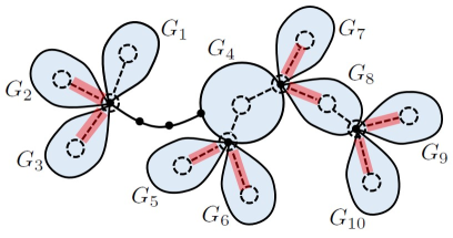
Figure 6: A graph $G$ with $\delta(G)\geq 2$ and ten non-trivial blocks $G_{i}.$ Assuming that all blocks which share a vertex $v$ are $v$-incident, the graph $\Gamma$ of $G$ is shown in dashed line. Graph $\Gamma$ is a forest with two trees, by designating $G_{1}$ and $G_{4}$ as the roots of the corresponding trees of $G,$ a set $E^{\prime}\subseteq E(\Gamma)$ from Claim C within the proof of Theorem 21 is marked in $\Gamma.$

Now we can use the previous two lemmas to state a main result of this section.

Theorem 21

Let $G$ be a graph with $\delta(G)\geq 2.$ Let $G_{1},\ldots,G_{q}$ be all non-trivial blocks in $G.$ Suppose that $\mathrm{dim}(G_{i})\leq 2c(G_{i})-1$ (resp. $\mathrm{edim}(G_{i})\leq 2c(G_{i})-1$) whenever $G_{i}$ is not a cycle. Then $\mathrm{dim}(G)\leq 2c(G)-1$ (resp. $\mathrm{edim}(G)\leq 2c(G)-1$).

Proof. Assume that non-trivial blocks $G_{i}$ of $G$ are denoted so that $G_{i}$ is a cycle if and only if $i>p.$ Then by Lemma 20 we have

$$\mathrm{dim}(G)\leq\mathrm{dim}(G_{1})+\cdots+\mathrm{dim}(G_{q})+p-1.$$

Since the metric dimension of the cycle equals two and since we assumed $\mathrm{dim}(G_{i})\leq 2c(G_{i})-1$ for every $i=1,\ldots,p,$ we further obtain

$$\mathrm{dim}(G) \leq(2c(G_{1})-1)+\cdots+(2c(G_{p})-1)+2(q-p)+p-1=$$

$$=2c(G_{1})+\cdots+2c(G_{q})-p+(q-p)+p-1.$$

Lemma 19 now yields

$$\mathrm{dim}(G)\leq 2c(G)-(q-p)-1\leq 2c(G)-1,$$

and we are finished. The proof for $\mathrm{edim}(G)$ is analogous.    

As for the question when the equality is attained, the proofs of Lemma 20 and Theorem 21 imply the following necessary condition.

Corollary 22

Let $G\not=C_{n}$ be a graph with $\delta(G)\geq 2.$ If $\mathrm{dim}(G_{i})<2c(G_{i})-1$ (resp $\mathrm{edim}(G)\leq 2c(G)-1$) for a block $G_{i}$ of $G$ distinct from a cycle or there exist two vertex-disjoint non-trivial blocks $G_{i}$ and $G_{j}$ in $G$, then $\mathrm{dim}(G)<2c(G)-1$ (resp. $\mathrm{edim}(G)<2c(G)-1$).

As for the role of Theorem 21 in the journey towards the solution of Conjectures 16 and 17 we can state the following.

Corollary 23

If Conjecture 16 (resp. Conjecture 17) holds for all $2$-connected graphs $G$ distinct from $C_{n},$ then it holds in general.

Proof. The claim is the consequence of Theorem 21 and the fact that every non-trivial block in $G$ with $\delta(G)\geq 2$ is a $2$-connected graph.    

5 Concluding remarks

In [15] it was established that the inequalities $\mathrm{dim}(G)\leq L(G)+2c(G)$ and $\mathrm{edim}(G)\leq L(G)+2c(G)$ hold for cacti and it was further conjectured that the same upper bounds hold for metric dimensions of general connected graphs. Noticing that the attainment of these bounds in the class of cacti depends on the presence of the leaves in a graph, in this paper we focused on leafless graphs. In leafless graphs it holds that $L(G)=0,$ so the conjectured upper bound becomes $2c(G).$ We started by characterizing all cacti for which the first smaller upper bound is attained, i.e. $\mathrm{dim}(G)=L(G)+2c(G)-1$ and $\mathrm{edim}(G)\leq L(G)+2c(G)-1.$ A direct consequence of this characterization is that there are some leafless cacti for which this decreased bound is attained. Therefore, in the class of leafless cacti the upper bound $2c(G)-1$ is tight for both metric dimensions.

We conjectured that the decreased upper bound $2c(G)-1$ hols for both metric dimensions of all connected graphs without leaves, i.e. all graphs with $\delta(G)\geq 2$. These conjectures we tested both systematically and stochastically for graphs of smaller order and we did not encounter a counterexample. As a first step towards the solution of this conjecture, we show that it holds for all graphs with $\delta(G)\geq 3$. Also, we showed that if the decreased bound $2c(G)-1$ hold for metric dimensions of $2$-connected graph, then they will also hold for all graphs with $\delta(G)\geq 2,$ i.e. the conjecture will be solved if it is established to hold for $2$-connected graph. Establishing that the conjectured bounds hold for metric dimensions of $2$-connected graphs we leave as an open problem.

Acknowledgments.  Both authors acknowledge partial support of the Slovenian research agency ARRS program P1-0383 and ARRS project J1-1692. The first author also the support of Project KK.01.1.1.02.0027, a project co-financed by the Croatian Government and the European Union through the European Regional Development Fund - the Competitiveness and Cohesion Operational Programme.

References

- [1] P. S. Buczkowski, G. Chartrand, C. Poisson, P. Zhang, On -dimensional graphs and their bases, Period. Math. Hungar. 46(1) (2003) 9–15.
- [2] G. Chartrand, L. Eroh, M. A. Johnson, O. R. Oellermann, Resolvability in graphs and the metric dimension of a graph, Discrete Appl. Math. 105 (2000) 99–113.
- [3] J. Geneson, Metric dimension and pattern avoidance in graphs, Discrete Appl. Math. 284 (2020) 1–7.
- [4] F. Harary, R. A. Melter, On the metric dimension of a graph, Ars Combin. 2 (1976) 191–195.
- [5] A. Kelenc, D. Kuziak, A. Taranenko, I. G. Yero, Mixed metric dimension of graphs, Appl. Math. Comput. 314(1) (2017) 42–438.
- [6] A. Kelenc, N. Tratnik, I. G. Yero, Uniquely identifying the edges of a graph: the edge metric dimension, Discrete Appl. Math. 251 (2018) 204–220.
- [7] S. Khuller, B. Raghavachari, A. Rosenfeld, Landmarks in graphs, Discrete Appl. Math. 70 (1996) 217–229.
- [8] D. J. Klein, E. Yi, A comparison on metric dimension of graphs, line graphs, and line graphs of the subdivision graphs, Eur. J. Pure Appl. Math. 5(3) (2012) 302–316.
- [9] M. Knor, S. Majstorović, A. T. M. Toshi, R. Škrekovski, I. G. Yero, Graphs with the edge metric dimension smaller than the metric dimension, Appl. Math. Comput. 401 (2021) 126076.
- [10] R. A. Melter, I. Tomescu, Metric bases in digital geometry, Comput. Vis. Graph. Image Process. 25 (1984) 113–121.
- [11] I. Peterin, I. G. Yero, Edge metric dimension of some graph operations, Bull. Malays. Math. Sci. Soc. 43 (2020) 2465–2477.
- [12] J. Sedlar, R. Škrekovski, Bounds on metric dimensions of graphs with edge disjoint cycles, Appl. Math. Comput. 396 (2021) 125908.
- [13] J. Sedlar, R. Škrekovski, Extremal mixed metric dimension with respect to the cyclomatic number, Appl. Math. Comput. 404 (2021) 126238.
- [14] J. Sedlar, R. Škrekovski, Mixed metric dimension of graphs with edge disjoint cycles, Discrete Appl. Math. 300 (2021) 1–8.
- [15] J. Sedlar, R. Škrekovski, Vertex and edge metric dimensions of cacti, arXiv:2107.01397 [math.CO].
- [16] J. Sedlar, R. Škrekovski, Vertex and edge metric dimensions of unicyclic graphs, arXiv:2104.00577 [math.CO].
- [17] E. Zhu, A. Taranenko, Z. Shao, J. Xu, On graphs with the maximum edge metric dimension, Discrete Appl. Math. 257 (2019) 317–324.
- [18] N. Zubrilina, On the edge dimension of a graph, Discrete Math. 341(7) (2018) 2083–2088.