Ranked diffusion, delta Bose gas and Burgers equation

Abstract

We study the diffusion of $N$ particles in one dimension interacting via a drift proportional to their rank. In the attractive case (self-gravitating gas) a mapping to the Lieb Liniger quantum model allows to obtain stationary time correlations, return probabilities and the decay rate to the stationary state. The rank field obeys a Burgers equation, which we analyze. It allows to obtain the stationary density at large $N$ in an external potential $V(x)$ (in the repulsive case). In the attractive case the decay rate to the steady state is found to depend on the initial condition if its spatial decay is slow enough. Coulomb gas methods allow to study the final equilibrium at large $N$.

Interacting ranked diffusion, i.e. the diffusion of $N$ particles in 1D under a drift which depends only on their rank were used to model financial or economic data Banner . Pal and Pitman Pitman studied the case where each particle feels a drift $\delta_{j}$ where $j$ is the rank of the particle ($j=1$ is the leftmost one etc..). They showed that the particle spacings converge to independent exponential variables with rates $2\alpha_{j}$, where $\alpha_{j}=\sum_{i=1}^{j}(\delta_{i}-\bar{\delta})$ and $\bar{\delta}$ is the average drift. It holds provided $\alpha_{k}>0$ for all $1\leq k\leq N-1$, i.e. for attractive interactions. They showed connections to reflected Brownian motions in wedges with drifts, generalized by O’Connell and Ortmann OConnell . The large $N$ limit was studied in Jourdain2000 ; JourdainChaosProp2008 ; JourdainReygner2013 ; Reygner2015 ; Pal and shown to be related to a non-linear diffusion process, an example of a more general phenomenon known as propagation of chaos Kac ; McKean ; Sznitman1 ; Sznitman2 ; Calderoni .

Since the Coulomb interaction in 1D is linear in the distance, these models in their stationary state are related to the statistical mechanics of the self-gravitating 1D gas Rybicki ; Kumar2017 (attractive case), or of the 1D Coulomb gas (CG) (repulsive case) in presence of a background charge or in a finite box, also called Jellium Jellium ; SatyaJellium1 ; SatyaJellium2 ; SatyaJellium3 .

In this paper we examine the dynamics of this model, in the light of two exact mappings. (i) The first one, useful for attractive interactions, is to the Lieb-Liniger delta Bose gas model. It allows to obtain the relaxation spectrum for a class of initial conditions with fast enough spatial decay. It also leads some return probabilities, and time dependent correlation functions in the stationary state. (ii) The second is to a Burgers equation with noise, where the noise is subdominant in the large $N$ limit. We use it to determine the stationary state, in the repulsive case in presence of an external potential, as well as the relaxation rate in the attractive case, for initial conditions with slow spatial decay. These lead to a decay rate which depends on the initial condition. Finally we discuss the connection to the Coulomb gas, which allows to determine the true final equilibrium state.

We consider $N$ particles on the real line at positions $x_{i}(t)$ evolving according to the Langevin equation

$$\frac{dx_{i}}{dt}=\bar{c}\sum_{j=1}^{N}{\rm sgn}(x_{j}-x_{i})-V^{\prime}(x_{i})+\sqrt{2T}\xi_{i}(t)$$ (1)

where $\xi_{i}(t)$ are unit independent white noises, $T$ the temperature, and ${\rm sgn}(0)=0$. Here $V(x)$ is an external potential, seen by all walkers. The particles will cross, and we denote $x_{(j)}(t)$ the ordered sequence of their positions at time $t$, i.e. $x_{(1)}(t)\leq x_{(2)}(t)\dots\leq x_{(N)}(t)$. The ordered particle $x_{(j)}$ then feels the permanent drift $\delta_{j}=(N+1-2j)\bar{c}$. The case $\bar{c}>0$ corresponds to attractive interactions and the system (apart from its center of mass) reaches a stationary state even if $V(x)=0$. In the case of repulsive interactions, $\bar{c}<0$, it is useful to add a confining potential, such as an harmonic well, $V(x)=\frac{1}{2}\mu x^{2}$, or a linear trap $V(x)=\mu|x|$, with $\mu>0$.

The probability distribution function (PDF), $P(\vec{x},t)$, of a given configuration, ${\vec{x}}=\{x_{i}(t)\}_{i=1,\dots,N}$, satisfies the Fokker-Planck (FP) equation

$$\partial_{t}P = -{\cal H}_{\rm FP}P$$

$$= \sum_{i}[T\partial_{x_{i}}^{2}+\partial_{x_{i}}(V^{\prime}(x_{i})+\bar{c}\sum_{j}{\rm sgn}(x_{i}-x_{j}))]P$$

It admits a zero current stationary PDF

$$P_{\rm stat}(\vec{x})=\frac{1}{Z_{N}}e^{-\frac{\bar{c}}{2T}\sum_{i,j=1}^{N}|x_{i}-x_{j}|-\frac{1}{T}\sum_{i=1}^{N}V(x_{i})}$$ (3)

which is normalizable on the line when $V(x)$ is a confining potential. In the attractive case, $\bar{c}>0$, and setting $V(x)=0$, one can rewrite footnotecdm

$$P_{\rm stat}(\vec{x})\propto e^{\frac{\bar{c}}{T}\sum_{j=1}^{N}(N+1-2j)x_{(j)}}=e^{-\sum_{j=1}^{N-1}\alpha_{j}(x_{(j+1)}-x_{(j)})}$$ (4)

with $\alpha_{j}=\sum_{i=1}^{j}\delta_{i}/T$ in agreement with Pitman (which uses $T=1/2$) since here $\bar{\delta}=0$. For $\bar{c}<0$ the particles repel each others and one needs a confining potential. In this case $P_{\rm stat}(\vec{x})$ can be interpreted as the equilibrium Gibbs measure of a 1D CG, e.g. as recently studied in SatyaJellium1 ; SatyaJellium2 in the case of the harmonic well.

Mapping to the delta Bose gas. The ranked diffusion (RD) (1) with $V(x)=0$ can be mapped to the Lieb-Liniger (LL) model of delta interacting quantum particles. Defining $\Psi_{0}(\vec{x})=CP_{\rm stat}(\vec{x})^{1/2}$ from (4) footnoteC the FP operator ( Ranked diffusion, delta Bose gas and Burgers equation) relates to a Schrödinger operator ${\cal H}_{s}$ via

$${\cal H}_{\rm FP}=\Psi_{0}{\cal H}^{\prime}_{s}\Psi_{0}^{-1}$$ (5)

where ${\cal H}^{\prime}_{s}={\cal H}_{s}-E_{0}$ and (setting $T=1$ in this section)

$${\cal H}_{s}=-\sum_{i}\partial_{x_{i}}^{2}-2\bar{c}\sum_{1\leq i<j\leq N}\delta(x_{i}-x_{j})$$ (6)

is the Hamiltonian of the LL model LL , with $\bar{c}=-c$ in standard notations. This mapping is useful in the attractive case, $\bar{c}>0$, since the the bound state $\Psi_{0}$ (also called $N$-string) is the ground state of ${\cal H}_{s}$, with energy $E_{0}=-\frac{1}{4}\sum_{i=1}^{N}\delta_{i}^{2}=-\frac{\bar{c}^{2}}{12}(N^{3}-N)$ and zero center of mass momentum. By contrast in the the repulsive case $\bar{c}<0$, it is not the ground state of the LL model footnote2 (for some $V(x)$ it can be related to a quantum model, but with additional interactions SM ). Since for $V(x)=0$ the LL model is integrable, so is the dynamics of the RD system. The Green’s functions $G_{\rm FP/s}=\langle x|e^{-t{\cal H}_{\rm FP/s}}|y\rangle$ are related via

$$G_{\rm FP}(\vec{x},\vec{y},t)=\frac{\Psi_{0}(\vec{x})}{\Psi_{0}(\vec{y})}G_{s}(\vec{x},\vec{y},t)e^{E_{0}t}$$ (7)

and the time dependent PDF of the RD system is obtained from the imaginary time dynamics of the LL model as

$$P(\vec{x},t)=\Psi_{0}(\vec{x}){\cal Z}_{N}(\vec{x},t)e^{E_{0}t}$$ (8)

$${\cal Z}_{N}(\vec{x},t)=\sum_{\lambda}\frac{\langle\Psi_{\lambda}|\Psi(0)\rangle}{||\Psi_{\lambda}||^{2}}\Psi_{\lambda}(\vec{x})e^{-E_{\lambda}t}$$

where the $E_{\lambda}$ are $\Psi_{\lambda}$ are the eigenenergies and the (unnormalized) eigenstates of ${\cal H}_{s}$, given by the Bethe ansatz, and $\langle\vec{x}|\Psi(0)\rangle=\Psi(\vec{x},t=0)=P(\vec{x},0)/\Psi_{0}(\vec{x})$ is the initial condition. For a general initial condition (IC), eigenstates of ${\cal H}_{s}$ with arbitrary symmetry contribute (the model being called Gaudin-Yang GaudinYang ). Choosing a symmetric IC for the RD problem allows to restrict to bosonic eigenstates. One then deduces the relaxation spectrum of the FP operator ( Ranked diffusion, delta Bose gas and Burgers equation) of the RD system as $E_{\lambda}-E_{0}$. The eigenstates m-65 are indexed by the partitions of $N$, i.e. the sets of integers $m_{i}\geq 1$ such that $\sum_{i=1}^{n_{s}}m_{i}=N$, together with wavevectors $k_{i}\in\mathbb{R}$

$$E_{\lambda}=-\frac{\bar{c}^{2}}{12}\sum_{i=1}^{n_{s}}(m_{i}^{3}-m_{i})+\sum_{i=1}^{n_{s}}m_{i}k_{i}^{2}$$ (9)

interpreted as the energy of $1\leq n_{s}\leq N$ bound states, each with $m_{i}$ particles and center of mass momentum $m_{i}k_{i}$. The ground state $\Psi_{0}$ has $n_{s}=1$, $m_{1}=N$ and $k_{1}=0$. We call ”ground state manifold” the space of superpositions of $N$-string eigenstates with momenta $k_{1}=k$, $\Psi_{k}(\vec{x})=e^{ik\sum_{i=1}^{N}x_{i}}\Psi_{0}(\vec{x})$. It is invariant by the dynamics. These superpositions describe the RD system in its stationary state in terms of relative coordinates, together with the free diffusion of the center of mass $\bar{x}=\frac{1}{N}\sum_{i}x_{i}$, i.e. $P(\vec{x},t)\propto\Psi_{0}(\vec{x})^{2}p_{t}(\bar{x})$ with $p_{t}(x)=e^{-(t/N)\partial^{2}_{x}}p_{0}(x)$. In terms of relative coordinates, the lowest excited state has $n_{s}=2$, $m_{1}=N-1$, $m_{2}=1$, i.e. one particle evaporating from the ground state. The convergence to the ground state manifold is thus exponential as $\sim e^{-\gamma_{N}t}$, with relaxation rate

$$\gamma_{N}=\frac{\bar{c}^{2}}{4}N(N-1)$$ (10)

There is a catch however. Eq. (8) holds only insofar the overlaps $\langle\Psi_{\lambda}|\Psi(0)\rangle$ exist, i.e. are given by convergent integrals. This is the case for IC such that $P(\vec{x},0)$ decays sufficiently fast (typically as $\sim\Psi_{0}(\vec{x})$ or faster) at large $\vec{x}$. Then the decay rate is given by (10) and is independent of further details of the IC. Consider e.g. the case $N=2$ which is simple to solve by other methods, and $P(\vec{x},0)\propto e^{-a|x_{1}-x_{2}|}$. One checks SM that for $a>\bar{c}/2$ Eq. (10) holds, while for $a<\bar{c}/2$, one has $\gamma_{2}=2a(\bar{c}-a)$, i.e. the decay is slower and its rate depends on the IC. Although it seems possible to obtain that decay from an analytic continuation of (8), we do not pursue it here. Below we obtain this decay at large $N$ using the Burgers equation, confirming the above predictions.

Sums as ${\cal Z}_{N}(\vec{x},t)$ in (8) have been studied recently in the context of the KPZ equation/directed polymer problem, as recalled in SM . For symmetric IC one has ${\cal Z}_{N}(\vec{x},t)=\mathbb{E}[e^{\sum_{i=1}^{N}h(x_{i},t)}]$, i.e. an average over the noise of the solution $h(x,t)$ of the KPZ equation KPZ such that ${\cal Z}_{N}(\vec{x},t=0)=P(\vec{x},0)/\Psi_{0}(\vec{x})$. The so-called droplet IC thus corresponds to $P(\vec{x},t=0)=\prod_{i}\delta(x_{i})$. Using known results PLDdroplet ; we-flat ; we-flatlong ; flat-shorttime , we display in SM the exact formula for the return probability $P(\vec{0},t)$ in that case, as well as for the IC $P(\vec{x},t=0)\propto\Psi_{0}(\vec{x})$, which corresponds to the flat IC for the KPZ equation. Note that for symmetric IC the propagator $G_{s}(\vec{x},\vec{y},t)$ is known explicitly ProhlacSpohnPropagator .

Finally, one can show that correlation functions in the stationary state of the RD system, such as the two time correlation of the particle density, can be obtained from their analog in the attractive LL model. Using the results of Caux and Calabrese CalabreseCauxBosonsPRL ; CalabreseCauxBosonsLong we display an exact formula for this correlation function in SM .

Mapping to a stochastic Burgers equation. We now turn to a completely different method which applies for any sign of $\bar{c}=-c$ and in presence of an external potential $V(x)$. Let us define the empirical density $\rho$ normalized to unity, $\rho(x,t)=\frac{1}{N}\tilde{\rho}(x,t)$ where $\tilde{\rho}(x,t)=\sum_{i}\delta(x-x_{i}(t))$. Using the Dean-Kawasaki method Dean , one obtains a closed stochastic equation for its evolution, which is exact for any $N$ footnote1

$$\partial_{t}\rho(x,t)=T\partial_{x}^{2}\rho(x,t)+\frac{1}{\sqrt{N}}\partial_{x}[\sqrt{2T\rho(x,t)}\eta(x,t)]$$ (11)

$$+\partial_{x}[V^{\prime}(x)\rho(x,t)+N\bar{c}\rho(x,t)\int dy\rho(y,t){\rm sgn}(x-y))]$$

where $\eta(x,t)$ is a normalized spatial white noise. Now define the rank field $r(x,t)$ through

$$\rho(x,t)=\partial_{x}r(x,t)~{},~{}r(x,t)=\int^{x}_{-\infty}dx^{\prime}\rho(x^{\prime},t)-\frac{1}{2}$$ (12)

which increases monotonically from $-1/2$ at $x=-\infty$ to $+1/2$ at $x=+\infty$. Substituting $\rho(x,t)$ in (11), we use that by integration by part $\int dy\rho(y,t){\rm sgn}(x-y)=2r(x,t)$, since $[r(y,t){\rm sgn}(x-y)]^{y=+\infty}_{y=-\infty}=0$. Integrating once with respect to $x$ we obtain

$$\partial_{t}r(x,t) = T\partial_{x}^{2}r(x,t)+\frac{1}{\sqrt{N}}\sqrt{2T\partial_{x}r(x,t)}\eta(x,t)$$ (13)

$$+ 2N\bar{c}r(x,t)\partial_{x}r(x,t)+V^{\prime}(x)\partial_{x}r(x,t)$$

since the integration constant vanishes from the boundary conditions for $r(x,t)$ at $x=\pm\infty$. If $V(x)=0$ this is the Burgers equation with some multiplicative noise. Note that the function $r(x,t)$ is constrained to be increasing in $x$ (positive density). We now consider the large $N$ limit in two stages.

Large $N$ at fixed $\bar{c}=-c$. If we scale $V(x)=N\tilde{V}(x)$ and rescale time as $t=\tau/N$, we can rewrite (13) as

$$\partial_{\tau}r=2\bar{c}~{}r\partial_{x}r+\tilde{V}^{\prime}(x)\partial_{x}r+\frac{1}{N}\partial_{x}^{2}r+\frac{1}{N}\sqrt{2\partial_{x}r}~{}\tilde{\eta}(x,\tau)$$ (14)

still valid for any $N$, where $\tilde{\eta}$ is another unit white noise (obtained from $\eta$ by the time change). In the limit $N\to+\infty$ we find that $r(x,\tau)$ satisfies (with $c=-\bar{c}$)

$$\partial_{\tau}r=(\tilde{V}^{\prime}(x)-2c~{}r)\partial_{x}r$$ (15)

We now consider separately the repulsive and attractive cases.

In the repulsive case, $c=-\bar{c}>0$, the only singularities can be plateaus where $\partial_{x}r=0$, i.e. regions empty of particles. Setting $\partial_{\tau}r=0$ in (15) we see that around a given $x$ a stationary solution is either constant, $\partial_{x}r=0$, or equal to $r=\frac{1}{2}\tilde{V}^{\prime}(x)/c$, which is acceptable only if $\tilde{V}^{\prime\prime}(x)/c\geq 0$. The simplest case is when $\tilde{V}(x)$ is convex. In that case the stationary solution is unique and given by

$$r_{\rm stat}(x)=\frac{\tilde{V}^{\prime}(x)}{2c}~{},~{}\rho_{\rm stat}(x)=\frac{\tilde{V}^{\prime\prime}(x)}{2c}~{},~{}x_{e}^{-}<x<x_{e}^{+}$$ (16)

and $r_{\rm stat}(x)=\frac{1}{2}{\rm sgn}(x)$ elsewhere. The support of the density is thus an interval and $x_{e}^{\pm}$ are the two edges, given by the roots of $\tilde{V}^{\prime}(x_{e}^{\pm})=\pm c$. The density thus generically has a jump at these edges. This assumes that the potential is sufficiently confining so that the roots $x_{e}^{\pm}$ exist. In the case when $\tilde{V}^{\prime}(+\infty)<c$ and $\tilde{V}^{\prime}(-\infty)>-c$ or both, the edges are pushed to infinity and a finite fraction of the particles are expelled to $\pm\infty$.

For double (or multiple) well types potentials the situation is more involved, since there are regions with $\tilde{V}^{\prime\prime}(x)<0$ where (16) cannot hold. There are thus families of stationary states, which are empty in these regions, leading to multiple intervals support for the density SM .

What is the relaxational dynamics toward stationarity? From (15) we see that $r(x,\tau)$ increases with $\tau$ in regions such that $r<\tilde{V}^{\prime}(x)/2c$ and decreases if $r>\tilde{V}^{\prime}(x)/2c$. In the simplest case it leads to the convergence to the unique stationary solution, Eq. (16). For the double well, the dynamics leads the system to one member of the family of stationary states, which depends on the initial condition $r_{0}(x)=r(x,0)$: it is easily found by noticing that at any point $x=a$ such that $r_{0}(a)=\tilde{V}^{\prime}(a)/2c$, one has $\partial_{\tau}r(a,\tau)=0$, hence $r(a,\tau)=r_{0}(a)$. If at this point $\tilde{V}^{\prime\prime}(a)<0$, $r(x,\tau)$ must develop a plateau around this point in the large time limit, which determines uniquely the stationary state within the family, for details see SM .

The general solution of (15) is obtained by considering $\tau(x,r)$ and using $\frac{\partial_{x}r}{\partial_{\tau}r}=-\partial_{x}\tau$. We obtain $(\tilde{V}^{\prime}(x)-2cr)\partial_{x}\tau=-1$. Let us denote $x_{0}(r)$ the inverse function of the initial condition $r_{0}(x)=r(x,0)$, i.e. $r_{0}(x_{0}(r))=r$. The general solution is then

$$\tau=\int_{x_{0}(r)}^{x}\frac{dy}{2cr-\tilde{V}^{\prime}(y)}$$ (17)

For the harmonic well, $\tilde{V}^{\prime}(y)=\mu_{0}y$, with all particles starting at $x=y$, i.e. $x_{0}(r)=y$, one finds that the density is uniform

$$r(x,\tau)=\frac{\mu_{0}}{2c}\frac{x-ye^{-\mu_{0}\tau}}{1-e^{-\mu_{0}\tau}}~{},~{}\rho(x,\tau)=\frac{\mu_{0}}{2c(1-e^{-\mu_{0}\tau})}$$ (18)

in the time dependent interval $x\in[x_{e}^{-}(\tau),x_{e}^{+}(\tau)]$ with $x_{e}^{\pm}(\tau)=\pm\frac{c}{\mu_{0}}(1-e^{-\mu_{0}\tau})+ye^{-\mu_{0}\tau}$, and zero outside. It converges to the stationary state $\rho_{\rm stat}(x)=\frac{\mu_{0}}{2c}\theta(\frac{c}{\mu_{0}}-|x|)$ as found in the Jellium studies.

For $\tilde{V}(x)=0$ one recovers the perturbative solution of the inviscid Burgers equation

$$2cr\tau=x-x_{0}(r)\quad,\quad r=r_{0}(x-2c\,r\tau)$$ (19)

equivalently $r(x,\tau)=r_{0}(w(x,\tau))$ where

$$w+2c~{}r_{0}(w)\tau=x\quad\Leftrightarrow\quad w=w(x,\tau)$$ (20)

It is valid as long as the map is invertible, i.e. $1+2c\tau\rho_{0}(x)>0$ for all $x$, which always holds for $c>0$. An example is the square density initial condition, $\ell>0$

$$\rho(x,\tau)=\frac{1}{2(\ell+c\tau)}\theta(\ell+c\tau-|x|)$$ (21)

which shows that the repulsive gas expands linearly in time.

Let us consider now the attractive case, $c=-\bar{c}<0$, and focus on $V(x)=0$. Eq. (21) is still valid, but now the gas contracts ballistically and at time $\tau=\ell/\bar{c}$ the density becomes a delta peak at $x=0$ containing all the particles, i.e. $r(x,\tau)$ develops a shock (a step). For more general initial conditions, the perturbative solution fails and a shock appears at time

$$\tau=\tau_{s}=\frac{1}{2\bar{c}\max_{x}\rho(x,0)}$$ (22)

and position $x=x_{s}={\rm argmax}\rho(x,0)$. To describe the dynamics with shocks one recalls that (15) originates from (13). The proper solution is then (see next paragraph), $r(x,\tau)=\frac{w(x,\tau)-x}{2\tau\bar{c}}=r_{0}(w(x,\tau))$ where

$$w(x,\tau):={\rm argmin}_{w\in\mathbb{R}}[\frac{(w-x)^{2}}{4\tau}-\bar{c}\int_{0}^{w}dx^{\prime}r_{0}(x^{\prime})]$$ (23)

which recovers the perturbative solution when there is a single minimum in (23), e.g. for $\bar{c}=-c<0$. For $\bar{c}>0$ (23) leads at intermediate time to one or several shocks, containing finite fractions of the total number of particles, which merge into a single one with unit fraction at some larger time, see SM for details.

Large $N$ with $\gamma=cN$, $\bar{\gamma}=\bar{c}N$ fixed. Going back to (13) one can still neglect the noise but one must keep the diffusion term, leading to

$$\partial_{t}r=T\partial_{x}^{2}r+2\bar{\gamma}~{}r\partial_{x}r+V^{\prime}(x)\partial_{x}r$$ (24)

Although interactions are different, this bears analogy with the studies BouchaudGuionnet of matrix Brownian motion with index $\beta\sim 1/N$, and here too because of the diffusion the stationary density does not vanish anywhere.

Consider first $V(x)=0$. Defining $Z$ a solution of the heat equation, $\partial_{t}Z=T\partial^{2}_{x}Z$, and $r=\frac{T}{\bar{\gamma}}\partial_{x}\log Z$, leads to the Cole-Hopf solution (valid for any sign of $\bar{\gamma}$)

$$r(x,t)=\frac{\int\frac{dw}{\sqrt{4\pi Tt}}\frac{w-x}{2\bar{\gamma}t}e^{-\frac{(w-x)^{2}}{4Tt}+\frac{\bar{\gamma}}{T}\int_{0}^{w}dx^{\prime}r_{0}(x^{\prime})}}{\int\frac{dw}{\sqrt{4\pi Tt}}e^{-\frac{(w-x)^{2}}{4Tt}+\frac{\bar{\gamma}}{T}\int_{0}^{w}dx^{\prime}r_{0}(x^{\prime})}}$$ (25)

where $r_{0}(x)=r(x,0)$ is the initial condition. If one sets $t=\tau/N$ and $\bar{\gamma}=N\bar{c}$ the argument of the exponential is uniformly of $O(N)$ at large $N$ and one recovers the solution of the inviscid Burgers equation (23).

In the attractive case, $\bar{\gamma}>0$, the following initial condition is stationary, $r_{\rm stat}(x)=r(x,t)=r_{0}(x)$ for all $t$

$$\!\!r_{\rm stat}(x)=\frac{1}{2}\tanh(\frac{\bar{\gamma}(x-x_{s})}{2T}),\rho_{\rm stat}(x)=\frac{\bar{\gamma}}{4T\cosh^{2}(\frac{\bar{\gamma}(x-x_{s})}{2T})}$$ (26)

and describes a shock at position $x_{s}$ containing all the particles, which, in this scaling, has a finite width $O(T/\bar{\gamma})$. It perfectly agrees with the large $N$ limit of the finite $N$ density profile associated to the IC $P_{N}(\vec{x},0)\propto\Psi_{0}(\vec{x})^{2}\delta(\bar{x}-x_{s})$, which in Fourier reads $\hat{\rho}^{s}_{N}(K)=\prod_{a=1}^{N-1}(1+(\frac{K}{N\bar{c}a})^{2})^{-1}\to_{N\to\infty}\frac{\pi K}{\bar{\gamma}\sinh(\pi K/\bar{\gamma})}$ as first calculated in Rybicki . Note that the diffusion of the shock center, ${\rm Var}\,x_{s}(t)\sim\frac{2T}{N}t$ is subdominant, and only observable on larger time scales $t\sim N$.

Using the solution to Burgers equation (25) one can investigate again the question of the decay rate towards (26). One finds that fast decaying IC have decay rate $\bar{\gamma}^{2}/4$ consistent with the large $N$ limit of (10). On the other hand, one can solve e.g. the case of two packets, $r_{0}(x)=\frac{p_{1}}{2}\tanh(\frac{p_{1}\bar{\gamma}}{2}(x-x_{1}))+\frac{p_{2}}{2}\tanh(\frac{p_{2}\bar{\gamma}}{2}(x-x_{2}))$, with $p_{1}+p_{2}=1$, which leads a decay rate $p_{1}p_{2}\bar{\gamma}^{2}\leq\frac{1}{4}\bar{\gamma}^{2}$ SM .

In the repulsive case $\gamma=-\bar{\gamma}>0$, let us investigate the quadratic potential $V(x)=\mu\frac{x^{2}}{2}$. Eq. (24) can be put in the form of a Burgers equation with friction $\mu$ SM . We only study the stationary solution. Its support is the whole real axis, and it takes the scaling form

$$r_{\rm stat}(x)=\frac{\sqrt{\mu T}}{2\gamma}\hat{r}_{g}(x\sqrt{\frac{\mu}{T}})~{},~{}\rho_{\rm stat}(x)=\frac{\mu}{2\gamma}\hat{\rho}_{g}(x\sqrt{\frac{\mu}{T}})$$ (27)

where $\hat{r}_{g}(y)=y-R_{g}(y)$, $\hat{\rho}_{g}(y)=1-R_{g}^{\prime}(y)$ are a one parameter family of scaling functions indexed by $g=\gamma/\sqrt{\mu T}$, which measures the relative strength of interaction and potential energies. The odd dimensionless function $R_{g}(y)$ is the solution of $0=R_{g}^{\prime\prime}+R_{g}R_{g}^{\prime}-R_{g}$ such that $R_{g}(y)\simeq y\mp g$ for $y\to\pm\infty$. This autonomous equation is solved by writing $R^{\prime}=w(R)$. The solution for $\hat{\rho}_{g}(y)$ is obtained by eliminating $R$ and $b>0$ between

$$\!\!\hat{\rho}_{g}(y)=-W(-e^{-b-1-\frac{R^{2}}{2}}),\int_{0}^{R}\frac{du}{1+W(-e^{-b-1-\frac{u^{2}}{2}})}=y$$

$$\int_{0}^{+\infty}du\big{(}\frac{1}{1+W(-e^{-b-1-\frac{u^{2}}{2}})}-1\big{)}=g$$ (28)

where $W(z)$ is the main branch of the Lambert function, solution of $z=We^{W}$, with $z>e^{-1}$ and $W(e^{-1})=-1$. In the limit $g\to 0$, $b$ is large and using $W(z)=\sum_{n\geq 1}\frac{(-n)^{n-1}}{n!}z^{n}$ one obtains the expansion $\hat{\rho}_{g}(y)=\sqrt{\frac{2}{\pi}}ge^{-\frac{y^{2}}{2}}+O(g^{2})$ around the Gaussian shape in the absence of interactions $\gamma=0$, see SM . Similarly, for $g\to+\infty$, $b\to 0^{-}$ and in the scale $y\sim g$ the scaling function takes a square form $\hat{\rho}_{g}(y)\simeq\theta(1-\frac{y}{g})$.

Coulomb gas. The Dean-Kawasaki equation (11) satisfies detailed balance Dean ; DeanPrivate , with the energy

$$H[\rho] = \frac{\bar{c}N^{2}}{2}\int dxdx^{\prime}|x-x^{\prime}|\rho(x)\rho(x^{\prime})+N\int dxV(x)\rho(x)$$ (29)

$$+ TN\int dx\rho(x)\log\rho(x)$$

the last term being the entropy term, see SM for details, and one expects that the system reaches equilibrium with Gibbs measure ${\cal P}_{\rm stat}[\rho]\propto\exp\left(-H[\rho]/T\right)$. In the first large $N$ limit, at fixed $c=-\bar{c}$, with $V(x)=N\tilde{V}(x)$, one has $H[\rho]\simeq N^{2}{\cal E}[\rho]$ and only the first two terms in (29) contribute. Consider repulsive interactions $c>0$. We have checked SM that for convex potentials, minimization of ${\cal E}[\rho]$ gives the same solution as the asymptotic state (16) of the dynamics (15). The Coulomb gas in that regime (in a quadratic well) was studied in the context of Jellium: it was shown that at very low temperature $T\sim 1/N$, the system almost cristallizes, and that the rightmost particle has position fluctuations $O(1/N)$, obtained in SatyaJellium1 ; SatyaJellium2 .

For double well potentials and $c>0$, the density has two supports and we find SM that the minimizer is only one special member of the family of steady states reached by the dynamics on the fast time scales $\tau=Nt=O(1)$. Not so surprisingly, barrier crossing is needed to equilibrate the two wells, a process which occurs on much larger time scales, and would be interesting to study. For $\bar{c}>0$ the minimizer is a single delta function packet (shock) at the position of the minimum of $\tilde{V}(x)$.

Finally, in the large $N$ limit with fixed $\gamma=Nc$ all three term in (29) are $O(N)$ and contribute, with $H[\rho]\simeq N{\cal E}_{2}[\rho]$. Minimization of ${\cal E}_{2}[\rho]$ recovers the stationary equation associated to (24).

In conclusion we studied the dynamics of interacting ranked diffusion in 1D using the tools of the integrable LL model (for attractive interactions) and of the Burgers equation (for both cases, most useful in the large $N$ limit). Stationary solutions, decay rates and stationary correlations were obtained. For IC with fast spatial decay, the decay rate in time is universal and given by the LL Hamiltonian spectrum, while it is continuously varying and slower for IC which decay slowly in space. The Coulomb gas allows to obtain the equilibrium state on much larger time scales. Since the Burgers equation describes the large $N$ dynamics (with $\gamma=N\bar{c}$ fixed) on the same time scales as the LL model (in imaginary time) it would be interesting to explore the correspondence further.

Acknowledgments: I am grateful to S. N. Majumdar for useful interactions at the early stages of this work. I thank J. Quastel and L.C. Tsai for discussions on relations to the Burgers equation, and D. Dean for sharing notes. This research was supported by ANR grant ANR-17-CE30-0027-01 RaMaTraF.

.

We give the details of the calculations described in the main text of the Letter, and display some of the more lengthy results (in particular the return probabilities and stationary correlations within the Bethe ansatz, as well as some explicit solutions to Burgers equation).

I Associated quantum model

Inserting $P=\Psi_{0}\Psi$ in the Fokker-Planck equation ( Ranked diffusion, delta Bose gas and Burgers equation) in the text, one finds that $\Psi$ satisfies the imaginary time Schrödinger equation

$$\partial_{t}\Psi=-{\cal H}^{\prime}_{s}\Psi=\left(\sum_{i}\partial_{x_{i}}^{2}+\frac{1}{2}\sum_{i}\partial_{x_{i}}F_{i}-\frac{1}{4}\sum_{i}F_{i}^{2}\right)\Psi\quad,\quad F_{i}=V^{\prime}(x_{i})+\bar{c}\sum_{j}{\rm sgn}(x_{i}-x_{j})$$ (30)

For $V(x)=0$ one obtains the Lieb-Liniger Hamiltonian

$${\cal H}^{\prime}_{s}=-\sum_{i}\partial_{x_{i}}^{2}-2\bar{c}\sum_{1\leq i<j\leq N}\delta(x_{i}-x_{j})-E_{0}\quad,\quad E_{0}=-\frac{\bar{c}^{2}}{4}\sum_{i=1}^{N}(N+1-2i)^{2}=-\frac{\bar{c}^{2}}{12}(N^{3}-N)$$ (31)

The ground state of ${\cal H}^{\prime}_{s}$ is $\Psi_{0}$ with zero energy. The standard LL model has Hamiltonian ${\cal H}_{s}={\cal H}^{\prime}_{s}+E_{0}$ and has ground state energy $E_{0}$.

For interacting ranked diffusion (RD) in presence of an external potential $V(x)$ the associated quantum model is not the Lieb-Liniger model anymore, but there are additional one and two body terms i.e. ${\cal H}_{s}\to{\cal H}_{s}+\delta{\cal H}_{s}$ with

$$\delta{\cal H}_{s}=\frac{1}{4}\sum_{i}(V^{\prime}(x_{i})^{2}-2V^{\prime\prime}(x_{i}))+\frac{\bar{c}}{4}\sum_{i,j}(V^{\prime}(x_{i})-V^{\prime}(x_{j})){\rm sgn}(x_{i}-x_{j})$$ (32)

For RD in the quadratic potential $V(x)=\frac{1}{2}\mu x^{2}$ the additional terms in the quantum model are

$$\delta{\cal H}_{s}=-\frac{\mu N}{2}+\frac{\mu^{2}}{4}\sum_{i}x_{i}^{2}+\frac{\mu\bar{c}}{4}\sum_{i,j}|x_{i}-x_{j}|$$ (33)

i.e. a quadratic well and a linear attraction.

For RD in the linear trap $V(x)=\mu|x|$ one finds

$$\delta{\cal H}_{s}=\frac{N}{4}\mu^{2}-\mu\sum_{i}\delta(x_{i})+\frac{\bar{c}\mu}{4}(N^{2}-(\sum_{i}{\rm sgn}(x_{i}))^{2})$$ (34)

II Bethe ansatz solution for the ranked diffusion dynamics

II.1 General symmetric initial condition

We use the quantum mechanical notations for states $|\Psi\rangle$, and their associated wavefunctions in coordinate basis $\Psi(\vec{x})=\langle\vec{x}|\Psi\rangle$. The scalar product is $\langle\Phi|\Psi\rangle=\int dx_{1}\dots dx_{N}\Phi^{*}(\vec{x})\Psi(\vec{x})$ and the norm square is $||\Psi||^{2}=\langle\Psi|\Psi\rangle$.

The un-normalized symmetric eigenfunctions of the LL Hamiltonian ${\cal H}_{s}$ in (6) with attractive interactions ($\bar{c}>0$) on the infinite line are built m-65 ; GaudinBook by partitioning the $N$ particles into a set of $1\leq n_{s}\leq N$ bound states called strings each formed by $m_{j}\geq 1$ particles with $N=\sum_{j=1}^{n_{s}}m_{j}$. In the sector $x_{1}\leq x_{2}\leq\dots\leq x_{N}$ they read

$$\Psi_{\lambda}(\vec{x})=\sum_{P\in S_{N}}A_{P}\prod_{j=1}^{N}e^{i\sum_{\alpha=1}^{N}\lambda_{P_{\alpha}}x_{\alpha}}\,,\quad A_{P}=\prod_{1\leq\alpha<\beta\leq N}\Big{(}1+\frac{i\bar{c}}{\lambda_{P_{\beta}}-\lambda_{P_{\alpha}}}\Big{)}\,.$$ (35)

which involves a sum over permutations $P$ in $S_{N}$. The rapidities are

$$\lambda_{j,a}=k_{j}-\frac{i\bar{c}}{2}(m_{j}+1-2a)\quad,\quad j=1,\dots n_{s}\quad,\quad a=1,...,m_{j}$$ (36)

where $k_{j}$ is a real momentum, the total momentum of the string being $K_{j}=m_{j}k_{j}$. One denotes equivalently $|\Psi_{\lambda}\rangle\equiv|\Psi_{{\bf k},{\bf m}}\rangle$ these strings states, and $\Psi_{\lambda}(\vec{x})=\Psi_{{\bf k},{\bf m}}(\vec{x})$ the corresponding eigenfunctions, labelled by the set of $k_{j},m_{j}$, $j=1,..n_{s}$. The eigenenergies are

$$E_{\lambda}=\sum_{\alpha=1}^{N}\lambda_{\alpha}^{2}=E({\bf k},{\bf m})\quad,\quad E({\bf k},{\bf m}):=\sum_{j=1}^{n_{s}}m_{j}k_{j}^{2}-\frac{\bar{c}^{2}}{12}(m_{j}^{3}-m_{j})$$ (37)

and the inverse norms are CalabreseCauxBosonsPRL ; CalabreseCauxBosonsLong ; Kirillov

$$\frac{1}{||\Psi_{{\bf k},{\bf m}}||^{2}}=\frac{\bar{c}^{N}}{N!(\bar{c}L)^{n_{s}}}\Phi({\bf k},{\bf m})\prod_{j=1}^{n_{s}}\frac{1}{m_{j}^{2}}\quad,\quad\Phi({\bf k},{\bf m})=\prod_{1\leq i<j\leq n_{s}}\frac{4(k_{i}-k_{j})^{2}+(m_{i}-m_{j})^{2}\bar{c}^{2}}{4(k_{i}-k_{j})^{2}+(m_{i}+m_{j})^{2}\bar{c}^{2}}$$ (38)

This formula is valid on a ring of size $L$ as $L\to+\infty$. When summing over states the factors of $L$ cancel in that limit, upon using the quantification of the total string momenta $\sum_{k_{j}}\to Lm_{j}\int\frac{dk}{2\pi}$. See e.g. we-flatlong for more details (same conventions).

On the infinite line this leads to the following exact expression for the ranked diffusion probability, which we denote $P_{N}(\vec{x},t)$, with a symmetric initial condition $P_{N}(\vec{x},0)$

$$P_{N}(\vec{x},t)=\Psi_{0}(\vec{x}){\cal Z}_{N}(\vec{x},t)e^{E_{0}t}$$ (39)

where the sum over states in (8) in the text takes the form

$${\cal Z}_{N}(\vec{x},t)=\sum_{n_{s}=1}^{N}\frac{\bar{c}^{N-n_{s}}}{n_{s}!N!}\prod_{j=1}^{n_{s}}\sum_{m_{j}\geq 1}\int\frac{dk_{j}}{2\pi m_{j}}\delta_{N,\sum_{j=1}^{n_{s}}m_{j}}\Phi({\bf k},{\bf m})e^{-tE({\bf k},{\bf m})}\Psi_{{\bf k},{\bf m}}(\vec{x})\langle\Psi(0)|\Psi_{{\bf k},{\bf m}}\rangle$$ (40)

Here the state $|\Psi(0)\rangle$ is the initial condition of the quantum evolution and reads in the coordinate basis, together with the overlap

$$\langle\vec{x}|\Psi(0)\rangle=\frac{P_{N}(\vec{x},0)}{\Psi_{0}(\vec{x})}\quad,\quad\langle\Psi(0)|\Psi_{{\bf k},{\bf m}}\rangle=\int d^{N}\vec{x}\,\frac{P_{N}(\vec{x},0)}{\Psi_{0}(\vec{x})}\Psi_{{\bf k},{\bf m}}(\vec{x})$$ (41)

We will assume here that these overlap integrals exist, which assumes that the spatial decay of $P_{N}(\vec{x},0)$ at large $\vec{x}$ is sufficiently fast, as discussed in the text.

Ground state. The ground state is a single $N$-string with $k_{1}=0$ and $m_{1}=N$, i.e

$$\Psi_{0}(\vec{x})=\Psi_{0,N}(\vec{x})=N!e^{\frac{\bar{c}}{2}\sum_{a=1}^{N}(N+1-2a)x_{(a)}}=N!e^{-\frac{\bar{c}}{2}\sum_{1\leq i<j\leq N}|x_{i}-x_{j}|}$$ (42)

and energy $E_{0}=E(0,N)=-\frac{\bar{c}^{2}}{12}(N^{3}-N)$. Its square norm is $||\Psi_{0}||^{2}=N!N^{2}L\bar{c}^{1-N}$, where the factor of $L$ comes from integration over the (free) center of mass coordinate.

Ground state manifold

There is a manifold of eigenstates which plays a special role, let us call it the ground state manifold. It corresponds to $n_{s}=1$ and consists of superpositions of single $N$-string states but with arbitrary momentum, with associated wave functions $\Psi_{k,N}(\vec{x})=\Psi_{0}(\vec{x})e^{ik\sum_{i}x_{i}}$. It has two properties. First if the initial condition belongs to this manifold it remains inside and its dynamics then describes the time evolution of the center of mass. Second, for any initial condition, we expect that the evolution will converge at large time to this manifold.

Separating the term $n_{s}=1$ in (40) and inserting into (39) we see that we can write

$$P(\vec{x},t)=P^{n_{s}=1}(\vec{x},t)+P^{n_{s}\geq 2}(\vec{x},t)$$ (43)

where the first term evolves inside the ground state manifold and reads

$$P^{n_{s}=1}(\vec{x},t)=\Psi_{0}(\vec{x})^{2}\frac{\bar{c}^{N-1}}{N!}\int\frac{dk}{2\pi N}e^{-tNk^{2}}e^{ik\sum_{i}x_{i}}\langle\Psi(0)|\Psi_{k,N}\rangle$$ (44)

and where the overlap is

$$\langle\Psi(0)|\Psi_{k,N}\rangle=\int d^{N}\vec{x}P(\vec{x},0)e^{-ik\sum_{i}x_{i}}$$ (45)

Suppose first that the initial condition is of the product form

$$P_{N}(\vec{x},0)=\frac{\bar{c}^{N-1}}{N!N^{2}}\Psi_{0}(\vec{x})^{2}\,p_{0}(\frac{1}{N}\sum_{i}x_{i})$$ (46)

i.e. it is stationary in the particle relative positions, with a decoupled form for the center of mass. Then it is easy to see that it remains of this form. Indeed, defining the Fourier transform $\tilde{p}_{0}(K)$ of the initial PDF $p_{0}(x)$ for the center of mass as

$$p_{0}(x)=\int\frac{dK}{2\pi}e^{iKx}\tilde{p}_{0}(K)$$ (47)

one can rewrite the initial condition as (setting $K=Nk$ the total string momentum)

$$P_{N}(\vec{x},0)=\frac{\bar{c}^{N-1}}{N!N^{2}}\Psi_{0}(\vec{x})^{2}\int\frac{dk}{2\pi}e^{ik\sum_{i}x_{i}}\hat{p}_{0}(k)\quad,\quad\hat{p}_{0}(k)=N\tilde{p}_{0}(Nk)$$ (48)

and one sees that $P_{N}(\vec{x},0)/\Psi_{0}(x)$ belongs to the ground state manifold. Let us check that its evolution is indeed simple, from the above formula (44). Let us compute the overlap (45) from (48). One obtains

$$\langle\Psi(0)|\Psi_{k,N}\rangle=\frac{\bar{c}^{N-1}}{N!N^{2}}\int d^{N}\vec{x}\int\frac{dq}{2\pi}\Psi_{0}(\vec{x})^{2}e^{i(q-k)\sum_{i}x_{i}}\hat{p}_{0}(q)=\frac{1}{N}\hat{p}_{0}(k)$$ (49)

where we have used that $\delta_{k,0}=\frac{2\pi}{LN}\delta(k)$, hence that

$$\int d^{N}\vec{x}\Psi_{0}(\vec{x})^{2}e^{ik\sum_{i}x_{i}}=||\Psi_{0}||^{2}\delta_{k,0}=||\Psi_{0}||^{2}\frac{2\pi}{LN}\delta(k)=N!N\bar{c}^{1-N}2\pi\delta(k)$$ (50)

Inserting the overlap in (44) leads to

$$P_{N}(\vec{x},t)=\frac{\bar{c}^{N-1}}{N!N^{2}}\Psi_{0}(x)^{2}\int\frac{dk}{2\pi}e^{ik\sum_{i}x_{i}}\hat{p}_{0}(k)e^{-Nk^{2}t}=\frac{\bar{c}^{N-1}}{N!N^{2}}\Psi_{0}(\vec{x})^{2}\times p_{t}(\frac{1}{N}\sum_{i}x_{i})$$ (51)

where $p_{t}(x)$ is the PDF of the center of mass at time $t$

$$p_{t}(x)=\int\frac{dK}{2\pi}e^{iKx}\tilde{p}_{0}(K)e^{-\frac{K^{2}}{N}t}$$ (52)

The center of mass performs diffusion with variance $\frac{2}{N}t$. Note that if $\int dx\,p_{0}(x)=\tilde{p}_{0}(0)=1$ then $P_{N}(\vec{x},t)$ is normalized to unity for all $t$ (see subsection below).

Consider now an initial condition which is not of this form. As mentionned in the text there is a gap in the energy spectrum between states with $n_{s}\geq 2$ and with $n_{s}=1$, of value $\gamma_{N}=\frac{\bar{c}^{2}}{4}N(N-1)$. Hence we expect a convergence of the form $\sim e^{-\gamma_{N}t}$ towards the ground state manifold, i.e. $P_{N}(\vec{x},t)\simeq P^{n_{s}=1}(\vec{x},t)$ for times $t\gg 1/\gamma_{N}$. As discussed in the text this holds provided the overlaps are convergent integrals, i.e. if the spatial decay of $P_{N}(\vec{x},0)$ at infinity is fast enough.

As an example let us consider as in the text the ”droplet” initial condition

$$P_{N}(\vec{x},0)=\prod_{i=1}^{N}\delta(x_{i})$$ (53)

which is normalized to unity. The overlap is now $\langle\Psi(0)|\Psi_{k,N}\rangle=1$ and one obtains from the above the large time behavior

$$P_{N}(\vec{x},t)\simeq P^{n_{s}=1}(\vec{x},t)=\frac{\bar{c}^{N-1}}{N!N^{2}}\Psi_{0}(x)^{2}\,p_{t}(\frac{1}{N}\sum_{i}x_{i})\quad,\quad p_{t}(x)=\frac{\sqrt{N}}{\sqrt{4\pi t}}e^{-N\frac{x^{2}}{4t}}$$ (54)

Note that at intermediate time all excited states contribute and the dynamics is more complicated.

Separation of the center of mass motion

It is possible to separate completely the center of mass coordinate $x$ from the relative coordinate variables. If the following factorized form holds at time $t=0$, it holds at all time

$$P_{N}(\vec{x},t)=p_{t}(x)P_{t}(\vec{y})\quad,\quad x=\frac{1}{N}\sum_{i=1}^{N}x_{i}\quad,\quad y_{i}=x_{i}-x$$ (55)

The normalization condition $\int d^{N}\vec{x}P_{N}(\vec{x},t)=1$ is satisfied if

$$\int dx\,p_{t}(x)=1\quad,\quad\int d^{N}\vec{y}\,\,\delta(\frac{1}{N}\sum_{i=1}^{N}y_{i})P_{t}(\vec{y})=1$$ (56)

As can be seen by using that $\int d^{N}\vec{x}=\int dx\int d^{N}\vec{x}\delta(x-\frac{1}{N}\sum_{i=1}^{N}x_{i})=\int dx\int d^{N}\vec{y}\delta(\frac{1}{N}\sum_{i=1}^{N}y_{i})$ upon shifting $x_{i}=y_{i}+x$.

To show (55) for all time, note that setting $x_{i}=x+y_{i}$ in the expression for the eigenstates (35), (36) they take the form

$$\Psi_{{\bf k},{\bf m}}(\vec{x})=e^{i\sum_{j=1}^{n_{s}}k_{j}m_{j}x}\Psi_{{\bf k},{\bf m}}(\vec{y})$$ (57)

Inserting $\int dx\delta(x-\frac{1}{N}\sum_{i}x_{i})=1$ in the expression of the overlap (41) one obtains

$$\langle\Psi(0)|\Psi_{{\bf k},{\bf m}}\rangle=\tilde{p}_{0}(\sum_{j=1}^{n_{s}}m_{j}k_{j})\langle\Psi(0)|\Psi_{{\bf k},{\bf m}}\rangle_{y}$$ (58)

$$\tilde{p}_{0}(K):=\int dxe^{iKx}p_{0}(x)\quad,\quad\langle\Psi(0)|\Psi_{{\bf k},{\bf m}}\rangle_{y}:=\int d^{N}\vec{y}\,\delta(\frac{1}{N}\sum_{i=1}^{N}y_{i})\,\frac{P_{0}(\vec{y})}{\Psi_{0}(\vec{y})}\Psi_{{\bf k},{\bf m}}(\vec{y})$$ (59)

Inserting into (40) one obtains

$$P_{N}(\vec{x},t)=\int\frac{dK}{2\pi}e^{iKx}\tilde{p}_{0}(K)$$ (60)

$$\times\Psi_{0}(\vec{y})\sum_{n_{s}=1}^{N}\frac{\bar{c}^{N-n_{s}}}{n_{s}!N!}\prod_{j=1}^{n_{s}}\sum_{m_{j}\geq 1}\int\frac{dk_{j}}{2\pi m_{j}}\delta_{N,\sum_{j=1}^{n_{s}}m_{j}}(2\pi)\delta(K-\sum_{j=1}^{n_{s}}m_{j}k_{j})\Phi({\bf k},{\bf m})e^{-t(E({\bf k},{\bf m})-E_{0})}\Psi_{{\bf k},{\bf m}}(\vec{y})\langle\Psi(0)|\Psi_{{\bf k},{\bf m}}\rangle_{y}$$

Now one notes that shifting the integration variables as $k_{j}=k+q_{j}$, all terms inside the integral are invariant except the constraint $\delta(K-\sum_{j=1}^{n_{s}}k_{j}m_{j})\to\delta(K-Nk-\sum_{j=1}^{n_{s}}m_{j}q_{j})$ and the energy $E({\bf k},{\bf m})=Nk^{2}+2k\sum_{j=1}^{n_{s}}m_{j}q_{j}+\sum_{j=1}^{n_{s}}m_{j}q_{j}^{2}$. If we choose $k=K/N$ the expression for the energy decouples and one finally obtains (55) with

$$p_{t}(x)=\int\frac{dK}{2\pi}e^{iKx}\tilde{p}_{0}(K)e^{-\frac{K^{2}}{N}t}$$ (61)

$$P_{t}(\vec{y})=\Psi_{0}(\vec{y})\sum_{n_{s}=1}^{N}\frac{\bar{c}^{N-n_{s}}}{n_{s}!N!}\prod_{j=1}^{n_{s}}\sum_{m_{j}\geq 1}\int\frac{dq_{j}}{2\pi m_{j}}\delta_{N,\sum_{j=1}^{n_{s}}m_{j}}(2\pi)\delta(\sum_{j=1}^{n_{s}}m_{j}q_{j})\Phi({\bf q},{\bf m})e^{-t(E({\bf q},{\bf m})-E_{0})}\Psi_{{\bf q},{\bf m}}(\vec{y})\langle\Psi(0)|\Psi_{{\bf q},{\bf m}}\rangle_{y}$$

II.2 Probability of presence at the origin

The formula (39), (40) are exact but the Bethe eigenfunctions become quite complicated for higher values of $n_{s}$. A simpler observable is the probability of presence at the origin.

Droplet initial condition. Let us consider again the initial condition (53) where all particles are at $x=0$ at time $t=0$ and ask the probability at time $t$, $P(\vec{x}=0,t)(dx)^{N}$ that they are all in a small volume $(dx)^{N}$ around the origin. In that case it is a return probability.

We insert in (39), (40) the exact value of the Bethe wavefunctions (35) at coinciding points $\Psi_{\lambda}(\vec{0})=N!$ and of the overlap with the initial state, which consequently equals unity, $\langle\Psi(0)|\Psi_{{\bf k},{\bf m}}\rangle=1$, and obtain

$$P(\vec{x}=0,t)=N!e^{E_{0}t}\sum_{n_{s}=1}^{N}\frac{\bar{c}^{N-n_{s}}}{n_{s}!}\prod_{j=1}^{n_{s}}\sum_{m_{j}\geq 1}\int\frac{dk_{j}}{2\pi m_{j}}\delta_{N,\sum_{j=1}^{n_{s}}m_{j}}e^{t\sum_{j=1}^{n_{s}}[\frac{\bar{c}^{2}}{12}(m_{j}^{3}-m_{j})-m_{j}k_{j}^{2}]}\prod_{1\leq i<j\leq n_{s}}\frac{4(k_{i}-k_{j})^{2}+(m_{i}-m_{j})^{2}\bar{c}^{2}}{4(k_{i}-k_{j})^{2}+(m_{i}+m_{j})^{2}\bar{c}^{2}}$$

For instance one finds $P_{1}(0,t)=\int\frac{dk}{2\pi}e^{-k^{2}t}=\frac{1}{\sqrt{4\pi t}}$ and

$$P_{2}(\vec{0},t)=\bar{c}\int\frac{dk}{2\pi}e^{-2k^{2}t}+e^{-\frac{1}{2}\bar{c}^{2}t}\int\frac{dk_{1}}{2\pi}\int\frac{dk_{2}}{2\pi}e^{-k_{1}^{2}t-k_{2}^{2}t}\frac{(k_{1}-k_{2})^{2}}{(k_{1}-k_{2})^{2}+\bar{c}^{2}}=\frac{2e^{-\frac{\bar{c}^{2}t}{2}}+\sqrt{2\pi}\bar{c}\sqrt{t}\left(\text{erf}\left(\frac{\bar{c}\sqrt{t}}{\sqrt{2}}\right)+1\right)}{8\pi t}$$ (62)

where ${\rm erf}(z)=\frac{2}{\sqrt{\pi}}\int_{0}^{z}dte^{-t^{2}}$, and so on for higher $N$. This coincides with the result for the moments of the KPZ equation with droplet initial conditions, $P_{N}(\vec{0},t)=e^{E_{0}t}\overline{Z(0,t)^{N}}=e^{E_{0}t}\overline{e^{Nh(0,t)}}$, as obtained in PLDdroplet (see Eqs. (9)-(11) there). Here $h(x,t)$ is the height field which obeys the KPZ equation $\partial_{t}h=\partial_{x}^{2}h+(\partial_{x}h)^{2}+\sqrt{2\bar{c}}\eta(x,t)$ where $\eta(x,t)$ a standard white noise (which is averaged over). Denoting $Z(x,t)=e^{h(x,t)}$ the droplet initial condition is $Z(x,t=0)=\delta(x)$.

For general $N$ the return probability $P_{N}(\vec{0},t)$ interpolates between $P_{N}(\vec{0},t)\simeq P_{1}(0,t)^{N}$ at short time and $P_{N}(\vec{0},t)\simeq\bar{c}^{N-1}N!\frac{1}{N\sqrt{4\pi Nt}}$ at large time.

Flat initial condition. Another initial condition of interest is

$$P_{N}(\vec{x},t=0)=C_{N}\Psi_{0}(\vec{x})$$ (63)

If we choose $C_{N}=(\bar{c}/2)^{N-1}/(N!N^{2}L)$, then it is normalized to $\int d^{N}\vec{x}P(\vec{x},0)=1$, i.e. with a uniform density for the center of mass. In the KPZ context corresponds to the flat IC $Z(x,t=0)=1$ with ${\cal Z}_{N}(\vec{0},t)=C_{N}\overline{Z(0,t)^{N}}$, hence the probability density of presence at the origin

$$P_{N}(\vec{0},t)=N!e^{E_{0}t}C_{N}\overline{Z(0,t)^{N}}$$ (64)

The moments $\overline{Z(0,t)^{N}}$ have been obtained in we-flat ; we-flatlong . For $N\leq 4$ explicit formula where given in we-flatlong ; flat-shorttime . Using these formula we obtain

$$P_{2}(\vec{0},t)=2C_{2}\left(1+{\rm erf}(\bar{c}\frac{\sqrt{t}}{\sqrt{2}})\right)$$ (65)

which increases by a factor of $2$ between $t=0$ and $t=+\infty$. Next we obtain

$$P_{3}(\vec{0},t)=6C_{3}\left(4-2e^{-\frac{3}{2}\bar{c}^{2}t}-2{\rm erfc}(\bar{c}\sqrt{2t})+e^{-\frac{3}{2}\bar{c}^{2}t}{\rm erfc}(\bar{c}\frac{\sqrt{t}}{\sqrt{2}})\right)$$ (66)

which increases by a factor of $4$ between $t=0$ and $t=+\infty$. Finally one has

$$P_{4}(\vec{0},t)=4!C_{4}\bigg{(}8-8e^{-3\bar{c}^{2}t}-4{\rm erfc}(\frac{3}{\sqrt{2}}\bar{c}\sqrt{t})+8e^{-3\bar{c}^{2}t}{\rm erfc}(\bar{c}\sqrt{t})-4{\rm erfc}(2\bar{c}\sqrt{t})$$

$$+48e^{-5\bar{c}^{2}t}\int_{0}^{\infty}dx\frac{\left(\frac{2x+1}{\sqrt{4x+1}}-\frac{\sqrt{2x+1}}{x+1}\right)e^{-2\bar{c}^{2}tx}}{4\pi(4x(x+3)+5)}\bigg{)}$$ (67)

which increases by a factor of $8$ between $t=0$ and $t=+\infty$. For general $N$ similar formula can be obtained and the increase between $t=0$ and $t=+\infty$ is $2^{N-1}$.

Note that the flat IC is the limiting case where the overlap integrals exist.

Finally, there are also results for Brownian initial conditions for the KPZ equation, These corresponds to more exotic initial conditions for the RD problem

$$P_{N}(\vec{x},0)\propto\Psi_{0}(\vec{x})\mathbb{E}[e^{\sum_{j=1}^{N}\sqrt{\bar{c}}B(x_{j})}]$$ (68)

where $B(x)$ is a two sided Brownian motion in $x$ with $B(0)=0$, with possibly two different drifts $w_{L,R}$ on each side. It can be made more explicit using and

$$\mathbb{E}e^{\sum_{j=1}^{p}B(-y_{j})}=e^{-\frac{\bar{c}}{2}\sum_{j=1}^{p}(2j-1)y_{j}}\quad,\quad y_{1}<..<y_{p}<0$$ (69)

$$\mathbb{E}e^{\sum_{j=1}^{p}B(y_{j})}=e^{\frac{\bar{c}}{2}\sum_{j=1}^{p}(2p-2j+1)y_{j}}\quad,\quad 0<y_{1}<..<y_{p}$$ (70)

We have not attempted to study this case, but it may be of interest. The overlap integrals will require analytic continuations, since the spatial decay is slower than for the flat IC.

II.3 Correlation functions

Consider an observable, for instance the density (here normalized to $N$ so we use the notation $\tilde{\rho}$ of the main text)

$${\tilde{\rho}}(x;\vec{x})=\sum_{i}\delta(x-x_{i})$$ (71)

Its expectation value in the stationary state of the RD system, i.e. $P_{N}(\vec{x},0)=\Psi_{0}(\vec{x})^{2}/||\Psi_{0}||^{2}$ (which is normalized to unity), is given by

$$\langle{\tilde{\rho}}(x;\vec{x}(0))\rangle=\int d^{N}\vec{x}{\tilde{\rho}}(x;\vec{x})\frac{\Psi_{0}(\vec{x})^{2}}{||\Psi_{0}||^{2}}=\frac{\langle\Psi_{0}|\hat{\rho}(x,0)|\Psi_{0}\rangle}{||\Psi_{0}||^{2}}$$ (72)

where $\hat{\rho}(x,0)$ is the density operator corresponding to the observable (71). Hence it is equal to the quantum expectation of the density operator in the ground state of the LL model. Note that in that state the center of mass has uniform probability over the system hence the result is simply $N/L$. We will study below the more interesting case where the center of mass position is fixed.

Consider now a time dependent correlation in the RD system. It can be expressed as a quantum matrix element in imaginary time. Indeed one has

$$\langle{\tilde{\rho}}(x,t){\tilde{\rho}}(y,0)\rangle=\langle{\tilde{\rho}}(x;\vec{x}(t)){\tilde{\rho}}(y;\vec{x}(0))\rangle=\int d^{N}\vec{x}\int d^{N}\vec{y}{\tilde{\rho}}(x;\vec{x})G_{FP}(\vec{x},\vec{y},t){\tilde{\rho}}(y;\vec{y})P_{N}(\vec{y},0)$$ (73)

$$=e^{E_{0}t}\int d^{N}\vec{x}\int d^{N}\vec{y}\Psi_{0}(\vec{x}){\tilde{\rho}}(x;\vec{x})G_{s}(\vec{x},\vec{y},t){\tilde{\rho}}(y;\vec{y})\langle\vec{y}|\Psi(0)\rangle$$ (74)

$$=\langle\Psi_{0}|\hat{\rho}(x,t)\hat{\rho}(y,0)|\Psi(0)\rangle$$ (75)

where $\hat{\rho}(x,t)$ is the density operator in the Heisenberg representation, i.e. $\hat{\rho}(x,t)=e^{\hat{H}_{s}t}\hat{\rho}(x,0)e^{-\hat{H}_{s}t}$ in imaginary time (with $t=i\tau$ and $\tau$ is quantum real time).

For instance consider the time correlation of the density in the stationary state of the RD system, which corresponds to the initial (unnormalized) quantum state $\langle\vec{y}|\Psi(0)\rangle=\Psi_{0}(\vec{y})/||\Psi_{0}||^{2}$. This gives

$$C(x-y,t):=\langle{\tilde{\rho}}(x,t){\tilde{\rho}}(y,0)\rangle=\frac{\langle\Psi_{0}|\hat{\rho}(x,t)\hat{\rho}(y,0)|\Psi_{0}\rangle}{||\Psi_{0}||^{2}}$$ (76)

This relation extends to any number of space-times points, although we will focus here on two points. It extends in fact to any operator, for instance it also applies to correlations of the fields operator $\Phi^{\dagger}(x)$ and $\Phi(x)$ which insert an additional particle, or respectively remove it. The correlations of this operator were computed in CalabreseCauxBosonsPRL ; CalabreseCauxBosonsLong but we will not study it here.

The stationary dynamics are thus related in both systems. To make it explicit one defines the form factors $\Sigma^{\rho}_{\lambda}$ of the density operator between the ground state and an arbitrary eigenstate $|\Psi_{\lambda}\rangle$ of the LL Hamiltonian

$$\langle\Psi_{0}|\hat{\rho}(x)|\Psi_{\lambda}\rangle=\Sigma^{\rho}_{\lambda}e^{iK_{\lambda}x}$$ (77)

where $K_{\lambda}$ is the total momentum of the eigenstate $|\Psi_{\lambda}\rangle$. The two point stationary density correlation function $C(x,t)$ in the RD system can then be expressed using these form factors as a sum over intermediate eigenstates $\Psi_{\lambda}$

$$C(x,t)=\frac{\langle\Psi_{0}|\hat{\rho}(x,t)\hat{\rho}(0,0)|\Psi_{0}\rangle}{||\Psi_{0}||^{2}}=\sum_{\lambda}\frac{|\Sigma^{\rho}_{\lambda}|^{2}}{||\Psi_{0}||^{2}||\Psi_{\lambda}||^{2}}e^{-(E_{\lambda}-E_{0})t+iK_{\lambda}x}$$ (78)

$$=\sum_{n_{s}=1}^{N}\frac{\bar{c}^{2N-1-n_{s}}}{n_{s}!N!^{2}N^{2}L}\prod_{j=1}^{n_{s}}\sum_{m_{j}\geq 1}\int\frac{dk_{j}}{2\pi m_{j}}\delta_{N,\sum_{j=1}^{n_{s}}m_{j}}\Phi({\bf k},{\bf m})|\Sigma^{\rho}_{{\bf k},{\bf m}}|^{2}e^{ix\sum_{j=1}^{n_{s}}m_{j}k_{j}-t(E({\bf k},{\bf m})-E_{0})}$$ (79)

The explicit expressions for these form factors were obtained by Calabrese and Caux CalabreseCauxBosonsPRL ; CalabreseCauxBosonsLong and we can thus apply their results. One has, in our conventions,

$$|\Sigma^{\rho}_{\lambda}|=\frac{N!}{\bar{c}^{N}}\frac{(\sum_{j}m_{j}k_{j})^{2}}{\bar{c}}N!(N-1)!\prod_{j=1}^{n_{s}}H_{m_{j}}(k_{j}/\bar{c})\quad,\quad H_{m}(x)=|\frac{\Gamma(\frac{N-m}{2}+ix)}{\Gamma(\frac{N+m}{2}+ix)}|^{2}$$ (80)

Let us give the explicit result for $N=2$ and perform some checks. We write

$$\langle{\tilde{\rho}}(x,t){\tilde{\rho}}(y,0)\rangle=\int\frac{dK}{2\pi}e^{iK(x-y)}C(K,t)$$ (81)

Performing the sum over states in (79) we obtain the correlation for $N=2$ in Fourier space

$$C(K,t)=\frac{4}{L}\frac{\bar{c}^{4}}{(\frac{1}{4}K^{2}+\bar{c}^{2})^{2}}e^{-\frac{1}{2}tK^{2}}+\frac{64\bar{c}^{3}e^{-\frac{1}{2}\bar{c}^{2}t}}{L}K^{4}e^{-\frac{1}{2}tK^{2}}\int\frac{dq}{2\pi}\frac{e^{-\frac{1}{2}tq^{2}}}{((q+K)^{2}+\bar{c}^{2})^{2}((q-K)^{2}+\bar{c}^{2})^{2}}\frac{q^{2}}{q^{2}+\bar{c}^{2}}$$ (82)

where the first term arises from the intermediate excited state $\lambda$ being a $2$-string (with total momentum $K=2k_{1}$) and the second term from the two $1$-strings (with total momentum $K=k_{1}+k_{2}$).

There are two important sum rules which allow to check the result. The first one is obtained by integrating (81) over $x$ which gives

$$C(K=0,t)=\int dx\langle{\tilde{\rho}}(x,t){\tilde{\rho}}(0,0)\rangle=N\langle{\tilde{\rho}}(0,0)\rangle=2\frac{2}{||\Psi_{0}||^{2}}\int dy_{2}\Psi_{0}(y,y_{2})^{2}=\frac{4}{L}$$ (83)

and is indeed satisfied by (82). The second is the so-called f-sum rule CalabreseCauxBosonsPRL ; CalabreseCauxBosonsLong . It is obtained by noticing that $[[\hat{H},{\tilde{\rho}}_{K}],{\tilde{\rho}}_{-K}]=-\sum_{j}[[\partial_{x_{j}},e^{iKx_{j}}],e^{-iKx_{j}}]=-2NK^{2}$ where ${\tilde{\rho}}_{K}=\sum_{j}e^{iKx_{j}}$. Taking its expectation in the ground state leads to

$$-L\partial_{t}C(K,t)|_{t=0}=\sum_{\lambda}(E_{\lambda}-E_{0})\frac{|\langle\Psi_{\lambda}|\hat{\rho}_{K}|\Psi_{0}\rangle|^{2}}{||\Psi_{\lambda}||^{2}||\Psi_{0}||^{2}}=NK^{2}$$ (84)

From (82) one finds that the sum of the two contributions indeed simplifies into

$$-L\partial_{t}C(K,t)|_{t=0}=2K^{2}\frac{\bar{c}^{4}}{(\frac{1}{4}K^{2}+\bar{c}^{2})^{2}}+2K^{4}\frac{K^{2}+8\bar{c}^{2}}{16\left(K^{2}+4\bar{c}^{2}\right)^{2}}=2K^{2}$$ (85)

$N$-string contribution to the density correlation

For general $N$ there are many terms in the sum (79). We can see already on (82) that in the large time limit at fixed $K$ the $2$-string (the ground state manifold) dominates.

For the $N$-string for any $N$, of total momentum $Nk$, one has from (80)

$$\Sigma_{k}^{\rho}=\frac{N!N^{3}}{\bar{c}^{N-1}}\frac{1}{\prod_{a=1}^{N-1}(1+(\frac{k}{\bar{c}a})^{2})}$$ (86)

This leads to the following contribution of the ground state manifold to the density correlation function

$$C(K,t)|_{\rm N-string}=\frac{N^{2}e^{-\frac{1}{N}K^{2}t}}{L\prod_{a=1}^{N-1}(1+(\frac{K}{N\bar{c}a})^{2})^{2}}$$ (87)

which saturates the sum rule $C(0,t)=N^{2}/L$ and which we expect to dominate in the large time limit for any $N$ at fixed $K$. In the next subsection we give an interpretation for this result in terms of shocks.

Large $N$ limit . In the large $N$ limit with $g=N\bar{c}$ fixed one has

$$C(K,t)|_{\rm N-string}\simeq\frac{N^{2}(\pi K/g)^{2}e^{-\frac{1}{N}K^{2}t}}{L\sinh(\pi K/g)^{2}}$$ (88)

which saturates the sum rule CalabreseCauxBosonsPRL ; CalabreseCauxBosonsLong

$$\int\frac{dK}{2\pi}C(K,t)|_{\rm N-string}\simeq\frac{N^{3}\bar{c}}{6L}$$ (89)

In Ref. CalabreseCauxBosonsPRL ; CalabreseCauxBosonsLong more excited states are considered, i.e. the two string states $N-M$, $M$. At fixed $N$, this captures some of the finite time behavior (but not all since there are many more possible excited states). However it was found that including already simply $M=1$ saturates the $f$ sum rule at large $N$. That may be an indication of how to recover the full Burgers dynamics from the LL Hamiltonian, but we leave this to future investigations.

Localized center of mass

One would also like to study the correlation functions in the RD system with a slightly more general initial condition of the type (46) (i.e. in the ground state manifold) with a non-uniform distribution for the center of mass position

$$P_{N}(\vec{x},0)=\frac{\bar{c}^{N-1}}{N!N^{2}}\Psi_{0}(\vec{x})^{2}\,p_{0}(\frac{1}{N}\sum_{i}x_{i})=\frac{NL}{||\Psi_{0}||^{2}}\int\frac{dk}{2\pi}\tilde{p}_{0}(Nk)\Psi_{0}(\vec{x})\Psi_{k}(\vec{x})$$ (90)

where in the last equality we used (48) and $\Psi_{k}(\vec{x})=e^{ik\sum_{i}x_{i}}\Psi_{0}(\vec{x})$, as well as the Fourier transform $\tilde{p}_{0}(K)=\int dxe^{-iKx}p_{0}(x)$. A case of special interest is $p_{0}(x)=\delta(x)$ where the center of mass is at a fixed position, with $\tilde{p}_{0}(K)=1$.

The mean density is already non trivial, and can be expressed using the form factor $\Sigma^{\rho}_{k}$ associated to the $N$-string with total momentum $K=Nk$

$$\langle{\tilde{\rho}}(x,0)\rangle=\int d^{N}\vec{x}\,{\tilde{\rho}}(x;\vec{x})P_{N}(\vec{x},0)=NL\int\frac{dk}{2\pi}\tilde{p}_{0}(Nk)\frac{\langle\Psi_{0}|\hat{\rho}(x)|\Psi_{k}\rangle}{||\Psi_{0}||^{2}}=NL\int\frac{dk}{2\pi}\tilde{p}_{0}(Nk)e^{iNkx}\frac{\Sigma^{\rho}_{k}}{||\Psi_{0}||^{2}}$$ (91)

Inserting the result (86) we obtain

$$\langle\tilde{\rho}(x,0)\rangle=N\langle\rho(x)\rangle=N\int\frac{dK}{2\pi}\tilde{p}_{0}(K)e^{iKx}\frac{1}{\prod_{a=1}^{N-1}(1+(\frac{K}{N\bar{c}a})^{2})}$$ (93)

which is properly normalized $\int dx\langle{\tilde{\rho}}(x)\rangle=N$, since $\int dxp(x)=\tilde{p}_{0}(0)=1$. In the particular case of $p_{0}(x)=\delta(x)$ (i.e. center of mass fixed at the origin) this is the result obtained by Rybicki in the context of the self-gravitating gas Rybicki , as recalled in the text. Note that it is simply obtained from the density form factor.

In the large $N$ limit at fixed $\bar{c}$ one finds $\langle\rho(x,0)\rangle=p_{0}(x)$ (i.e the width of the packet can be neglected).

In the large $N$ limit at fixed $\bar{\gamma}=N\bar{c}$, using

$$\frac{1}{\prod_{a=1}^{N-1}(1+(\frac{x}{a})^{2})}=\frac{\pi x}{\sinh(\pi x)}+\frac{\pi x^{3}}{N\sinh(\pi x)}+O(N^{-2})$$ (94)

One finds

$$\langle\rho(x,0)\rangle\simeq\int\frac{dK}{2\pi}\tilde{p}_{0}(K)e^{iKx}\frac{\pi K}{\bar{\gamma}\sinh(\frac{\pi}{\bar{\gamma}}K)}$$ (95)

In the case of fixed center of mass position, $p(x)=\delta(x)$, inverting the Fourier transform one finds

$$\langle\rho(x,0)\rangle\simeq\frac{\bar{\gamma}}{4\cosh^{2}(\frac{\bar{\gamma}}{2}x)}$$ (96)

This is precisely the density profile obtained below in (160) as the stationary solution of the Burgers equation and corresponding to a single shock centered at $x=0$ and containing all the particles.

When the center of mass has initial distribution $p_{0}(x)$ both the finite $N$ result (93) and its large $N$ limit (95) can be written as a convolution

$$\langle\rho(x)\rangle\simeq\int dx_{s}\,p_{0}(x_{s})\rho^{s}_{N}(x-x_{s})\quad,\quad\rho^{s}_{\infty}(x)=\frac{\bar{\gamma}}{4\cosh^{2}(\frac{\bar{\gamma}}{2}(x-x_{s}))}$$ (97)

which can be interpreted as a superposition of a group of $N$ particles centered at random positions $x_{s}$. Here $\rho^{s}_{N}(x)$ is the finite $N$ density profile of the group, and $\rho^{s}_{\infty}(x)$ its large $N$ limit, which becomes the stationary shock in the Burgers picture.

Correlation at different times. Reproducing the steps in (73) we now obtain the two time density correlation of the RD system with the initial condition (90) as

$$\langle\tilde{\rho}(x,t)\tilde{\rho}(y,0)\rangle=\frac{NL}{||\Psi_{0}||^{2}}\int\frac{dk}{2\pi}\tilde{p}_{0}(Nk)\langle\Psi_{0}|\hat{\rho}(x,t)\hat{\rho}(y,0)|\Psi_{k}\rangle$$ (98)

It can be written again as a sum involving form factors of the LL model

$$\langle\tilde{\rho}(x,t)\tilde{\rho}(y,0)\rangle=\frac{NL}{||\Psi_{0}||^{2}}\int\frac{dk}{2\pi}\tilde{p}_{0}(Nk)\sum_{\lambda}\frac{1}{||\Psi_{\lambda}||^{2}}\langle\Psi_{0}|\hat{\rho}(0)|\Psi_{\lambda}\rangle\langle\Psi_{\lambda}|\hat{\rho}(0)|\Psi_{k}\rangle e^{iNky+iK_{\lambda}(x-y)}e^{-(E_{\lambda}-E_{0})t}$$ (99)

where we used that $\langle\Psi_{\lambda}|\hat{\rho}(y)|\Psi_{k}\rangle=e^{i(Nk-K_{\lambda})y}\langle\Psi_{\lambda}|\hat{\rho}(0)|\Psi_{k}\rangle$.

We will only give here the contribution of the ground state manifold

$$\langle\rho(x,t)\rho(y,0)\rangle|_{\rm N-string}=\int\frac{dK}{2\pi}\tilde{p}_{0}(K)\int\frac{dP}{2\pi}\frac{e^{iKy+iP(x-y)-\frac{1}{N}P^{2}t}}{\prod_{a=1}^{N-1}(1+(\frac{P}{N\bar{c}a})^{2})\prod_{a=1}^{N-1}(1+(\frac{K-P}{N\bar{c}a})^{2})}$$ (100)

For any $N$ it can be rewritten as as a superposition of packets of particles with a random center

$$\langle\rho(x,t)\rho(y,0)\rangle|_{\rm N-string}=\mathbb{E}_{\omega}\left(\int dx_{s}\,p_{0}(x_{s})\rho_{N}^{s}(y-x_{s})\rho_{N}^{s}(x-x_{s}-\sqrt{\frac{2t}{N}}\omega)\right)$$ (101)

where $\omega$ is a unit Gaussian random variable. This shows that the ground state manifold (i.e. the $N$-string contribution) captures only the diffusion of the center of mass, i.e. the position of the shock, averaged over its initial position. In the large $N$ limit one can neglect that diffusion, which corresponds to neglecting the noise in the Burgers equation. The ground state manifold then only captures the correlation due to the random initial position of the shock.

Note that the Burgers dynamics in the large $N$ limit contains much more information on time scales of order unity. It is the information contained in the excited states of the LL whose energy above the ground state scale as $\sim N^{2}\bar{c}^{2}=\bar{\gamma}^{2}$ and remains finite in that limit (and are larger or equal to the gap $\gamma_{N}\simeq\frac{1}{4}\bar{c}^{2}N^{2}=\frac{1}{4}\bar{\gamma}^{2}$).

II.4 Limitations of the mapping

To investigate the decay rate to the stationary state of the RD system, in this subsection we solve directly the case $N=2$ in the repulsive case $\bar{c}>0$, setting $T=1$. The Langevin equation reads

$$\dot{x}_{1}=\bar{c}\,{\rm sgn}(x_{2}-x_{1})+\sqrt{2}\xi_{1}(t)\quad,\quad\dot{x}_{2}=\bar{c}\,{\rm sgn}(x_{1}-x_{2})+\sqrt{2}\xi_{2}(t)$$ (102)

Let us denote $x(t)=\frac{1}{2}(x_{1}(t)+x_{2}(t))$ and $y(t)=x_{2}(t)-x_{1}(t)$. While the center of mass performs an independent unit Brownian motion, $\dot{x}(t)=\xi(t)$, the relative coordinate evolves as

$$\dot{y}=-2\bar{c}\,{\rm sgn}(y)+2\eta(t)$$ (103)

where $\eta(t)$ is an independent unit white noise. Its probability density $P(y,t)$ then evolves according to

$$\partial_{t}P=2\partial_{y}^{2}P+2\bar{c}\partial_{y}({\rm sgn}(y)P)$$ (104)

Introducing the Laplace transform $\tilde{P}(y,s)=\int_{0}^{+\infty}dtP(y,t)$ one obtains

$$s\tilde{P}-P(y,0)=2\partial_{y}^{2}\tilde{P}+2\bar{c}\partial_{y}({\rm sgn}(y)\tilde{P})$$ (105)

where $P(y,0)$ is the initial condition.

Let us choose a simple (even) initial condition, $P(y,0)=\frac{a}{2}e^{-a|y|}$ where $a>0$. It is then easy to solve separately for $y>0$ and $y<0$. There are two integration constants on both sides. One on each side is set to zero by requiring that $\tilde{P}(y,s)\to 0$ at $y\to\pm\infty$ for $s>0$. Continuity of $P$ at $y=0$ gives another condition and finally, from integrating (104) on a small interval around $y-0$ one obtains the matching condition

$$P^{\prime}(0^{+},t)-P^{\prime}(0^{-},t)+2\bar{c}P(0,t)=0$$ (106)

and the same relation holds for the Laplace transforms.

For simplicity of notations let us choose units so that $\bar{c}=1$. This leads to the unique solution

$$\tilde{P}(y,s)=\frac{1}{s+2a(1-a)}\left(\frac{a}{2}e^{-a|y|}+\frac{a(1-a)}{\sqrt{1+2s}-1}e^{-\frac{1}{2}(1+\sqrt{1+2s})|y|}\right)$$ (107)

The first term is a special solution of (105), in real time

$$P_{s}(y,t)=\frac{a}{2}e^{-a|y|}e^{-2a(1-a)t}$$ (108)

which however does not obey the matching condition (106), except for $a=1$ in which case it is the stationary solution

$$P_{\rm stat}(y)=\frac{1}{2}e^{-|y|}$$ (109)

Returning to the case of general $a$ let us invert the Laplace transform at $y=0$. One finds

$$P(0,t)=\frac{1}{4}\left((2a-1)e^{2(a-1)at}\left(\text{erf}\left(\frac{(1-2a)\sqrt{t}}{\sqrt{2}}\right)+1\right)+\text{erf}\left(\frac{\sqrt{t}}{\sqrt{2}}\right)+1\right)$$ (110)

There is a transition in the large time behavior at $a=1/2$. For $a\neq 1/2$ one finds as $t\to+\infty$

$$P(0,t)=\frac{1}{2}+e^{-\frac{t}{2}}\left(\frac{a(a-1)\sqrt{2}}{(1-2a)^{2}\sqrt{\pi}t^{3/2}}+O(t^{-5/2})\right)-\frac{1}{2}(1-2a)e^{-2a(1-a)t}\,\theta(a<\frac{1}{2})$$ (111)

where the asymptotic value is $P_{\rm stat}(0)=1/2$. For $a>1/2$ this decay is consistent with the result from the LL model with decay rate $\gamma_{2}=\frac{1}{2}$. For $a<1/2$ there is an additional contribution with a slower decay rate $2a(1-a)\leq\frac{1}{2}$. At the transition point $a=1/2$ one finds

$$P(0,t)=\frac{1}{4}\left(\text{erf}\left(\frac{\sqrt{t}}{\sqrt{2}}\right)+1\right)=\frac{1}{2}+e^{-\frac{t}{2}}\left(-\frac{1}{2\sqrt{2\pi t}}+\frac{1}{2\sqrt{2\pi}t^{3/2}}+O(t^{-5/2})\right)$$ (112)

For completeness we gives also $P(y,t)$ from Laplace inversion. One finds for any $a$

$$P(y,t)=\frac{1}{2}ae^{-2(1-a)at-a|y|}$$ (113)

$$\frac{1}{4}e^{-|y|}\left(-ae^{(a-1)(2at-|y|)}\text{erfc}\left(\frac{-4at+2t+|y|}{2\sqrt{2}\sqrt{t}}\right)+(a-1)e^{a(2(a-1)t+|y|)}\text{erfc}\left(\frac{4at-2t+|y|}{2\sqrt{2}\sqrt{t}}\right)+\text{erfc}\left(\frac{|y|-2t}{2\sqrt{2}\sqrt{t}}\right)\right)$$

At the transition point $a=1/2$ it simplifies into

$$P(y,t)=\frac{1}{4}e^{-|y|}\left(e^{\frac{|y|-t}{2}}\text{erf}\left(\frac{|y|}{2\sqrt{2}\sqrt{t}}\right)+\text{erfc}\left(\frac{|y|-2t}{2\sqrt{2}\sqrt{t}}\right)\right)$$ (114)

Interestingly we see that (113) at fixed $y,t$ is nicely analytic in $a$ across $a=1/2$. Hence there is a way to extract the result in the regime $a<1/2$ from the LL, presumably by analytic continuation of the overlap integrals (i.e. by moving the contours of integration on the string momenta $k_{j}$). We leave that study to the future.

General initial condition. Note that the general even initial condition can be solved by introducing $\hat{P}(\mu,s)=\int_{0}^{+\infty}dye^{-\mu y}\tilde{P}(y,s)$. Denoting $P_{0}(\mu)=\int_{0}^{+\infty}dye^{-\mu y}P(y,0)$, the Laplace transform of the initial condition, one obtains

$$s\hat{P}(\mu,s)-P_{0}(\mu)=2\mu(1+\mu)\hat{P}(\mu,s)-2\tilde{P}^{\prime}(0,s)-2(1+\mu)P(0,s)$$ (115)

and we want to impose $P^{\prime}(0,s)+P(0,s)=0$. The solution is

$$\hat{P}(\mu,s)=\frac{P_{0}(\mu)-2\mu\tilde{P}(0,s)}{s-2\mu(1+\mu)}$$ (116)

To determine the unknown function $\tilde{P}(0,s)$ one notes that there should not be a pole at $s=2\mu(1+\mu)$. Indeed since $\mu>0$ that would lead to a Laplace inverse diverging exponentially with time. Hence one has

$$\tilde{P}(0,s=2\mu(1+\mu))=\frac{P_{0}(\mu)}{2\mu}$$ (117)

Equivalently, setting $\mu=\frac{1}{2}(\sqrt{1+2s}-1)$ (the positive root) one must have

$$\tilde{P}(0,s)=\frac{P_{0}(\mu=\frac{1}{2}(\sqrt{1+2s}-1))}{\sqrt{1+2s}-1}$$ (118)

In the case of the above initial condition $P_{0}(\mu)=\frac{a}{2}\frac{a}{a+\mu}$, Laplace inverting in $\mu$ one recovers the above results. In that case the large time decay rate can be obtained as $-2\mu(1+\mu)$ with $\mu=-a$ the pole of $P_{0}(\mu)$. Presumably this is a general feature, with $\mu$ being the smallest singularity of the Laplace transform of the initial condition.

LL calculation

Let us compare with the prediction from the LL model for $N=2$. We set $\bar{c}=1$. We recall that $\Psi_{0}(\vec{x})=2e^{-\frac{1}{2}|x_{2}-x_{1}|}$. The initial condition is

$$P_{2}(x_{1},x_{2},t)=\frac{a}{2}e^{-a|y|}p_{0}(x)$$ (119)

with $y=x_{2}-x_{1}$ and $x=\frac{x_{1}+x_{2}}{2}$. The contribution of the $2$-string is simply

$$P|_{n_{s}=1}(x,y,t)=\frac{1}{2}e^{-|y|}p_{t}(x)\quad,\quad p_{t}(x)=\int\frac{dK}{2\pi}e^{iKx-\frac{1}{2}K^{2}t}\tilde{p}_{0}(K)$$ (120)

where $\tilde{p}_{0}(K)=\int dxe^{-iKx}p_{0}(x)$. The overlap integral with the ground state always exists, and does not generate any condition on the decay of the initial PDF of $y$.

The contribution of the two $1$-strings is, with the definitions $k_{1}=k-q/2$, $k_{2}=k+q/2$

$$P|_{n_{s}=2}(x,y,t)=\frac{1}{2}e^{-\frac{1}{2}|y|}e^{-t/2}\int\frac{dk}{2\pi}\frac{dq}{2\pi}\frac{q^{2}}{q^{2}+1}e^{-2k^{2}t-\frac{q^{2}}{2}t}\Psi_{k_{1},k_{2},1,1}(x,y)\langle\Psi(0)|\Psi_{k_{1},k_{2},1,1}\rangle$$ (121)

where

$$\Psi_{k_{1},k_{2},1,1}(x,y)=e^{2ikx}\phi_{q}(y)\quad,\quad\phi_{q}(y)=e^{\frac{1}{2}iq|y|}(1+\frac{i}{q})+e^{-\frac{1}{2}iq|y|}(1-\frac{i}{q})$$ (122)

The overlap exists, strictly speaking, only for $a>1/2$ and is then equal to

$$\langle\Psi(0)|\Psi_{k_{1},k_{2},1,1}\rangle=\int d^{N}\vec{x}\frac{P_{2}(\vec{x},t=0)}{\Psi_{0}(\vec{x})}\Psi^{*}_{k_{1},k_{2},1,1}(\vec{x})=[\int dx^{\prime}e^{-2ikx^{\prime}}p_{0}(x^{\prime})]\times\int dy^{\prime}\frac{a}{4}e^{-(a-\frac{1}{2})|y|}\phi^{*}_{q}(y)$$ (123)

$$=\tilde{p}_{0}(2k)\frac{4a(a-1)}{q^{2}+(2a-1)^{2}}$$ (124)

Thus we obtain

$$P|_{n_{s}=2}(x,y,t)=P|_{n_{s}=2}(y,t)p_{t}(x)~{},~{}P|_{n_{s}=2}(y,t)=a(a-1)e^{-\frac{1}{2}|y|-t/2}\int\frac{dq}{2\pi}\frac{1}{q^{2}+(2a-1)^{2}}\frac{q^{2}e^{-\frac{q^{2}}{2}t}}{q^{2}+1}(e^{\frac{1}{2}iq|y|}(1+\frac{i}{q})+c.c)$$ (125)

To compute these integrals we use

$$e^{-\frac{q^{2}}{2}t}=\frac{1}{\sqrt{2\pi}}e^{iqu\sqrt{t}-u^{2}/2}$$ (126)

The integral over $q$ can then be easily obtained from mathematica Fourier transform routine and the result integrates explicitly over $u$ in terms of error functions. Putting both contributions together one obtains exactly the result (113) obtained by the direct method, although here its derivation is valid only for $a>1/2$.

III Large $N$ at fixed $\bar{c}$: inviscid Burgers dynamics

As in the text we first consider the limit of large $N$ at fixed $\bar{c}$, and scale $V(x)=N\tilde{V}(x)$ and rescale time as $t=\tau/N$. In this limit the dynamics is described by the equation (15) in the text. This first-order PDE can exhibit two common types of singularities (recalling that $\partial_{x}r\geq 0$):

(i) intervals $[x^{-}(\tau),x^{+}(\tau)]$ empty of particles, where $r(x,\tau)=r_{p}$ has a plateau (i.e. $\rho(x,\tau)=0$). The reciprocal function $x(r,\tau)$ (used below) has a jump at $r=r_{p}$. Note that the value of the plateau $r_{p}$ is time independent (as long as the plateau exists).

(ii) shocks at $x=x_{s}(\tau)$ where $r$ exhibits a upward jump $r(x_{s}^{\pm},\tau)=r^{\pm}(\tau)$ where a macroscopic fraction $r^{+}(\tau)-r^{-}(\tau)>0$ of particles accumulate and the density has a delta peak. There the reciprocal function $x(r,\tau)$ (used below) has a plateau on $[r^{-}(\tau),r^{+}(\tau)]$

While empty regions can exist for both signs of $c$, shocks occurs in the dynamics when $\bar{c}<0$.

III.1 Repulsive interactions $c=-\bar{c}>0$

Let us write in that case with $c>0$

$$\partial_{\tau}r(x,\tau)=\left(\tilde{V}^{\prime}(x)-2c~{}r(x,\tau)\right)\partial_{x}r(x,\tau)$$ (127)

To interpret the term in factor let us note that from the definition (12) of the rank field the original Langevin equation (1) can be rewritten in these rescaled variables as

$$\dot{x}_{i}=\frac{d}{d\tau}x_{i}(\tau)=2c\,r(x_{i}(\tau),\tau)-\tilde{V}^{\prime}(x_{i}(\tau))+\frac{\sqrt{2T}}{\sqrt{N}}\tilde{\xi}_{i}(\tau)$$ (128)

where $\tilde{\xi}(\tau)$ is a unit white noise. Thus neglecting the noise term at large $N$ one sees that the prefactor in (127) is simply $-\dot{x}$.

Setting $\partial_{\tau}r=0$ in (15) we see that around a given $x$ a stationary solution $r_{\rm stat}(x)$ is either constant, with $r_{\rm stat}^{\prime}(x)=0$, e.g. part of an empty interval, or equal to $r_{\rm stat}(x)=\frac{1}{2}\tilde{V}^{\prime}(x)/c$, which is acceptable only if $\tilde{V}^{\prime\prime}(x)\geq 0$.

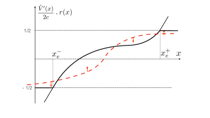
Figure 1: Light black: plot of $\tilde{V}^{\prime}(x)/(2c)$ versus $x$, convex potential case. Thick black: stationary rank function $r_{\rm stat}(x)$. The support of the density $r^{\prime}_{\rm stat}(x)$ is a single interval $[x_{e}^{-},x_{e}^{+}]$. Dashed red: initial $r_{0}(x)$. Red arrows indicate the variation of $r(x,t)$ with time ($\dot{r}$ has opposite sign to $\dot{x}$)

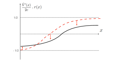
Figure 2: Light black: plot of $\tilde{V}^{\prime}(x)/(2c)$ versus $x$. Convex potential but not confining enough so that some particles escape to infinity. Thick black: stationary $r_{\rm stat}(x)$, its support is the real axis. Dashed red: initial $r_{0}(x)$. Red arrows indicate the variation of $r(x,t)$ with time $\dot{r}$ has opposite sign to $\dot{x}$

Convex potential. The simplest case is when $\tilde{V}(x)$ is convex. There are two subcases. Suppose first that $\tilde{V}(x)$ is sufficiently confining, i.e. $\tilde{V}^{\prime}(+\infty)>c$ and $\tilde{V}^{\prime}(-\infty)<-c$. This is shown in Fig. 1. In that case the stationary solution is unique, and the density is supported on a finite interval $[x_{e}^{-},x_{e}^{+}]$ where the two edges $x_{e}^{\pm}$ are the roots of $\tilde{V}^{\prime}(x_{e}^{\pm})=\pm c$. On this interval the rank field and the density are given by

$$r_{\rm stat}(x)=\frac{\tilde{V}^{\prime}(x)}{2c}\quad,\quad\rho_{\rm stat}(x)=\frac{\tilde{V}^{\prime\prime}(x)}{2c}\quad,\quad x_{e}^{-}<x<x_{e}^{+}$$ (129)

Outside of this interval one has $r_{\rm stat}(x)=\frac{1}{2}{\rm sgn}(x)$ and the density vanishes. The density thus exhibits generically a jump at these edges.

What is the dynamics toward stationarity? From (15) we see that $r(x,\tau)$ increases with $\tau$ in regions such that $r(x,\tau)<\tilde{V}^{\prime}(x)/2c$ (i.e. $\dot{x}<0$ in (128) and the particles move to the left) and decreases if $r(x,\tau)>\tilde{V}^{\prime}(x)/2c$ (i.e. $\dot{x}>0$ and the particles move to the right). This is illustrated in Fig. 1 and in that case of the convex potential it leads to the convergence to the unique stationary solution, Eq (129).

There is a second subcase however, when either $\tilde{V}^{\prime}(+\infty)<c$ or $\tilde{V}^{\prime}(-\infty)>-c$ or both. It is illustrated in Fig. 2. The stationary measure is again unique and given by Eq. (129) for all $x$, i.e. the edges $x_{e}^{\pm}$ are pushed to infinity. In that case, a finite fraction of the particles are expelled to $\pm\infty$: a fraction $\max(0,\frac{1}{2}-\frac{\tilde{V}^{\prime}(+\infty)}{2c})$ to $+\infty$ and a fraction $\max(0,\frac{\tilde{V}^{\prime}(+\infty)}{2c}+\frac{1}{2})$ to $-\infty$.

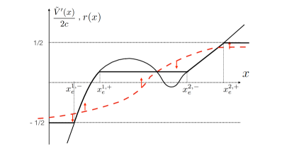
Figure 3: Light black: plot of $\tilde{V}^{\prime}(x)/(2c)$ versus $x$ for a double well potential. Thick black: stationary $r_{\rm stat}(x)$. The support of the density $r^{\prime}_{\rm stat}(x)$ consists of two intervals. Dashed red: initial $r_{0}(x)$. Red arrows indicate the variation of $r(x,t)$ with time $\dot{r}$ has opposite sign to $\dot{x}$. The position of the plateau in $r_{\rm stat}(x)$ is determined by $r_{0}(a)$ where $a$ is the intersection of $r_{0}(x)$ and $\tilde{V}^{\prime}(x)/(2c)$ in the region where the potential is concave.

Multiple wells. For double (or multiple) well types potentials the situation is more involved, since there are regions with $\tilde{V}^{\prime\prime}(x)<0$ where (129) cannot hold. There are thus families of stationary states which depend on the initial condition $r_{0}(x)=r(x,0)$. They consist in a sequence of intervals where (129) holds, separated by empty regions. An example is shown in Fig. 3 for a given initial condition. In that example at large time the support of the density consists of two intervals $[x_{e}^{j,-},x_{e}^{j,+}]$, $j=1,2$. The outer edges are still given by the roots $\tilde{V}^{\prime}(x_{e}^{1,-})=-c$ and $\tilde{V}^{\prime}(x_{e}^{2,+})=-c$. The inner edges $x_{e}^{1,+}$ and $x_{e}^{2,-}$ can be found using the following property. Any point $x=a$ such that $r_{0}(a)=\tilde{V}^{\prime}(a)/2c$ has $\partial_{\tau}r(a,\tau)=0$ hence $r(a,\tau)=r_{0}(a)$ at all times. This is true assuming that $\partial_{x}r(x,\tau)|_{x=a}<+\infty$, which holds for the repulsive case (it fails for the attractive case, see below). The point $x=a$ is a fixed point $\dot{x}=0$ of the flow (128). There are thus two cases

(i) $\tilde{V}^{\prime\prime}(a)-2cr^{\prime}_{0}(a)>0$ in which case $\frac{d\dot{x}}{dx}|_{x=a}<0$ and $x=a$ is an attractive fixed point for the flow (such as $x_{1}$, $x_{3}$ in Fig. 3) which thus belongs to the support of the stationary state.

(ii) $\tilde{V}^{\prime\prime}(a)-2cr^{\prime}_{0}(a)<0$ in which case $\frac{d\dot{x}}{dx}|_{x=a}>0$ and $x=a$ is a repulsive fixed point for the flow. If $\tilde{V}^{\prime\prime}(a)>0$, as for $x_{2}$ in Fig. 1), the point $a$ belongs to the support of the stationary state. However if $\tilde{V}^{\prime\prime}(a)<0$, such as $x_{2}$ in Fig. 3), it cannot belong to the support. Then in the large time limit, $r(x,\tau)$ develops a plateau around the point $x=a$, of value $r_{\infty}(x)=r_{0}(a)=V^{\prime}(a)/(2c)$. This determines uniquely the asymptotic state from the initial condition, within the family of possible stationary states, see Fig. 3. To put it simply, all the particles to the left of $x=a$ end up in the first well, and all those to the right of $a$ end up in the second well.

Note that the sign of $V^{\prime\prime}(a)-2c\partial_{x}r(x,\tau)|_{x=a}$ does not change with time since

$$\partial_{\tau}(V^{\prime\prime}(a)-2c\partial_{x}r(x,\tau)|_{x=a})=-2c\partial_{x}\partial_{\tau}r(x,\tau)|_{x=a}=-2c(V^{\prime\prime}(a)-2c\partial_{x}r(x,\tau)|_{x=a})\partial_{x}r(x,\tau)|_{x=a}$$ (130)

Using (127) and that $(V^{\prime}(a)-2cr(a,\tau))\partial_{x}^{2}r(x,\tau)|_{x=a}=0$ (if we assume $\partial_{x}^{2}r(x,\tau)|_{x=a}<+\infty$ which holds in the repulsive case).

General solution for the dynamics. It is easy to obtain the general solution of (15) by considering $\tau(x,r)$ and using $\frac{\partial_{x}r}{\partial_{\tau}r}=-\partial_{x}\tau$. We obtain $(\tilde{V}^{\prime}(x)-2cr)\partial_{x}\tau=-1$. Let us denote $x_{0}(r)$ the inverse function of the initial condition $r_{0}(x)=r(x,0)$, i.e. $r_{0}(x_{0}(r))=r$. The general solution is then for $r\in[-\frac{1}{2},\frac{1}{2}]$

$$\tau=\int_{x_{0}(r)}^{x}\frac{dy}{2cr-\tilde{V}^{\prime}(y)}$$ (131)

Dynamics without potential. Consider first the system in the absence of external potential, $\tilde{V}(x)=0$. Eq. (131) recovers the perturbative solution of the inviscid Burgers equation

$$2cr\tau=x-x_{0}(r)\quad,\quad r=r_{0}(x-2cr\tau)$$ (132)

equivalently $r(x,\tau)=r_{0}(w(x,\tau))$ where

$$w+2c~{}r_{0}(w)\tau=x\quad\Leftrightarrow\quad w=w(x,\tau)$$ (133)

This solution is valid as long as the map $w\to w+2c~{}r_{0}(w)\tau$ is invertible, i.e. it is valid for all times $\tau$ such that the initial density satisfies

$$1+2c\tau\rho_{0}(x)>0\quad\forall x$$ (134)

In the repulsive case, $c>0$, it is thus valid for all times. Since $\tilde{V}(x)=0$ the particles are expelled to infinity, and for a localized initial condition (132) leads to $r(x,\tau)\simeq\frac{x}{2c\tau}$ for $|x|<2c\tau$ at large $\tau$, a non-stationary solution which has the form of a symmetric front moving at speed $\pm 2c$. An instructive example is to consider a square initial condition $\rho_{0}(x)=\rho(x,0)=\frac{1}{2\ell}\theta(\ell-|x|)$ with $\ell>0$. The exact solution is then

$$r(x,\tau)=\begin{cases}\frac{x}{2(\ell+c\tau)}\quad,\quad|x|<\ell+c\tau\\ \pm 1/2\quad,\quad~{}~{}\,|x|>\ell+c\tau\end{cases}$$ (135)

hence the density remains a square at all times, with a width growing linearly with time

$$\rho(x,\tau)=\frac{1}{2(\ell+c\tau)}\theta(\ell+c\tau-|x|)$$ (136)

i.e. the gas expands ballistically.

In general one can check that the perturbative solution satisfies both that (i) the point $w=a$ such that $r_{0}(a)=0$ is preserved, since at time $\tau$ it corresponds from (133) to $x=a$, hence $r(a,\tau)=r_{0}(a)=0$, and (ii) the center of mass does not move since its position at any time is $\int_{-1/2}^{1/2}drx=\int_{-1/2}^{1/2}dr_{0}(w+2c\tau r_{0})=\int_{-1/2}^{1/2}dr_{0}w$ using that $[r_{0}^{2}]_{-1/2}^{1/2}=0$. Thus the gas expands both such that the number of particle to the left and to the right of $x=a$ remains the same and so that the center of mass of the gas is preserved.

Harmonic well. For the harmonic well, $\tilde{V}^{\prime}(y)=\mu_{0}y$ the solution $r=r(x,\tau)$ from (131) takes the implicit form

$$e^{-\mu_{0}\tau}=\frac{2cr-\mu_{0}x}{2cr-\mu_{0}x_{0}(r)}$$ (137)

Consider for instance the case where all particles start at $x=y$, i.e. $x_{0}(r)=y$. One finds that the density is uniform

$$r(x,\tau)=\frac{\mu_{0}}{2c}\frac{x-ye^{-\mu_{0}\tau}}{1-e^{-\mu_{0}\tau}}~{},~{}\rho(x,\tau)=\frac{\mu_{0}}{2c(1-e^{-\mu_{0}\tau})}$$ (138)

in the time dependent interval $x\in[x_{e}^{-}(\tau),x_{e}^{+}(\tau)]$ with $x_{e}^{\pm}(\tau)=\pm\frac{c}{\mu_{0}}(1-e^{-\mu_{0}\tau})+ye^{-\mu_{0}\tau}$, and zero outside. It converges exponentially fast to the stationary state

$$\rho_{\rm stat}(x)=\begin{cases}\frac{\mu_{0}}{2c}\quad,\quad|x|<\frac{c}{\mu_{0}}\\ 0\quad,\quad|x|>\frac{c}{\mu_{0}}\end{cases}$$ (139)

i.e. a constant density in a finite interval, as was found in the Jellium studies in the regime large $N$ at fixed $c=-\bar{c}$.

Inverse harmonic well. Note that the solution (138) also holds for $\mu_{0}<0$ (concave potential). In that case the gas expands exponentially fast, the two edges being given by $x_{e}^{\pm}(\tau)=(y\pm\frac{c}{|\mu_{0}|})e^{|\mu_{0}|\tau}\mp\frac{c}{\mu_{0}}$. The density inside the interval vanishes exponentially fast $\rho(x,\tau)=\frac{|\mu_{0}|}{2c(e^{|\mu_{0}|\tau}-1)}$ an example of the formation of a plateau in a region with $\tilde{V}^{\prime\prime}(x)<0$, as discussed above.

III.2 Attractive interactions $\bar{c}=-c>0$

In the case of attractive interactions some of the above formula are still valid, but only up to some finite time at which there is formation of delta peaks in the density, which, in the scaling considered here, correspond to packets of particles containing a finite fraction of the $N$ particles. In the context of the Burgers equation for $r(x,t)$ it corresponds to the formation of shocks. In the absence of external potential it corresponds to the string solutions of the LL model.

Consider the case $\tilde{V}(x)=0$. The simplest example is the exact solution (140)

$$\rho(x,\tau)=\frac{1}{2(\ell-\bar{c}\tau)}\theta(\ell-\bar{c}\tau-|x|)$$ (140)

The gas now contracts ballistically. The density becomes a delta function at $x=0$, i.e. $r(x,\tau)$ develops a jump (i.e. a shock) of unit amplitude at $x=0$, in a finite time $\tau=\ell/\bar{c}$.

In fact the solution (140) is very special, as the final position of the shock is its ”naive” position. This is given by arguments similar to those of the previous subsection, i.e. it is the attractive point of the dynamics (128), equal to the root $x=a$ of $-\dot{x}\equiv\tilde{V}^{\prime}(x)+2\bar{c}r_{0}(x)=0$, in that case $a=0$ (since $\tilde{V}(x)=0$).

More generally, when $\rho(x,0)$ is not uniform, the perturbative solution of the Burgers equation (132), (133) breaks down before, and from (134), a shock appears at time

$$\tau=\tau_{s}=\frac{1}{2\bar{c}\max_{x}\rho(x,0)}$$ (141)

and at position $x=x_{s}={\rm argmax}\rho(x,0)$, the location of the maximum of the density. The dynamics beyond that time is more complex (especially in presence of a potential) and one cannot use the above ”naive” argument to predict the position of the shock at large time. This argument to predict the final state works only in the repulsive case, when the perturbative solution holds for all times.

To describe fully the dynamics in the case of attractive interactions, including shocks, one must give a more precise meaning to the inviscid Burgers equation (127) allowing for shocks. This is a standard problem, and the solution can be deduced from the inclusion of the (very small) neglected diffusion term. Anticipating on the study of this term in the next section (note that the noise term remains subdominant as compared to the diffusion term), the proper solution in the case $\tilde{V}(x)=0$ to which we restrict here, is

$$r(x,\tau)=\frac{w(x,\tau)-x}{2\tau\bar{c}}=r(w(x,\tau),0)$$ (142)

$$w(x,\tau):={\rm argmin}_{w\in\mathbb{R}}[E_{x,\tau}(w)]\quad,\quad E_{x,\tau}(w)=\frac{(w-x)^{2}}{4\tau}-\bar{c}\int_{0}^{w}dx^{\prime}r_{0}(x^{\prime})$$ (143)

This formula is valid for any sign of $c=-\bar{c}$. It recovers the perturbative solution of Burgers equation when there is a single minimum in (143), which holds for all times in the repulsive case (since $E_{x,\tau}(w)$ is convex in that case). In the attractive case, the potential energy $-\bar{c}\int_{0}^{w}dx^{\prime}r_{0}(x^{\prime})$ is a concave function with linear behavior at infinity, $\simeq\frac{\bar{c}}{2}|w|$. Beyond the time $\tau=\tau_{s}$, $E_{x,\tau}(w)$ has a (time dependent) number $n+1$ of local minima $w_{i}=w_{i}(x,\tau)$, $w_{1}<\dots<w_{n}$, solutions of

$$\frac{w_{i}-x}{2\bar{c}\tau}=r_{0}(w_{i})$$ (144)

and $n$ maxima (each between two minima). For any given $\tau$ and $x$ the global minimum belongs to this set, $w(x,\tau)={\rm argmin}_{w\in\{w_{i}\}}E_{x,\tau}(w)$. As $x$ is increased (at fixed $\tau$) the global minimum $w(x,\tau)$ takes increasing values in a subset of $p\leq n$ elements $w_{i_{1}}<\dots<w_{i_{p}}$ of $\{w_{i}\}$. This corresponds to $p$ shocks, i.e. $p$ packets of particules being present at time $\tau$. The positions of the shocks $x_{s}^{j}=x_{s}^{j}(\tau)$, $x_{s}^{1}(\tau)<\dots x_{s}^{p}(\tau)$, are determined by the energy degeneracy condition

$$E_{x_{s}^{j},\tau}(w_{i_{j}})=E_{x_{s}^{j},\tau}(w_{i_{j+1}})$$ (145)

One has $p\leq n$ because some of the (higher up, small scale) local minima $w_{i}$ never become the global minimum as $x$ is varied. Accordingly, as $\tau$ increases, the positions of two neighboring shocks may coincide, in which case they merge (i.e. the two delta packets of particles merge), and the intermediate local minima drops from the list.

A simple graphical construction allows to determine these positions according to the ”equal area law”, see Fig. 4, which is a simple consequence of the degeneracy condition (145).

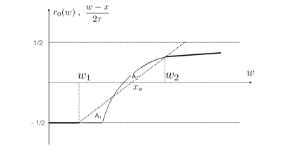
Figure 4: Graphical construction of the solution (143). Light black: plot of the initial condition $r_{0}(w)$ versus $w$. Dashed line: plot of $(w-x)/(2\tau)$ i.e. a straight line of slope $1/(2\tau)$ which intercepts the $w$ axis at $x$. It then intercepts the graph of $r_{0}(w)$ at $w(x,\tau)$ the minimizer of (143). For some values of $x$ there are three intersections, corresponding to two minima of (143) and a maximum. The position of the shock $x=x_{s}$ is attained when the areas $A_{1}$ and $A_{2}$ are equal. Thick black line: resulting value of $r(x,\tau)=r_{0}(w)$ obtained for $w(x,\tau)<w(x^{-},\tau)=w_{1}$ and for $w(x,\tau)>w(x^{-},\tau)=w_{2}$, which exhibits a jump at $x=x_{s}$

At intermediate time there can be a single or several shocks, i.e. delta packets of particles, on top a a smooth density background. In the large time limit they merge and it always remain only a single shock, i.e. a single delta packet containing all the particles, associated to the jump from the leftmost minimum $w_{1}$ to the rightmost minimum $w_{n}$. To investigate the late time dynamics let us rewrite the potential in a form convenient for the large $|w|$ asymptotics

$$\int_{0}^{w}dx^{\prime}r_{0}(x^{\prime})=\frac{w}{2}-\kappa_{+}-g_{+}(w)=-\frac{w}{2}+\kappa_{-}+g_{-}(w)\quad,\quad r_{0}(w)=\frac{1}{2}-g^{\prime}_{+}(w)=-\frac{1}{2}+g^{\prime}_{-}(w)$$ (146)

where the function $g_{+}(w)$ decays to zero as $w\to+\infty$, and $g_{-}(w)$ decays to zero as $w\to-\infty$. From the local minima condition (144) we obtain

$$w_{1}=x-\bar{c}\tau+2\bar{c}\tau g^{\prime}_{-}(w_{1})\quad,\quad w_{n}=x+\bar{c}\tau-2\bar{c}\tau g^{\prime}_{+}(w_{n})$$ (147)

since $w_{1}\to-\infty$ and $w_{n}\to+\infty$ as $\tau\to+\infty$. The shock position $x_{s}$ is determined by $E_{x_{s},\tau}(w_{1})=E_{x_{s},\tau}(w_{n})$ which yields using (144)

$$\bar{c}^{2}\tau(r_{0}(w_{n})^{2}-r_{0}(w_{1})^{2})-\bar{c}\int_{w_{1}}^{w_{n}}dx^{\prime}r_{0}(x^{\prime})=0$$ (148)

which, using (146) and its derivative, leads to

$$\bar{c}\tau(g^{\prime}_{-}(w_{1})-g^{\prime}_{+}(w_{n}))(1-g^{\prime}_{-}(w_{1})-g^{\prime}_{+}(w_{n}))=\frac{w_{1}+w_{n}}{2}-\kappa_{+}-\kappa_{-}-g_{+}(w_{n})-g_{+}(w_{1})$$ (149)

We now insert (147) and after some simplifications we obtain the shock position as

$$x_{s}=\kappa_{+}+\kappa_{-}+g_{+}(w_{n})+g_{+}(w_{1})+\bar{c}\tau(g^{\prime}_{+}(w_{n})^{2}-g^{\prime}_{-}(w_{1})^{2})$$ (150)

Until now this is exact as long as there is only one shock. It can also be written as

$$x_{s}=-\int_{w_{1}}^{w_{n}}dx^{\prime}(r_{0}(x^{\prime})-\frac{1}{2}{\rm sgn}(x^{\prime}))+\bar{c}\tau((r_{0}(w_{n})-\frac{1}{2})^{2}-(r_{0}(w_{1})+\frac{1}{2})^{2})$$ (151)

which is again exact and only assumes a single shock with $w_{1}<0$ and $w_{n}>0$. Inserting the large $\tau$ asymptotics we find $x_{s}(\tau)=x_{s}(+\infty)+\delta x_{s}(\tau)$ where the final position is simply given by the initial center of mass position

$$x_{s}(\infty)=\kappa_{+}+\kappa_{-}=-\int_{-\infty}^{+\infty}(r_{0}(x^{\prime})-\frac{1}{2}{\rm sgn}(x^{\prime}))=\int_{-\infty}^{+\infty}dxx\,\rho(x,0)$$ (152)

and the convergence towards that position can be estimated as

$$\delta x(\tau)\simeq g_{+}(\bar{c}\tau)+g_{-}(-\bar{c}\tau)+\bar{c}\tau(g^{\prime}_{+}(\bar{c}\tau)^{2}-g^{\prime}_{-}(-\bar{c}\tau)^{2})$$ (153)

Similarly the fraction of particles in the shock converges to unity as

$$r_{0}(w_{n})-r_{0}(w_{1})=1-g^{\prime}_{+}(w_{n})-g^{\prime}_{-}(w_{1})\simeq 1-g^{\prime}_{+}(\bar{c}\tau)-g^{\prime}_{-}(-\bar{c}\tau)$$ (154)

We have assumed that $r_{0}(x)-\frac{1}{2}{\rm sgn}(x)$ converges to zero faster than $1/|x|$ at large $|x|$, equivalently that the center of mass position can be defined. Note that the fact that the center of mass position is independent of time when $V(x)=0$ and upon neglecting the noise is easily seen by multiplying (11) by $x$, integrating over $x$ and using integrations by part.

IV Large $N$ with $c=\gamma/N$

We consider now the large $N$ limit with $\gamma=Nc$ fixed, and we also note $\bar{\gamma}=N\bar{c}=-\gamma$. This scaling allows to study in more details the attractive case and the structure of the shocks. Here one does not rescale time, nor the potential $V(x)$. One sees that in (13) one can still neglect the noise term, but now one must keep the diffusion term, and one obtains ($\gamma$ has arbitrary sign here) the evolution equation of $r(x,t)$ as

$$\partial_{t}r=T\partial_{x}^{2}r+2\bar{\gamma}~{}r\partial_{x}r+V^{\prime}(x)\partial_{x}r$$ (155)

where $\gamma$ has arbitrary sign.

IV.1 No external potential

Consider first $V(x)=0$. We will look for a solution for $r(x,t)$ in the form

$$r(x,t)=\frac{T}{\bar{\gamma}}\partial_{x}\log Z(x,t)$$ (156)

where $Z(x,t)$ is the solution of the heat equation

$$\partial_{t}Z(x,t)=T\partial^{2}_{x}Z(x,t)$$ (157)

From (156), we must choose the initial condition to be $Z(x,t=0)=e^{\frac{\bar{\gamma}}{T}\int_{a}^{x}dx^{\prime}r_{0}(x^{\prime})}$. Here $a$ is arbitrary and we will choose $a=0$ for convenience. Given this initial condition, if $Z(x,t)$ obeys (157) then $H(x,t)=\log Z(x,t)$ obeys $\partial_{t}H=T\partial_{x}^{2}H+T(\partial_{x}H)^{2}$ and, taking a derivative, $r=\frac{T}{\bar{\gamma}}\partial_{x}H$ satisfies the Burgers equation (162) (with $V(x)=0$), with the proper initial condition. Since the solution for $Z(x,t)$ is

$$Z(x,t)=\int\frac{dw}{\sqrt{4\pi Tt}}e^{-\frac{(w-x)^{2}}{4Tt}+\frac{\bar{\gamma}}{T}\int_{0}^{w}dx^{\prime}r_{0}(x^{\prime})}$$ (158)

it implies, using (156), that the solution for $r(x,t)$ is

$$r(x,t)=\frac{\int\frac{dw}{\sqrt{4\pi Tt}}\frac{w-x}{2\bar{\gamma}t}e^{-\frac{(w-x)^{2}}{4Tt}+\frac{\bar{\gamma}}{T}\int_{0}^{w}dx^{\prime}r(x^{\prime},0)}}{\int\frac{dw}{\sqrt{4\pi Tt}}e^{-\frac{(w-x)^{2}}{4Tt}+\frac{\bar{\gamma}}{T}\int_{0}^{w}dx^{\prime}r(x^{\prime},0)}}$$ (159)

Note that this solution is valid irrespective of the sign of $\bar{\gamma}=-\gamma$.

One can recover the results of Section III in the fixed $\bar{c}$ large $N$ limit. To this aim one sets $t=\tau/N$ and $\bar{\gamma}=N\bar{c}$ and take $N\to+\infty$ in (159). The argument of the exponential is then uniformly of $O(N)$ and from the saddle point method the integral is dominated by the maximum of the integrand. One then recovers the solution of the inviscid Burgers equation given above in (143).

Attractive interactions $\bar{\gamma}>0$

Thus, in the large $N$ limit with fixed $\bar{\gamma}=N\bar{c}$, if we take $\bar{\gamma}/T$ of $O(1)$ but large, there is a smooth crossover to the results of the previous section. At finite $\bar{\gamma}>0$ the shocks have a finite width of order $O(T/\bar{\gamma})$ (see below), which vanishes in the limit. So here, by keeping the diffusion term, we are looking at the system on the scale of the shock width. For a localized initial density there is usually a single shock whose amplitude is growing. For a multimodal type distribution there may be several shocks forming which then merge. Each shock contains a finite fraction of the number of particles. At large time there remains a single shock, which we now study.

One easily checks that for $\bar{\gamma}>0$ the following initial condition is stationary, $r_{\rm stat}(x)=r(x,t)=r_{0}(x)$ for all $t$

$$\int^{w}dx^{\prime}r_{\rm stat}(x^{\prime})=\int^{w}dx^{\prime}r_{0}(x^{\prime})=\frac{T}{\bar{\gamma}}\log[\cosh[\frac{1}{2T}\bar{\gamma}(w-x_{s})]]$$ (160)

$$r_{\rm stat}(x)=\frac{1}{2}\tanh(\frac{\bar{\gamma}}{2T}(x-x_{s}))\quad,\quad\rho_{\rm stat}(x)=\frac{\bar{\gamma}}{4T}\frac{1}{\cosh^{2}(\frac{\bar{\gamma}}{2T}(x-x_{s}))}$$ (161)

either by inserting into (159) or by checking that it satisfies

$$T\partial_{x}^{2}r_{\rm stat}(x)+2\bar{\gamma}~{}r_{\rm stat}(x)\partial_{x}r_{\rm stat}(x)=0$$ (162)

It describes a single shock, i.e. a packet containing the $N$ particles.

The stationary distribution is this not unique since $x_{s}$ is arbitrary. The low lying diffusion modes correspond to the diffusion of the center of mass. Indeed it is exact for any $N$ that the center of mass mode $\bar{x}(t)=\frac{1}{N}\sum_{i}x_{i}(t)$ undergoes diffusion, i.e. with ${\rm Var}\bar{x}(t)=\frac{2T}{N}t$ when started from $\bar{x}(t)=0$ at $t=0$. This motion is subdominant in the limit studied here.

Remark. This stationary solution has the same form as the well known soliton of the focusing non-linear Schrödinger equation (NLSE). The NLSE also describes a semi-classical limit of the delta Bose gas.

Convergence to the stationary state: droplet initial condition. Let us study the dynamics with initially all particles at $x=0$, hence $r_{0}(x)=\frac{1}{2}{\rm sgn}(x)$. Inserting into (156), (158) or (159) we obtain

$$r(x,t)=\frac{1}{\bar{\gamma}}\partial_{x}\log\left(e^{\frac{\bar{\gamma}}{2}x}(1+{\rm erf}(\frac{x+\bar{\gamma}t}{2\sqrt{t}}))+e^{-\frac{\bar{\gamma}}{2}x}(1-{\rm erf}(\frac{x-\bar{\gamma}t}{2\sqrt{t}}))\right)$$ (163)

In the large time limit, it converges to $r_{\rm stat}(x)$ given by (160) as

$$r(x,t)\simeq r_{\rm stat}(x)-\frac{e^{-\frac{\bar{\gamma}^{2}}{4}t}}{\bar{\gamma}^{2}\sqrt{\pi t}}\partial_{x}\left(\frac{e^{-\frac{x^{2}}{4t}}}{\cosh(\frac{\bar{\gamma}x}{2})}\right)$$ (164)

This decay rate is compatible with the one predicted by the Lieb-Liniger model, $\simeq\frac{N^{2}\bar{c}^{2}}{4}=\frac{\bar{\gamma}^{2}}{4}$ at large $N$, as expected since the initial condition is very localized.

Convergence to the stationary state: slow decaying solutions. Consider now the following initial condition with two packets of particles centered at positions $x_{1}$ and $x_{2}$ (in the remainder of this subsection we set $T=1$ for notational simplicity)

$$\int^{w}dx^{\prime}r_{0}(x^{\prime})=\frac{1}{\bar{\gamma}}\log[\cosh[\frac{p_{1}\bar{\gamma}}{2}(w-x_{1})]+\frac{1}{\bar{\gamma}}\log[\cosh[\frac{p_{2}\bar{\gamma}}{2}(w-x_{2})]]\quad,\quad p_{1}+p_{2}=1$$ (165)

$$r_{0}(x)=\frac{p_{1}}{2}\tanh(\frac{p_{1}\bar{\gamma}}{2}(x-x_{1}))+\frac{p_{2}}{2}\tanh(\frac{p_{2}\bar{\gamma}}{2}(x-x_{2}))$$ (166)

which has the proper boundary conditions $r_{0}(x)=\pm\frac{1}{2}$ at $x\to\pm\infty$. If the packets are well separated one can consider that they contain respectively the fractions $p_{1}$ and $p_{2}$ of particles with $p_{1}+p_{2}=1$. Inserting (165) into (158) and (159) one finds

$$r(x,t)=\frac{1}{\bar{\gamma}}\partial_{x}\log\left(\cosh(\frac{\bar{\gamma}}{2}(x-x_{s}))+e^{-p_{1}p_{2}\bar{\gamma}^{2}t}\cosh(\frac{\bar{\gamma}}{2}((p_{1}-p_{2})x-(p_{1}x_{1}-p_{2}x_{2})))\right)$$ (167)

which converges at large time to the stationary solution (160), i.e to a single shock containing all the particles at position

$$x_{s}=p_{1}x_{1}+p_{2}x_{2}$$ (168)

At finite time this solution describes two coalescing shocks. Note that the decay rate $1/t_{2}$ is

$$1/t_{2}=p_{1}(1-p_{1})\bar{c}^{2}N^{2}\leq\frac{1}{4}\bar{c}^{2}N^{2}$$ (169)

i.e. the decay is slower than the one predicted by the gap in the LL bosonic spectrum between the ground state and the one particle excitation. As explained in the text, this is because the spatial decay of the initial density, here $\rho_{0}(x)\sim e^{-\min(p_{1},p_{2})N\bar{c}|x|}$ at large $x$ is slower than the one of $\Psi_{0}(\vec{x}=(x,0,\dots,0))\sim e^{-\frac{N-1}{2}\bar{c}|x|}$.

When the packets are well separated (as compared to their widths), one can describe their finite time dynamics by considering piecewise superpositions of elementary solutions interpolating between $a_{j}-\frac{p_{j}}{2}$ and $a_{j}+\frac{p_{j}}{2}$ of the form

$$r(x,t)=a_{j}+\frac{p_{j}}{2}\tanh(\frac{p_{j}}{2}\bar{\gamma}(x-x_{j}+2a_{j}\gamma t))$$ (170)

with $a_{j}=-\frac{1}{2}+p_{1}+\dots+p_{j-1}$. The center of each packet then moves balistically as $x_{s}=x_{j}-2a_{j}\gamma t$. This solution is a good approximation until the packets get closer together.

Dynamics for repulsive interactions $\gamma>0$

To obtain some insight into the Burgers dynamics for the expanding gas (repulsive case) we can either study the solution (163) setting $\bar{\gamma}=-\gamma$ with $\gamma>0$, or study again the case of the square initial condition $\rho(x,0)=\frac{1}{2\ell}\theta(\ell-|x|)$ with $a>0$, which was solved in (135) and (140) in the fixed $\bar{c}$ large $N$ limit (inviscid limit). Inserting into (159) we obtain

$$r(x,t)=-\frac{1}{\gamma}\partial_{x}\log\left(f(x,t)+f(-x,t)\right)$$ (171)

$$f(x,t)=\frac{e^{-\frac{\gamma x^{2}}{4({\ell}+\gamma t)}}}{\sqrt{1+\frac{\gamma t}{{\ell}}}}\text{erf}\left(\frac{{\ell}+\gamma t+x}{2\sqrt{t}\sqrt{1+\frac{\gamma t}{{\ell}}}}\right)+e^{\frac{1}{4}\gamma({\ell}+\gamma t+2x)}\text{erfc}\left(\frac{{\ell}+\gamma t+x}{2\sqrt{t}}\right)$$ (172)

These solutions look like (140) but with a smoothed boundary.

IV.2 Harmonic potential, repulsive interactions

Consider the harmonic well $V(x)=\mu\frac{x^{2}}{2}$ with $\mu>0$. In the simplest case of no interactions $\gamma=0$ the stationary solution is simply

$$r_{\rm stat}(x)=\frac{1}{2}{\rm Erf}(\frac{x\sqrt{\mu}}{\sqrt{2T}})\quad,\quad\rho_{\rm stat}(x)=\frac{\sqrt{\mu}}{\sqrt{2\pi T}}e^{-\frac{\mu x^{2}}{2T}}$$ (173)

Consider now repulsive interactions $\gamma>0$. Defining $r(x,t)=\frac{\mu}{2\gamma}x+\tilde{r}(x,t)$ (so that $\tilde{r}(x,t)=0$ in the stationary state in the absence of the second derivative) one can rewrite (162) as

$$\partial_{t}\tilde{r}=T\partial_{x}^{2}\tilde{r}-2\gamma\tilde{r}\partial_{x}\tilde{r}-\mu\tilde{r}$$ (174)

which is the Burgers equation with friction $\mu$ for $\tilde{r}(x,t)$.

Let us search for the stationary solution $\partial_{t}\tilde{r}=0$ of (174), which we call $\tilde{r}_{\rm stat}$. It is easy to see that $\tilde{r}_{\rm stat}$ takes the scaling form $\tilde{r}_{\rm stat}(x)=-\frac{\sqrt{\mu T}}{2\gamma}R(x\sqrt{\frac{\mu}{T}})$, hence $r_{\rm stat}(x)$ is of the form

$$r_{\rm stat}(x)=\frac{\sqrt{\mu T}}{2\gamma}\hat{r}_{g}(x\sqrt{\frac{\mu}{T}})\quad,\quad\hat{r}_{g}(y)=y-R_{g}(y)\quad,\quad\rho_{\rm stat}(x)=\frac{\mu}{2\gamma}\hat{\rho}_{g}(x\sqrt{\frac{\mu}{T}})\quad,\quad\hat{\rho}_{g}(y)=1-R_{g}^{\prime}(y)$$ (175)

where we have introduced the dimensionless parameter

$$g=\frac{\gamma}{\sqrt{\mu T}}$$ (176)

The scaling functions form a one parameter family depending on the parameter $g$. The function $R(y)=R_{g}(y)$ is a dimensionless function solution of

$$0=R^{\prime\prime}(y)+R(y)R^{\prime}(y)-R(y)$$ (177)

which amounts to set $\mu=1$, $\gamma=1/2$ and $T=1$. Since $r(\pm\infty)=\pm\frac{1}{2}$, hence $R_{g}(y)$ must satisfy for $y\to\pm\infty$

$$R(y)\simeq y\mp g$$ (178)

and we expect $R_{g}(y)$ to be an odd function. The condition (178) can be equivalently written as

$$\int_{-\infty}^{+\infty}dy(1-R^{\prime}(y))=2g$$ (179)

which will be useful below.

The equation (177) is an autonomous equation, $y$ does not appear. The usual method is to write $R^{\prime}(y)=w(R(y))$ for some function $w(R)$ of $R$. Then $R^{\prime\prime}(y)=w(R(y))w^{\prime}(R(y))$ and the equation (177) becomes an equation for $w(R)$ where now $R$ is the variable

$$ww^{\prime}=R(1-w)\quad\Rightarrow\quad\frac{wdw}{1-w}=RdR$$ (180)

This can be integrated as

$$w+\log(1-w)=-\frac{1}{2}R^{2}-b$$ (181)

where $b$ is a constant as yet undetermined. Clearly $y\to\pm\infty$ corresponds to $R\to\pm\infty$ and to $w\to 1^{-}$.

There are several equivalent ways to write the solution. The first one is to solve (181) for $w(R)$ as

$$w=1+W(-e^{-b-1-\frac{R^{2}}{2}})$$ (182)

where here $W(z)=\sum_{n\geq 1}\frac{(-n)^{n-1}}{n!}z^{n}$ is the first branch of the Lambert function solution of $z=We^{W}$, with $z\in[e^{-1},+\infty[$ and $W(e^{-1})=-1$. The condition (179) implies that

$$\int_{-\infty}^{+\infty}(1-w)dx=\int_{-\infty}^{+\infty}\frac{1-w(R)}{w(R)}dR=2g$$ (183)

which allows to determine the constant $b=b_{g}>0$ as a function of $g$ as the solution of

$$\int_{0}^{+\infty}du\,\left(\frac{1}{1+W(-e^{-b-1-\frac{u^{2}}{2}})}-1\right)=g$$ (184)

Finally since $\frac{dy}{dR}=\frac{1}{w(R)}$ one obtains that $R(y)=R_{g}(y)$ is determined by inverting from

$$\int_{0}^{R}\frac{du}{1+W(-e^{-b-1-\frac{u^{2}}{2}})}=y$$ (185)

with $b=b_{g}$. The scaling function of the density is then determined parametrically by eliminating $R$ between (185) and

$$\hat{\rho}(y)=-W(-e^{-b-1-\frac{R^{2}}{2}})$$ (186)

Thus the density depends on the parameter $b=b_{g}$ which depends on $g$ via (184).

In the limit $g\ll 1$ one has $b\to+\infty$ and one can expand $W(z)$ at small $z$. From (184) one obtains

$$z=e^{-b-1}=\sqrt{\frac{2}{\pi}}g-\frac{2\sqrt{2}g^{2}}{\pi}+\frac{\left(8\sqrt{2}-3\sqrt{6}\right)g^{3}}{\pi^{3/2}}+O\left(g^{5}\right)$$ (187)

Next one obtains

$$R_{g}(y)=y-g\,\text{erf}\left(\frac{y}{\sqrt{2}}\right)+\frac{g^{2}\left(\left(\sqrt{2}e^{-\frac{y^{2}}{2}}+2\right)\text{erf}\left(\frac{y}{\sqrt{2}}\right)-2\text{erf}(y)\right)}{\sqrt{\pi}}+O\left(g^{3}\right)$$ (188)

and finally

$$\hat{\rho}(y)=\sqrt{\frac{2}{\pi}}ge^{-\frac{y^{2}}{2}}+\frac{g^{2}e^{-y^{2}}\left(\sqrt{2\pi}e^{\frac{y^{2}}{2}}y\text{erf}\left(\frac{y}{\sqrt{2}}\right)-2\sqrt{2}e^{\frac{y^{2}}{2}}+2\right)}{\pi}+O\left(g^{3}\right)$$ (189)

The leading term recovers the result (173) for $\gamma=0$

In the other limit $g\gg 1$ one finds that in the variable $u=y/g$ the density goes to a square function

$$\hat{\rho}(y)\simeq\theta(1-\frac{|y|}{g})\quad,\quad\rho(x)\simeq\frac{\mu}{2\gamma}\theta(1-\frac{|x|\mu}{\gamma})$$ (190)

Since in that limit $b\to 0$, one can check that indeed $\hat{\rho}(0)\to 1$ since

$$W(-e^{-1-b})=-1+\sqrt{2b}-\frac{2}{3}b+\dots$$ (191)

Alternative method. To solve the equation one can write instead, starting from (181)

$$R(y)=F(w)\quad,\quad F(w)=\pm\sqrt{-2b-2(w+\log(1-w))}$$ (192)

From the definition $w=R^{\prime}(x)$ one has

$$dx=\frac{dR}{w}=\frac{F^{\prime}(w)dw}{w}$$ (193)

This leads to the solution in parametric form

$$R=F(w)=\pm\sqrt{-2b-2(w+\log(1-w))}=\pm\sqrt{2}\sqrt{-1-b+e^{z}-z}$$ (194)

$$y=\int^{w}\frac{F^{\prime}(u)du}{u}=\pm\int^{w}\frac{du}{\sqrt{2}(1-u)\sqrt{-b-u-\log(1-u)}}=\pm\int_{z}\frac{dz}{\sqrt{2}\sqrt{-b-1+e^{z}-z}}$$ (195)

defining $1-w=e^{z}$.

Remark. Similar looking equations appear in a problem of self-gravitating gas Kumar2017 , but with somewhat different interactions, which are linear and attractive at small scale and quadratic and repulsive at large scales (and there is no external quadratic well).

V Coulomb gas

Here we discuss the Coulomb gas formulation, which also allows to determine the stationary state in the large $N$ limit.

The (exact) Dean-Kawasaki equation (11) for the RD system in terms of the density field $\tilde{\rho}(x,t)=\sum_{i}\delta(x-x_{i}(t)))$ normalized to $N$, and restoring the temperature $T$, reads

$$\partial_{t}\tilde{\rho}(x,t)=T\partial_{x}^{2}\tilde{\rho}(x,t)+\partial_{x}[\sqrt{2T\tilde{\rho}(x,t)}\eta(x,t)]+\partial_{x}[V^{\prime}(x)\tilde{\rho}(x,t)+\bar{c}\tilde{\rho}(x,t)\int dy\tilde{\rho}(y,t){\rm sgn}(x-y))]$$ (196)

where $\eta(x,t)$ is a unit space time white noise. Following Dean ; DeanPrivate it can be rewritten as an explicit equilibrium dynamics

$$\partial_{t}\tilde{\rho}(x,t)=-\int dyR(x,y;\tilde{\rho}(.,t))\frac{\delta H[\tilde{\rho}(.,t)]}{\delta\tilde{\rho}(y,t)}+\xi(x,t)\quad,\quad\langle\xi(x,t)\xi(y,t)\rangle=2TR(x,y;\tilde{\rho}(.,t))\delta(t-t^{\prime})$$ (197)

where

$$R(x,y;\tilde{\rho})=\partial_{x}\partial_{y}(\sqrt{\tilde{\rho}(x)\tilde{\rho}(y)}\delta(x-y))=\partial_{x}(\tilde{\rho}(x,t)\partial_{y}\delta(x-y))$$ (198)

and the energy functional is

$$H[\tilde{\rho}]=\int dxV(x)\tilde{\rho}(x)+\frac{\bar{c}}{2}\int dxdx^{\prime}|x-x^{\prime}|\tilde{\rho}(x)\tilde{\rho}(x^{\prime})+T\int dx\tilde{\rho}(x)\log\tilde{\rho}(x)$$ (199)

The last term is the so-called entropy term. Indeed one has

$$\frac{\delta H[\tilde{\rho}]}{\delta\tilde{\rho}(y)}=V(y)+\bar{c}\int dx^{\prime}|y-x^{\prime}|\tilde{\rho}(x^{\prime})+T(1+\log\tilde{\rho}(y))$$ (200)

Using that for any function $f(y)$, upon integration by part,

$$-\int dyR(x,y;\tilde{\rho})f(y)=-\int dy\partial_{x}(\tilde{\rho}(x)\partial_{y}\delta(x-y))f(y)=\partial_{x}(\tilde{\rho}(x)f^{\prime}(x))$$ (201)

one sees that (197) is equivalent to (196).

Thus the stochastic dynamics of the system satisfies detailed balance, and generically converges to the equilibrium measure

$${\cal P}_{\rm stat}[\tilde{\rho}]\propto\exp\left(-\frac{H[\tilde{\rho}]}{T}\right)$$ (202)

whenever the latter is well defined. Note that it does not say how fast this convergence holds. It thus describes the limit where time is taken to infinity first.

Let us now consider the two large $N$ limits studied here.

V.1 Large $N$ at fixed $c=-\bar{c}$, $V(x)=N\tilde{V}(x)$

Let define, as in the text, $\rho(x,t)=\frac{1}{N}\tilde{\rho}(x,t)=\frac{1}{N}\sum_{i}\delta(x-x_{i}(t)))$ the density normalized to unity. In this regime we consider large $N$ at fixed $c=-\bar{c}$, and scale the potential as $V(x)=N\tilde{V}(x)$ with fixed $\tilde{V}(x)$. The energy becomes

$$H[\tilde{\rho}]=N^{2}{\cal E}[\rho]+O(N)\quad,\quad{\cal E}[\rho]=-\frac{c}{2}\int dxdx^{\prime}|x-x^{\prime}|\rho(x)\rho(x^{\prime})+\int dx\tilde{V}(x)\rho(x)$$ (203)

where we can neglect the entropy term in that regime since it is $O(N)$. The equilibrium measure $P_{\rm stat}\propto e^{-N^{2}{\cal E}[\rho]/T}$, is dominated by the energy minimum. To minimize under the constraint $\int dx\rho(x)=1$ one adds the Lagrange multiplier term $\nu(\int dx\rho(x)-1)$ to ${\cal E}[\rho]$. The saddle point equation gives

$$\frac{\delta{\cal E}}{\delta\rho(x)}=-c\int dx^{\prime}|x-x^{\prime}|\rho(x^{\prime})+\tilde{V}(x)+\nu=0$$ (204)

for any $x$ in the support of $\rho(x)$. Taking a derivative we find that either $\rho(x)=0$ or

$$\partial_{x}\frac{\delta{\cal E}}{\delta\rho(x)}=-c\int dx^{\prime}{\rm sgn}(x-x^{\prime})\rho(x^{\prime})+\tilde{V}^{\prime}(x)=-2c\,r(x)+\tilde{V}^{\prime}(x)=0$$ (205)

where we used that $\int dx^{\prime}{\rm sgn}(x-x^{\prime})\rho(x^{\prime})=2r(x)$. Hence we find that for any point $x$ inside the support of the density one has $r(x)=\tilde{V}^{\prime}(x)/(2c)$ and $\rho(x)=\tilde{V}^{\prime\prime}(x)/(2c)$ (and, since $-1/2\leq r(x)\leq 1/2$, any point such that $\tilde{V}^{\prime}(x)>c$ cannot belong to the support). This coincides with the result (129) which was obtained by considering the large time limit for $c>0$ (the limit $N\to\infty$ being taken first). There we gave a complete discussion of the determination of the support for various types of potentials $\tilde{V}(x)$. We would like to know how it compares with the Coulomb gas formulation. Let us note that the minimum energy verifies, using (217)

$${\cal E}_{\rm min}=\int dx\tilde{V}(x)\rho(x)-\frac{1}{2}\nu$$ (206)

Let us check whether (217) is verified. Suppose that the support is a union of (ordered) intervals $[a_{i},b_{i}]$. Each interval contributes to the first term in the RHS of (217) as

$$-c\int_{a_{i}}^{b_{i}}dx^{\prime}|x-x^{\prime}|\rho(x^{\prime})=-\frac{1}{2}\int_{a_{i}}^{b_{i}}dx^{\prime}|x-x^{\prime}|\tilde{V}^{\prime\prime}(x^{\prime})=\frac{1}{2}\int_{a_{i}}^{b_{i}}dx^{\prime}{\rm sgn}(x^{\prime}-x)\tilde{V}^{\prime}(x^{\prime})-\frac{1}{2}[|x-x^{\prime}|\tilde{V}^{\prime}(x^{\prime})]_{a_{i}}^{b_{i}}$$ (207)

$$=-\int_{a_{i}}^{b_{i}}dx^{\prime}\delta(x-x^{\prime})\tilde{V}(x^{\prime})+\frac{1}{2}[{\rm sgn}(x^{\prime}-x)\tilde{V}(x^{\prime})]_{a_{i}}^{b_{i}}-\frac{1}{2}[|x-x^{\prime}|\tilde{V}^{\prime}(x^{\prime})]_{a_{i}}^{b_{i}}$$ (208)

If $x$ belongs to one of the interval, then (217) holds provided the following sum is a constant in $x$

$$\sum_{i}\frac{1}{2}[{\rm sgn}(x^{\prime}-x)\tilde{V}(x^{\prime})]_{a_{i}}^{b_{i}}-\frac{1}{2}\sum_{i}[|x-x^{\prime}|\tilde{V}^{\prime}(x^{\prime})]_{a_{i}}^{b_{i}}=-\nu$$ (209)

Let us examine several cases

Single interval. Consider first the case where the support is a single interval $[a_{1},b_{1}]$, which is the case for convex potentials, as in Fig. 1 (with $a_{1}=x_{e}^{-}$ and $b_{1}=x_{e}^{+}$). In that case we know that $\tilde{V}^{\prime}(a_{1})=-c$ and $\tilde{V}^{\prime}(b_{1})=c$. The first term gives $\frac{1}{2}(\tilde{V}(b_{i})+\tilde{V}(a_{i}))$ and the second $-\frac{c}{2}(b_{i}-a_{i})$, which are constants. Hence (217) is verified with $\nu=-\frac{1}{2}(\tilde{V}(b_{i})+\tilde{V}(a_{i}))+\frac{c}{2}(b_{i}-a_{i})$ and the energy at the minimum is then

$${\cal E}_{\rm min}=\frac{1}{2c}\int_{a_{1}}^{b_{1}}dx\tilde{V}(x)\tilde{V}^{\prime\prime}(x)+\frac{1}{4}(\tilde{V}(b_{i})+\tilde{V}(a_{i}))-\frac{c}{4}(b_{i}-a_{i})$$ (210)

In the case of the quadratic potential one finds ${\cal E}_{\rm min}=-\frac{1}{6}c^{2}/\mu_{0}$.

Two intervals. Consider now the case where the support consists in two intervals, as is the case for the double well potential, as represented in Fig. 3 with $a_{i}=x_{e}^{i,-}$ and $b_{i}=x_{e}^{i,+}$. We have (see the figure)

$$\tilde{V}^{\prime}(a_{1})=-c\quad,\quad\tilde{V}^{\prime}(b_{2})=+c\quad,\quad\tilde{V}^{\prime}(a_{2})=\tilde{V}^{\prime}(b_{1})$$ (211)

which implies the normalisation $\int dx\rho(x)=\frac{1}{2c}(\int_{a_{1}}^{b_{1}}\tilde{V}^{\prime\prime}(x)+\int_{a_{2}}^{b_{2}}\tilde{V}^{\prime\prime}(x))=1$. We obtain the two terms in (209)

$$-\nu_{\pm}:=\frac{1}{2}(\pm\tilde{V}(b_{1})+\tilde{V}(a_{1})+\tilde{V}(b_{2})\mp\tilde{V}(a_{2}))-\frac{1}{2}(\pm b_{1}\tilde{V}^{\prime}(b_{1})+a_{1}\tilde{V}^{\prime}(a_{1})+b_{2}\tilde{V}^{\prime}(b_{2})\mp a_{2}\tilde{V}^{\prime}(a_{2}))=-\nu$$ (212)

where the plus sign is for $x$ in the first interval and the $-$ sign in the second. Note that the term linear in $x$ cancels using (211). In the dynamics we found that the height of the plateau in the rank field, $r(b_{1})=\frac{\tilde{V}^{\prime}(b_{1})}{2c}=r(a_{2})=\frac{\tilde{V}^{\prime}(b_{2})}{2c}$, was determined by the initial condition. Here we see that for both signs in (212) to give the same (i.e. compatible) result, we need in addition to (211)

$$\tilde{V}(b_{1})-b_{1}\tilde{V}^{\prime}(b_{1})=\tilde{V}(a_{2})-a_{2}\tilde{V}^{\prime}(a_{2})$$ (213)

These two conditions can also be written as

$$\int_{a_{2}}^{b_{1}}dx\,\tilde{V}^{\prime\prime}(x)=0\quad,\quad\int_{a_{2}}^{b_{1}}dx\,x\tilde{V}^{\prime\prime}(x)=0$$ (214)

which determine the position of the plateau in the Coulomb gas. For instance for a symmetric double well $\tilde{V}(x)=\frac{x^{4}}{12}-\frac{x^{2}}{2}$ we obtain that the plateau is at level $r(b_{1})=r(a_{2})=0$, i.e. $a_{2}=-b_{1}=\sqrt{3}$ (setting $c=1$) with $V^{\prime}(a_{2})=V^{\prime}(b_{1})=0$. We have checked that this indeed realizes the minimum of the energy ${\cal E}(\rho)$ as compared to allowing different levels for the plateau as obtained in the dynamics.

To conclude this subsection, the Coulomb gas gives the equilibrium state of the system, i.e. the infinite time limit is taken first, to obtain the Gibbs measure (202), and only in a second stage the large $N$ limit is performed on this equilibrium state. In the dynamics of Section III we have performed large $N$ first and neglected the noise. In cases such as double well potentials, convergence to the true equilibrium requires some noise to cross barriers. Hence at large $N$ there are two time scales in the dynamics. First a rapid convergence to a metastable state as in Fig. 3, where the number of particles in each well is determined by the initial condition. This stage is captured by the dynamics of Section III. Next, on much larger time scales, particles undergo barrier crossing, so that the ”chemical potentials” $\nu_{\pm}$ in each well become identical, leading to the equilibrium plateau (214). It would be interesting to study that slow dynamics.

Remark. It is interesting to note that one can rewrite the energy (203) using integrations by part in terms of the rank field as

$${\cal E}[\rho]=c\int dx(r(x)-\frac{1}{2}{\rm sgn}(x))^{2}+\int dx\,(c\,{\rm sgn}(x)-\tilde{V}^{\prime}(x))(r(x)-\frac{1}{2}{\rm sgn}(x))$$ (215)

Attractive case $c=-\bar{c}<0$. In that case it is easy to see that the electrostatic energy (which is positive) is minimum by itself (and vanishes) for $\rho(x)=\delta(x-x_{s})$, which correspond to a single shock at position $x_{s}$ containing a unit fraction of the particles. In the absence of a potential $x_{s}$ is arbitrary. In the presence of an external potential, the potential energy will be minimized (also by itself) if $x_{s}$ is chosen at the minimum of this potential (assuming that there is one unique such minimum).

V.2 Large $N$ at fixed $\gamma=Nc$

In that limit one has (up to a constant)

$$H[\tilde{\rho}]=N{\cal E}_{2}[\rho]\quad,\quad{\cal E}_{2}[\rho]=-\frac{\gamma}{2}\int dxdx^{\prime}|x-x^{\prime}|\rho(x)\rho(x^{\prime})+\int dxV(x)\rho(x)+T\int dx\tilde{\rho}(x)\log\tilde{\rho}(x)$$ (216)

The problem still maps to a Coulomb gas, with a different scaling for the equilibrium measure $P_{\rm stat}\propto e^{-N{\cal E}_{2}[\rho]/T}$. It is still dominated by the minimum energy configuration, but this time the entropy term becomes important.

The saddle point equation now gives (absorbing constants in $\nu$)

$$\frac{\delta{\cal E}}{\delta\rho(x)}=-\gamma\int dx^{\prime}|x-x^{\prime}|\rho(x^{\prime})+V(x)+T\log\rho(x)+\nu=0$$ (217)

for any $x$ in the support of $\rho(x)$. Taking a derivative we find that either $\rho(x)=0$ or

$$\partial_{x}\frac{\delta{\cal E}}{\delta\rho(x)}=-2\gamma\,r(x)+\tilde{V}^{\prime}(x)+T\frac{\rho^{\prime}(x)}{\rho(x)}=0$$ (218)

where we used again that $\int dx^{\prime}{\rm sgn}(x-x^{\prime})\rho(x^{\prime})=2r(x)$. This equation can be rewritten as

$$0=T\partial_{x}^{2}r-2\gamma r\partial_{x}r+V^{\prime}(x)\partial_{x}r$$ (219)

which is exactly the stationary equation associated to the Burgers equation in an external potential (24) obtained in the text. It was solved explicitly in the previous section (i) for repulsive interactions $\gamma>0$ in the case of the quadratic potential $V(x)=\frac{\mu}{2}x^{2}$ (ii) for attractive interactions $\gamma<0$ and $V(x)=0$.

References

(1)
A. D. Banner, R. Fernholz, I. Karatzas, Atlas models of equity markets,
Ann. Appl. Probab. 15 2296-2330, (2005). MR2187296.
(2)
S. Pal and J. Pitman, One-dimensional Brownian particle systems with rank-dependent drifts,
The Annals of Applied Probability, Vol 18, No. 6, 2179-2207 (2008).
(3)
For RD see Section 5.5, and for more general models where the stationary measure has a product form see e.g. Corollary 4.8 in
N. O’Connell and J. Ortmann,
Product-form invariant measures for Brownian
motion with drift satisfying a skew-symmetry
type condition,
ALEA, Lat. Am. J. Probab. Math. Stat. 11 (1), 307-329 (2014).
(4)
B. Jourdain, Diffusion processes associated with nonlinear evolution equations for signed
measures. Methodol. Comput. Appl. Probab. 2, no. 1, 69-91 (2000). MR-1783154
(5)
B. Jourdain and F. Malrieu, Propagation of chaos and Poincare inequalities for a system of particles interacting through their CDF, Ann. Appl. Probab. 18, no. 5, 1706-1736, (2008). MR-2462546
(6)
B. Jourdain and J. Reygner, Propagation of chaos for rank-based interacting diffusions and long time behaviour of a scalar quasilinear parabolic equation, Stoch. PDE: Anal. Comp. 1, no. 3, 455-506 (2013). MR-3327514.
(7)
J. Reygner, Chaoticity of the stationary distribution
of rank-based interacting diffusions,
Electron. Commun. Probab. 20, no. 60, 1-20 (2015).
(8)
S. Chatterjee and S. Pal, A phase transition behavior for Brownian motions interacting through their ranks,
arXiv:0706.3558.
(9)
M. Kac, Foundation of kinetic theory. Proc. Third Berkeley Sympos. on Math. Statist. and
Probab 3, 171-197.Univ. Calif. Press(1956)
(10)
H. P. McKean, Propagationof chaos for a class of nonlinear parabolic equations. Lecture
seriesin differential equations,Vol. 7, 41-57, Catholic University, Washington,D.C. (1967)
(11)
A. S. Sznitman, A propagation of chaos result for Burgers’ equation,
Probab. Theory Relat. Fields, 71(4), 581-613 (1986).
(12)
A.S. Sznitman, Topics in propagation of chaos. In Ecole d’ Eté de Probabilités de
Saint-Flour XIX—1989, pages 165-251. Springer, Berlin (1991).
(13)
P. Calderoni and M. Pulvirenti, Propagation of Chaos for Burgers’ Equation,
Annales de l’I.H.P., Section A, tome 39(1) 85-97 (1983).
(14)
G. B. Rybicki, Exact statistical mechanics of a one-dimensional self-gravitating system,
Astrophysics and Space Science 14 56-72 (1971).
(15)
P. Kumar, B. N. Miller, and D. Pirjol. Thermodynamics of a one-dimensional self-gravitating gas with periodic boundary conditions. Phys. Rev. E 95.2, 022116 (2017).
(16)
A. Lenard, J. Math. Phys. 2, 682 (1961), S. Prager, Adv. Chem. Phys. 4, 201 (1962),
R. J. Baxter, Proc. Camb. Phil. Soc. 59, 779 (1963),
D. S. Dean, R. R. Horgan, A. Naji, R. Podgornik, Phys. Rev. E 81, 051117 (2010),
G. Tellez, E. Trizac, Phys. Rev. E 92, 042134 (2015).
(17)
A. Dhar, A. Kundu, S. N. Majumdar, S. Sabhapandit and G. Schehr,
Exact extremal statistics in the classical 1d Coulomb gas
arXiv:1704.08973, Phys. Rev. Lett. 119.6 (2017): 060601.
(18)
A. Dhar, A. Kundu, S. N. Majumdar, S. Sabhapandit and G. Schehr,
Extreme statistics and index distribution in the
classical 1d Coulomb gas,
arXiv:1802.10374, J. Phys. A: Math. and Theor.,
51(29), 295001 (2018).
(19)
A. Flack, S. N. Majumdar, G. Schehr, Truncated linear statistics in the one dimensional one-component plasma
arXiv:2107.14433.
(20) The center of mass
decouples from the relative coordinates
and undergoes free diffusion: its invariant measure is uniform.
(21) The constant can be chosen
arbitrarily (we use unnormalized wave functions)
and does not enter the final results.
(22)
E. H. Lieb and W. Liniger, Phys. Rev. 130, 1605 (1963); E. H. Lieb, Phys. Rev. 130, 1616
(1963).
(23) For and it cannot be
the ground state on the infinite line since its normalization
diverges exponentially. Indeed, the ground state, e.g. on
a large circle of perimeter has a quite different structure.
(24) see Supplemental material.
(25)
C.-N. Yang, Phys. Rev. Lett. 19, 1312 (1967). M. Gaudin Phys. Lett. A 24 55 (1967);
for an introduction, see also Chapters 11-12 in GaudinBook .
(26) J. B. McGuire, J. Math. Phys. 5, 622 (1964).
(27)
The Bethe Wavefunction, M. Gaudin (Cambridge University Press, 2014).
(28)
M. Kardar, G. Parisi and Y-C. Zhang, Dynamic Scaling of Growing Interfaces, Phys. Rev. Lett. 56, 889, (1986).
(29)
P. Calabrese, P. Le Doussal and A. Rosso, EPL 90, 20002 (2010).
(30)
P. Calabrese and P. Le Doussal,
Phys. Rev. Lett. 106, 250603 (2011).
(31)
P. Le Doussal and P. Calabrese, arXiv:1204.2607,
J. Stat. Mech. (2012) P06001.
(32)
T. Gueudre, P. Le Doussal, A. Rosso, A. Henry, P. Calabrese,
Short time growth of a KPZ interface with flat initial conditions, arXiv:1207.7305,
Phys. Rev. E 86, 041151 (2012).
(33)
S. Prolhac, H. Spohn, The propagator of the attractive delta-Bose gas in one dimension,
arXiv:1109.3404, J. Math. Phys. 52, 122106 (2011).
(34)
P. Calabrese and J.-S. Caux,
Correlation functions of the one-dimensional attractive Bose gas,
Phys. Rev. Lett. 98, 150403 (2007).
(35)
P. Calabrese and J.S. Caux,
Dynamics of the attractive 1D Bose gas: analytical
treatment from integrability, arXiv:0707.4115,
J. Stat. Mech. P08032 (2007).
(36)
D. Dean, Langevin Equation for the density of a system of
interacting Langevin processes, arXiv:cond-mat/9611104,
J. Phys. A: Math. Gen. 29(24), L613 (1996).
(37)
Note that for , normalized to , the same
equation holds with no factors of .
(38)
R. Allez, J.P. Bouchaud, A. Guionnet, Invariant -ensembles and the
Gauss-Wigner crossover,
arXiv:1205.3598, Phys. Rev. Lett. 109.9, 094102 (2012).
R. Allez, J.P. Bouchaud, S.N. Majumdar, P. Vivo, Invariant -Wishart ensembles, crossover densities and asymptotic corrections to the Marcenko-Pastur law,
J. Phys. A Math. Theor., 46(1), 015001 (2012).
(39)
D. Dean, unpublished, Private Communication.
(40)
A. N. Kirillov and V. E. Korepin, J. Math. Sci. 40, 13 (1988).
.
Supplementary Material for