An Annotated Graph Model with Differential Degree Heterogeneity for Directed Networks
Abstract
Directed networks are conveniently represented as graphs in which ordered edges encode interactions between vertices. Despite their wide availability, there is a shortage of statistical models amenable for inference, specially when contextual information and degree heterogeneity are present. This paper presents an annotated graph model with parameters explicitly accounting for these features. To overcome the curse of dimensionality due to modelling degree heterogeneity, we introduce a sparsity assumption and propose a penalized likelihood approach with -regularization for parameter estimation. We study the estimation and selection consistency of this approach under a sparse network assumption, and show that inference on the covariate parameter is straightforward, thus bypassing the need for the kind of debiasing commonly employed in -penalized likelihood estimation. Simulation and data analysis corroborate our theoretical findings.
Keywords: -model; Asymptotical normality; Degree heterogeneity; Homophily; Sparse networks.
1 Introduction
The need to examine inter-relationship of multiple entities in data is rapidly growing due to the increasing availability of datasets that can be conveniently represented as networks or graphs. This paper concerns a new random graph model for describing networks with directed edges. As a motivating example, Figure 1 depicts the lawyer friendship data in Lazega (2001) in which 71 lawyers were asked to name their friends: An edge from node to node exists if and only if lawyer indicated in a survey that they socialized with lawyer outside work. Mathematically, we denote the adjacency matrix of a network on nodes as a binary matrix , where is the number of nodes and if points to and otherwise. As is common for this type of data, the lawyer data is annotated with contextual information in the form of nodal covariates. These covariates include a lawyer’s status (partner or associate), their gender (man or woman), which of three offices they worked in, the number of years they had spent with the firm, their age, their practice (litigation or corporate) and the law school they had visited (Harvard and Yale, UConn or other). The main interest here is to understand how links were formed, especially the effect of the covariates between pairs of nodes for forming ties.
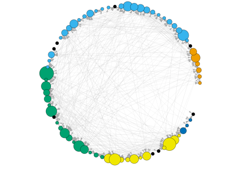
The lawyer network features several stylized facts of a typical real-life network. First, it exhibits degree heterogeneity, the different tendency that the nodes in a network have in participating in network activities as can be seen from Figure 1. Second, the overall network is sparse, in that the observed number of ties does not scale proportionally to the total number of possible links. In Figure 1, the average in- (and out-) degree is 8.1, whereas the maximum possible value is 70. Third, the contextual information in terms of the covariates has a role to play in determining how nodes are connected, as can be seen from the data analysis later. Here the covariates will be denoted as for an edge linking node to . In case where we only have nodal covariates denoted as for the th node, a common approach is to define as a function of and that measures their (dis)similarities.
This paper proposes a new annotated graph model that can effectively deal with the above features in directed networks. This model postulates that links are independently made with the linking probability between node and as
| (1) |
where , , and are parameters. For identifiability, we assume , because otherwise this model becomes trivially the model in Yan et al. (2019) by absorbing into and . Clearly, to fit a model with these many parameters, we will require the number of edges of a network to be relatively large which renders (1) less useful or not even applicable for the kind of networks encountered in practice. To reduce the dimensionality of the model, we assume that both and are sparse. While it may seem appealing to impose instead of , restricting the degree heterogeneity parameters only in absolute value would result in an unidentifiable parameter.
In (1), can be seen as a global density parameter that is allowed to diverge to aiming to model sparse networks. The two node-specific parameters and are used to explicitly capture out- and in-degree heterogeneity respectively. The sparsity assumption on and introduces a notion of differential degree heterogeneity, in the sense that we only include them for nodes that are important. The effect of covariates is captured by . When a covariate encodes the similarity of a node attribute, a positive implies homophily, the tendency of nodes similar in attributes to connect, which is a widely observed phenomenon in real-life networks.
Statistical analysis of random networks has attracted enormous research attention in recent years thanks to a deluge of network data (Kolaczyk, 2009; Fienberg, 2012; Kolaczyk, 2017). Among others, there are several major classes of statistical models that have been successfully applied to model degree heterogeneity, including the stochastic block model aiming to identify groups of nodes as communities (Holland et al., 1983; Bickel and Chen, 2009; Karrer and Newman, 2011; Rohe et al., 2011; Zhao et al., 2012; Lei and Rinaldo, 2015; Gao et al., 2017; Amini and Levina, 2018; Abbe, 2018; Zhang et al., 2021), the -model assigning individual parameters to different nodes (Chatterjee et al., 2011; Yan and Xu, 2013; Yan et al., 2016; Chen et al., 2020), and the exponential random graph models using network motifs as sufficient statistics (Holland and Leinhardt, 1981; Frank and Strauss, 1986; Robins et al., 2007).
The increasing prevalence of covariates in network data calls for models that can effectively account for their effects. For the stochastic block model, we point to Binkiewicz et al. (2017); Zhang et al. (2016); Huang and Feng (2018); Yan and Sarkar (2020). For the -model, see Graham (2017); Yan et al. (2019), and Stein and Leng (2022). Additional references include Ma et al. (2020) where a latent space model approach is investigated and Zhang et al. (2021) that proposes a model-free approach to study the dependence of links on covariates.
Yan et al. (2019) proposed a model similar to (1) with the critical difference that and are dense. As a result, their model only handles relatively dense networks, and the inference on , the covariate parameter, warrants a bias correction step. Remarkable, the inference for this parameter in our model does not require debiasing, even when the network has vanishing link probabilities and hence are sparse. The techniques involved in deriving this result extends substantially many similar ones developed, for example in -estimation (van der Vaart, 1998) and LASSO theory (Ravikumar et al., 2010; van de Geer and Bühlmann, 2011; van de Geer et al., 2014), where the probabilities in similar models are typically assumed to be bounded away from zero.
Another model similar to (1) has been developed for undirected networks by Stein and Leng (2022). The model in this paper is more complex due to the presence of two sets of heterogeneity parameters and thus more delicate analysis is needed (Yan et al., 2016, 2019). More importantly, this paper focuses more on variable selection while Stein and Leng (2022) focused exclusively on estimation consistency. In particular, we place special focus on the study of the interplay of the rates of convergence for the network sparsity, the parameter sparsity and the penalty we use. Each of our main results requires these three quantities to be balanced in a suitable manner, made explicit in our balancing assumptions (Assumptions B1, B2, B3). These assumptions highlight the effect of different sparsity regimes much more clearly than Stein and Leng (2022).
It has been claimed by Barabási (2016) that the degrees of real world networks often follow a power-law distribution. We show in the Appendix D that the degree sequence of the sparse -model in Chen et al. (2020) (as a representative of the family of models introduced in Chen et al. (2020); Stein and Leng (2022) and this paper), follows a power-law distribution under the right assumptions.
1.1 Notation
Denote and . Denote as the non-negative real line. For a vector , we use to denote its support and the -by- diagonal matrix with on the diagonal. Let denote the vector -, - and -norm respectively and define denotes the -“norm”. That is, . For a vector , we number its elements as .
For brevity, we write and . Thus, with its true value denoted as . We write and denote its cardinality by . We write with cardinality to refer to all active indices including those of and . Thus, and can be understood as the parameter sparsity of our model. Let and . When we want to make the dependence of the link probabilities given on different values of explicit, we write . Finally, we use for some generic, strictly positive constant that may change between displays.
For the convenience of the reader, we provide a (non-exhaustive) table of the most important quantities encountered in this paper in Table 1.
| Notation | Description |
|---|---|
| Degree heterogeneity parameters for incomingness and outgoingness | |
| Global sparsity parameter, may diverge to | |
| Covariate parameter, captures homophily, if covariates measure similarity | |
| Shorthand for | |
| The true parameter values | |
| Shorthand for | |
| Shorthand for | |
| The support of with cardinality | |
| , with cardinality | |
| The penalty used in (4) | |
| , the rescaled parameter values | |
| , the rescaled penalty value | |
| out- and in-degree of node respectively | |
| , the excess risk at | |
| Minimum and maximum eigenvalue of respectively | |
| Constant independent of such that and . |
2 Estimation
A directed network on nodes is represented as a directed graph , consisting of a node set with cardinality and an edge set . Without loss of generality, we assume and that is simple, having no self-loops nor multiple edges between any pair of nodes. Such a graph is represented as a binary adjacency matrix , where , if and otherwise. By assumption for all .
Given and the covariates , the negative log-likelihood of the model (1) is
where is the out-degree of vertex and its in-degree. Write and as the corresponding degree sequences. Denote and for which we have . As is common in the literature, we call a network sparse if for some , where is the expectation with regard to the data generating process. A network is dense if .
Since and are sparse, an estimate of can be obtained via the following penalized likelihood
| (2) |
where is a tuning parameter and is the parameter space. For simplicity, we have used the same amount of penalty on and because . The objective function in (2) is similar to the penalized logistic regression with an penalty and thus can be easily solved. In this paper, we use the solver in the R package glmnet (Friedman et al., 2010). The similarity of our estimator to the LASSO estimator makes our estimation approach extremely scalable.
Since our focus is on sparse networks, we assume the existence of a non-random sequence , allowing as , such that for all ,
where is referred to as the network sparsity parameter. The above constraint is equivalent to
where for and since . This inequality can also be expressed in terms of the design matrix associated with the corresponding logistic regression problem, defined in (5) below, and is equivalent to This motivates the following tweak to the estimation procedure in (2): Given a sufficiently large constant , we define the local parameter space
| (3) |
which is convex, and propose to estimate the parameters as
| (4) |
which is more amenable for theoretical analysis.
We now give an explicit form of the associated design matrix . Since we have the presence/ absence of directed edges and parameters, has dimension . Define the out-matrix with rows , such that for each component , if and zero otherwise. Likewise, define the in-matrix with rows , such that for each component , if and zero otherwise. Let be the matrix of the covariate vectors written below each other. Then, the design matrix consists of four blocks, written next to each other:
| (5) |
where is a vector of all ones. We use the shorthand
The design matrix reveals an important property of our model (1). While the columns of the the global parameters and have non-zero entries in all rows of , the local parameters and only have non-zero entries in their respective columns. Thus, the effective sample size for and is only , whereas it is , that is, of order larger, for the global parameters and . This will also be reflected in the different rates of convergence we obtain in Theorem 5 below.
A key quantity in the theory of high-dimensional statistics is the population Gram matrix , closely linked to the Hessian of and the precision matrix. Loosely speaking, it is given by
Were we to naively ignore the differing sample sizes between local and global parameters and choose , our proofs would fail, due to the top-left corner of rapidly converging to the zero-matrix, making singular in the limit. In particular, the compatibility condition (cf. Section 3.2), crucial for proofs for LASSO-type problems, would not hold. We need to account for this fact and therefore propose to use a sample-size adjusted Gram matrix. To that end, we introduce the matrix
where is the identity matrix and define the sample size adjusted Gram matrix as
| (6) |
It will be convenient to cast problem (4) in terms of rescaled parameters which adjust for the discrepancy in effective sample sizes. This new formulation is equivalent to the one in (4), but gives us a unified framework for treating convergence properties of our estimators. We will rely heavily on that rescaled version in our proofs. For now, we simply remark that for any parameter , we introduce the notation
| (7) |
and refer the reader to Section A.2 in the appendix for a derivation and interpretation of this formulation. Our original estimation problem (4) can then equivalently be rewritten in terms of these rescaled parameters, giving rise to a sample-size adjusted estimator
that solves a problem similar to (4) with penalty parameter (see (13) in Section A.2). We denote the negative log-likelihood with respect to a rescaled parameter by . Then, given a solution for a given penalty parameter to this modified problem (13), we can obtain a solution to our original problem (4) with penalty parameter , by setting
| (8) |
3 Theory
We outline the main assumptions first.
Assumption 1
The ’s are independent with and uniformly bounded. We also assume that lies in some compact, convex set with a fixed . Further assume that there are constants such that the minimum eigenvalue and the maximum eigenvalue of fulfil . Without loss of generality we assume .
As a result of Assumption 1, there exist constants such that for all and for all .
Assumption 2
We assume that or equivalently . Therefore, without loss of generality we assume and consequently .
Assumption 1 is standard. Note that ’s are not necessarily i.i.d., possibly having correlated entries and that can be asymmetric in that . We have chosen to focus on the random-design assumption which is somewhat more interesting than a fixed-design one. We have assumed a fixed and leave the study of diverging to future study. Assumption 2 ensures no model misspecification.
Assumption B1
.
For all of our theorems, striking the right balance between parameter sparsity , network sparsity and penalty parameter is crucial. The restrictiveness of these balancing assumptions will depend on the complexity of the results being proven and we number them separately from the general assumptions as “Assumption B”, , to make their special standing explicit in our notation. Our main result on model selection consistency, Theorem 1, is the most refined of our theorems and hence Assumption B1 is the strongest such balancing assumption. In particular, the weaker balancing assumptions required to establish parameter estimation consistency, Theorem 5 (Assumption B2), and asymptotic normality of the homophily parameter estimator , Theorem 6 (Assumption B3), follow from Assumptions B1 above and 3 below. Thus, our estimator in (4) can simultaneously recover the correct support, consistently estimate the parameter values and produce an asymptotically normal estimate of .
3.1 Model selection consistency
In this section we study under which conditions our estimator (4) identifies the correct subset of active variables . Our main result, Theorem 1, is that under the appropriate conditions, our estimator will correctly exclude all the truly inactive parameters and correctly include all those truly active parameters whose value exceeds a certain threshold. The latter minimal signal condition is typical for model selection (Ravikumar et al., 2010; Chen et al., 2020, e.g.).
Recall that we use to refer to the active set of indices associated with , whereas . In the following derivations it will be crucial to distinguish the two correctly. We use to denote the complement of in , that is . Let refer to the complement of in only: . While this may seem like a potential notational pitfall, this allows for much cleaner notation in our proofs.
We first state the main theorem of this section before giving more details on its derivation. Recall that is the penalty parameter in the rescaled version of our problem (4). Also notice that , that is the estimators (4) and (8) will always select the same active set of parameters.
Assumption 3
.
Assumption 3 suggests we pick our penalty of order . Thus, informally speaking, Assumption 3 requires that the rescaled penalty parameter must be at least of order , which is the typical rate for the penalty we would expect from classical LASSO literature (van de Geer and Bühlmann, 2011).
Theorem 1
Under Assumptions 1, 2, B1 and 3, and for sufficiently large, with probability approaching one, the penalized likelihood estimator from (4):
-
1.
excludes all the truly inactive parameters: and,
-
2.
with penalty of order , it includes all those truly active parameters whose value is larger than :
where the form of and the exact probability are given in the proof.
We have the following remarks.
Remark 2
- 1.
-
2.
If we choose and is of lower order, such as growing logarithmically or constant, then, up to log-terms, Assumption B1 implies that we must have for the permissible network sparsity, .
Our tool of choice for proving Theorem 1 is a primal-dual witness construction, similar to the one in Ravikumar et al. (2010). The idea is to construct a tuple , such that solves the rescaled version of (4), while also identifying the correct support and is a solution to the Karush-Kuhn-Tucker conditions (9) as outlined below. In the construction of , we make use of knowledge of the true active set , which makes it infeasible to use in practice. However, by Lemma 3 below, if the construction succeeds – we make precise what we mean by that below – any solution to (4) must have the same support as . In summary, if the construction succeeds, our estimator must identify the correct support , too. The bulk of the work in proving Theorem 1 is to show that the construction of will be successful with high probability for large .
It is important to point out that due to the mixture of deterministic and random columns in and the differing sample sizes between and , the standard assumptions in Ravikumar et al. (2010) imposed on the Hessian of cannot simply be imposed in our model. Rather, a careful argument is needed to prove that analogous properties hold for sufficiently large with high probability. See Section C.1 in the appendix for details.
Our starting point for proving Theorem 1 are the Karush-Kuhn-Tucker conditions (Bertsekas, 1995, Chapter 5): Equation (4) and its rescaled version (13) are a convex optimization problems. Hence, by subdifferential calculus, a vector is a minimizer of (13) if and only if zero is contained in the subdifferential of at . That is, if and only if there is a vector such that
| (9) |
and
| (10a) | ||||
| (10b) | ||||
| (10c) | ||||
We call such a pair primal-dual optimal for the rescaled problem (13). Note that in the first components of we are taking the derivative with respect to instead of . This means we need to pay attention to additional -factors. For such a pair to identify the correct support , it is sufficient for
| (11a) | |||
| (11b) | |||
to hold. Where (11a) ensures that all truly active indices are included and (11b) ensures that all truly inactive indices are excluded (due to (10a)). We call (11b) the strict feasibility condition as in Ravikumar et al. (2010).
We will proceed to construct a pair that satisfies condition (9), (10a) - (10c) and (11a) - (11b) with high probability and for sufficiently large . We say the construction succeeds, if fulfils (9) - (11b), which in particular implies that identifies the correct support and also is a solution to (13).
By the following lemma, if the construction succeeds, any solution to (13) in the appendix must have the same support as . Thus, if the construction succeeds, our estimator must identify the correct support , too.
Lemma 3
We now give a detailed description of the primal-dual witness construction.
Primal-dual witness construction.
-
1.
Solve the restricted penalized likelihood problem
(12) where the argmin is taken over all with support , i.e. or equivalently . Thus, by construction, correctly excludes all inactive indices.
- 2.
- 3.
The challenge will be proving that (11a) and (11b) also hold, which together ensure that (10b) holds, too.
3.2 Consistency
In this section we will show that under assumptions similar to those of Theorem 1, our estimator will also be consistent in terms of excess risk (cf. Greenshtein and Ritov (2004), Koltchinskii (2011)) and -error. To that end, define the excess risk for a parameter as
By construction, where the second equality follows from Assumption 2.
A compatibility condition. A crucial identifiability assumption in LASSO theory is the so called compatibility condition (van de Geer and Bühlmann, 2011; van de Geer et al., 2014). It relates the quantities and
in a suitable sense made precise below and is crucial for deriving consistency results. In our model, similar to the sparse -model in Stein and Leng (2022), the classical compatibility condition as for example defined for generalized linear models in van de Geer et al. (2014) does not hold. The reason for this is that and have different effective sample sizes. Therefore, it is crucial that we use the sample size adjusted Gram matrix (6). Using similar techniques as in Stein and Leng (2022), we can now show that the sample size adjusted Gram matrix fulfils the compatibility condition.
Proposition 4 (Compatibility condition)
Parameter estimation consistency is the most lenient of our theorems in terms of restrictions that we have to impose on the parameter sparsity and the network sparsity . We may replace the stricter assumption B1 by the following.
Assumption B2
.
Theorem 5 below suggests a choice of . Under these conditions, Assumption B2 becomes . That is, up to an additional factor , which is the price we have to pay for allowing our link probabilities to go to zero, the permissible sparsity for is the permissible sparsity in classical LASSO theory for an effective sample size of order . This makes sense, considering the discussion of the differing effective sample sizes in Section 3. Also, this choice of together with Assumption B2 implies , as is required by Proposition 4 and which thus is not a restriction.
Theorem 5
Theorem 5 implies a lower bound on of order , suggesting that we may choose of the same order. Thus, up to the additional factor , we obtain the classical LASSO rates of convergence for a parameter of effective sample size for and and those for a parameter of effective sample size for and . If is a lower order term, such as growing logarithmically or constant, then up to log-factors Assumption B2 requires that tend to zero at rate at most as fast as , which is faster and thus allows for sparser networks than what we obtained for model selection consistency in Theorem 1. Under Assumption B2, we can see that the above average rate of convergence for estimating is slower than the rate for estimating . The rate of convergence for consistency of the estimator is of the same order as the rate obtained for the analogous estimator for undirected networks in Stein and Leng (2022). We refer to Stein and Leng (2022), Section 2.2, for a comparison between -penalized estimation procedures as discussed here and -penalized estimators as advocated by Chen et al. (2020).
3.3 Inference
Finally, we derive the limiting distribution of our estimator of the covariates weights, . We will see that the same arguments used for deriving the limiting distribution for also work for and as a by-product of our proofs we also obtain an analogous limiting result for .
Our strategy will be inverting the Karush-Kuhn-Tucker conditions, similar to van de Geer et al. (2014). See Section B.2 in the appendix for details. Denote by , the Hessian of with respect to only, evaluated at .
Let be the part of the design matrix , defined in (5), corresponding to with rows . Also, let . It is then easy to see
Let and consider the corresponding population version:
To be consistent with commonly used notation, call and and
For the proof of asymptotic normality, we need to invert and and show that these inverses are close to each other in an appropriate sense. It is commonly assumed in LASSO theory (cf. van de Geer et al. (2014)) that the minimum eigenvalues of these matrices stay bounded away from zero. In our case, however, such an assumption is invalid. Since we allow for the lower bound on the link probabilities to go to zero, any lower bound on the entries in will go to zero with and as a consequence our lower bound on the minimum eigenvalue of will tend to zero as goes to infinity as well. The best we can achieve is a strict positive definiteness of for finite , but not uniformly in . Since these lower bounds tend to zero with increasing , a careful argument is needed and we need to impose a slightly stricter balancing assumption than Assumption B2.
Assumption B3
.
Theorem 6
Contrary to what is commonly seen in the penalized likelihood literature (Zhang and Zhang, 2014; van de Geer et al., 2014), no debiasing of and is needed. The reason for this is that columns of pertaining to those parameters which are indeed biased, that is to , and those pertaining to become asymptotically orthogonal, meaning that the bias in vanishes fast enough for the derivation of Theorem 6 to be possible. For a lower order , Assumption B3 essentially allows for the same level of network sparsity as Assumption B1, up to lower order factors.
4 Simulation
In this section we demonstrate the effectiveness of our estimator (4) in performing simultaneous parameter estimation and model selection consistently. To this end, we test its performance on networks of varying sizes. Specifically, we let vary between and in steps of and choose the sparsity level to be close to . We let and chose in each case. We selected a heterogeneous configuration for the assignment of non-zero and values. That is, we included dedicated ‘spreader’ nodes, with large and zero value as well as ‘attractor’ nodes with large and zero as well as some nodes with both active and . In detail, we let
where the number of entries with value was chosen to match the aforementioned sparsity level (zero for the first three values of ) and the number of leading zeros in was chosen such that there were exactly two nodes with both active and . We let the networks get progressively sparser and set . In all cases we used , sampled the covariate values from a centred distribution, and set . Our estimator requires us to choose a tuning parameter and we explored the use of the Bayesian Information Criterion (BIC) as well as a heuristic based on our developed theory for model selection. While the former criterion is purely data-driven, the use of the latter is to ensure that our theoretical results are about right in terms of the rates. Specifically, our BIC is defined as
where is the solution with as the tuning parameter, and is the cardinality of its support. On the other hand, our heuristic is motivated by the theory developed in the previous sections. We construct as in Theorem 5 based on confidence level , choosing to drop the leading factor eight prescribed by Theorem 5. It is known that in high-dimensional settings the penalty values prescribed by mathematical theory in practice tend to over-penalize the parameter values (Yu et al., 2019). Decreasing the penalty by removing that factor is thus in line with these empirical findings.
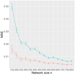
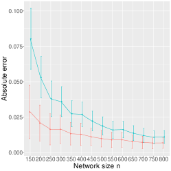
We drew realizations for each value of and recorded the mean absolute error for estimation of , the absolute error for estimation of and the -error for estimation of . We also constructed confidence intervals as prescribed by Theorem 6 and recorded the empirical coverage at the nominal level. Finally, we studied how well BIC and our heuristic did in terms of identifying the correct model.
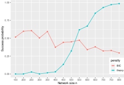
Consistency. We display the various error statistics for estimation of and in Figures 2(a), 2(b) and 2(c) respectively. We see that the error decreases with increasing network size for both model selection procedures. We see that especially for small , BIC outperforms the heuristic for and , while they both give essentially the same results for estimation of . The better performance of BIC is less prominent as increases. BIC selects the penalty in a purely data driven manner, which allows it to adapt to differing degrees of sparsity in the network, while for the heuristic the penalty value only depends on and . This additional flexibility is what allows BIC to achieve lower error values.
Asymptotic normality. We construct confidence intervals at the nominal 95% level for our estimators of and as prescribed by Theorem 6. Table 2 shows the results for across three values of . The results for other and are similar and are omitted to save space. The coverage is very close to the -level across all network sizes, independent of which model selection criterion we use. This is to be expected, considering that there was hardly any difference for the estimation of between our two model selection criteria. This empirically illustrates the validity of the asymptotic results derived in Theorem 6. As expected, the median length of the confidence interval decreases with increasing network size.
| Coverage | CI | Coverage | CI | ||
|---|---|---|---|---|---|
| Heuristic | BIC | ||||
| 200 | 0.952 | 0.265 | 0.962 | 0.266 | |
| 400 | 0.950 | 0.141 | 0.964 | 0.141 | |
| 800 | 0.946 | 0.075 | 0.952 | 0.075 | |
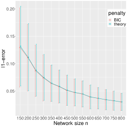
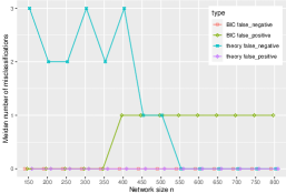
Model selection. Finally we compare model selection performance between BIC and our heuristic. Figure 3(a) shows the empirical probability of selecting the correct model versus the various network sizes. We can see very clearly that asymptotically, as grows, our heuristic outperforms BIC, achieving correct model selection almost all the time. Nonetheless, it is worth pointing out that even though BIC may not select the exact correct model, the number of misclassifications it does on average is not very large, as shown in Figure 3(b). Figure 3(b) also shows that the heuristic, by virtue of selecting a larger penalty than BIC, will on average incur more false negatives for small . On the other hand, as grows, BIC will incur false positives, resulting in the decreasing probability of selecting the correct subset.
4.1 The lawyer data
We return to our motivating example by comparing our estimates of the regression coefficients with those in Yan et al. (2019). For the seven covariates in this dataset, we followed Yan et al. (2019) in using the absolute differences of the continuous variables and the indicators whether the categorical variables are equal as our covariates. The edge density in this network is .
To apply the model in Yan et al. (2019), one needs to remove the eight nodes in black in Figure 1 that have zero in-degree or out-degree. Otherwise the maximum likelihood estimates would be for if node has no outgoing connections or for if the node has no incoming links. Another interesting aspect of the model in Yan et al. (2019) lies in the inference for the fixed-dimensional parameter . Because the rate of convergence of its estimate is slowed down by those of the growing-dimensional heterogeneity parameters and , the estimator of requires a bias correction to be asymptotically normal. In contrast, by making a sparsity assumption on and in our model, we estimate the parameters via penalized likelihood and the inference of is straightforward as seen in Theorem 6.
When the Bayesian information criterion is used to choose the tuning parameter in the penalized likelihood estimation, our model gives 7 nonzero ’s and nonzero ’s. Four pairs of these nonzeros come from the same nodes. In Table 3 we present the estimated and their standard errors when our model and the model in Yan et al. (2019) are fitted. We remark that since Yan et al. (2019) removed eight nodes, akin to biased sampling, their estimates can be biased. In terms of the parameter estimates themselves, although generally similar, we can see a few differences. First we can see that the standard errors of our estimates are smaller than those in Yan et al. (2019), reflecting that our estimates are based on a larger sample size (a network with 71 nodes compared to one with 63 nodes in the latter paper) with fewer parameters (22 versus 132). Second, the effect of age difference is not significant in our model while it is in the model in Yan et al. (2019). To explore the age effect graphically, we colour-coded the lawyers by their age group in Figure 1. We can see that plenty of connections are made between age groups and ”across the circle”, i.e. between lawyers with a large difference in age, suggesting that age may not have played an important role. Indeed, a third () of all friendships are formed between lawyers with an age difference of ten or more years. Third, we estimate the effect of attending the same law school as positive, implying that the lawyers tend to befriend those who graduated from the same school, while Yan et al.’s model states the opposite. The former conforms better to our intuition about social networks.
| This Paper | Yan et al. (2019) | |||
|---|---|---|---|---|
| Covariate | Estimate | SE | Estimate | SE |
| Same status | ||||
| Same gender | ||||
| Same office | ||||
| Same practice | ||||
| Same law school | ||||
| Difference in years with firm | ||||
| Difference in age | ||||
4.2 Link prediction for the lawyer data
In this section we give a brief illustration of how our model can be used for link prediction. We remark that in general it is not possible to conduct vanilla train-test splits or cross-validation on network data, since randomly removing nodes or edges can destroy part of the network structure (Li et al., 2020). While some prior work on network cross-validation exists, notably the aforementioned paper, developing a rigorous cross-validation scheme for our model is beyond the scope of the current paper. Therefore, we present the results in this section as a guideline that the present model shows promising performance for link prediction, even when using vanilla cross-validation. We leave the rigorous mathematical treatment of this interesting problem for a future paper.
In the following, we mimic traditional K-fold cross-validation with K=10 for this dataset as follows. We randomly split the entries of the adjacency matrix of the lawyer data into 10 folds (ignoring the diagonal). This corresponds to randomly selecting node pairs, as advocated in Li et al. (2020). For each fold, we fit our model on the other 90% of of the entries of and use the fitted model to predict the values for the 10% holdout fold. We run 10 repetitions of this modified 10-fold cross-validation and present the results in Figure 4. As we can see, even when using this vanilla approach, we achieve a decent performance in the high 80% range usually, which suggests that with some further adjustments it might be possible to derive strong theoretical guarantees for link prediction for the present model. The key ingredient for why we believe this could be a fruitful research avenue is that link formation happens independently, conditional on the values of the covariates .
4.3 Sina Weibo data
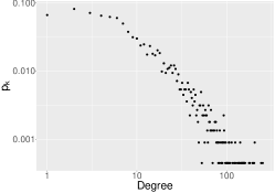
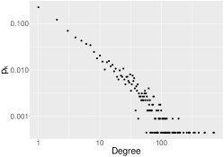
In our second case study we explore how well our estimation procedure scales to large networks. Towards this, we study the Sina Weibo data collected by Cai et al. (2018), which was also analysed in Yan et al. (2019). Sina Weibo is a Chinese social media platform similar to Twitter. In the original data set there are 4077 nodes representing MBA students and directed links represent who follows whom. Following Yan et al. (2019), we focus on the largest strongly connected component consisting of 2242 nodes, leaving us with a very sparse network in which only of all possible edges are observed. The resulting in- and out-degree sequences have heavy tails, meaning this network also exhibits a high degree of degree heterogeneity, as illustrated in Figure 5. The in-degrees range from 1 to 253, with the first quartile, median and third quartile equal to 4, 9 and 22 respectively. For the out-degrees we observe values between 1 and 715, with first quartile, median and third quartile equal to 2, 5 and 19 respectively.
For each node we observe the number of posts they have written, their tenure (measured in months since they joined the platform) and the number of characters in personal labels which were created by the users to describe their lifestyle. We used the absolute difference between these variables as covariates and standardized their values before fitting our model to the data using BIC. In Table 4 we compare the estimates for and their standard errors when our model is fitted with the results obtained by Yan et al. (2019). While both papers estimate all covariates as significant with a negative sign, it is noteworthy that Yan et al. (2019) initially obtained positive covariate estimates for the difference in the number of posts and labels. Only after running their bias-correction procedure did they obtain the estimates presented here, which illustrates that indeed this ad-hoc procedure is necessary for their model to work properly. On the other hand, we obtain the the negative signs right off-the bat, while also giving us smaller standard errors.
| This Paper | Yan et al. (2019) | |||
|---|---|---|---|---|
| Covariate | Estimate | SE | Estimate | SE |
| Difference in posts | ||||
| Difference in tenure | ||||
| Difference in number of labels | ||||
5 Discussion
We have assumed that links are formed independently between node pairs. This is a limitation because empirically reciprocity, a measure of the likelihood of vertices in a directed network to be mutually linked, may be present. In the motivating lawyers data for example, lawyer will be more likely to call lawyer a friend if the converse is true. To address this layer of sophistication, the next natural step is to add a reciprocity parameter to the model. In this paper, we have focused on the inference of the covariate parameter. In some applications inference on and may be of interest. Since their estimates are biased due to the shrinkage incurred by our penalty, this will require debiasing, possibly coupled with suitable balancing assumptions. We leave the exploration of these two interesting research questions for future work.
Acknowledgments
We thank the Action Editor and two reviewers for their very helpful comments that have led to a much improved paper.
Appendix A Appendix A
We introduce the following additional notation.
For any we use the notation and . For any subset , we denote by the vector with components not belonging to set to zero. For a matrix and a subset , denote by the submatrix of obtained by only taking the rows and columns belonging to . Denote by the submatrix obtained by keeping all the rows and taking only those columns belonging to and by the submatrix obtained by taking only those rows belonging to and keeping all the columns. For any square matrix , we denote by its maximum eigenvalue and by its minimum eigenvalue.
A.1 A compatibility condition
In this section we first prove a sample compatibility condition before providing a proof for the population compatibility condition in Proposition 4. That is, we first want to find a suitable relation between the quantities and where is the sample version of the sample size adjusted Gram matrix .
We make this mathematically precise now: For a general matrix we say the compatibility condition holds, if has the following property: There is a constant independent of such that for every with it holds that
Notice that the compatibility condition is clearly equivalent to the condition that
stays bounded away from zero.
We first show that the compatibility condition holds for the matrix
where is the identity matrix.
Recall that by assumption 1, the minimum eigenvalue of stays uniformly bounded away from zero. That is, there is a finite constant independent of , such that for all . Then, clearly, for any ,
Thus, is strictly positive definite. Furthermore, by Cauchy-Schwarz’ inequality, for any with ,
Thus,
We conclude that the compatibility condition holds for . Now, we need to show that with high probability , which would imply that the compatibility condition holds with high probability for . To that end, we have the following auxiliary lemma found in Kock and Tang (2019). For completeness, we give the short proof of it. The notation is adapted to our setting.
Lemma 7 (Lemma 6 in Kock and Tang (2019))
Let and be two positive semi-definite matrices and . For any set with cardinality , one has
Proof Denote by and . Let , with . Then,
Hence, and thus
Minimizing the left-hand side over all with proves the claim.
This shows that to control , we need to control the maximum element-wise distance between and : .
Introduce the set
On the set , by Lemma 7, we have and thus the compatibility condition holds for on .
Lemma 8
If , for large enough, with and , where is the universal constant such that for all , we have
Proof To make referencing of sections of easier, we number its blocks as follows
For block , i.e. , notice that and is a matrix with zero on the diagonal and ones everywhere else. Therefore, we have either or
for large enough, since . Blocks and are a dimensional column and row vector respectively in which each entry is equal to . Thus, for corresponding to these blocks,
for large enough, since . For corresponding to blocks and , we have
for large enough. Block is a single real number and equal for and .
The only cases left to consider are those entries corresponding to blocks ⑥, ⑧ and ⑨. For the blocks ⑥ and ⑧, that is for and , is the scaled sum of all the entries of some column of the matrix for an appropriate . That is, there is a such that
Note, that thus by model assumption . We know that for each . Hence, by Hoeffding’s inequality, for all ,
For block ⑨, that is for , a typical element has the form
for appropriate . In other words, is the inner product of two columns of , minus their expectation, scaled by . Since for all , we have that for all : . Thus, by Hoeffding’s inequality, for all ,
Thus, with , we have for any entry in blocks ⑥, ⑧, ⑨, that for any ,
Choosing , by the exposition above we know that all entries in blocks ① - ⑤ and ⑦ are bounded by for . Also, because block ⑥ is the transpose of block ⑧, it is sufficient to control one of them. By symmetry of block ⑨ it suffices to control the upper triangular half, including the diagonal, of block ⑨. Thus, we only need to control the entries for in the following index set
Keep in mind that block ⑧ has elements, while the upper triangular part of block ⑨ plus its diagonal has elements. Thus, for ,
This proves the claim.
We summarize these results in the following proposition
Proposition 9
Under Assumption 1, for and large enough, with , where is the universal constant such that for all : With probability at least
it holds that for every with ,
Proof
This follows from Lemma 8.
Proof [Proof of Proposition 4] To prove that the compatibility condition holds for the population sample-size adjusted Gram matrix we may follow the same steps as in the proof of Proposition 9: Number the blocks of as ① - ⑨ as we did for . and are equal on blocks ③, ⑤, ⑥, ⑦, ⑧ and ⑨. For blocks ①, ② and ④ we use the exact same arguments as in the proof of Proposition 9 to find that for sufficiently large, almost surely,
The claim follows from Lemma 7.
A.2 A rescaled estimation problem
We now formally introduce the notion of sample-size adjusted parameters . Precisely, define the sample size adjusted design matrix as
where
is blowing up the entries in belonging to . Recall that for any parameter , we use
to refer to its sample-size adjusted version. In particular we use the notation , to denote the re-parametrized true parameter value. The blow-up factor was chosen precisely such that we can now reformulate our problem as a problem in which each parameter effectively has sample size in the sense that
Our original penalized likelihood problem can be rewritten as
| (13) | ||||
where and the argmin is taken over . Note that by the same arguments as before, is convex. Then, given a solution for a given penalty parameter to this modified problem (13), we can obtain a solution to our original problem (4) with penalty parameter , by setting
Note that for any , , and hence the bound is the same in the definitions of and . Note also that if and only if . For any , denote the negative log-likelihood function corresponding to the rescaled problem (13) as . Then, clearly and . Thus, satisfies that We define the excess risk for a sample-size adjusted parameter as
By construction, .
A.3 A basic Inequality
A key result in the consistency proofs in classical LASSO settings is the so called basic inequality (cf. van de Geer and Bühlmann (2011), Chapter 6). Let denote the empirical measure with respect to our observations , that is, for any suitable function ,
In particular, if we let for each , , then Similarly, we define the theoretical risk as . In particular,
where we suppress the dependence of the theoretical risk on in our notation. We may write the excess risk as
We define the empirical process as
Lemma 10 (Basic Inequality)
For any it holds
Proof By plugging in the definitions and rearranging, we see that the above equation is equivalent to
which is true by definition of .
Notice that since the basic inequality in Lemma 10 only relies on the argmin property of the estimator , an analogous result follows line by line for the rescaled parameter . Writing
for the rescaled empirical process, we have the following.
Lemma 11
For any it holds
Remark 12
For any and , let . Since is convex, and since and are convex functions, we can replace by in the basic inequality and still obtain the same result. Plugging in the definitions, we see that the basic inequality is equivalent to the following:
and by convexity
where the last inequality follows by definition of . In particular, for any , choosing
gives . The completely analogous result holds for .
A.4 Two norms and one function space
To give us a more compact way of writing, for any we introduce functions and denote the function space of all such by . We endow with two norms as follows:
Denote the law of the rows of on , i.e. the probability measure induced by , by . That is, for a measurable set ,
where if and zero otherwise, is the Dirac-measure. We are interested in the and norm on with respect to the measure on . Denote the -norm of simply by and let be the expectation with respect to :
and define the -norm as usual as the -a.s. smallest upper bound of :
Notice in particular, that for any : .
We make the analogous definitions for the unscaled design matrix. Let denote the probability measure induced by the rows of . Since , for any with rescaled version , we have
We want to apply the compatibility condition to vectors of the form .
Notice, that we have the following relation between the -norm and the sample size adjusted Gram matrix : For any we have
| (14) |
We have the following corollary which follows immediately from Proposition 4 (see e.g. van de Geer and Bühlmann (2011), section 6.12 for a general treatment).
Corollary 13
Under assumption 1, for and large enough and with , where is the universal constant such that for all , it holds that for every with ,
where .
A.5 Lower quadratic margin for
In this section we will derive a lower quadratic bound on the excess risk if the parameter is close to the truth . This is a necessary property for the proof to come and is referred to as the margin condition in classical LASSO theory (cf. van de Geer and Bühlmann (2011)).
The proof mainly relies on a second order Taylor expansion of the function of introduced in section 3. Given a fixed , we treat as a function in and define new functions
where and by slight abuse of notation we use . Taking derivations, it is easy to see that
All are clearly twice continuously differentiable with derivative
Using a second order Taylor expansion around we get
with an between and . Note that . Then, for any with , we must have that for any intermediate point between and it also holds that . Also note that is symmetric and monotone decreasing for . Thus, for any with ,
| (15) | ||||
In particular, if we pick any and let , we have
Let
| (16) |
Define a subset as . Now, for all :
Thus, we have obtained a lower bound for the excess risk given by the quadratic function where . Recall that the convex conjugate of a strictly convex function on with is defined as the function
and in particular, if for a positive constant , we have . Hence, the convex conjugate of is
Keep in mind that by definition for any
A.6 Consistency on a special set
In this section we will show that the penalized likelihood estimator is consistent. We will first define a set and show that consistency holds on . It will then suffice to show that the probability of tends to one as well. The proof follows in spirit van de Geer and Bühlmann (2011), Theorem 6.4.
We define some objects that we will need for the proof of consistency. We want to use the quadratic margin condition derived in section A.5. Recall that the quadratic margin condition holds for any . Define
Recall the definition of in equation (7) and let for any
where denotes the empirical process. The set over which we are maximizing in the definition of can be expressed in terms of parameters on the original scale as
Set
where is a lower bound on that will be made precise in the proof showing that has large probability. Define
| (17) |
Proof [Proof of Theorem 14] We assume that we are on the set throughout. Set
and . Then,
Since and by the convexity of , , and by the remark after Lemma 11, the basic inequality holds for . Also, recall that :
From now on write . Note, that and thus, by the triangle inequality,
| (18) | ||||
Case i) If , then
| (19) |
Since , we may thus apply the compatibility condition corollary 13 (note that ) to obtain
where we have used that is linear and hence . Observe that
| (20) |
Hence,
Recall that for a convex function and its convex conjugate we have . Thus, we obtain
It follows
and therefore
| (21) |
Finally, this gives
From this, by using the definition of , we obtain
Rearranging gives
Case ii) If , then from (18)
Using once more (20), we get
| (22) |
Thus,
by choice of . Again, plugging in the definition of , we obtain
Hence, in either case we have . That means, we can repeat the above steps with instead of : Writing , following the same reasoning as above we arrive once more at (18):
From this, in case i) we obtain (19) which allows us to use the compatibility assumption to arrive at (21):
resulting in
In case ii) on the other hand, we arrive directly at (22), and hence
Plugging in the definitions of and and using the fact that proves the claim.
A.7 Controlling the special set
We now show that has probability tending to one. Recall some results on concentration inequalities.
Concentration inequalities
We first recall some probability inequalities that we will need. This is based on chapter 14 in van de Geer and Bühlmann (2011). Throughout let be a sequence of independent random variables in some space and be a class of real valued functions on .
Definition 15
A Rademacher sequence is a sequence of i.i.d. random variables with for all .
Theorem 16 (Symmetrization Theorem as in van der Vaart and Wellner (1996), abridged)
Let be a Rademacher sequence independent of . Then
Theorem 17 (Contraction Theorem as in Ledoux and Talagrand (1991))
Let be non-random elements of and let be a class of real-valued functions on . Consider Lipschitz functions with Lipschitz constant , i.e. for all
Let be a Rademacher sequence. Then for any function we have
The last theorem we need is a concentration inequality due to Bousquet (2002). We give a version as presented in van de Geer (2008).
Theorem 18 (Bousequet’s concentration theorem)
Suppose and all satisfy the following conditions for some real valued constants and
and
Define
Then for any
Remark 19
Looking at the original paper of Bousquet (2002), their result looks quite different at first. To see that the above falls into their framework, set the variables in Bousquet (2002) as follows
Now apply Theorem 2.1 in Bousquet (2002), choosing for their the above defined , for their the above defined and setting and in their theorem: The result is exactly Theorem 18 above.
Finally we have a Lemma derived from Hoeffding’s inequality. The proof can be found in van de Geer and Bühlmann (2011), Lemma 14.14 (here we use the special case of their Lemma for ).
Lemma 20
Let be a set of real valued functions on satisfying for all and all
for some positive constants . Then
The expectation of
Recall the definition of
where denotes the re-parametrized empirical process. Recall, that there is a constant such that uniformly .
Lemma 21
For any we have
Proof Let be a Rademacher sequence independent of . We first want to use the symmetrization theorem 16: For the random variables we choose . For any we consider the functions
and the function set . Note, that
Then, the symmetrization theorem gives us
Next, we want to apply the contraction Theorem 17. Denote and let be the conditional expectation given . We need the conditional expectation at this point, because Theorem 17 requires non-random arguments in the functions. This does not hinder us, as later we will simply take iterated expectations, cancelling out the conditional expectation, see below. For the functions in Theorem 17 we choose
Note, that has derivative bounded by one and thus is Lipschitz continuous with constant one by the Mean Value Theorem. Thus, all are also Lipschitz continuous with constant :
For the function class in Theorem 17 we choose and pick . Then, by Theorem 17
Recall that we can express the functions as
where is the projection on the -th coordinate. Consider any with . For the sake of a compact representation we use our shorthand notation where the components are defined in the canonical way and we also simply write for the projection of the the vector to its -th component, i.e. instead of . Then,
Note, that the last expression no longer depends on . To bind the right hand side in the last expression we use Lemma 20: In the language of the Lemma, choose as . We choose for the in the formulation of the Lemma and pick for our functions
Note, that then . We want to employ Lemma 20 which requires us to bound for all and .
For any fixed we have
Note that the first case occurs exactly times for each . Thus, for any ,
If , and hence
Finally, if , and therefore,
In total, this means
Therefore, an application of Lemma 20 results in
Putting everything together, we obtain
This concludes the proof.
We now want to show that does not deviate too far from its expectation. The proof relies on the concentration theorem due to Bousquet, Theorem 18.
Corollary 22
Pick any confidence level . Let
and choose as
Then, we have the inequality
Proof We want to apply Bousquet’s concentration Theorem 18. For the random variables in the formulation of the theorem we choose once more and as functions we consider
Then, we have
To apply Theorem 18, we need to bound the infinity norm of . Recall that we denote the distribution of by and the infinity norm is defined as the -almost sure smallest upper bound on the value of . We have for any , using the Lipschitz continuity of :
| Thus, | ||||
For the last inequality we used that for any with it follows that , which is possibly a very generous upper bound. This does not matter, however, as the term associated with the above bound will be negligible, as we shall see.
The second requirement of Theorem 18 is that the average variance of has to be uniformly bounded. To that end we calculate
Let us look at these terms in term. For the first term, we obtain
For the second term we get
The last term decomposes as
For the first term in that decomposition we have
and for the second term using the same arguments, we get
Meaning that in total
In total, we thus get
| (23) |
Furthermore,
Recall that for any and note that
Then, from the above
| (24) | ||||
Notice that for the second summand on the right-hand side in (23), we have
So that we may use the same steps as in (24) to conclude that
Such that in total,
Applying Bousquet’s concentration Theorem 18 with defined above, we obtain for all
| (25) | ||||
From Lemma 21, we know
Using this, we obtain from (25)
Now, pick to get
which is the claim.
A.8 Putting it all together
Appendix B Proof of Theorem 6
B.1 Inverting population and sample Gram matrices
Note that the function is monotonically increasing in for and monotonically decreasing in for . Thus, by considering the cases and separately and using that , we may employ the following lower bound for all : . Also, recall that by assumption 1, the minimum eigenvalue of stays uniformly bounded away from zero for all . Then, for any and with components , we have
Hence, for finite all eigenvalues of are strictly positive and consequently this matrix is invertible. We now want to show that the same hold with high probability for the sample matrix . Using the tools deployed in the proofs of Lemma 7 and 8 we can now show that with high probability the minimum eigenvalue of is also strictly larger than zero, which means that is invertible with high probability, from which the desired properties of follow. More precisely, recall the definition of for square matrices and dimensions . We want to consider the expression which simplifies to
and compare it to . By assumption 1 and the argument above, we have
for a universal constant independent of . With , by Lemma 7, we have
By looking at the proof of Lemma 7, we see that in this particular case we do not even need the factor on the right hand side above, but this does not matter anyways, so we keep it. By the exact same arguments we have used in the proof of Lemma 8 for the blocks ⑤, ⑥, ⑧ and ⑨, we now get
Thus, for large enough, we have with high probability . Then, by Lemma 7, with high probability and uniformly in ,
Yet, if uniformly in , then for any . But we also know that the minimum eigenvalue of is the largest possible such that this bound holds (it is actually tight with equality for the eigenvectors corresponding to the minimum eigenvalue). Therefore, with high probability, the minimum eigenvalue of stays uniformly bounded away from zero. Thus, for any and any finite :
Thus, . That is, for every finite , is invertible with high probability.
B.2 Goal and approach
Our strategy will be inverting the KKT conditions, similar to van de Geer et al. (2014). Recall our discussion of the KKT conditions in Section 3.1. By the same arguments, we find that has to be contained in the subdifferential of at , where this time we consider the KKT conditions with respect to the original parameters . That is, there exists a such that
where is the gradient of evaluated at and for if and if , and for .
Denoting the gradient of with respect to the unpenalized parameters only, evaluated at , we have
| (26) |
Goal: We want to show that for ,
Approach: Recall the definition of the ”one-sample-version” of , i.e. , for ,
Then, the negative log-likelihood is given by
and
where denotes the Hessian with respect to . Consider as a function in and introduce:
| (27) |
with second derivative: . Note, that is Lipschitz continuous (it has bounded derivative ; Lipschitz continuity then follows by the Mean Value Theorem). Doing a first order Taylor expansion in of in the point evaluated at , we get
| (28) |
for an between and . By Lipschitz continuity of , we also find
| (29) | ||||
where the last inequality follows, because is between and .
Consider the vector : By equation (28), with between and ,
| which by (29) gives | ||||
| Noticing that and thus : | ||||
where the notation is to be understood componentwise. Above, we have equality of two -vectors. We are only interested in the portion relating to , that is, in the last entries. Introduce the -matrix
where 0 are zero-matrices of appropriate dimensions. Multiplying the above with on both sides gives:
| (30) |
Let us consider these terms in turn: Multiplication by means that the first entries of any of the vectors above are zero. Hence we only need to consider the last entries. The left-hand side of (30) is equal to zero by (26). The last entries of the first term on the right-hand side are . For the second term on the right hand side, notice that
is the exact inverse of which is the lower-right block of above matrix. Thus,
Then, for the last entries of
Thus, (30) implies
which is equivalent to
| (31) |
Our goal is now to show that for each component ,
as described in the Goal section. To that end, by equation (31), we now need to solve the following three problems: Writing for the -th row of ,
-
1.
,
-
2.
-
3.
B.3 Bounding inverses
The problems (1) - (3) above suggest that it will be essential to bound the norm and the distance of and in an appropriate manner. Notice that for any invertible matrices we have
Thus, for any sub-multiplicative matrix norm , we get
| (32) |
We are particularly interested in the matrix -norm, defined as
i.e. is the maximal row -norm of . It is well-known, that any such matrix norm induced by a vector norm is sub-multiplicative () and consistent with the inducing vector norm ( for any vector of appropriate dimension). We first want to bound the matrix -norm in terms of the largest eigenvalue.
Lemma 23
For any symmetric, positive semi-definite -matrix with maximal eigenvalue , we have .
Proof
where is the spectral norm of the matrix and we have used that for symmetric matrices, the spectral norm is equal to the modulus of the largest eigenvalue of .
Also, recall that the inverse of a symmetric matrix is itself symmetric:
Hence, and are symmetric and we may apply Lemma 23. Using that , we get
and with high probability
with some absolute constant . Finally, by (32),
It remains to control . We have
Recall that , with the function defined in (27). Also recall that is Lipschitz with constant one, by the Mean Value Theorem and the fact that it has derivative bounded by one. Thus, considering the -th element of above, we get:
Since the dimension of is and thus remains fixed, any row of has norm of order and thus
Taking a look at the -th element in :
Note that the random variables are bounded uniformly in . Thus, by Hoeffding’s inequality, for any ,
This means, . Again, since the dimension is fixed, we get by a simple union bound
In total, we thus get
We can now obtain a rate for .
By assumption B3, we have , which in particular also implies that the above is . Notice in particular, that we have now managed to get for
-
•
,
-
•
.
B.4 Problem 1
We can now take a look at the problems (1) - (3) outlined above. For problem (1), we want to show:
Step 1: Show that
| (33) |
We have
Consider the vector . The -th component of it has the form for and . Notice that for these components are all centred:
as well as , where is a universal constant bounding for all . Thus, by Hoeffding’s inequality, for any ,
and thus,
Since we have , by section B.3, step 1 is now concluded.
Step 2: Show that
Step 3: Show that
for some universal constant . Then, we may conclude from step 1 and step 2 that
To prove step 3, notice that is symmetric and hence has only real eigenvalues. Therefore it is unitarily diagonalizable and for any , we have . We also know that
Under assumption 1 we can now deduce an upper bound on the maximum eigenvalue of : For any ,
where we have used that any entry in is bounded above by one. Since and since this bound is tight (we have equality if is an eigenvector corresponding to ), we can conclude by assumption 1 that for some universal constant .
In particular, since , we get
uniformly for all . Consequently,
Step 3 is thus concluded.
Step 4: Finally, show that
Such that by all the above
For brevity, we write for the true link probabilities . Also keep in mind that denotes the -th row of , while denote -column vectors. We want to apply the Lindeberg-Feller Central Limit Theorem. The random variables we study are the summands in
First, notice that these random variables are centred:
For the Lindeberg-Feller CLT we need to sum up the variances of these random variables. We claim that
Indeed, consider the vector-valued random variable . It has covariance matrix
Thus, by independence across ,
where for the last equality we have used that is the inverse of and thus, . Now, we need to show that the Lindeberg condition holds. That is, we want that for any ,
| (34) |
We have
At the same time, we know from step 3 that for some universal . Then, as long as goes to infinity at a rate slower than , which is enforced by assumption B3, we must have for large enough
uniformly in . Thus, the indicator function and therefore each summand in (34) is equal to zero for large enough. Hence, (34) holds. Then, by the Lindeberg-Feller CLT,
Now, by steps 1-4,
This concludes solving problem 1.
B.5 Problem 2
For problem 2 we must show
Since we have , we do not need to worry about , because and , i.e. . By Theorem 5 we also have a high-probability error bound on . The problem will be bounding the corresponding matrix norms.
Notice that in the display above we have the vector -norm. Also,
Here we used the compatibility of the matrix -norm with the vector -norm. The first term is the vector norm, the second the matrix norm. We know,
where on the left hand side we have the vector norm and in the middle display the matrix norm. Finally, is a -matrix. The -th element looks like , where is the sum of terms of the form , summed over the appropriate indices , all of which are uniformly bounded. Thus,
Thus, the -norm of any row of is bounded by and thus
Recall that by Theorem 5. Then,
Multiplying by , gives
which is under Assumption B3.
B.6 Problem 3
Finally, we must show
Again, since and uniformly in , we do not need to worry about the factor and it remains to show
We have
where for the last inequality we have used that . Now remember from (24) that
where we make use of the fact that . From Theorem 5 we know that under the assumptions of Theorem 6, . Thus,
We see that this is by applying assumption B3 twice. Problem 3 is solved.
Appendix C Proof of Theorem 1
C.1 Proof of Lemmas
To make the representation cleaner, for the remainder of Section C we will simply write for and for . Recall that we use to denote the complement of in , that is . We also use to refer to the complement of in only: .
We begin by providing proofs of the lemmas in section 3.1.
Proof [of Lemma 3] Since and both solve (13), we must have
Denote by the first components of . Then, by (10a) and (10b), . Thus,
| Hence, using that the last components of are zero, | |||
| But by (9), and therefore | |||
By the convexity of , the left-hand side in the above display is negative. Therefore,
Hence, . But since by (11b), this can only hold if . The claim follows.
For the proof of Theorem 1 we need conditions similar to the ones in Ravikumar et al. (2010). The first condition is the so-called dependency condition which demands that the population Hessian of with respect to the variables contained in the active set is invertible. For our specific case, we let
| (35) |
where , be the Hessian of with respect to only.
Lemma 24 (Dependency condition)
For any , the minimum eigenvalue of satisfies
Proof [of Lemma 24] Notice that
where is the identity matrix and is a matrix with zeros on the diagonal and everywhere else. Now consider the submatrix with only those rows and columns belonging to
This matrix is strictly diagonally dominant. Indeed,
where the strict inequalities hold because . Thus, is strictly positive definite. More, by the Gershgorin Circle Theorem, all the eigenvalues of must lie in one of the discs , where and is the disc with radius centred at . In particular,
But now, for any ,
and the claim follows.
Lemma 25 (Incoherence condition)
For any ,
By Lemma 24 the left-hand side of Lemma 25 is well-defined. Furthermore, under Assumption B1, the right-hand side in Lemma 25 tends to zero as tends to infinity.
Proof [of Lemma 25] We make use of the following bound of a the infinity norm of the inverse of a diagonally dominant matrix (see for example Varah (1975))
where is the th diagonal entry of and is the sum of the off-diagonal elements of the th row of . That is, for ,
and analogously for ,
Thus,
and therefore,
| (36) |
Furthermore, notice that any row of has either or non-zero entries, each of the form . Hence,
The claim follows by the submultiplicativity of the matrix infinity norm.
C.2 General strategy
The proof of Theorem 1 hinges on the construction of succeeding with high probability and the challenge in proving this is proving that fulfils conditions (11a) and (11b). Our proof relies on the following derivations. From (9) we obtain
Doing a Taylor expansion along the same lines as (28) and (29), we obtain
where we have used the fact that we are taking derivatives with respect to and used in (29), to obtain instead of above. Combining the last two equations, we obtain
Taking only the first entries of that equation we obtain
| (37) | ||||
where we use to refer to the first components of , use our shorthand notation and let
Notice that we the left-hand side in (37) is equal to
Plugging this into (37) and splitting up by rows, we get
| (38b) | ||||
| (38d) | ||||
where it is important to remember that refers to the complement of in . We solve (38b) for and plug the result into (38d). Finally we rearrange for ,
Now, divide by and take the -norm on both sides. Rearrange corresponding terms.
By appropriately bounding the terms on the right-hand side, we will proceed to show that for sufficiently large , with high probability, , which is clearly equivalent to (11b). Notice that we already may control term as well as the terms by the incoherence condition, Lemma 25.
C.3 Controlling term
Notice that the th component of is of the form
In particular, each summand is a centred, bounded random variable. By Hoeffding’s inequality, we have for every ,
Thus, for any , picking , gives
Taking a union bound over all components of , leads to
| (39) |
In the next section, when controlling term , we will also need a similar bound on the components of corresponding to , which is why we derive the respective bounds now. Using analogous arguments to the above, we obtain
| (40) |
Combining (39) and (40), we obtain a bound on the infinity norm of the full gradient,
| (41) |
which tends to zero, as long as , as tends to infinity.
C.4 Controlling term
Controlling term is by far the most involved step in controlling . We start by controlling the -error between our construction and the truth .
Lemma 26
Proof Keep in mind that . Define a function ,
where for the addition to be well-defined, we use the canonical embedding of , by setting the components not contained in to zero. In the following we will make use of that embedding without explicitly mentioning it if there is no chance of confusion. Also pay close attention to the distinction between and in above display. Clearly, and is minimized at , which implies that . Also, is convex.
Now suppose we manage to find some , such that for all with it holds . We claim that in that case it must hold . Indeed, if , then there exists a such that for we have . But then, by convexity of , . A contradiction.
Thus, we need to find an appropriate . Let , the correct form to be determined later. Now, pick any with . We do a first order Taylor expansion of in the point , evaluated at . This yields
for some . Now, using (41), we know that with high-probability,
| (42) |
with the from (41). Furthermore, by using the triangle inequality, we obtain
| (43) |
Clearly, the canonical embedding of into fulfils the condition of the empirical compatibility condition, Proposition 9. Also, keep in mind that assumptions B1 and 3 together imply , which in particular implies . Thus, Proposition 9 is applicable and with high probability as prescribed in Proposition 9, we have
| (44) | ||||
Combining (42), (43), (44), we find
The right-hand side of this equation is strictly larger zero, whenever
Thus, the claim follows from picking
Lemma 27
C.5 Controlling term
Lemma 28
Proof We have
Consider the th row of the matrix ,
where we have used that the th column of has exactly non-zero entries, each with value , each entry of is upper bounded by and any row of has entries, each of which is upper bounded by . Thus, by Lemma 26, with the prescribed probability,
C.6 Condition 11b
Lemma 29
Proof By equation (39), Lemmas 25, 27, 28, with the probability given in those Lemmas, for any ,
By Lemma 25, for sufficiently large, we have . Thus, by equation (39), Lemmas 27 and 28, for sufficiently large, with the prescribed probability,
Pick , to obtain
The second and third term go to zero as tends to infinity by assumption B1. Indeed, the second term is assumption B1 exactly. For the third term note that
by assumption B1, as, . On the other hand, by assumption 3, . Therefore it must hold that . The claim follows.
C.7 Proof of Theorem 1
Proof [of Theorem 1] By Lemma 29, we know that with probability at least as large as
property (11b) holds for the construction . Thus, by Lemma 3, and in particular .
For the second part of Theorem 1, recall that by equation (38b),
| (45) |
Thus, contains all those indices with
Hence, consider
By assumption for some , thus the first two terms in the bracket may be upper bound by , for a possibly different . The third term is by assumption B1 and the last term is by assumption B1. Since , the entire right-hand side is less or equal
Multiply (45) by to transition to the unscaled parameters and the claim follows.
In particular,
goes to zero as tends to infinity, which implies that for large enough, with at least the prescribed probability the construction fulfils (11a) and thus
Appendix D Sparse -models and the power law
In this appendix we show that the degrees in sparse -models can exhibit power law distributions. For that we leverage the results in Britton et al. (2006) that show that the -model can generate node degrees asymptotically following a power law and the empirical degree distribution converging in probability to the same power law if are randomly generated in a suitable way. Recall that in the -model, each node is associated with a degree heterogeneity parameter and links are formed independently with probabilities
| (46) |
We show the result for the model introduced in Chen et al. (2020), which is an undirected version of out model without covariates. Recall that in this model, links are made independently with probabilities
| (47) |
Proposition 30 (SM and power law)
Let be i.i.d. random variables supported in with as for some and . For the SM in (47), suppose that and ’s are generated as . Then the limiting distribution of each node degree as is a power law with exponent , that is,
In addition, for , we have as .
In the above proposition, we do not impose sparsity on , but it is possible to do so by assuming a mass at to the distribution of since the assumption only requires the tail of the distribution of to behave like . The proposition follows from the results of Britton et al. (2006), which are restated in the following. We first recall the definition of a mixed Poisson distribution.
Definition 31 (Mixed Poisson distribution)
Let be a distribution function supported in . A random variable taking values in the nonnegative integers follows the mixed Poisson distribution with mixing distribution if
If , then we also say that follows the mixed Poisson distribution with parameter .
The next lemma shows that the tail behavior of a mixed Poisson distribution is determined solely by that of the mixing distribution.
Lemma 32
Let be a distribution function supported in such that for large for some . Then there exist such that the distribution function of a mixed Poisson distribution with mixing distribution satisfies for large .
Proof
See van der Hofstad (2016) Exercise 6.12.
The following results are taken from Theorem 3.2 and Proposition 3.1 in Britton et al. (2006). In the following, the variables are indeed a triangular sequence and hence should be indexed by , but this is suppressed for the notational convenience.
Theorem 33 (-model and mixed Poisson distribution)
Let be i.i.d. positive random variables with as for some and . For the -model in (46), suppose that are generated as for for each . Then:
-
(i)
The limiting distribution of each node degree as is the mixed Poisson distribution with parameter , where .
-
(ii)
For , we have as , where appears in (i).
References
- Abbe (2018) E. Abbe. Community detection and stochastic block models: recent developments. Journal of Machine Learning Research, 18:1–86, 2018.
- Amini and Levina (2018) Arash A Amini and Elizaveta Levina. On semidefinite relaxations for the block model. The Annals of Statistics, 46(1):149–179, 2018.
- Barabási (2016) A. Barabási. Network Science. Cambridge University Press, 2016.
- Bertsekas (1995) Dimitri Bertsekas. Nonlinear Programming. Athena Scientific, 1995.
- Bickel and Chen (2009) P. J. Bickel and J. Chen. A nonparametric view of network models and Newman-Girvan and other modularities. Proceedings of the National Academy of Science, 106:21068–21073, 2009.
- Binkiewicz et al. (2017) Norbert Binkiewicz, Joshua T Vogelstein, and Karl Rohe. Covariate-assisted spectral clustering. Biometrika, 104(2):361–377, 2017.
- Bousquet (2002) Olivier Bousquet. A bennett concentration inequality and its application to suprema of empirical processes. Comptes Rendus Mathematique, 334(6):495 – 500, 2002.
- Britton et al. (2006) T. Britton, M. Deijfen, and A. Martin-Löf. Generating simple random graphs with prescribed degree distribution. Journal of Statistical Physics, 124:1377–1397, 2006.
- Cai et al. (2018) Wei Cai, Guoyu Guan, Rui Pan, Xuening Zhu, and Hansheng Wang. Network linear discriminant analysis. Computational Statistics & Data Analysis, 117:32–44, 2018.
- Chatterjee et al. (2011) S. Chatterjee, P. Diaconis, and A. Sly. Random graphs with a given degree sequence. Annals of Applied Probability, 21(4):1400–1435, 2011.
- Chen et al. (2020) Mingli Chen, Kengo Kato, and Chenlei Leng. Analysis of networks via the sparse beta model. Journal of the Royal Statistical Society, Series B, 2020. arXiv:1908.03152.
- Fienberg (2012) S. E. Fienberg. A brief history of statistical models for network analysis and open challenges. Journal of Computational and Graphical Statistics, 21:825–839, 2012.
- Frank and Strauss (1986) Ove Frank and David Strauss. Markov graphs. Journal of the american Statistical association, 81(395):832–842, 1986.
- Friedman et al. (2010) Jerome Friedman, Trevor Hastie, and Robert Tibshirani. Regularization paths for generalized linear models via coordinate descent. Journal of Statistical Software, 33(1):1–22, 2010.
- Gao et al. (2017) Chao Gao, Zongming Ma, Anderson Y Zhang, and Harrison H Zhou. Achieving optimal misclassification proportion in stochastic block models. The Journal of Machine Learning Research, 18(1):1980–2024, 2017.
- Graham (2017) B. S. Graham. An econometric model of network formation with degree heterogeneity. Econometrica, 85:1033–1063, 2017.
- Greenshtein and Ritov (2004) E. Greenshtein and Y. Ritov. Persistence in high-dimensional linear predictor selection and the virtue of overparametrization. Bernoulli, 10:971–988, 2004.
- Holland and Leinhardt (1981) P. W. Holland and S. Leinhardt. An exponential family of probability distributions for directed graphs. Journal of the American Statistical Association, 76:33–50, 1981.
- Holland et al. (1983) P. W. Holland, K. Laskey, and S. Leinhardt. Stochastic blockmodels: First steps. Social Networks, 5:109–137, 1983.
- Huang and Feng (2018) Sihan Huang and Yang Feng. Pairwise covariates-adjusted block model for community detection, 2018. arXiv:1807.03469.
- Karrer and Newman (2011) Brian Karrer and Mark EJ Newman. Stochastic blockmodels and community structure in networks. Physical review E, 83(1):016107, 2011.
- Kock and Tang (2019) Anders Bredahl Kock and Haihan Tang. Uniform inference in high-dimensional dynamic panel data models with approximately sparse fixed effects. Econometric Theory, 35(2):295–359, 2019.
- Kolaczyk (2009) E. D. Kolaczyk. Statistical Analysis of Network Data: Methods and Models. Springer, 2009.
- Kolaczyk (2017) E. D. Kolaczyk. Topics at the Frontier of Statistics and Network Analysis: (Re)Visiting the Foundations. Cambridge University Press, 2017.
- Koltchinskii (2011) V. Koltchinskii. Oracle Inequalities in Empirical Risk Minimization and Sparse Recovery Problems. École d’été de probabilités de Saint-Flour XXXVIII-2008. Springer, 2011.
- Lazega (2001) Emmanuel Lazega. The Collegial Phenomenon: The Social Mechanisms of Cooperation Among Peers in a Corporate Law Partnership. Oxford University Press, 2001.
- Ledoux and Talagrand (1991) M. Ledoux and M. Talagrand. Probability in Banach Spaces. Springer-Verlag, 1991.
- Lei and Rinaldo (2015) Jing Lei and Alessandro Rinaldo. Consistency of spectral clustering in stochastic block models. Annals of Statistics, 43(1):215–237, 2015.
- Li et al. (2020) Tianxi Li, Elizaveta Levina, and Ji Zhu. Network cross-validation by edge sampling. Biometrika, 107(2):257–276, 2020.
- Ma et al. (2020) Zhuang Ma, Zongming Ma, and Hongsong Yuan. Universal latent space model fitting for large networks with edge covariates. Journal of Machine Learning Research, 21(4):1–67, 2020.
- Ravikumar et al. (2010) Pradeep Ravikumar, Martin J. Wainwright, and John D. Lafferty. High-dimensional ising model selection using l1 -regularized logistic regression. Ann. Statist., 38(3):1287–1319, 06 2010. doi: 10.1214/09-AOS691.
- Robins et al. (2007) Garry Robins, Pip Pattison, Yuval Kalish, and Dean Lusher. An introduction to exponential random graph (p*) models for social networks. Social networks, 29(2):173–191, 2007.
- Rohe et al. (2011) Karl Rohe, Sourav Chatterjee, and Bin Yu. Spectral clustering and the high-dimensional stochastic blockmodel. Annals of Statistics, 39(4):1878–1915, 2011.
- Stein and Leng (2022) Stefan Stein and Chenlei Leng. A sparse -model with covariates for networks. arXiv 2010.13604, 2022.
- van de Geer and Bühlmann (2011) Sara van de Geer and Peter Bühlmann. Statistics for High-Dimensional Data. Springer Series in Statistics. Springer-Verlag, 2011.
- van de Geer et al. (2014) Sara van de Geer, Peter Bühlmann, Ya’acov Ritov, and Ruben Dezeure. On asymptotically optimal confidence regions and tests for high-dimensional models. The Annals of Statistics, 42(3):1166–1202, 2014.
- van de Geer (2008) Sara A. van de Geer. High-dimensional generalized linear models and the lasso. The Annals of Statistics, 36(2):614–645, 2008.
- van der Hofstad (2016) R. van der Hofstad. Random Graphs and Complex Networks, volume 1. Cambridge University Press, 2016.
- van der Vaart (1998) A. van der Vaart. Asymptotic Statistics. Cambridge Series in Statistical and Probabilistic Mathematics. Cambridge University Press, 1998.
- van der Vaart and Wellner (1996) A. van der Vaart and J. Wellner. Weak Convergence and Empirical Processes. Springer Series in Statistics. Springer-Verlag, 1996.
- Varah (1975) J.M. Varah. A lower bound for the smallest singular value of a matrix. Linear Algebra and its Applications, 11(1):3 – 5, 1975. ISSN 0024-3795. doi: https://doi.org/10.1016/0024-3795(75)90112-3.
- Yan and Sarkar (2020) Bowei Yan and Purnamrita Sarkar. Covariate regularized community detection in sparse graphs. Journal of the American Statistical Association, 0(0):1–12, 2020.
- Yan and Xu (2013) T. Yan and J. Xu. A central limit theorem in the -model for undirected random graphs with a diverging number of vertices. Biometrika, 100:519–524, 2013.
- Yan et al. (2016) T. Yan, C. Leng, and J. Zhu. Asymptotics in directed exponential random graph models with an increasing bi-degree sequence. The Annals of Statistics, 44:31–57, 2016.
- Yan et al. (2019) T. Yan, B. Jiang, S. E. Fienberg, and C. Leng. Statistical inference in a directed network model with covariates. Journal of the American Statistical Association, 114(526):857–868, 2019.
- Yu et al. (2019) Yi Yu, Jelena Bradic, and Richard J. Samworth. Confidence intervals for high-dimensional cox models. Statistics Sinica (to appear), 2019. arXiv:1803.01150.
- Zhang and Zhang (2014) Cun-Hui Zhang and Stephanie S. Zhang. Confidence intervals for low dimensional parameters in high dimensional linear models. Journal of the Royal Statistical Society: Series B (Statistical Methodology), 76(1):217–242, 2014.
- Zhang et al. (2021) Jingnan Zhang, Xin He, and Junhui Wang. Directed community detection with network embedding. Journal of the American Statistical Association, pages 1–11, 2021.
- Zhang et al. (2016) Yuan Zhang, Elizaveta Levina, and Ji Zhu. Community detection in networks with node features. Electronic Journal of Statistics, 10(2):3153–3178, 2016.
- Zhao et al. (2012) Yunpeng Zhao, Elizaveta Levina, and Ji Zhu. Consistency of community detection in networks under degree-corrected stochastic block models. The Annals of Statistics, 40(4):2266–2292, 2012.
Comment 1
Consider the entries of : For all ,
where is the -th row of the design matrix , i.e. in particular if and for .