Perturbation analysis on T-eigenvalues of third-order tensors

Abstract

Perturbation analysis has emerged as a significant concern across multiple disciplines, with notable advancements being achieved, particularly in the realm of matrices. This study centers on specific aspects pertaining to tensor T-eigenvalues within the context of the tensor-tensor multiplication. Initially, an analytical perturbation analysis is introduced to explore the sensitivity of T-eigenvalues. In the case of third-order tensors featuring square frontal slices, we extend the classical Gershgorin disc theorem and show that all T-eigenvalues are located inside a union of Gershgorin discs. Additionally, we extend the Bauer-Fike theorem to encompass F-diagonalizable tensors and present two modified versions applicable to more general scenarios. The tensor case of the Kahan theorem, which accounts for general perturbations on Hermite tensors, is also investigated. Furthermore, we propose the concept of pseudospectra for third-order tensors based on tensor-tensor multiplication. We develop four definitions that are equivalent under the spectral norm to characterize tensor $\varepsilon$-pseudospectra. Additionally, we present several pseudospectral properties. To provide visualizations, several numerical examples are also provided to illustrate the $\varepsilon$-pseudospectra of specific tensors at different levels.

Keywords: perturbation analysis, T-eigenvalues, tensor-tensor multiplication, tensor eigenvalues, Bauer-Fike theorem, tensor pseudospectra theory, Gershgorin disc theorem, Kahan theorem

Mathematics Subject Classification: 15A18, 15A69

1 Introduction

Perturbation theory, a field of study spanning over ninety years, originated from the works of Rayleigh [40] and Schrödinger [42] as they investigated eigenvalue problems in vibrating systems and quantum mechanics, respectively. The research on this topic can be broadly categorized into two streams. One stream focuses on analytic perturbation theory, while the other stream delves into matrices and addresses perturbation bounds. Since then, numerous researchers have conducted extensive investigations, and their pioneering works can be found in renowned monographs such as Perturbation Theory of Eigenvalue Problems by Rellich [41], Perturbation Theory for Linear Operators by Kato [18], Matrix Perturbation Analysis by Sun [45], and Matrix Perturbation Theory by Stewart and Sun [44], among others. For more comprehensive references and recent developments, readers are encouraged to consult [14].

Tensors, being considered as generalizations of matrices to higher-order cases, have garnered significant attention across various scientific disciplines. Tensor multiplication, a fundamental operation analogous to the matrix multiplication, has been extensively explored by researchers [13]. In 2008, Kilmer et al. [23] introduced a novel form of tensor multiplication that enables the representation of a third-order tensor as a product of other third-order tensors. This development stemmed from their endeavor to extend the matrix singular value decomposition (SVD) to the realm of tensors. For the purpose of clarification and distinction from other tensor product operations, this specific type of multiplication is referred to as tensor-tensor multiplication.

This new tensor-tensor multiplication involves three closely interconnected operators. Let $\mathbb{C}$ denote the complex field. For a third-order tensor $\mathcal{A}\in\mathbb{C}^{n_{1}\times n_{2}\times n_{3}}$, the frontal slices, denoted as $A_{::k}$ or simply $A_{k}$, can be obtained by fixing the last index. Consequently, the tensor has $n_{3}$ frontal slices, denoted as $A_{1},\ldots,A_{n_{3}}$, each of which represents a matrix of dimensions $n_{1}\times n_{2}$. The first operation we will introduce involves the creation of a block circulant matrix using all the frontal slices of a tensor. That is,

$$\operatorname{bcirc}(\mathcal{A})=\left[\begin{array}[]{ccccc}{A_{1}}&{A_{n_{3}}}&{A_{n_{3}-1}}&{\cdots}&{A_{2}}\\ {A_{2}}&{A_{1}}&{A_{n_{3}}}&{\cdots}&{A_{3}}\\ {A_{3}}&{A_{2}}&{A_{1}}&{\ddots}&{\vdots}\\ {\vdots}&{\vdots}&{\ddots}&{\ddots}&{A_{n_{3}}}\\ {A_{n_{3}}}&{A_{n_{3}-1}}&{\cdots}&{A_{2}}&{A_{1}}\end{array}\right]$$ (1.1)

with size $n_{1}n_{3}\times n_{2}n_{3}$. The tensor representation described here is orientation-specific, which proves useful for applications where the data possesses a fixed orientation, such as time series applications [22]. The remaining two operations can be considered as the “inverse” of each other. They are the unfold($\cdot$) and fold($\cdot$) commands, defined as follows,

$$\operatorname{unfold}(\mathcal{A})=\left[\begin{array}[]{c}A_{1}\\ A_{2}\\ \vdots\\ A_{n_{3}}\end{array}\right],\quad\operatorname{fold}(\operatorname{unfold}(\mathcal{A}))=\mathcal{A}.$$

It is observed that the $\operatorname{unfold}(\cdot)$ command transforms a tensor into a matrix, while the $\operatorname{fold}(\cdot)$ command reverses this process by converting the matrix back into a tensor. Please refer to Figure 1 for a visual illustration. On the basis of the three operations, bcirc($\cdot$), unfold($\cdot$), and fold($\cdot$), the tensor-tensor multiplication of two tensors, $\mathcal{B}\in\mathbb{C}^{n_{1}\times p\times n_{3}}$ and $\mathcal{C}\in\mathbb{C}^{p\times n_{2}\times n_{3}}$, is defined as follows:

$$\mathcal{B}*\mathcal{C}:=\operatorname{fold}(\mathrm{bcirc}(\mathcal{B})\operatorname{unfold}(\mathcal{C})).$$ (1.2)

Let $\mathcal{A}=\mathcal{B}*\mathcal{C}$. It can be easily verified that $\mathcal{A}\in\mathbb{C}^{n_{1}\times n_{2}\times n_{3}}$. On the size of the two tensors involved in (1.2) and also their product $\mathcal{A}$, special attention should be given to the first two indices of $\mathcal{B}$ and $\mathcal{C}$ since their frontal slices need to be consistent with matrix multiplication. The usefulness of tensor-tensor multiplication (1.2) has been demonstrated in various domains in recent years, including but not limited to image processing (such as image deblurring and compression, object and facial recognition), tensor principal component analysis, tensor completion, multilinear control systems, and pattern recognition; see [5, 9, 11, 15, 20, 21, 25, 30, 35, 36, 46, 49, 51, 53, 55] and the references therein. Various topics, such as linear complementarity problems and tensor complementarity problems based on tensor-tensor multiplication, have also been studied in recent years [50, 52].

Figure 1: The left side displays the frontal slices $A_{1},A_{2},A_{3}$ that characterize the third-order tensor $\mathcal{A}$, while the right side exhibits the matrix $\operatorname{unfold}(\mathcal{A})$ constructed from $\mathcal{A}$.

The generalization of eigenvalues from matrices to tensors has been explored through the application of tensor-tensor multiplication. In a technical report presented in 2011 by Kilmer, Braman, and Hao [19], various decompositions, such as eigendecomposition, tensor decomposition, and singular value decomposition, have been studied. In [28], Lund defined a tensor eigendecomposition for third-order tensors with diagonalizable faces. Then, the notion of T-eigenvalues was introduced by Miao, Qi and Wei [32] and also Liu and Jin [24], establishing a fundamental and significant concept. Alternative versions and formulations of eigenvalues of third-order tensors in the context of tensor-tensor multiplication have also been explored by Qi and Zhang [39], who referred to them as“eigentuples”, and by Beik and Saad [2], who termed them as “tubular eigenvalues”. A comprehensive investigation on the relationships between tubular eigenvalues, T-eigenvalues, and eigentuples has been conducted by Beik and Saad [2]. Significant attention and extensive research have been devoted to T-eigenvalues, resulting in a substantial body of work focused on their properties, applications, and theoretical analysis. The stability of T-eigenvalues was addressed in [24] to analyze the tensor Lyapunov equation commonly encountered in spatially invariant systems. The T-eigenvalues were also utilized by Zheng et al. [56] in the study of T-semidefinite programming problems. Furthermore, several results from the matrix domain have been extended to the tensor domain, employing the framework of tensor-tensor multiplication. Notable among them are the Weyl’s and Cauchy’s interlacing theorems, the arithmetic-geometric mean inequality, Hölder inequality, and Minkowski inequality, which have been investigated in the context of tensors [6, 24]. Chang and Wei have studied inequalities associated with T-square tensors and probability bounds for sums of random, independent, T-product tensors in [7, 8] Perron-Frobenius type theorem for nonnegative tubal matrices in the sense of tensor-tensor multiplication is studied in [54]. Pakmanesh and Afshin [37] have focused on the study of the numerical range of third-order tensors. Their work highlights the utility of the numerical range in the development of efficient algorithms for computing tensor eigenvalues. The locus of singular tuples of a complex-valued multisymmetric tensor has also been studied in [48]. Recently, the authors in [12] have also conducted a study on spectral computation. Also, numerous researchers have investigated the properties and functions of multidimensional arrays within the framework established by tensor-tensor multiplication. This framework can be seen as a generalization of the functions of matrices, and it has been shown to possess many desirable properties, which are extensively discussed in the articles [26, 28, 29, 31, 32, 33].

The study of T-eigenvalues has emerged as a prominent research area within the field of tensor analysis. Motivated by the aforementioned research, we pay our attention to the perturbation analysis of third-order tensors under the novel tensor-tensor multiplication (1.2) in this paper, especially under the framework of numerical linear algebra community. Due to many scholars have focused their attentions on the matrix perturbation analysis [1, 10, 41, 43, 45, 47], a wealth of results have been developed up to now. These include the Gershgorin disc theorem, the Bauer-Fike theorem, and the Kahan theorem, as well as the development of pseudospectra theory for matrices. In this paper, we generalize these classical results and pseudospectra theory to the tensor case. Specifically, we present a Gershgorin disc-type theorem for tensors of size $m\times m\times n$, demonstrating that all T-eigenvalues lie within a union of Gershgorin discs (cf. Theorem 3.1). Compared to similar results in [6], we obtain tighter bounds under certain conditions. Moreover, we provide three generalizations of the Bauer-Fike theorem to the tensor case. The first generalization extends the classical Bauer-Fike theorem for matrices [1, 13] to F-diagonalizable tensors of size $m\times m\times n$ for different norms (cf. Theorem 3.2). Two additional generalizations are developed for $m\times m\times n$ tensors, which may not be F-diagonalizable (cf. Theorems 3.3 and 3.4). These can be viewed as generalizations of the Bauer-Fike theorems for non-diagonalizable matrices presented in [10, 13]. Furthermore, we study the generalization of the Kahan theorem to the tensor case, considering general perturbations on Hermite tensors (cf. Theorem 3.5). The second main contribution of this paper is the development of pseudospectra theory for third-order tensors. We present four different definitions of tensor $\varepsilon$-pseudospectra and establish their equivalence under certain conditions. We also provide various pseudospectral properties. Finally, we present visualizations of the $\varepsilon$-pseudospectra of certain tensors through numerical examples.

The remaining sections of this paper are organized as follows. In Section 2, we introduce some notations commonly used throughout the paper and provide a review of basic concepts and fundamental results. Section 3 is dedicated to the perturbation analysis of third-order tensors and represents one of the main parts of this study. We extend several classical theorems from the matrix domain to the tensor domain, offering insights into the perturbation behavior of tensors. Section 4 delves into the topic of $\varepsilon$-pseudospectral theory for tensors, which forms the second main part of this paper. We investigate various aspects of pseudospectra theory, exploring different definitions of tensor $\varepsilon$-pseudospectra and discussing their properties. Additionally, we complement our analysis by presenting visualizations that depict the $\varepsilon$-pseudospectra via some numerical examples. Finally, in the concluding section, we summarize the key findings and contributions of this paper.

2 Preliminaries

In this section, we begin by presenting the notations that will be utilized throughout the paper. Subsequently, we provide a comprehensive review of fundamental tensor concepts, including the identity tensor, tensor transpose, F-diagonal tensor, orthogonal tensor, and others. These concepts are defined within the framework established by Kilmer et al. [20, 22, 23], which centers around the tensor-tensor multiplication operation.

In general, scalars are represented by lowercase letters, e.g., $a$. Vectors and matrices are denoted by boldface lowercase letters and capital letters, respectively, e.g., $\mathbf{v}$ and $A$. Euler script letters are utilized to represent higher-order tensors, such as $\mathcal{A}$. The frontal slices of a tensor $\mathcal{T}\in\mathbb{C}^{n_{1}\times n_{2}\times n_{3}}$ are denoted by corresponding capital letters with subscripts, i.e., $T_{1},\ldots,T_{n_{3}}$, which are matrices of size $n_{1}\times n_{2}$. For a matrix $A$, $A^{\top}$ (or $A^{\mathrm{H}}$) denotes its transpose (or conjugate transpose).

The Kronecker product, denoted by “ $\otimes$”, is an operation performed on two matrices. Let $A=(a_{ij})\in\mathbb{C}^{m\times n}$ and $B\in\mathbb{C}^{p\times q}$ be the two matrices. The Kronecker product yields a block matrix of size $pm\times qn$. That is,

$$A\otimes B=\left[\begin{array}[]{ccc}a_{11}B&\cdots&a_{1n}B\\ \vdots&\ddots&\vdots\\ a_{m1}B&\cdots&a_{mn}B\end{array}\right].$$

Throughout the paper, we frequently employ the $n\times n$ identity matrix, denoted as $F_{n}$, as well as the $n\times n$ normalized discrete Fourier transform matrix (DFT), denoted as $F_{n}$, for convenience. The normalized DFT matrix $F_{n}$ is defined as:

$$F_{n}=\frac{1}{\sqrt{n}}\begin{bmatrix}1&1&1&\ldots&1\\ 1&\omega&\omega^{2}&\ldots&\omega^{n-1}\\ 1&\omega^{2}&\omega^{4}&\ldots&\omega^{2(n-1)}\\ \vdots&\vdots&\vdots&\ddots&\vdots\\ 1&\omega^{n-1}&\omega^{2(n-1)}&\ldots&\omega^{(n-1)(n-1)}\end{bmatrix}$$

where $n$ is the size of the matrix, and $\omega=e^{-\frac{2\pi i}{n}}$ is the complex $n$th root of unity. The normalization factor $\frac{1}{\sqrt{n}}$ ensures that the DFT matrix is unitary.

Next, we revisit some fundamental concepts of tensors that are frequently used in the subsequent sections of this paper.

Definition 2.1.

([22, Definition 3.14], transposed tensor). Let $\mathcal{A}\in\mathbb{C}^{n_{1}\times n_{2}\times n_{3}}$. Then the transposed tensor $\mathcal{A}^{\top}\in\mathbb{C}^{n_{2}\times n_{1}\times n_{3}}$ (conjugate transposed tensor $\mathcal{A}^{\mathrm{H}}\in\mathbb{C}^{n_{2}\times n_{1}\times n_{3}}$) is obtained by taking the transpose (conjugate transpose) of each of the frontal slices and then reversing the order of transposed frontal slices $2$ through $n_{3}$.

Based on the aforementioned definition, a tensor $\mathcal{A}\in\mathbb{C}^{m\times m\times n}$ is said to be symmetric when $\mathcal{A}=\mathcal{A}^{\top}$, or Hermitian when $\mathcal{A}=\mathcal{A}^{\mathrm{H}}$ [24].

While the transposed tensor is well-defined for any $n_{1}\times n_{2}\times n_{3}$ tensor, the applicability of the identity tensor, orthogonal tensor, and inverse of a tensor is limited to tensors with square frontal slices. It is important to note that these concepts are specifically defined within the context of the operation tensor-tensor multiplication (1.2). Notably, the definition of the identity tensor provided herein differs from those presented in previous works [4, 34, 38].

Figure 2: On the left side, the transpose of tensor $\mathcal{A}$ defined in Figure 1 is depicted, while on the right side, an identity tensor $\mathcal{E}$ of size $2\times 2\times 3$ is presented.

Definition 2.2.

([22, Definition 3.4], identity tensor). Let $\mathcal{E}_{mm\ell}\in\mathbb{C}^{m\times m\times\ell}$. If its frontal slice $E_{1}$ is the identity matrix of size $m\times m$, and whose other frontal slices $E_{2},\ldots,E_{\ell}$ are all zeros, then we call $\mathcal{E}_{mm\ell}$ an identity tensor.

Definition 2.3.

([22, Definition 3.5], inverse of a tensor). Let $\mathcal{A}\in\mathbb{C}^{m\times m\times\ell}$. The tensor $\mathcal{B}\in\mathbb{C}^{m\times m\times\ell}$ is referred to as the inverse of $\mathcal{A}$ if it fulfills the following two equations,

$$\mathcal{A}*\mathcal{B}=\mathcal{E}_{mm\ell},\quad\text{ and }\quad\mathcal{B}*\mathcal{A}=\mathcal{E}_{mm\ell}.$$

When such conditions hold, the tensor $\mathcal{A}$ is considered invertible, and its inverse is denoted as $\mathcal{A}^{-1}$.

To enhance the comprehensibility of these definitions, Figure 2 showcases the transpose of the tensor illustrated in Figure 1, positioned on the left side. Additionally, Figure 2 displays an identity tensor $\mathcal{E}$ with dimensions $2\times 2\times 3$ on the right side. Obviously, the tensor $\mathcal{A}$ illustrated in Figure 1 is not symmetric. Moreover, one can verify that this tensor $\mathcal{A}$ is also not invertible. However, by substituting the entry $12$ in the tensor $\mathcal{A}$ illustrated in Figure 1 with $13$, the tensor becomes invertible.

Definition 2.4.

([22, Definition 3.18], orthogonal and unitary tensor). Let $\mathcal{Q}\in\mathbb{R}^{m\times m\times\ell}$. We call $\mathcal{Q}$ an orthogonal tensor provided that $\mathcal{Q}^{\top}*\mathcal{Q}=\mathcal{Q}*\mathcal{Q}^{\top}=\mathcal{E}_{mm\ell}.$ If $\mathcal{Q}\in\mathbb{C}^{m\times m\times\ell}$ and $\mathcal{Q}^{\mathrm{H}}*\mathcal{Q}=\mathcal{Q}*\mathcal{Q}^{\mathrm{H}}=\mathcal{E}_{mm\ell}$, then we call it a unitary tensor.

We call a third-order tensor $\mathcal{D}\in\mathbb{C}^{m\times m\times\ell}$ an F-diagonal tensor if all its frontal slices $D_{1},\ldots,D_{\ell}$ are diagonal matrices [22].

Definition 2.5.

([20, 28, 32], F-diagonalizable tensor). Let $\mathcal{A}\in\mathbb{C}^{m\times m\times\ell}$. If there exists an invertible tensor $\mathcal{P}$ and an F-diagonal tensor $\mathcal{D}$ such that

$$\mathcal{A}=\mathcal{P}*\mathcal{D}*\mathcal{P}^{-1},$$

then we refer to $\mathcal{A}$ as an F-diagonalizable tensor.

Several useful lemmas are summarized as follows.

Lemma 2.1.

([24, 28, 31]). The following results hold for third-order tensors $\mathcal{A}\in\mathbb{C}^{m\times n\times p}$:

(a) The operator bcirc($\cdot$) defined in (1.1) is a linear operator, i.e.,

$$\operatorname{bcirc}(\alpha\mathcal{A}+\beta\mathcal{B})=\alpha\operatorname{bcirc}(\mathcal{A})+\beta\operatorname{bcirc}(\mathcal{B}),$$

where $\mathcal{B}$ has the same size as $\mathcal{A}$ and $\alpha,\beta$ are constants.

(b) $\operatorname{bcirc}(\mathcal{A}*\mathcal{B})=\operatorname{bcirc}(\mathcal{A})\operatorname{bcirc}(\mathcal{B})$ where $\mathcal{B}\in\mathbb{C}^{n\times s\times p}$.

(c) $\operatorname{bcirc}\left(\mathcal{A}^{\top}\right)=(\operatorname{bcirc}(\mathcal{A}))^{\top}$, and $\operatorname{bcirc}\left(\mathcal{A}^{\mathrm{H}}\right)=(\operatorname{bcirc}(\mathcal{A}))^{\mathrm{H}}$.

(d) If $\mathcal{A}$ is invertible, then its inverse tensor is unique and $\mathrm{bcirc}\left(\mathcal{A}^{-1}\right)=(\operatorname{bcirc}(\mathcal{A}))^{-1}.$

Lemma 2.2.

([24, Theorems 2.7 and 2.8]). Let $\mathcal{A}\in\mathbb{C}^{m\times m\times n}$. Some fundamental results involving Hermitian or symmetric tensors are:

(a) The tensor $\mathcal{A}$ is symmetric if and only if $\operatorname{bcirc}\left(\mathcal{A}\right)=(\operatorname{bcirc}(\mathcal{A}))^{\top}$.

(b) The tensor $\mathcal{A}$ is Hermitian if and only if $\operatorname{bcirc}\left(\mathcal{A}\right)=(\operatorname{bcirc}(\mathcal{A}))^{\mathrm{H}}$.

(c) All T-eigenvalues (cf. 3.1) of a Hermitian tensor $\mathcal{A}$ are real.

Lemma 2.3.

([32, Lemma 4]). Suppose $A_{1},\cdots,A_{p},B_{1},\cdots,B_{p}\in\mathbb{C}^{n\times n}$ are matrices satisfying

$$\left[\begin{array}[]{cccc}A_{1}&A_{p}&\cdots&A_{2}\\ A_{2}&A_{1}&\cdots&A_{3}\\ \vdots&\vdots&\ddots&\vdots\\ A_{p}&A_{p-1}&\cdots&A_{1}\end{array}\right]=\left(F_{p}\otimes I_{n}\right)\left[\begin{array}[]{cccc}B_{1}&&&\\ &B_{2}&&\\ &&\ddots&\\ &&&B_{p}\end{array}\right]\left(F_{p}^{\mathrm{H}}\otimes I_{n}\right).$$

Then $B_{1},\cdots,B_{p}$ are diagonal (sub-diagonal, upper-triangular, lower-triangular) matrices if and only if $A_{1},\cdots,A_{p}$ are diagonal (sub-diagonal, upper-triangular, lower-triangular) matrices.

A tensor $\mathcal{A}\in\mathbb{C}^{m\times m\times n}$ is normal if it satisfies the condition $\mathcal{A}*\mathcal{A}^{\mathrm{H}}=\mathcal{A}^{\mathrm{H}}*\mathcal{A}$, indicating that $\mathcal{A}$ commutes with its conjugate transpose under tensor-tensor multiplication, as stated in [32]. It is evident that symmetric and Hermitian tensors are examples of normal tensors.

As stated in the subsequent conclusion, any normal tensor can be F-diagonalizable by means of a unitary tensor.

Lemma 2.4.

([32]). For a given normal tensor $\mathcal{A}\in\mathbb{C}^{m\times m\times n}$, there exists a unitary tensor $\mathcal{U}\in\mathbb{C}^{m\times m\times n}$ such that

$$\mathcal{A}=\mathcal{U}*\mathcal{D}*\mathcal{U}^{\mathrm{H}},$$

where $\mathcal{D}$ is an F-diagonal tensor.

3 Perturbation analysis on third-order tensors

Within the framework of tensor-tensor multiplication (1.2) proposed and investigated by Kilmer and Martin [22], T-eigenvalues and T-eigenvectors have garnered significant attention from researchers. They offer a novel perspective to characterize the properties of the widely employed tensor-tensor multiplication (1.2). Extensive studies from diverse viewpoints can be found in the references [3, 16, 24, 32, 56]. Before proceeding with our main results, it is essential to revisit the fundamental concept of T-eigenvalues and T-eigenvectors. Subsequently, we further elaborate on this concept by extending it to a more general case, known as generalized T-eigenvalues and generalized T-eigenvectors, as elucidated below.

Definition 3.1.

([24, Definition 2.5]). Suppose that $\mathcal{A}$ is a tensor with size $m\times m\times\ell$. If there exists a nonzero $m\times 1\times\ell$ tensor $\mathcal{X}$ and scalar $\lambda$ such that

$$\mathcal{A}*\mathcal{X}=\lambda\mathcal{X},$$ (3.1)

then $\lambda$ is called a T-eigenvalue of the third-order tensor $\mathcal{A}$ and $\mathcal{X}$ is a T-eigenvector of $\mathcal{A}$ associated to $\lambda$.

Remark 3.1.

We can further extend the concept of T-eigenvalues into generalized T-eigenvalues, similar to the case of generalized matrix eigenvalues. Let $\mathcal{B}$ be another tensor of the same size as $\mathcal{A}$. Under the same conditions as defined in 3.1, if the following equation holds:

$$\mathcal{A}*\mathcal{X}=\lambda(\mathcal{B}*\mathcal{X}),$$ (3.2)

then $\lambda$ is referred to as a generalized T-eigenvalue of $\mathcal{A}$ with respect to $\mathcal{B}$. This generalization encompasses the cases presented in prior works [3, 16, 24, 32, 56].

Preliminary investigations into generalized T-eigenvalues (3.2) are conducted in the following analysis. Utilizing the definition of tensor-tensor multiplication as provided in (1.2) and note that $(\lambda\mathcal{B}*\mathcal{X})=\lambda(\mathcal{B}*\mathcal{X})$ as well as $\lambda\operatorname{bcirc}(\mathcal{B})=\operatorname{bcirc}(\lambda\mathcal{B})$ , it can be observed that the equation (3.2) is equivalent to

$$\operatorname{bcirc}(\mathcal{A})\operatorname{unfold}(\mathcal{X})=\lambda(\operatorname{bcirc}(\mathcal{B})\operatorname{unfold}(\mathcal{X})).$$ (3.3)

It is important to note that $\operatorname{unfold}(\mathcal{X})$ represents a vector with dimensions $m\ell$. Consequently, the generalized T-eigenvalue problem (3.2), based on tensor-tensor multiplication, exhibits a strong correlation with the classical generalized matrix eigenvalue problem [17]. Accordingly, there exist $m\ell$ eigenvalues, accounting for multiplicities, for the problem (3.2) if and only if $\operatorname{rank}(\operatorname{bcirc}(\mathcal{B}))=m\ell.$ In cases where the block circulant matrix $\operatorname{bcirc}(\mathcal{B})$ is deficient in rank, the set of generalized T-eigenvalues of $\mathcal{A}$ relative to $\mathcal{B}$ may be finite, empty, or infinite.

This section focuses on the perturbation analysis of T-eigenvalues, which represents a less complex scenario compared to (3.2) due to the assurance that the set of T-eigenvalues is neither empty nor infinite. By considering the identity tensor $\mathcal{E}$ as $\mathcal{B}$ in (3.3), we can derive an equivalent form of (3.1) as follows: $\operatorname{bcirc}(\mathcal{A})\operatorname{unfold}(\mathcal{X})=\lambda\operatorname{unfold}(\mathcal{X}).$ This implies that all T-eigenvalues of tensor $\mathcal{A}$ are, in fact, eigenvalues of the block circulant matrix $\operatorname{bcirc}(\mathcal{A})$, and vice versa. Notably, in the study of matrix perturbation theory, the Gershgorin disc, Bauer-Fike, and Kahan theorems [1, 10, 13, 43, 44, 45] hold significant importance as fundamental results in analyzing the sensitivity of eigenvalues of matrices to perturbations. Drawing on the foundations laid above, we extend these theorems to the tensor case.

3.1 Gershgorin disc theorem for tensors

The Gershgorin disc theorem constitutes a fundamental outcome for bounding the spectra of square matrices [13, 17]. Within this subsection, we aim to broaden the applicability of this theorem by extending it to encompass the domain of third-order tensors.

Consider the tensor $\mathcal{A}$ belonging to the complex space $\mathbb{C}^{m\times m\times\ell}$. Through the utilization of the normalized discrete Fourier transform matrix, the matrix $\operatorname{bcirc}(\mathcal{A})$ can be block-diagonalized [22]. However, it is important to note that the resulting block-diagonal matrix may not necessarily be diagonalizable. As an illustrative example, the matrix $\operatorname{bcirc}(\mathcal{A})$ constructed from tensor $\mathcal{A}$ with the following three frontal slices is not diagonalizable:

$$A_{1}=\left(\begin{array}[]{ccc}1&1&0\\ 0&1&0\\ 0&0&1\\ \end{array}\right),A_{2}=\left(\begin{array}[]{ccc}1&1&1\\ 0&1&0\\ 0&0&1\\ \end{array}\right),A_{3}=\left(\begin{array}[]{ccc}1&0&1\\ 0&1&0\\ 0&0&1\\ \end{array}\right).$$

In general, by employing a series of appropriate similarity transformations, the block-diagonal matrix can progressively be approximated towards a diagonal matrix, indicating a tendency towards increased diagonal structure. At this point in the analysis, an important question arises: to what extent do the diagonal elements of the final matrix approximate the T-eigenvalues of the original tensor $\mathcal{A}$?

We now present the Gershgorin disc theorem tailored specifically for third-order tensors.

Theorem 3.1.

(Gershgorin disc theorem for tensors). Let $\mathcal{A}\in\mathbb{C}^{m\times m\times n}$. Assume

$$X^{-1}(F_{n}^{\mathrm{H}}\otimes I_{m})\operatorname{bcirc}(\mathcal{A})(F_{n}\otimes I_{m})X=D+F,$$

where $X$ is a similarity transformation matrix, $D=\operatorname{diag}(d_{1},\ldots,d_{mn})$ and F has zero diagonal entries. Then we have

$$\Lambda({\mathcal{A}})\subseteq\bigcup_{i=1}^{mn}\Theta_{i},$$

where $\Lambda({\mathcal{A}})$ denotes the set of all T-eigenvalues of tensor $\mathcal{A}$ and

$$\Theta_{i}=\left\{z\in\mathbb{C}:\left|z-d_{i}\right|\leq\sum_{j=1}^{mn}\left|f_{ij}\right|\right\},i=1,\ldots,mn.$$ (3.4)

Proof.   Suppose that $\lambda\in\Lambda({\mathcal{A}})$. If $\lambda=d_{i}$ for some $i$, then the conclusion is evidently valid. It is important to acknowledge that the diagonal elements of $D$ may not necessarily correspond to the T-eigenvalues of $\mathcal{A}$. Hence, we make the assumption that $\lambda\neq d_{i}$ for $i=1,\ldots,mn$. Notice that T-eigenvalues remain the same under both unitary and similarity transformations, then the matrix $I-(\lambda I-D)^{-1}F$ is singular which implies that $1$ is an eigenvalue of the matrix $(D-\lambda I)^{-1}F$. On one hand, it can be readily verified that

$$\left\|(D-\lambda I)^{-1}F\right\|_{\infty}\geq 1,$$

or else the matrix $I-(\lambda I-D)^{-1}F$ will be nonsingular. On the other hand, we have

$$\left\|(D-\lambda I)^{-1}F\right\|_{\infty}=\frac{1}{\left|d_{k}-\lambda\right|}\sum_{j=1}^{mn}\left|f_{kj}\right|$$

for some $k\in\{1,2,\ldots,mn\}$. Combining the above two inequalities, we get $\left|\lambda-d_{k}\right|\leq\sum_{j=1}^{mn}\left|f_{kj}\right|$ which further implies $\lambda\in\Theta_{k}$. Note that $\lambda$ is arbitrary and we complete the proof.∎

It is worth mentioning that an alternate variant of the Gershgorin disc theorem for tensors has been concurrently explored in [6]. In our theorem, the construction of the discs relies on the diagonal elements of the transformed form. However, in Theorem 5.2 of [6], the discs are constructed using the entries of the original tensor. Thanks to these transformations, it is typically feasible to achieve a more stringent bound in comparison to the result presented in [6], just as the 3.1 illustrates.

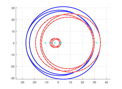
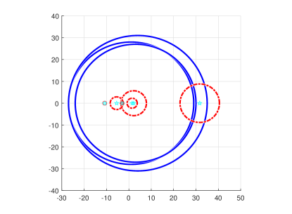
Figure 3: The Gershgorin discs (represented by the blue solid lines), obtained by Theorem $5.2$ given in [6], are compared with the Gershgorin discs derived from 3.1 presented in this paper (represented by the red dash-dot lines) under two similarity transformations for 3.1. (Left: $X=I$; Right: $X$ is a specifically selected transformation)

Example 3.1.

Let $\mathcal{A}\in\mathbb{R}^{3\times 3\times 2}$. Its frontal slices are $A_{1}$ and $A_{2}$, with their entries being

$$A_{1}=\left(\begin{array}[]{ccc}3&7&6\\ 4&1&9\\ 5&9&4\\ \end{array}\right),A_{2}=\left(\begin{array}[]{ccc}5&7&2\\ 1&4&10\\ 2&9&6\\ \end{array}\right).$$

By Theorem $5.2$ given in [6], we can draw the Gershgorin discs that contain all T-eigenvalues of tensor $\mathcal{A}$. The corresponding results, depicted by blue solid lines, visually represented in Figure 3.

To illustrate the Gershgorin discs generated by our presented result (referred to as 3.1), we employ two distinct similarity transformations. Initially, the matrix $\operatorname{bcirc}(\mathcal{A})$ is block-diagonalized using the normalized discrete Fourier transform matrix. And we choose the transformation matrix $X$ to be the identity matrix, denoted as $X=I_{mn}$, where $m=3$ and $n=2$. Then

$$I_{mn}^{-1}(F_{n}^{\mathrm{H}}\otimes I_{m})\operatorname{bcirc}(\mathcal{A})(F_{n}\otimes I_{m})I_{mn}=D+F:=M=\left(\begin{array}[]{cc}M_{1}&O\\ O&M_{2}\\ \end{array}\right),$$

where $O$ corresponds to the $3\times 3$ zero matrix.

The Gershgorin discs, defined by (3.4), are depicted in the left picture of Figure 3 as red dash-dot circles. Notably, these red dash-dot circles are contained within the blue solid circles, signifying a tighter bound compared to the result presented in [6]. Subsequently, we endeavor to seek smaller Gershgorin discs by designing a new transformation $X_{\text{new}}$. We apply Schur triangularization to matrices $M_{1}$ and $M_{2}$. Let $M_{i}=S_{i}T_{i}S_{i}^{-1},i=1,2.$ Set

$$X_{new}=\left(\begin{array}[]{cc}S_{1}&O\\ O&S_{2}\\ \end{array}\right).$$

Then we get

$$X_{new}^{-1}(F_{n}^{\mathrm{H}}\otimes I_{m})\operatorname{bcirc}(\mathcal{A})(F_{n}\otimes I_{m})X_{new}=D_{new}+F_{new},$$

in which we adopt the similar notations as presented in 3.1. In this case, $F_{\text{new}}$ is an upper quasi-triangular matrix that contains more zero entries than $F$. By applying the criterion (3.4) once again, we establish new Gershgorin circles, displayed in the right picture of Figure 3. Evidently, the new red dash-dot circles are significantly smaller than the blue solid ones.

In both depictions within Figure 3, the cyan pentagrams represent true T-eigenvalues of $\mathcal{A}$. This observation highlights that opting for an appropriate transformation matrix can lead to tighter bounds or even yield the true T-eigenvalues. The result presented in [6] is characterized by its simplicity and conciseness, which consequently incurs less computational cost. However, this advantage comes at the cost of producing only rough approximations for the bounds. In contrast, our derived result permits the adjustment of the transformation matrix to achieve more precise outcomes, albeit at the expense of increased computational resources.

Remark 3.2.

Eigenvalue sensitivity analysis is a subject of particular interest to many researchers, especially in the context of the symmetric eigenproblem for real matrices, where orthogonal transformations are commonly employed. Notably, classical results such as the Gershgorin disk theorem and the perturbation result Wielandt-Hoffman theorem [13] for real symmetric matrices are well-established and widely recognized. However, it is important to note that these results are not directly applicable to the real third-order tensor case. The primary reason for this limitation is that the block-diagonalized matrix of a real symmetric tensor, obtained via the normalized discrete Fourier transform matrix, may not retain its symmetry property. Consider the symmetric tensor $\mathcal{A}$ with three frontal slices: $A_{1}=\begin{bmatrix}1&2;2&4\end{bmatrix}$, $A_{2}=\begin{bmatrix}5&6;7&8\end{bmatrix}$, and $A_{3}=\begin{bmatrix}5&7;6&8\end{bmatrix}$, represented in MATLAB notation. This serves as a meaningful illustrative example.

3.2 Bauer-Fike theorem for tensors

The Bauer-Fike theorem is a classical result for complex-valued diagonalizable matrices, dealing with eigenvalue perturbation theory. It provides an absolute upper bound for the deviation of a perturbed matrix eigenvalue from a chosen eigenvalue of the original matrix, estimated by the product of the condition number of the eigenvector matrix and the perturbation’s norm [1].

Extending the Bauer-Fike theorem to the case of non-diagonalizable matrices has been explored in [10, 13]. Moreover, the perturbation result depending on part of the spectra of a matrix with disjoint spectral sets was also considered in [10].

In this subsection, we first present a generalization of the renowned Bauer-Fike theorem, applicable not only to diagonalizable matrices but also to the third-order tensor case. Furthermore, we extend its general form to encompass non-diagonalizable matrices within the context of third-order tensors.

Before presenting the main results, we introduce the definitions of tensor-$p$ norms, following a similar formulation to the tensor spectral norm employed in tensor robust principal component analysis [27]. Additionally, we define the tensor condition number for simplicity. Let $\mathcal{A}\in\mathbb{C}^{m\times m\times n}$. The tensor-$p$ norm is defined as $\|\mathcal{A}\|_{p}:=\|\operatorname{bcirc}(\mathcal{A})\|_{p}$, and the condition number of $\mathcal{A}$ is denoted as $\kappa_{p}(\mathcal{A}):=\|\operatorname{bcirc}(\mathcal{A})\|_{p}\left\|\operatorname{bcirc}(\mathcal{A}^{-1})\right\|_{p}$.

Theorem 3.2 (Bauer-Fike theorem for tensors).

Let $\mathcal{A}\in\mathbb{C}^{m\times m\times n}$ be an F-diagonalizable tensor. This implies the existence of an invertible tensor $\mathcal{P}$ such that

$$\mathcal{P}^{-1}*\mathcal{A}*\mathcal{P}=\mathcal{D},$$ (3.5)

where $\mathcal{D}$ is an F-diagonal tensor. Assuming $\mu$ is a T-eigenvalue of $\mathcal{A}+\delta\mathcal{A}$, with $\delta$ being a small number and indicating a small perturbation on the original tensor $\mathcal{A}$. Then, considering the spectral norm or Frobenius norm cases, there exists a T-eigenvalue $\lambda$ of $\mathcal{A}$ such that:

$$|\lambda-\mu|\leq\kappa_{p}(\mathcal{P})\|\delta\mathcal{A}\|_{p},\ p=2,F.$$ (3.6)

Moreover, for the $1$- and $\infty$-norms, we have

$$|\lambda-\mu|\leq\kappa_{p}(\mathcal{P})\kappa_{p}(F_{n}\otimes I_{m})\|\delta\mathcal{A}\|_{p},\ p=1,\infty.$$ (3.7)

Proof.   By 2.1, we know that the equality (3.5) is equivalent to

$$(\operatorname{bcirc}(\mathcal{P}))^{-1}\operatorname{bcirc}(\mathcal{A})\operatorname{bcirc}(\mathcal{P})=\operatorname{bcirc}(\mathcal{D}).$$

Since the right-hand side of the above equality is a block circulant matrix, thus it can be block-diagonalized by the normalized discrete Fourier transform matrix. Then we have

$$(F_{n}^{\mathrm{H}}\otimes I_{m})\operatorname{bcirc}(\mathcal{D})(F_{n}\otimes I_{m})=D=\left[\begin{array}[]{cccc}{D^{(1)}}&{}\hfil&{}\hfil&{}\hfil\\ {}\hfil&{D^{(2)}}&{}\hfil&{}\hfil\\ {}\hfil&{}\hfil&{\ddots}&{}\hfil\\ {}\hfil&{}\hfil&{}\hfil&{D^{(n)}}\end{array}\right].$$

By 2.3, we can see that $D^{(1)},D^{(2)},\ldots,D^{(n)}$ are diagonal matrices since $\mathcal{D}$ is an F-diagonal tensor. Let $X=\operatorname{bcirc}(\mathcal{P})(\kappa_{p}(\mathcal{A}))$. Then we get $X^{-1}\operatorname{bcirc}(\mathcal{A})X=D$. Hence by Bauer-Fike theorem [13], there is an eigenvalue $\lambda$ of bcirc(A), hence a T-eigenvalue $\lambda$ of $\mathcal{A}$, such that

$$|\lambda-\mu| \leq\|X^{-1}\|\|X\|\|\operatorname{bcirc}(\delta\mathcal{A})\|$$

$$\leq\kappa_{p}(\mathcal{P})\kappa_{p}(F_{n}\otimes I_{m})\|\delta\mathcal{A}\|_{p}.$$

Under the $2$-norm case, since $F_{n}\otimes I_{m}$ and $F_{n}^{\mathrm{H}}\otimes I_{m}$ are unitary, then

$$\kappa_{2}(F_{n}\otimes I_{m})=\|F_{n}\otimes I_{m}\|_{2}\|F_{n}^{\mathrm{H}}\otimes I_{m}\|_{2}=1,$$

and we obtain the inequality (3.6). The result for the Frobenius norm follows trivially from the definitions presented earlier, as the spectral norm of tensor $\mathcal{A}$ is not greater than its Frobenius norm. The proof is completed. ∎

Remark 3.3.

At the same time, Theorem 5.3 in [6] has also addressed the Bauer-Fike theorem. The theorem states that under certain conditions, the inequality $|\lambda-\mu|\leq\|\mathcal{P}^{-1}\|_{2}\|\mathcal{P}\|_{2}\|\mathcal{A}-\mathcal{B}\|_{2}$ holds. It is evident that this is a specific case of the result presented above, applicable only to the $2$-norm case.

The following conclusion describes the relationship between the variation of T-spectra, i.e., the collection of all T-eigenvalues, and the difference of two tensors. We omit the proof, as it can be easily obtained using the above theorem.

Corollary 3.1.

Let $\mathcal{A},\mathcal{B}\in\mathbb{C}^{m\times m\times n}$. $\mathcal{A}$ is an F-diagonalizable tensor with decomposition as

$$\mathcal{P}^{-1}*\mathcal{A}*\mathcal{P}=\mathcal{D}.$$

Let $s_{\mathcal{A}}(\mathcal{B})$ be the distance of two T-spectral sets $\Lambda_{\mathcal{A}}=\{\lambda_{i}\}_{i=1}^{mn}$ and $\Lambda_{\mathcal{B}}=\{\mu_{i}\}_{i=1}^{mn}$. That is,

$$s_{\mathcal{A}}(\mathcal{B})=\max_{1\leq j\leq mn}\{\min_{1\leq i\leq mn}|\lambda_{i}-\mu_{j}|\}.$$

Then the following conclusion holds,

$$s_{\mathcal{A}}(\mathcal{B})\leq\kappa_{2}(\mathcal{P})\|\mathcal{B}-\mathcal{A}\|_{2}.$$

Moreover, if $\mathcal{A}$ is a normal tensor, then

$$s_{\mathcal{A}}(\mathcal{B})\leq\|\mathcal{B}-\mathcal{A}\|_{2}.$$

In general, most third-order tensors are not F-diagonalizable, which implies that (3.5) is usually not satisfied for a given tensor. Therefore, we cannot obtain an F-diagonal tensor through tensor-tensor multiplication by an invertible tensor. In such cases, we resort to the following decomposition.

Lemma 3.1.

([19, 28, 32], T-Schur decomposition). Let $\mathcal{A}\in\mathbb{C}^{m\times m\times n}$. Then there exists a unitary tensor $\mathcal{Q}$ such that

$$\mathcal{Q}^{-1}*\mathcal{A}*\mathcal{Q}=\mathcal{T}=\mathcal{D}+\mathcal{N},$$ (3.8)

where $\mathcal{D}$ is an F-diagonal tensor, and each frontal slice of $\mathcal{N}$ is strictly upper triangular.

In the following, we present two general cases of the Bauer-Fike theorem for tensors (i.e., 3.2). These theorems are based on the T-Schur decomposition and can be regarded as generalizations of the Bauer-Fike theorems for non-diagonalizable matrices given in [10, 13]. To ensure completeness, we provide a detailed proof for one of the cases.

Theorem 3.3.

(Generalization of Bauer-Fike theorem for tensors I). Let $\mathcal{Q}^{-1}*\mathcal{A}*\mathcal{Q}=\mathcal{D}+\mathcal{N}$ be a T-Schur decomposition of $\mathcal{A}\in\mathbb{C}^{m\times m\times n}$. Given $\mathcal{B}\in\mathbb{C}^{m\times m\times n}$ and $\varepsilon$ as a small scalar, suppose $\mu$ is a T-eigenvalue of $\mathcal{A}+\varepsilon\mathcal{B}$, and let $q$ be the smallest positive number such that $|N|^{q}=0$, in which

$$N:=\left[\begin{array}[]{llll}N^{(1)}&&&\\ &N^{(2)}&&\\ &&\ddots&\\ &&&N^{(n)}\end{array}\right]=(F_{n}^{\mathrm{H}}\otimes I_{m})\operatorname{bcirc}(\mathcal{N})(F_{n}\otimes I_{m}),$$

and $|N|=(|N_{ij}|)$ denotes the absolute of a matrix element-wisely. Then, for the spectral and Frobenius norms, we establish the following bounds:

$$\min_{\lambda\in\Lambda(\mathcal{A})}|\lambda-\mu|\leq\max\left\{\theta,\theta^{1/q}\right\},$$ (3.9)

in which

$$\theta=\|\varepsilon\mathcal{B}\|_{p}\sum_{k=0}^{q-1}\|N\|_{p}^{k},\ p=2,F.$$ (3.10)

Additionally, for the $1$- and $\infty$-norms, the bounds are given by:

$$\min_{\lambda\in\Lambda(\mathcal{A})}|\lambda-\mu|\leq\max\{\theta_{p},\theta_{p}^{1/q}\},$$ (3.11)

where

$$\theta_{p}=\|\varepsilon\mathcal{B}\|_{p}\kappa_{p}(\mathcal{Q})\kappa_{p}(F_{n}\otimes I_{m})\sum_{k=0}^{q-1}\|N\|_{2}^{k},\ p=1,\infty.$$

Proof.   The theorem is evident when $\mu\in\Lambda(\mathcal{A})$, as the left-hand sides of (3.9) and (3.11) vanish. Therefore, we assume that $\mu\notin\Lambda(\mathcal{A})$. By 2.1, we can see that

$$\mu I_{mn}-\operatorname{bcirc}(\mathcal{A}+\varepsilon\mathcal{B})=\mu I_{mn}-\operatorname{bcirc}(\mathcal{A})-\operatorname{bcirc}(\varepsilon\mathcal{B}),$$

and moreover $\mu I_{mn}-\operatorname{bcirc}(\mathcal{A}+\varepsilon\mathcal{B})$ is singular. This means that

$$(F_{n}^{\mathrm{H}}\otimes I_{m})\operatorname{bcirc}(\mathcal{Q})^{-1}[\mu I_{mn}-\operatorname{bcirc}(\mathcal{A})-\operatorname{bcirc}(\varepsilon\mathcal{B})]\operatorname{bcirc}(\mathcal{Q})(F_{n}\otimes I_{m})$$ (3.12)

is also singular since the matrices multiplied on the left and right sides are nonsingular. Notice that

$$(F_{n}^{\mathrm{H}}\otimes I_{m})\operatorname{bcirc}(\mathcal{Q})^{-1}\operatorname{bcirc}(\mathcal{A})\operatorname{bcirc}(\mathcal{Q})(F_{n}\otimes I_{m})$$

$$= (F_{n}^{\mathrm{H}}\otimes I_{m})[\operatorname{bcirc}(\mathcal{D})+\operatorname{bcirc}(\mathcal{N})](F_{n}\otimes I_{m})$$

$$= \left[\begin{array}[]{llll}D^{(1)}&&&\\ &D^{(2)}&&\\ &&\ddots&\\ &&&D^{(n)}\end{array}\right]+\left[\begin{array}[]{llll}N^{(1)}&&&\\ &N^{(2)}&&\\ &&\ddots&\\ &&&N^{(n)}\end{array}\right]$$

$$:= D+N.$$

Therefore (3.12) can be rewritten as

$$\mu I_{mn}-D-N-(F_{n}^{\mathrm{H}}\otimes I_{m})\operatorname{bcirc}(\mathcal{Q})^{-1}\operatorname{bcirc}(\varepsilon\mathcal{B})\operatorname{bcirc}(\mathcal{Q})(F_{n}\otimes I_{m}),$$

and thus the following matrix

$$I_{mn}-(\mu I_{mn}-D-N)^{-1}(F_{n}^{\mathrm{H}}\otimes I_{m})\operatorname{bcirc}(\mathcal{Q})^{-1}\operatorname{bcirc}(\varepsilon\mathcal{B})\operatorname{bcirc}(\mathcal{Q})(F_{n}\otimes I_{m})$$ (3.13)

is singular.

By the assumption that $|N|^{q}=0$ and note that $\mu I_{mn}-D$ is a nonsingular diagonal matrix, it follows that $((\mu I_{mn}-D)^{-1}N)^{q}=0$. Hence,

$$((\mu I_{mn}-D)-N)^{-1}=\sum_{k=0}^{q-1}\left((\mu I_{mn}-D)^{-1}N\right)^{k}(\mu I_{mn}-D)^{-1},$$

and

$$\|((\mu I_{mn}-D)-N)^{-1}\|\leq\frac{1}{\min_{\lambda\in\Lambda(\mathcal{A})}|\lambda-\mu|}\sum_{k=0}^{q-1}\left(\frac{\|N\|}{\min_{\lambda\in\Lambda(\mathcal{A})}|\lambda-\mu|}\right)^{k}$$

holds under the $1$-, $2$- and $\infty$-norms cases.

If $\min_{\lambda\in\Lambda(\mathcal{A})}|\lambda-\mu|\geq 1$, then

$$\|((\mu I_{mn}-D)-N)^{-1}\|\leq\frac{1}{\min_{\lambda\in\Lambda(\mathcal{A})}|\lambda-\mu|}\sum_{k=0}^{q-1}\|N\|^{k}.$$

In the case of $\min_{\lambda\in\Lambda(\mathcal{A})}|\lambda-\mu|<1$, then

$$\|((\mu I_{mn}-D)-N)^{-1}\|\leq\frac{1}{(\min_{\lambda\in\Lambda(\mathcal{A})}|\lambda-\mu|)^{q}}\sum_{k=0}^{q-1}\|N\|^{k}.$$

By (3.13), we can obtain

$$1 \leq\left\|(\mu I_{mn}-D-N)^{-1}(F_{n}^{\mathrm{H}}\otimes I_{m})\cdot\operatorname{bcirc}(\mathcal{Q})^{-1}\operatorname{bcirc}(\varepsilon\mathcal{B})\operatorname{bcirc}(\mathcal{Q})\cdot(F_{n}\otimes I_{m})\right\|$$

$$=\left\|(\mu I_{mn}-D-N)^{-1}\right\|\|\operatorname{bcirc}(\varepsilon\mathcal{B})\|\|F_{n}^{\mathrm{H}}\otimes I_{m}\|\|F_{n}\otimes I_{m}\|\|\operatorname{bcirc}(\mathcal{Q})^{-1}\|\|\operatorname{bcirc}(\mathcal{Q})\|.$$

Combining the above theoretical analyses, in the spectral norm case, we can see

$$\min_{\lambda\in\Lambda(\mathcal{A})}|\lambda-\mu|\leq\|\operatorname{bcirc}(\varepsilon\mathcal{B})\|_{2}\sum_{k=0}^{q-1}\|N\|_{2}^{k}\quad\text{or }\quad(\min_{\lambda\in\Lambda(\mathcal{A})}|\lambda-\mu|)^{q}\leq\|\operatorname{bcirc}(\varepsilon\mathcal{B})\|_{2}\sum_{k=0}^{q-1}\|N\|_{2}^{k}$$

for

$$\min_{\lambda\in\Lambda(\mathcal{A})}|\lambda-\mu|\geq 1\quad\text{or }\quad\min_{\lambda\in\Lambda(\mathcal{A})}|\lambda-\mu|<1,$$

respectively. Let $\theta=\|\operatorname{bcirc}(\varepsilon\mathcal{B})\|_{2}\sum_{k=0}^{q-1}\|N\|_{2}^{k}$. Then we get the result (3.9) for the spectral norm. Similar to the proof given in 3.2, the Frobenius norm case can be obtained easily.

For the $1$- and $\infty$-norms, by using (3.13) again we get

$$\min_{\lambda\in\Lambda(\mathcal{A})}|\lambda-\mu|\leq\max\{\theta_{p},\theta_{p}^{1/q}\},$$

where

$$\theta_{p}=\|\operatorname{bcirc}(\varepsilon\mathcal{B})\|_{p}\kappa_{p}(\mathcal{Q})\kappa_{p}(F_{n}\otimes I_{m})\sum_{k=0}^{q-1}\|N\|_{2}^{k}.$$

The proof is completed. ∎

We now present a more generalized result of 3.2. In contrast to the previous theorem, which involves an F-diagonal tensor, the following result considers the block-diagonal case.

Let $\mathcal{A}\in\mathbb{C}^{m\times m\times n}$. Notice that $\operatorname{bcirc}(\mathcal{A})$ can be block-diagonalized as follows,

$$(F_{n}^{\mathrm{H}}\otimes I_{m})\operatorname{bcirc}(\mathcal{A})(F_{n}\otimes I_{m})=\left[\begin{array}[]{cccc}{A^{(1)}}&{}\hfil&{}\hfil&{}\hfil\\ {}\hfil&{A^{(2)}}&{}\hfil&{}\hfil\\ {}\hfil&{}\hfil&{\ddots}&{}\hfil\\ {}\hfil&{}\hfil&{}\hfil&{A^{(n)}}\end{array}\right].$$

By 2.3, we know that $A^{(i)}$ where $i=1,\ldots,n$ may not diagonal since generally tensor $\mathcal{A}$ is not F-diagonal. For each matrix $A^{(i)}$, suppose $X^{(i)}$ is a transformation matrix such that $(X^{(i)})^{-1}A^{(i)}X^{(i)}=\operatorname{diag}(A^{(i)}_{k_{i}})$ where $A^{(i)}_{k_{i}}$ is in triangular Schur form with

$$A^{(i)}_{k_{i}}=D^{(i)}_{k_{i}}+N^{(i)}_{k_{i}},\ k_{i}=1,\ldots,\ell_{i},$$

in which $D^{(i)}_{k_{i}}$ is diagonal for each $i$. Denote $\operatorname{bcirc}(\mathcal{X})=(F_{n}\otimes I_{m})\operatorname{diag}(X^{(1)},X^{(2)},\ldots,X^{(n)})(F_{n}^{\mathrm{H}}\otimes I_{m})$. Then we get

$$(F_{n}^{\mathrm{H}}\otimes I_{m})\operatorname{bcirc}(\mathcal{X})^{-1}\operatorname{bcirc}(\mathcal{A})\operatorname{bcirc}(\mathcal{X})(F_{n}\otimes I_{m})$$

$$= \left[\begin{array}[]{llll}\operatorname{diag}(A^{(1)}_{k_{1}})&&&\\ &\operatorname{diag}(A^{(2)}_{k_{2}})&&\\ &&\ddots&\\ &&&\operatorname{diag}(A^{(n)}_{k_{n}})\end{array}\right]=\left[\begin{array}[]{ccccccc}A_{1}^{(1)}&&&&&&\\ &\ddots&&&&&\\ &&A_{\ell_{1}}^{(1)}&&&&\\ &&&\ddots&&&\\ &&&&A_{1}^{(n)}&&\\ &&&&&\ddots&\\ &&&&&&A_{\ell_{n}}^{(n)}\end{array}\right]$$

$$= \left[\begin{array}[]{ccccccc}D_{1}^{(1)}&&&&&&\\ &\ddots&&&&&\\ &&D_{\ell_{1}}^{(1)}&&&&\\ &&&\ddots&&&\\ &&&&D_{1}^{(n)}&&\\ &&&&&\ddots&\\ &&&&&&D_{\ell_{n}}^{(n)}\end{array}\right]+\left[\begin{array}[]{ccccccc}N_{1}^{(1)}&&&&&&\\ &\ddots&&&&&\\ &&N_{\ell_{1}}^{(1)}&&&&\\ &&&\ddots&&&\\ &&&&N_{1}^{(n)}&&\\ &&&&&\ddots&\\ &&&&&&N_{\ell_{n}}^{(n)}\end{array}\right]$$

$$:= \tilde{D}+\tilde{N}.$$

By the above analysis, we have the following conclusion.

Theorem 3.4.

(Generalization of Bauer-Fike theorem for tensors II). If $\mu$ is a T-eigenvalue of $\mathcal{A}+\varepsilon\mathcal{B}$ and $q$ is the dimension of $A_{k_{i}}^{(i)}$, then we have

$$\min_{\lambda\in\Lambda(\mathcal{A})}|\lambda-\mu|\leq\max\left\{\theta_{1},\theta_{1}^{1/q}\right\},$$

where

$$\theta_{1}=C\varepsilon\|\mathcal{B}\|_{p}\kappa_{p}(\mathcal{X}),\ p=2,F.$$

and $C=\sum_{k=0}^{q-1}\|N^{i}\|_{2}^{k}$ provided that $\max_{j}\left\|\left(A^{(i)}_{j}-\mu I\right)^{-1}\right\|$ occurring at $j=k_{i}$.

For $1$- and $\infty$-norms, under the above condition, we get

$$\min_{\lambda\in\Lambda(\mathcal{A})}|\lambda-\mu|\leq\max\{\theta_{2},\theta_{2}^{1/q}\},$$

where

$$\theta_{2}=C\varepsilon\|\mathcal{B}\|_{p}\kappa_{p}(\mathcal{X})\kappa_{p}(F_{n}\otimes I_{m}),\ p=1,\infty.$$

Proof.   We only need to consider the case that $\mu$ is not a T-eigenvalue of $\mathcal{A}$. Hence $\mu I_{mn}-\tilde{D}-\tilde{N}$ is nonsingular. Similar as (3.13), the matrix

$$I_{mn}-(\mu I_{mn}-\tilde{D}-\tilde{N})^{-1}(F_{n}\otimes I_{m})\operatorname{bcirc}(\mathcal{X})^{-1}\operatorname{bcirc}(\varepsilon\mathcal{B})\operatorname{bcirc}(\mathcal{X})(F_{n}^{\mathrm{H}}\otimes I_{m})$$

is singular. By using a similar proof process given in 3.3, we could get the conclusion. ∎

3.3 Kahan theorem for tensors

The perturbation of a Hermite tensor by another Hermite tensor is studied in [24, Theorem 4.1]. In the following, we present a result involving the perturbation of a Hermite tensor by any tensors.

Theorem 3.5.

(Kahan theorem for tensors). Let $\mathcal{A}\in\mathbb{R}^{m\times m\times n}$ be a Hermite tensor. Suppose that its T-spectral set is denoted as $\Lambda_{\mathcal{A}}=\{\lambda_{i}\}_{i=1}^{mn}$ such that its T-eigenvalues are arranged in a non-increasing order:

$$\lambda_{\max}=\lambda_{1}\geq\lambda_{2}\geq\cdots\geq\lambda_{mn-1}\geq\lambda_{mn}=\lambda_{\min}.$$ (3.14)

Suppose that $\mathcal{B}=\mathcal{A}+\mathcal{E}$ and let $\Lambda_{\mathcal{B}}=\{\beta_{k}+i\gamma_{k}\}_{k=1}^{mn}$ such that $\beta_{1}\geq\beta_{2}\geq\cdots\geq\beta_{mn-1}\geq\beta_{mn}.$ Let

$$E_{y}=\frac{\operatorname{bcirc}(\mathcal{E})-\operatorname{bcirc}(\mathcal{E})^{\mathrm{H}}}{2i}$$

and

$$\sigma_{k}=\{\beta+i\gamma\in\mathbb{C}:|\beta+i\gamma-\lambda_{k}|\leq\|\mathcal{E}\|_{2},|\gamma|\leq\|E_{y}\|_{2}\}.$$

Then

$$\Lambda_{\mathcal{B}}\subset\bigcup_{k=1}^{mn}\sigma_{k}.$$

Proof.   On one hand, as stated in 2.4, a Hermite tensor can be F-diagonalized by a unitary tensor. According to 3.1, there exists a T-eigenvalue $\lambda_{k}$ such that $|\beta+i\gamma-\lambda_{k}|\leq\|\mathcal{E}\|_{2}$ for any given T-eigenvalue $\beta+i\gamma$ of $\mathcal{B}$.

On the other hand, suppose that $\mathcal{B}*\mathcal{X}=(\beta+i\gamma)\mathcal{X}$, then by the definition of tensor-tensor multiplication, it is equivalent to

$$\operatorname{bcirc}(\mathcal{B})\operatorname{unfold}(\mathcal{X})=(\beta+i\gamma)\operatorname{unfold}(\mathcal{X}).$$

Thus, it is reasonable to assume that $\|\operatorname{unfold}(\mathcal{X})\|_{2}=1$, since $\mathcal{X}$ is nonzero, which implies that the vector $\operatorname{unfold}(\mathcal{X})$ is also nonzero. Therefore,

$$(\operatorname{unfold}(\mathcal{X}))^{\mathrm{H}}\operatorname{bcirc}(\mathcal{B})\operatorname{unfold}(\mathcal{X})=\beta+i\gamma\quad\text{and}\quad(\operatorname{unfold}(\mathcal{X}))^{\mathrm{H}}\operatorname{bcirc}(\mathcal{B})^{\mathrm{H}}\operatorname{unfold}(\mathcal{X})=\beta-i\gamma,$$

which implies that

$$\gamma=\frac{(\operatorname{unfold}(\mathcal{X}))^{\mathrm{H}}[\operatorname{bcirc}(\mathcal{B})-\operatorname{bcirc}(\mathcal{B})^{\mathrm{H}}]\operatorname{unfold}(\mathcal{X})}{2i}=\operatorname{unfold}(\mathcal{X}))^{\mathrm{H}}E_{y}\operatorname{unfold}(\mathcal{X}).$$

Thus $|\gamma|\leq\|E_{y}\|_{2}$.

The conclusion can be obtained from the combination of these two parts. ∎

4 Pseudospectra of third-order tensors

The pseudospectra of finite-dimensional matrices and their extension to linear operators in Banach space have been extensively investigated and summarized in the classical book by Trefethen and Embree [47]. In the book, four different definitions of matrix pseudospectra are introduced and shown to be equivalent under certain conditions. Properties of pseudospectra are also collected, and a characterization of the pseudospectra for normal matrices is provided. Additionally, for diagonalizable but not necessarily normal matrices, the corresponding Bauer-Fike theorem is presented, which can be found in [47, Theorems 2.2, 2.3, and 2.4]. The book also covers various methods for computing matrix pseudospectra; for more details, refer to [47, Section 39]. Notably, the book [47] includes representative numerical results, including plots of pseudospectra that span nearly every section of the book.

Before presenting our own results, we review the definitions of pseudospectra for the matrix case.

Definition 4.1.

([47, Section 2]). Let $A\in\mathbb{C}^{m\times m}$ and $\varepsilon>0$ be arbitrary. $\lambda(A)$ is the set of eigenvalues of $A$, and the convention $\|(zI-A)^{-1}\|=\infty$ for $z\in\lambda(A)$ is employed.
(I) The $\varepsilon$-pseudospectra $\lambda_{\varepsilon}(A)$ of $A$ is the set of $z\in\mathbb{C}$ such that $\|(zI-A)^{-1}\|>\varepsilon^{-1}$.
(II) The $\varepsilon$-pseudospectra $\lambda_{\varepsilon}(A)$ of $A$ is the set of $z\in\mathbb{C}$ such that $z\in\lambda(A+E)$ for some $E\in\mathbb{C}^{m\times m}$ with $\|E\|<\varepsilon$.
(III) The $\varepsilon$-pseudospectra $\lambda_{\varepsilon}(A)$ of $A$ is the set of $z\in\mathbb{C}$ such that $\|(zI-A)\mathbf{v}\|<\varepsilon$ for some $v\in\mathbb{C}^{m}$ with $\|\mathbf{v}\|=1$.
(IV) For $\|\cdot\|=\|\cdot\|_{2}$, $\lambda_{\varepsilon}(A)$ is the set of $z\in\mathbb{C}$ such that $\sigma_{min}(zI-A)<\varepsilon$ where $\sigma_{min}(\cdot)$ denotes the minimum singular value.

Remark 4.1.

For any matrix $A\in\mathbb{C}^{m\times m}$, the equivalence of the three definitions (I), (II), and (III) given in 4.1 has been established. Moreover, when the spectral norm is chosen, definition (IV) is shown to be equivalent to the other three characterizations of matrix pseudospectra [47].

In this section, we delve into the study of pseudospectra for third-order tensors within the tensor-tensor multiplication framework. Specifically, we explore different formulations of pseudospectra for third-order tensors in Subsection 4.1. Subsection 4.2 is dedicated to the examination of various properties of pseudospectra related to third-order tensors. Finally, in Subsection 4.3, we present plots illustrating the computed results of $\varepsilon$-pseudospectra for given tensors.

4.1 Pseudospectra of third-order tensors under tensor-tensor multiplication

Various definitions on $\varepsilon$-pseudospectra of $m\times m\times n$ tensors are studied in this subsection. If the norm $\|\cdot\|$ is not specified, we adopt the convention that it corresponds to the $p$ norm, where $p=1,2,\infty.$

Definition 4.2 ($\varepsilon$-pseudospectra of tensors).

Let $\mathcal{A}\in\mathbb{C}^{m\times m\times n}$. Then the block circulant matrix $\operatorname{bcirc}(\mathcal{A})$ generated by tensor $\mathcal{A}$ can be factored as follows,

$$\operatorname{bcirc}(\mathcal{A})=\left(F_{n}\otimes I_{m}\right)\left[\begin{array}[]{cccc}{A^{(1)}}&{}\hfil&{}\hfil&{}\hfil\\ {}\hfil&{A^{(2)}}&{}\hfil&{}\hfil\\ {}\hfil&{}\hfil&{\ddots}&{}\hfil\\ {}\hfil&{}\hfil&{}\hfil&{A^{(n)}}\end{array}\right]\left(F_{n}^{\mathrm{H}}\otimes I_{m}\right).$$ (4.1)

For each matrix $A^{(i)}\in\mathbb{C}^{m\times m}$ where $i\in[n]:=\{1,\ldots,n\}$, we have

$$\lambda_{\varepsilon}(A^{(i)}):=\left\{z\in\mathbb{C}:\left\|(zI_{m}-A^{(i)})^{-1}\right\|>\varepsilon^{-1}\right\},$$

where $\varepsilon$ is an arbitrary positive scalar. If there are some $i$ such that $zI_{m}-A^{(i)}$ are singular for $z\in\lambda(A^{(i)})$, we define $\left\|(zI_{m}-A^{(i)})^{-1}\right\|=\infty$.

In this definition, we denote the block diagonal matrix in (4.1) as $\operatorname{diag}(A^{(1)},\ldots,A^{(n)}):=A$ and its spectrum is $\Lambda(A)$.

(I) We call

$$\Lambda_{\varepsilon}(\mathcal{A}):=\left\{z\in\mathbb{C}:\max_{i\in[n]}\left\|(zI_{m}-A^{(i)})^{-1}\right\|>\varepsilon^{-1}\right\}$$

as the $\varepsilon$-pseudospectra of tensor $\mathcal{A}$.

(II) $\Lambda_{\varepsilon}(\mathcal{A})=\{z\in\mathbb{C}:z\in\Lambda(A+E)$ for some $E\in\mathbb{C}^{mn\times mn}$ with $\|E\|<\varepsilon\}.$

(III) $\Lambda_{\varepsilon}(\mathcal{A})=\left\{z\in\mathbb{C}:\right.$ There exists $v\in\mathbb{C}^{mn}$ with $\|v\|=1$ such that $\left.\|(A-zI_{mn})v\|<\varepsilon\right\}.$

Theorem 4.1.

The three different characterizations (I), (II), and (III) on $\varepsilon$-pseudospectra of third-order tensors are equivalent.

Proof.   For a block diagonal matrix, we find that $\|A\|=\max_{i\in[n]}\|A^{(i)}\|$, and the inverse of $A$ can be obtained by computing the inverse of each $A^{(i)}$. Therefore, we have

$$\max_{i\in[n]}\left\|(zI_{m}-A^{(i)})^{-1}\right\|=\left\|(zI_{mn}-A)^{-1}\right\|,$$

and consequently,

$$\Lambda_{\varepsilon}(\mathcal{A})=\left\{z\in\mathbb{C}:\left\|(zI_{mn}-A)^{-1}\right\|>\varepsilon^{-1}\right\}.$$ (4.2)

The equivalence of (4.2) with (II) and (III) can be easily deduced from 4.1. ∎

Remark 4.2.

Notice that $z\in\mathbb{C}$ and is a variable, while $A^{(i)}$ is stationary when the tensor $\mathcal{A}$ is given. Therefore, by (I) in 4.2, we can also see that

$$\Lambda_{\varepsilon}(\mathcal{A})=\bigcup_{i=1}^{n}\Lambda_{\varepsilon}(A^{(i)})=\bigcup_{i=1}^{n}\left\{z\in\mathbb{C}:\left\|(zI_{m}-A^{(i)})^{-1}\right\|>\varepsilon^{-1}\right\}.$$

In the case of the spectral norm, we provide the following definition.

Definition 4.3.

Let $\mathcal{A}\in\mathbb{C}^{m\times m\times n}$. Then the block-circulant matrix $\operatorname{bcirc}(\mathcal{A})$ generated by the tensor $\mathcal{A}$ can be factored as shown in (4.1). For each square matrix $A^{(i)}$, where $i\in[n]$, we have

$$\Lambda_{\varepsilon}(A^{(i)})=\left\{z\in\mathbb{C}:\sigma_{\min}(zI_{m}-A^{(i)})\leq\varepsilon\right\},$$

where $\varepsilon$ is a positive scalar and $\sigma_{min}(\cdot)$ denotes the minimum singular value. We refer to

$$\Lambda_{\varepsilon}(\mathcal{A})=\bigcup_{i=1}^{n}\Lambda_{\varepsilon}(A^{(i)})$$

as the $\varepsilon$-pseudospectra of tensor $\mathcal{A}$.

By 4.2, we get the following conclusion.

Theorem 4.2.

In the case of the spectral norm, the characterization given in 4.3 is equivalent to the three characterizations (I), (II), and (III) given in 4.2.

4.2 Properties of pseudospectra of tensors

In this subsection, we investigate the properties of pseudospectra for third-order tensors. Several fundamental results are presented in the following theorem.

Theorem 4.3.

Let $\mathcal{A}\in\mathbb{C}^{m\times m\times n}$ and consider an arbitrary positive scalar $\varepsilon$. The following properties hold for the pseudospectra $\Lambda_{\varepsilon}(\mathcal{A})$:

(I) The set $\Lambda_{\varepsilon}(\mathcal{A})$ is nonempty, open, and bounded. Moreover, there are at most $nm$ connected components, each containing one or more T-eigenvalues of $\mathcal{A}$.

(II) For any $c\in\mathbb{C}$, we have $\Lambda_{\varepsilon}(\mathcal{A}+c)=c+\Lambda_{\varepsilon}(\mathcal{A})$, where $\mathcal{A}+c$ is shorthand for $\mathcal{A}+c\mathcal{E}$, and $\mathcal{E}$ is the identity tensor with the same size as $\mathcal{A}$.

(III) For any nonzero $c\in\mathbb{C}$, we have $\Lambda_{|c|\varepsilon}(c\mathcal{A})=c\Lambda_{\varepsilon}(\mathcal{A})$.

(IV) If the spectral norm is applied, then $\Lambda_{\varepsilon}\left(\mathcal{A}^{\mathrm{H}}\right)=\overline{\Lambda_{\varepsilon}(\mathcal{A})}$.

Proof.   To prove the assertion of (I), we utilize (4.1) and 4.2, which allow us to exploit the properties of $\Lambda_{\varepsilon}(A^{(i)})$ for each matrix $A^{(i)}$. It is well-known that $\Lambda_{\varepsilon}(A^{(i)})$ is nonempty, open, and bounded, with at most $m$ connected components, each containing one or more eigenvalues of $A^{(i)}$ [47, Theorem 2.4]. Consequently, these same properties also hold for the given tensor $\mathcal{A}$ by the above analysis. Additionally, the number of connected components is bounded by $nm$ due to the relationship expressed by

$$\Lambda_{\varepsilon}(\mathcal{A})=\bigcup_{i=1}^{n}\Lambda_{\varepsilon}(A^{(i)}).$$

Now, we proceed to part (II). Denote $\left(F_{n}^{\mathrm{H}}\otimes I_{m}\right)\operatorname{bcirc}(\mathcal{A})\left(F_{n}\otimes I_{m}\right):=A$. First, note that

$$\operatorname{bcirc}(\mathcal{A}+c\mathcal{E}) =\left[\begin{array}[]{ccccc}{A_{1}+cI_{m}}&{A_{n}}&{A_{n-1}}&{\cdots}&{A_{2}}\\ {A_{2}}&{A_{1}+cI_{m}}&{A_{n}}&{\cdots}&{A_{3}}\\ {\vdots}&{\ddots}&{\ddots}&{\ddots}&{\vdots}\\ {A_{n}}&{A_{n-1}}&{\ddots}&{A_{2}}&{A_{1}+cI_{m}}\end{array}\right]$$

$$=\operatorname{bcirc}(\mathcal{A})+c\operatorname{bcirc}(\mathcal{E})$$

$$=\left(F_{n}\otimes I_{m}\right)A\left(F_{m}^{\mathrm{H}}\otimes I_{n}\right)+c[\left(F_{m}\otimes I_{n}\right)I_{mn}\left(F_{m}^{\mathrm{H}}\otimes I_{n}\right)]$$

$$=\left(F_{n}\otimes I_{m}\right)(A+cI_{mn})\left(F_{n}^{\mathrm{H}}\otimes I_{m}\right)$$

$$=\left(F_{n}\otimes I_{m}\right)\left[\begin{array}[]{cccc}{A^{(1)}+cI_{m}}&{}\hfil&{}\hfil&{}\hfil\\ {}\hfil&{A^{(2)}+cI_{m}}&{}\hfil&{}\hfil\\ {}\hfil&{}\hfil&{\ddots}&{}\hfil\\ {}\hfil&{}\hfil&{}\hfil&{A^{(n)}+cI_{m}}\end{array}\right]\left(F_{n}^{\mathrm{H}}\otimes I_{m}\right).$$

Therefore, for any $c\in\mathbb{C}$, we have

$$\Lambda_{\varepsilon}(\mathcal{A}+c)=\bigcup_{i=1}^{n}\Lambda_{\varepsilon}(A^{(i)}+cI_{m})=\bigcup_{i=1}^{n}[\Lambda_{\varepsilon}(A^{(i)})+c]=c+\Lambda_{\varepsilon}(\mathcal{A}).$$

We complete the proof of this part.

For part (III), by 2.1, we know that

$$\operatorname{bcirc}(c\mathcal{A})=c\operatorname{bcirc}(\mathcal{A})=c[(F_{n}\otimes I_{m})A\left(F_{n}^{\mathrm{H}}\otimes I_{m}\right)]=\left(F_{n}\otimes I_{m}\right)(cA)\left(F_{n}^{\mathrm{H}}\otimes I_{m}\right),$$

which implies that

$$\Lambda_{|c|\varepsilon}(c\mathcal{A})=\bigcup_{i=1}^{n}\Lambda_{|c|\varepsilon}(cA_{i})=\bigcup_{i=1}^{n}c\Lambda_{\varepsilon}(A_{i})=c\bigcup_{i=1}^{n}\Lambda_{\varepsilon}(A_{i}),$$

since for any nonzero $c\in\mathbb{C}$ and matrix $A\in\mathbb{C}^{m\times m}$, the following equality

$$\Lambda_{|c|\varepsilon}(cA)=c\Lambda_{\varepsilon}(A)$$

holds [47, Theorem 2.4]. Thus we get the result that $\Lambda_{|c|\varepsilon}(c\mathcal{A})=c\Lambda_{\varepsilon}(\mathcal{A})$ for any nonzero $c\in\mathbb{C}$.

Now, we prove the last part of this theorem. By 2.1, we know that

$$\operatorname{bcirc}\left(\mathcal{A}^{\mathrm{H}}\right)=\left(F_{n}\otimes I_{m}\right)A^{\mathrm{H}}\left(F_{n}^{\mathrm{H}}\otimes I_{m}\right).$$

Therefore,

$$\Lambda_{\varepsilon}\left(\mathcal{A}^{{\mathrm{H}}}\right)=\bigcup_{i=1}^{n}\Lambda_{\varepsilon}((A^{(i)})^{\mathrm{H}})=\bigcup_{i=1}^{n}\overline{\Lambda_{\varepsilon}(A^{(i)})}=\overline{\bigcup_{i=1}^{n}\Lambda_{\varepsilon}(A^{(i)})}=\overline{\Lambda_{\varepsilon}\left(\mathcal{A}\right)},$$

where the conclusion $\Lambda_{\varepsilon}(A^{\mathrm{H}})=\overline{\Lambda_{\varepsilon}(A)}$ under the two-norm case for any matrix $A\in\mathbb{C}^{m\times m}$ [47, Theorem 2.4] is applied in the second equality. ∎

Remark 4.3.

By the results above, we can see that the function of pseudospectra on tensor $\mathcal{A}\in\mathbb{C}^{m\times m\times n}$ is linear.

The properties of pseudospectra on normal tensors are given next.

Theorem 4.4.

(Pseudospectra of a normal tensor). Let $\Delta_{\varepsilon}$ be an open $\varepsilon$-ball. That is, $\Delta_{\varepsilon}=\{z\in\mathbb{C}:|z|<\varepsilon\}.$ A sum of sets is defined as

$$\Lambda(\mathbf{\mathcal{A}})+\Delta_{\varepsilon}=\left\{z:z=z_{1}+z_{2},z_{1}\in\Lambda(\mathbf{\mathcal{A}}),z_{2}\in\Delta_{\varepsilon}\right\},$$

where $\Lambda(\mathbf{\mathcal{A}})$ is the T-spectra (sets of T-eigenvalues) of the tensor $\mathcal{A}$. Then for any tensor $\mathcal{A}\in\mathbb{C}^{m\times m\times n}$, we have

$$\Lambda_{\varepsilon}(\mathcal{A})\supseteq\Lambda(\mathcal{A})+\Delta_{\varepsilon}\quad\forall\varepsilon>0.$$ (4.3)

Moreover, if the tensor $\mathcal{A}$ is normal and $\|\cdot\|=\|\cdot\|_{2}$, then

$$\Lambda_{\varepsilon}(\mathcal{A})=\Lambda(\mathcal{A})+\Delta_{\varepsilon}\quad\forall\varepsilon>0.$$ (4.4)

Proof.   If $\lambda$ is a T-eigenvalue of tensor $\mathcal{A}$, then it is an eigenvalue of the matrix $\operatorname{bcirc}(\mathcal{A})$. Therefore, for any $\mu\in\mathbb{C}$, $\lambda+\mu$ is an eigenvalue of $\operatorname{bcirc}(\mathcal{A})+\mu I$. Note that $\|\mu I\|=|\mu|$, and by the definition of pseudospectra on tensors, we obtain $\lambda+\mu\in\Lambda_{\varepsilon}(\mathcal{A})$ for any $|\mu|<\varepsilon$. Thus, we have completed the proof of (4.3).

For the normal tensor case, by 2.4 and 2.1, we obtain

$$\operatorname{bcirc}(\mathcal{U})^{\mathrm{H}}\operatorname{bcirc}(\mathcal{A})(\operatorname{bcirc}(\mathcal{U}))=\operatorname{bcirc}(\mathcal{D}),$$

and

$$(F_{n}^{\mathrm{H}}\otimes I_{m})\operatorname{bcirc}(\mathcal{D})(F_{n}\otimes I_{m})=\left[\begin{array}[]{cccc}{D^{(1)}}&{}\hfil&{}\hfil&{}\hfil\\ {}\hfil&{D^{(2)}}&{}\hfil&{}\hfil\\ {}\hfil&{}\hfil&{\ddots}&{}\hfil\\ {}\hfil&{}\hfil&{}\hfil&{D^{(n)}}\end{array}\right]:=D,$$ (4.5)

in which $D^{(i)}$ is diagonal for $i=1,\cdots,n$ by 2.3. Also note that $\|\cdot\|=\|\cdot\|_{2}$, we may assume directly that $\mathcal{A}$ is F-diagonal. Therefore, the diagonal entries of $\operatorname{bcirc}(\mathcal{A})$ are exactly the T-eigenvalues. As we all know, the $\varepsilon$-pseudospectra is just the union of the open $\varepsilon$-balls about the points of the spectra for any normal matrix; equivalently, we have

$$\left\|(z-\operatorname{bcirc}(\mathcal{A}))^{-1}\right\|_{2}=\frac{1}{\operatorname{dist}(z,\Lambda(\operatorname{bcirc}(\mathcal{A})))},$$ (4.6)

which implies

$$\operatorname{dist}(z,\Lambda(\operatorname{bcirc}(\mathcal{A})))<\varepsilon$$

by the $\varepsilon$-pseudospectra of tensors. We get the conclusion since $\Lambda(\mathcal{A})+\Delta_{\varepsilon}$ is the same as $\{z:\operatorname{dist}(z,\Lambda(\mathcal{A}))<\varepsilon\}$. ∎

Theorem 4.5.

(Bauer-Fike theorem). Suppose tensor $\mathcal{A}\in\mathbb{C}^{m\times m\times n}$ is F-diagonalizable, i.e., it has the decomposition (3.5). If the spectral norm is applied, then for each positive scalar $\varepsilon$, we have

$$\Lambda(\mathcal{A})+\Delta_{\varepsilon}\subseteq\Lambda_{\varepsilon}(\mathcal{A})\subseteq\Lambda(\mathcal{A})+\Delta_{\varepsilon\kappa_{2}(\mathcal{P})}.$$

Proof.   We only need to prove the second inclusion. By the definition of $\varepsilon$-pseudospectra, 2.1 and decompositions (3.5) and (4.5), it is not hard to find that

$$\|(zI_{mn}-A)^{-1}\| =\|\operatorname{bcirc}(\mathcal{P})(zI_{mn}-\operatorname{bcirc}(\mathcal{D}))^{-1}\operatorname{bcirc}(\mathcal{P})^{-1}\|$$

$$\leq\frac{\kappa(\mathcal{P})}{\operatorname{dist}(z,\Lambda(\operatorname{bcirc}(\mathcal{D})))}=\frac{\kappa(\mathcal{P})}{\operatorname{dist}(z,\Lambda(D))}$$

$$=\frac{\kappa(\mathcal{P})}{\operatorname{dist}(z,\Lambda(\mathcal{A}))}.$$

By (I) of 4.2, we get our conclusion. ∎

4.3 Examples of the $\varepsilon$-pseudospectra for tensors

The study of spectra and pseudospectra in matrix cases indicates that while eigenvalues are successful tools for solving mathematical problems in various fields, they may not always provide a satisfactory answer for questions that mainly depend on the spectra, especially for nonnormal matrices. As an alternative, pseudospectra attempt to provide approximate solutions by offering reasonably tight bounds and engaging geometric interpretations [47]. Given the significance of pseudospectra in solving matrix problems, we aim to extend this tool to tensors based on the theoretical analysis in Subsection 4.1.

In this subsection, we utilize the pseudospectra tool to approximate T-eigenvalues of third-order tensors. Several examples, adapted from the matrix case in [47, Section 3], are provided with spectra and pseudospectra characterization plots to illustrate its utility.

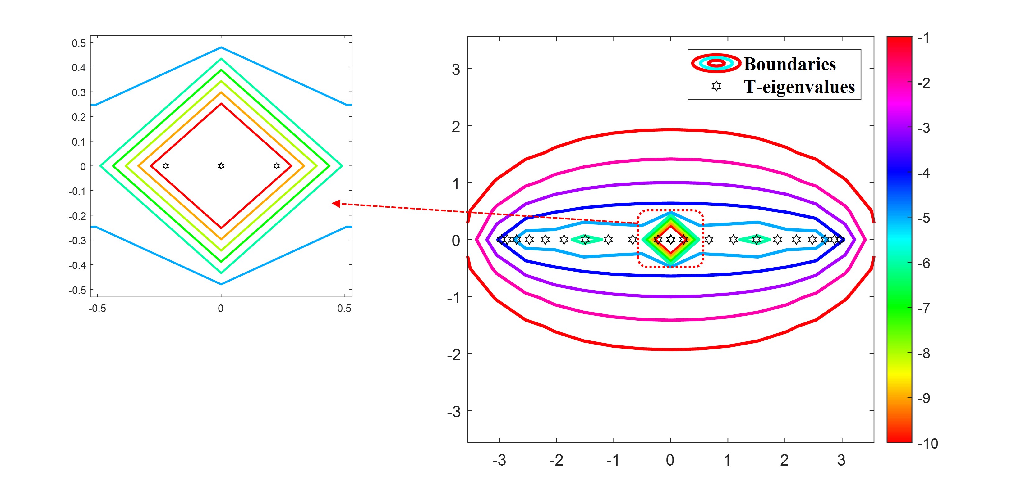
Figure 4: Boundaries of pseudospectra $\Lambda_{\varepsilon}(\mathcal{A})$ for tensor $\mathcal{A}\in\mathbb{R}^{20\times 20\times 3}$ with frontal slices $A_{1}=A_{2}=A_{3}=T_{pz}$ for different $\varepsilon=10^{-1},10^{-2},\ldots,10^{-10}$. The T-eigenvalues are plotted as hexagons.

Example 4.1.

Let $\mathcal{A}$ be a third-order tensor with three frontal faces $A_{1},A_{2}$ and $A_{3}$. First, we consider an example that all frontal faces are the same and each frontal slice is a tridiagonal Toeplitz matrix. That is, $A_{1}=A_{2}=A_{3}=T_{pz}$ with entries given as follows,

$$T_{pz}=\left(\begin{array}[]{ccccc}0&1&&&\\ \frac{1}{4}&0&1&&\\ &\ddots&\ddots&\ddots&\\ &&\frac{1}{4}&0&1\\ &&&\frac{1}{4}&0\end{array}\right)\in\mathbb{R}^{N\times N}.$$

We can see that the size of $\operatorname{bcirc}(\mathcal{A})$ is $3N\times 3N$. However, it is non-symmetrical. Notice that $T_{pz}$ can be symmetrized by a diagonal similarity transformation. That is,

$$DT_{pz}D^{-1}=S,$$

where $D=\operatorname{diag}\left([2,4,\ldots,2^{N}]\right)$ and

$$S=\left(\begin{array}[]{ccccc}0&\frac{1}{2}&&&\\ \frac{1}{2}&0&\frac{1}{2}&&\\ &\ddots&\ddots&\ddots&\\ &&\frac{1}{2}&0&\frac{1}{2}\\ &&&\frac{1}{2}&0\end{array}\right)\in\mathbb{R}^{N\times N}.$$

A tensor $\mathcal{D}\in\mathbb{R}^{N\times N\times 3}$ with frontal faces $D_{1},D_{2}$ and $D_{3}$ is constructed as follows. That is, we let $D_{1}=D$ and choose $D_{2}$ and $D_{3}$ as the zero matrices $O_{N}$. Then another tensor with three frontal faces $D^{-1}$, $O_{N}$, and $O_{N}$ would be the inverse of $\mathcal{D}$. By applying the tensor-tensor multiplication, we get

$$\mathcal{D}*\mathcal{A}*\mathcal{D}^{-1}=\mathcal{S}.$$

It is not hard to calculate that each frontal slice of tensor $\mathcal{S}$ is exactly the symmetric matrix $S$. Then we know that all T-eigenvalues of $\mathcal{A}$ are the same as those T-eigenvalues of $\mathcal{S}$ which are all real and only appear in the real axis since $\operatorname{bcirc}(\mathcal{S})$ is symmetric.

However, the pseudospectra of $\mathcal{A}$ lie a little far from the real axis. We consider a case where $N=20$ and the results are given in Figure 4 in which the T-eigenvalues of tensor $\mathcal{A}$ are plotted as hexagons. The spectral norm is chosen here and we set $\varepsilon=10^{-1},10^{-2},\ldots,10^{-10}$. By the numerical results, we can see that the boundaries of $\Lambda_{\varepsilon}(\mathcal{A})$ may lie far beyond the real axis if $\varepsilon$ is too big.

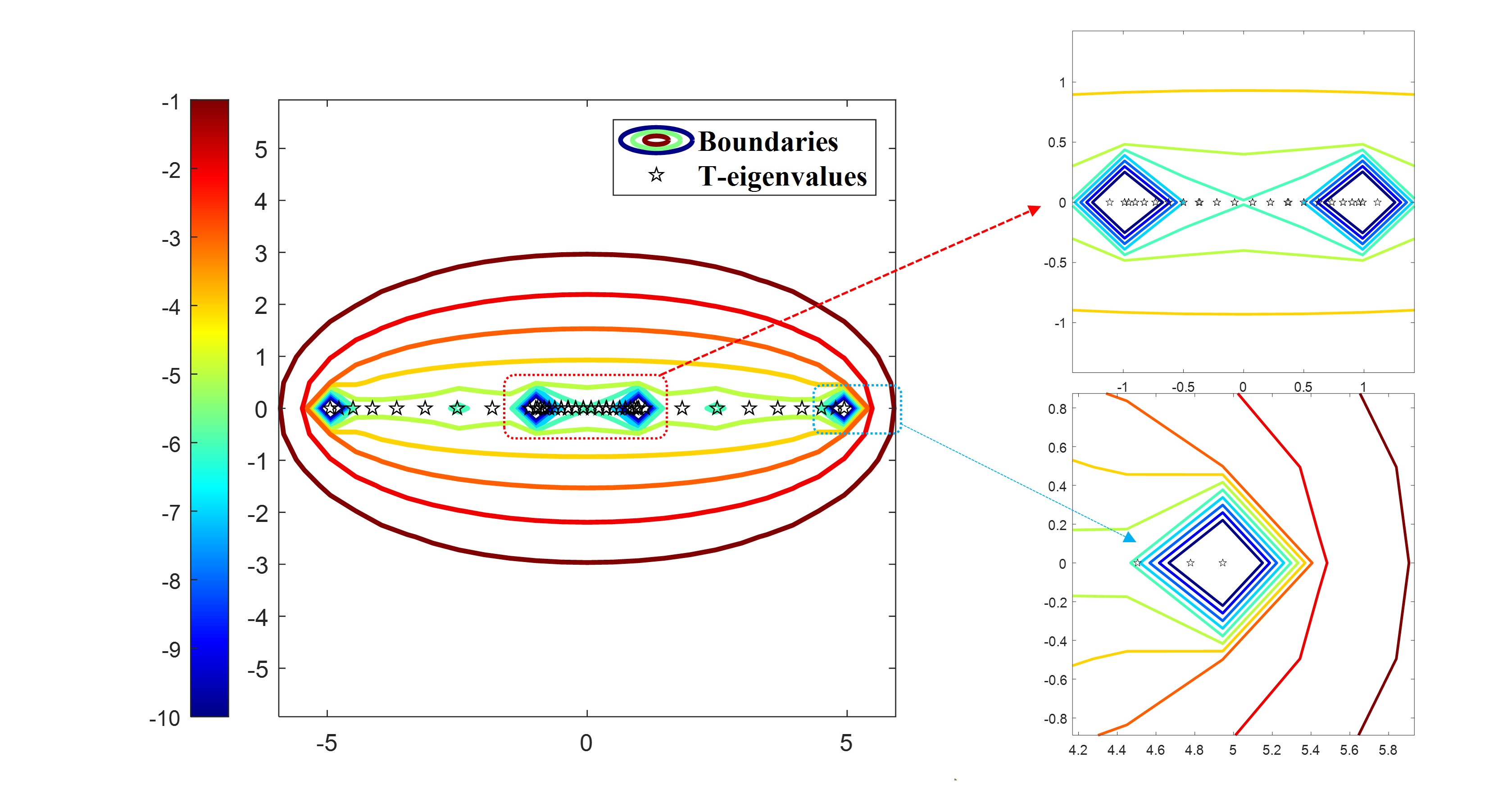
Figure 5: Boundaries of pseudospectra $\Lambda_{\varepsilon}(\mathcal{B})$ for tensor $\mathcal{B}\in\mathbb{R}^{20\times 20\times 3}$ with frontal slices $B_{1}=T_{pz}$ and $B_{2}=B_{3}=2T_{pz}$ for different $\varepsilon=10^{-1},10^{-2},\ldots,10^{-10}$. The T-eigenvalues of tensor $\mathcal{B}$ are plotted as pentagons.

Example 4.2.

Many T-eigenvalues of tensor $\mathcal{A}$ are zero. Another tensor $\mathcal{B}$ with frontal slices satisfying $B_{1}=T_{pz}$ and $B_{2}=B_{3}=2T_{pz}$ is considered next. The corresponding matrix $\operatorname{bcirc}(\mathcal{B})$ is non-symmetrical but all its eigenvalues are real. Similar numerical results on boundaries of pseudospectra $\Lambda_{\varepsilon}(\mathcal{B})$ are given in Figure 5.

Tensors with all real T-eigenvalues are rare generally. In the following, we consider two cases that tensors have complex T-eigenvalues.

Example 4.3.

Suppose $\mathcal{C}\in\mathbb{R}^{20\times 20\times 3}$ is a third-order tensor with frontal slices $C_{1},C_{2}$ and $C_{3}$ such that $C_{3}=2C_{2}=4C_{1}=4T_{pz}$. By 3.1 and using the $\operatorname{bcirc}(\cdot)$ operator, T-eigenvalues which may complex are plotted as crosses ‘$\times$’ in Figure 6. To approximate T-spectra of tensor $\mathcal{C}$, boundaries of $\varepsilon$-pseudospectra with various $\varepsilon$ for tensor $\mathcal{C}$ are also presented in the same figure from which we can find that these boundaries are reasonably tight in locating those real or complex T-eigenvalues.

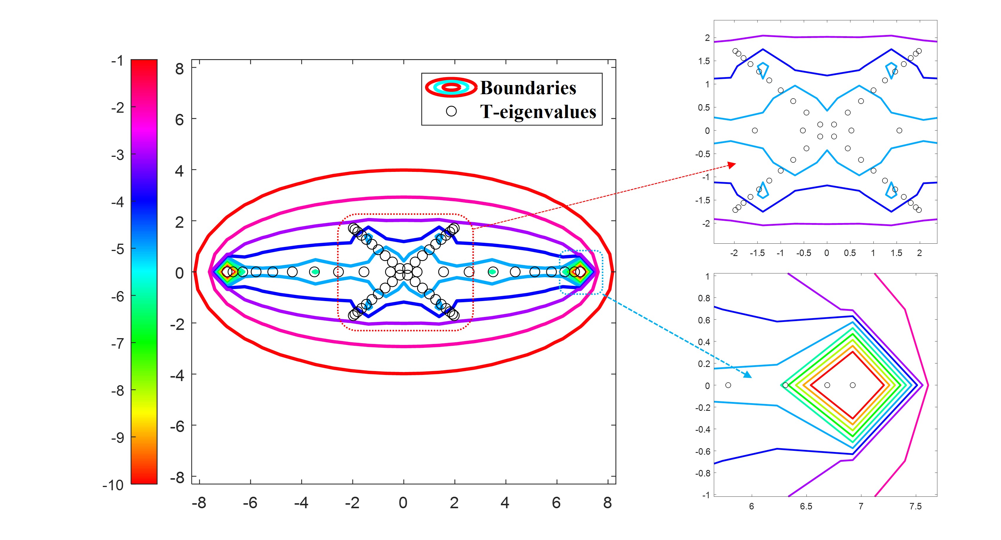
Figure 6: Boundaries of pseudospectra $\Lambda_{\varepsilon}(\mathcal{C})$ for $\varepsilon=10^{-1},10^{-2},\ldots,10^{-10}$ under the condition that $C_{3}=2C_{2}=4C_{1}=4T_{pz}$. The T-eigenvalues of tensor $\mathcal{C}$ are plotted as circles ‘$\circ$’.

Example 4.4.

At last, we consider one more example. Let $F_{1}=T_{pz},F_{2}=10T_{pz}$ and $F_{3}=\operatorname{eye}(N)$. Suppose that they are the three frontal slices of the tensor $\mathcal{F}\in\mathbb{R}^{20\times 20\times 3}$. By a calculation without too much difficulty, one can get all T-eigenvalues of tensor $\mathcal{F}$. They spread along the complex plane with a shape like six-legged starfish; see Figure 7 for an intuitive display. To show the results of $\varepsilon$-pseudospectra, by setting similar parameters in plotting those boundaries, we can also get relatively satisfactory results, just as the results shown in Figure 7.

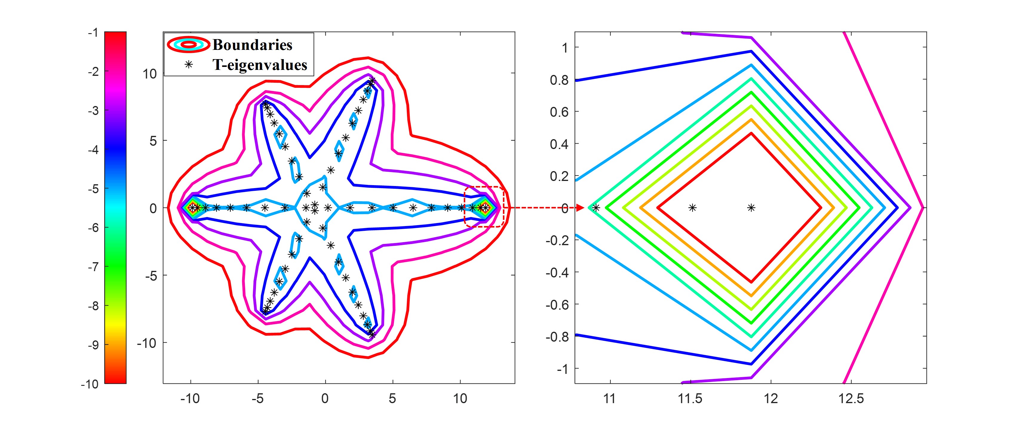
Figure 7: Boundaries of pseudospectra $\Lambda_{\varepsilon}(\mathcal{F})$ for $\varepsilon=10^{-1},10^{-2},\ldots,10^{-10}$ under the condition that $F_{1}=T_{pz},F_{2}=10T_{pz}$ and $F_{3}=\operatorname{eye}(N)$. The T-eigenvalues of tensor $\mathcal{F}$ are plotted by ‘$*$’.

Remark 4.4.

Hundreds of years have witnessed the power of the eigenvalue tool of matrices not only useful in practice but also fundamental in concept [47]. However, in the nonnormal matrix case, eigenvalue analysis may reveal little significance and therefore pseudospectra analysis springs up to remedy such a situation. In the above examples for tensor case, the tensor $\mathcal{A}$ is not normal, that is, $\mathcal{A}*\mathcal{A}^{\mathrm{H}}\neq\mathcal{A}^{\mathrm{H}}*\mathcal{A}$. By an invertible tensor transformation $\mathcal{D}$ under tensor-tensor multiplication sense, we get a normal tensor $\mathcal{S}$ with all real T-eigenvalues. The first two examples show that the pseudospectra of $\mathcal{A}$ lie a little far from the real axis that all T-eigenvalues spread on. This coincides with the results of matrix case greatly [47]. But the last two examples indeed indicate that pseudospectra tool could give a satisfactory capability of approximating all T-eigenvalues, especially for tensor $\mathcal{F}$.

5 Conclusions

This paper investigates perturbation analysis on T-eigenvalues of third-order tensors, building upon the well-known tensor-tensor multiplication. The study extends classical results from matrix perturbation analysis to the third-order case. Notably, we generalize the Gershgorin disc theorem to tensors and demonstrate that all T-eigenvalues are confined within a union of Gershgorin discs. Additionally, we develop three different generalizations of the Bauer-Fike theorem for tensors and explore a generalization of the Kahan theorem into the tensor case. Moreover, we introduce the pseudospectral theory on third tensors, leveraging tensor-tensor multiplication. To characterize tensor $\varepsilon$-pseudospectra, we propose four different definitions and establish their equivalence under the spectral norm case. Several properties of these pseudospectra are presented. To provide visualizations of tensor $\varepsilon$-pseudospectra, various numerical examples are also provided.

In subsequent research, we will delve into the study of rectangular T-eigenvalue problems, i.e., the tensor $\mathcal{A}$ in the expression $\mathcal{A}*\mathcal{X}=\lambda\mathcal{X}$ may have the size of $m\times n\times\ell$, and exploring their properties and computational aspects.

Data availability

No data was used for the research described in the article.

Declaration of Competing Interest

The authors declare that they have no known competing financial interests or personal relationships that could have appeared to influence the work reported in this paper.

References

- [1] F. L. Bauer and C. T. Fike, Norms and exclusion theorems, Numerische Mathematik, 2 (1960), pp. 137–141.
- [2] F. Beik and Y. Saad, On the tubular eigenvalues of third-order tensors, arXiv preprint arXiv:2305.06323, (2023).
- [3] K. Braman, Third-order tensors as linear operators on a space of matrices, Linear Algebra and its Applications, 433 (2010), pp. 1241–1253.
- [4] M. Brazell, N. Li, C. Navasca, and C. Tamon, Solving multilinear systems via tensor inversion, SIAM Journal on Matrix Analysis and Applications, 34 (2013), pp. 542–570.
- [5] Z. Cao and P. Xie, Perturbation analysis for t-product-based tensor inverse, Moore-Penrose inverse and tensor system, Communications on Applied Mathematics and Computation, 4 (2022), pp. 1441–1456.
- [6] Z. Cao and P. Xie, On some tensor inequalities based on the t-product, Linear and Multilinear Algebra, 71 (2023), pp. 377–390.
- [7] S. Y. Chang and Y. Wei, T-product tensors—part II: tail bounds for sums of random T-product tensors, Computational and Applied Mathematics, 41 (2022). Art. 99.
- [8] , T-square tensors—part I: inequalities, Computational and Applied Mathematics, 41 (2022). Art. 62.
- [9] J. Chen, W. Ma, Y. Miao, and Y. Wei, Perturbations of Tensor-Schur decomposition and its applications to multilinear control systems and facial recognitions, Neurocomputing, 547 (2023). Art. 126359.
- [10] K.-W. E. Chu, Generalization of the Bauer-Fike theorem, Numerische Mathematik, 49 (1986), pp. 685–691.
- [11] Y.-N. Cui and H.-F. Ma, The perturbation bound for the T-Drazin inverse of tensor and its application, Filomat, 35 (2021), pp. 1565–1587.
- [12] A. El Hachimi, K. Jbilou, A. Ratnani, and L. Reichel, Spectral computation with third-order tensors using the t-product, Applied Numerical Mathematics. https://doi.org/10.1016/j.apnum.2023.07.011.
- [13] G. H. Golub and C. F. Van Loan, Matrix Computations, The Johns Hopkins University Press, Baltimore, 4th ed., 2013.
- [14] A. Greenbaum, R.-C. Li, and M. L. Overton, First-order perturbation theory for eigenvalues and eigenvectors, SIAM Review, 62 (2020), pp. 463–482.
- [15] F. Han, Y. Miao, Z. Sun, and Y. Wei, T-ADAF: Adaptive data augmentation framework for image classification network based on tensor T-product operator, Neural Processing Letters. https://doi.org/10.1007/s11063-023-11361-7.
- [16] N. Hao, M. E. Kilmer, K. Braman, and R. C. Hoover, Facial recognition using tensor-tensor decompositions, SIAM Journal on Imaging Sciences, 6 (2013), pp. 437–463.
- [17] R. A. Horn and C. R. Johnson, Matrix Analysis, Cambridge University Press, Cambridge, second ed., 2013.
- [18] T. Kato, Perturbation Theory for Linear Operators, Springer-Verlag, Berlin, 1st ed., 1966.
- [19] M. E. Kilmer, K. Braman, and N. Hao, Third-order tensors as operators on matrices: A theoretical and computational framework with applications in imaging, Technical Report 2011-01, Tufts University, 2011.
- [20] M. E. Kilmer, K. Braman, N. Hao, and R. C. Hoover, Third-order tensors as operators on matrices: A theoretical and computational framework with applications in imaging, SIAM Journal on Matrix Analysis and Applications, 34 (2013), pp. 148–172.
- [21] M. E. Kilmer, L. Horesh, H. Avron, and E. Newman, Tensor-tensor algebra for optimal representation and compression of multiway data, Proceedings of the National Academy of Sciences, 118 (2021). Art. e2015851118.
- [22] M. E. Kilmer and C. D. Martin, Factorization strategies for third-order tensors, Linear Algebra and its Applications, 435 (2011), pp. 641–658.
- [23] M. E. Kilmer, C. D. Martin, and L. Perrone, A third-order generalization of the matrix SVD as a product of third-order tensors, Technical Report 2008-4, Tufts University, 2008.
- [24] W.-h. Liu and X.-q. Jin, A study on T-eigenvalues of third-order tensors, Linear Algebra and its Applications, 612 (2021), pp. 357–374.
- [25] Y. Liu, L. Chen, and C. Zhu, Improved robust tensor principal component analysis via low-rank core matrix, IEEE Journal of Selected Topics in Signal Processing, 12 (2018), pp. 1378–1389.
- [26] Y. Liu and H. Ma, Weighted generalized tensor functions based on the tensor-product and their applications, Filomat, 36 (2022), pp. 6403–6426.
- [27] C. Lu, J. Feng, Y. Chen, W. Liu, Z. Lin, and S. Yan, Tensor robust principal component analysis with a new tensor nuclear norm, IEEE transactions on pattern analysis and machine intelligence, 42 (2019), pp. 925–938.
- [28] K. Lund, The tensor t-function: A definition for functions of third-order tensors, Numerical Linear Algebra with Applications, 27 (2020). Art. e2288.
- [29] K. Lund and M. Schweitzer, The fréchet derivative of the tensor t-function, Calcolo, 60 (2023). Art. 35.
- [30] Y.-S. Luo, X.-L. Zhao, T.-X. Jiang, Y. Chang, M. K. Ng, and C. Li, Self-supervised nonlinear transform-based tensor nuclear norm for multi-dimensional image recovery, IEEE Transactions on Image Processing, 31 (2022), pp. 3793–3808.
- [31] Y. Miao, L. Qi, and Y. Wei, Generalized tensor function via the tensor singular value decomposition based on the T-product, Linear Algebra and its Applications, 590 (2020), pp. 258–303.
- [32] , T-Jordan canonical form and T-Drazin inverse based on the T-product, Communications on Applied Mathematics and Computation, 3 (2021), pp. 201–220.
- [33] Y. Miao, T. Wang, and Y. Wei, Stochastic conditioning of tensor functions based on the tensor-tensor product, Pacific Journal of Optimization, 19 (2023), pp. 205–235.
- [34] C. Mo, C. Li, X. Wang, and Y. Wei, Z-eigenvalues based structured tensors: -tensors and strong -tensors, Computational and Applied Mathematics, 38 (2019). Art. 175.
- [35] C. Mo, X. Wang, and Y. Wei, Time-varying generalized tensor eigenanalysis via Zhang neural networks, Neurocomputing, 407 (2020), pp. 465–479.
- [36] E. Newman and M. E. Kilmer, Nonnegative tensor patch dictionary approaches for image compression and deblurring applications, SIAM Journal on Imaging Sciences, 13 (2020), pp. 1084–1112.
- [37] M. Pakmanesh and H. Afshin, M-numerical ranges of odd-order tensors based on operators, Annals of Functional Analysis, 13 (2022), pp. 1–22.
- [38] L. Qi, Eigenvalues of a real supersymmetric tensor, Journal of Symbolic Computation, 40 (2005), pp. 1302–1324.
- [39] L. Qi and X. Zhang, T-quadratic forms and spectral analysis of T-symmetric tensors, arXiv preprint arXiv:2101.10820, (2021).
- [40] L. Rayleigh, The Theory of Sound. Volume I, Macmillan, London, 1927.
- [41] F. Rellich, Perturbation Theory of Eigenvalue Problems, Gordon and Breach Science, New York, London, Paris, 1969.
- [42] E. Schrödinger, Quantisierung als Eigenwertproblem, Annalen Phys., 386 (1926), pp. 109–139.
- [43] X. Shi and Y. Wei, A sharp version of Bauer–Fike’s theorem, Journal of Computational and Applied Mathematics, 236 (2012), pp. 3218–3227.
- [44] G. W. Stewart and J. Sun, Matrix Perturbation Theory, Academic Press, Boston, 1990.
- [45] J. Sun, Matrix Perturbation Analysis (In Chinese), Academic Press, Beijing, 1987.
- [46] L. Tang, Y. Yu, Y. Zhang, and H. Li, Sketch-and-project methods for tensor linear systems, Numerical Linear Algebra with Applications, 30 (2023). Art. e2470.
- [47] L. N. Trefethen and M. Embree, Spectra and Pseudospectra: The Behavior of Nonnormal Matrices and Operators, Princeton University Press, Princeton, 2005.
- [48] E. Turatti, On tensors that are determined by their singular tuples, SIAM Journal on Applied Algebra and Geometry, 6 (2022), pp. 319–338.
- [49] X. Wang, M. Che, C. Mo, and Y. Wei, Solving the system of nonsingular tensor equations via randomized Kaczmarz-like method, Journal of Computational and Applied Mathematics, 421 (2023). Art. 114856.
- [50] X. Wang, P. Wei, and Y. Wei, A fixed point iterative method for third-order tensor linear complementarity problems, Journal of Optimization Theory and Applications, 197 (2023), pp. 334–357.
- [51] Y. Wang and Y. Yang, Hot-SVD: higher order t-singular value decomposition for tensors based on tensor–tensor product, Computational and Applied Mathematics, 41 (2022). Art. 394.
- [52] P. Wei, X. Wang, and Y. Wei, Neural network models for time-varying tensor complementarity problems, Neurocomputing, 523 (2023), pp. 18–32.
- [53] T. Wu, Graph regularized low-rank representation for submodule clustering, Pattern Recognition, 100 (2020). Art. 107145.
- [54] Y. Yang and J. Zhang, Perron-Frobenius type theorem for nonnegative tubal matrices in the sense of t-product, Journal of Mathematical Analysis and Applications, 528 (2023). Art. 127541.
- [55] X.-L. Zhao, W.-H. Xu, T.-X. Jiang, Y. Wang, and M. K. Ng, Deep plug-and-play prior for low-rank tensor completion, Neurocomputing, 400 (2020), pp. 137–149.
- [56] M.-M. Zheng, Z.-H. Huang, and Y. Wang, T-positive semidefiniteness of third-order symmetric tensors and t-semidefinite programming, Computational Optimization and Applications, 78 (2021), pp. 239–272.