Observer-based Control for Vehicle Platooning
with a Leader of Varying Speed

Abstract

This paper studies the internal stability and string stability of a vehicle platooning of constant time headway spacing policy with a varying-speed leader using a multiple-predecessor-following strategy via vehicle-to-vehicle communication. Unlike the common case in which the leader’s speed is constant and different kinds of Proportional-Integral-Derivative controllers are implemented, in this case, the fact that the leader has a time-varying speed necessitates the design of an observer. First, in order to estimate its position, speed and acceleration error with respect to the leader, each follower designs an observer. The observer is designed by means of constructing an observer matrix whose parameters should be determined. We simplifies the design of the matrix of the observer in such a way that the design boils down to choosing a scalar value. The resulting observer turns out to have a third order integrator dynamics, which provides an advantage of simplifying the controller structure and, hence, derive conditions for string stability using a frequency response method. A new heuristic searching algorithm is developed to deduce the controller parameter conditions, given a fixed time headway, for string stability. Additionally, a bisection-like algorithm is incorporated into the above algorithm to obtain the minimum (with some deviation tolerance) available value of the time headway by fixing one controller parameter. The effectiveness of the internal and string stabilities of the proposed observer-based controller is demonstrated via comparison examples.

I Introduction

Platoon systems in transportation networks designate a class of network systems where automated vehicles, typically arranged in a string, cooperate via some distributed control protocol, or coupling, in order to travel along the longitudinal direction [1]. Vehicle platooning can lead to an increase in road throughput and travel safety, while reducing travel time, fuel consumption and CO₂ emission due to the reduced air drag. Typically, the designed distributed control protocol needs to guarantee internal stability and string stability of the platoon system, e.g., see [2, 3, 4, 5]. The internal stability characterizes the platoon stability as a system, which translates to having a vehicle match its speed to the speed of the vehicle in front of it, or the platoon leader, while keeping a desired inter-vehicle distance [6]. The string stability enable vehicle platoons to be able to attenuate the error signals when propagating down the vehicle string [7]. Specifically, if the system is string stable, then: (i) vehicles can attain and keep the desired configuration; (ii) the effects of disturbances are attenuated along the string [8].

It is known that string stability is dramatically influenced by the spacing policy which is one of the main components of a platoon that determines the desired inter-vehicle distance. There are two main spacing policies: constant distance spacing policy (CDS) and constant time headway spacing (CTHS) policy. While a platoon can be string unstable under CDS policy with the predecessor-following (PF) information flow topology (IFT) [3] or the bidirectional (BD) IFT [9], it is string stable with the leader-predecessor-following (LPF) IFT with the aid of vehicle-to-vehicle (V2V) communication technologies. However, in the LPF topology, each follower needs to know the leader’s information via communication channels, which is a big barrier when the platoon size becomes larger and larger. On the contrary, the CTHS policy in which each vehicle regulates its desired distance from its predecessor by utilizing a linear function of speed (leader/predecessor speed or its own speed) with a constant time headway as the proportional gain, can lead the platoon system to be string stable with PF topology [10]. As PF topology is more practical in reality, introducing time headway may compromise the transport throughput, since the inter-vehicle distance increases as the speed grows. It is therefore desirable to reduce time headway while guaranteeing string stability [11]. Following this trail of thought, authors in [5] utilize the CTHS policy with multiple-predecessor-following (MPF) topology by designing a Proportional-Integral-Derivative (PID) controller to derive the lower bound of the time headway which is related to the number of multiple predecessor. This spacing policy strategy and communication topology is also adopted in this paper. For a more detailed literature review about the above policies and topologies, please refer to [5].

For the vehicle platooning, one key issue is to guarantee string stability. Historically, the work on string stability can be traced back to [12] and to the California PATH program [13]. There are mainly three analysis methods being used to derive sufficient conditions for proving string stability; namely, $z$-domain, $s$-domain and time-domain analysis methods. For a thorough discussion about the relations and comparisons of the above three methods, survey paper [14] is recommended. Basically, for general nonlinear systems, the time-domain method is usually adopted by using the techniques of Lyapunov functions and eigenvalue analysis; e.g., see [15, 8]. For linear systems, the $s$-domain methods which construct transfer functions between the outputs and inputs of systems by Laplace transform and determine whether the $\mathcal{H}_{\infty}$ norm of the transfer function is smaller or equal to one, are commonly used; see, e.g., [10, 5, 16, 17, 18]. Since the commonly used third integrator platoon dynamics is investigated in this paper, the $s$-domain method is adopted here.

In the literature, all works related to vehicle platooning except a few ones consider the leader with a constant speed. It is worth noting that investigating the case in which the leading vehicle is of varying speed with specific dynamics is very meaningful as it is the case of how a real vehicle moves. Authors in [8] designed a control protocol allowing to track a desired (possibly, non-constant) reference speed, i.e., the leader does not have a specific dynamics and is regarded as a state to be communicated to the followers directly. In [19], authors proposed a truck-platoon model in which the speed of the virtual truck is required to be known to all vehicles (including the leader) of the platoon. The advantage is that this speed can change over time, but it is the global information which can limit the platoon application when the number of vehicles is large. This paper focuses on those platoons, which have leaders of varying speed and we have proposed an observer-based controller that can guarantee the internal stability and string stability, while no global information is needed (i.e., only a limited number of followers are connected to the leading vehicle). Specifically, the distributed observer is proposed for estimating the position, speed and acceleration error between each vehicle and the leader; then, this observer is used to construct the controller for each follower vehicle. This is one contribution of this paper.

Considering the leader with a constant speed, i.e., zero acceleration, delivers the advantage that it is enough to design PID controllers with simpler $\mathcal{H}_{\infty}$ norm functions. While dealing with the platoon, whose leader has a nonzero acceleration leads to a much more complicated $\mathcal{H}_{\infty}$ norm of the string stability transfer function. In this paper, we have proposed a new calculation technique for analyzing this $\mathcal{H}_{\infty}$ norm to deduce conditions for the string stability property. This is another contribution of this work.

The objective of this paper is the following: designing a platoon system under the directed MPF IFT in which the leader of specific dynamics (see Eq. (2)) has a time-varying speed. On the way to achieve this objective, we made the following contributions.

• First, a distributed observer for estimating the position, speed and acceleration error between each vehicle and the leader is proposed.

• Then, a controller is designed based on the proposed observer. This observer-based controller is fully distributed, i.e., no global information is required. As a consequence, unlike other works in the literature [15, 20, 8, 21] where all followers need the leader vehicle’s information, the controller in this paper can be applied to large-scale platoon systems.

• The parameters of the observer and the controller are designed such that the internal and string stability of the platoon system are guaranteed. As the $\mathcal{H}_{\infty}$ norm of the string stability transfer function becomes more complicated because of this observer-based controller rather than the commonly used PID controller, a new calculation mechanism is proposed, i.e., a heuristic searching algorithm, in order to determine the range of those parameters, given a fixed time headway. This mechanism can also be applied to analyze the string stability via the $\mathcal{H}_{\infty}$ norm of PID controller based transfer functions.

• In addition, a bisection-like algorithm is incorporated into the above algorithm to obtain the minimum (within a tolerance) available value of the time headway.

To the best of the authors’ knowledge, this is the first effort towards controlling platoons under the directed MPF topology while having a leader of varying speed without any global information, such as eigenvalues of the communication graph (e.g., in [22]) or without a requirement that all followers need to know the (virtual) leader’s information (e.g., in [19]). The authors have introduced a preliminary version [23] in which only the numeric method by trials and errors is used to design controller parameters while a theoretical algorithm based on a new calculation mechanism is proposed here to design controller parameters to guarantee the string stability.

The rest of this paper is organized as follows. Section II gives some notations and mathematical preliminaries. Section III presents the vehicle model, the spacing policy and the control objective. In Section IV, a distributed observer is proposed with the internal stability and string stability presented. Some corroborating simulations are provided in Section V. Finally, in Section VI we conclude the paper and discuss future directions.

II Notation

$\mathbb{R}^{m\times n}$ and $\mathbb{R}^{n}$ are respectively the $m\times n$ real matrix space and $n$-dimensional Euclidean vector space. For the square matrix $A$, $\mathrm{Re}(\lambda(A))$ represents the real part of eigenvalues of $A$. For any integers $a$ and $b$, with $a\leq b$, denote $\textbf{I}_{a}^{b}=\{a,a+1,\ldots,b\}$. The $\mathcal{H}_{\infty}$ norm of a stable scalar transfer function $H(s)$ is denoted by $\left\|H\right\|_{\infty}\triangleq\sup_{\omega\in\mathbb{R}}|H(j\omega)|$.

In a weighted graph $\mathcal{G}=(\mathcal{N,E,A})$, $\mathcal{N}=\left\{1,2,\ldots,N\right\}$ and $\mathcal{E}\subseteq\mathcal{N\times N}$ are the nodes and edges, respectively. $\mathcal{A}=\left[a_{ij}\right]\in\mathbb{R}^{N\times N}$ is the weighted adjacency matrix, where $a_{ij}=1,\left(i,j\right)\in\mathcal{E}$ and $a_{ij}=0$ otherwise. An edge $\left(j,i\right)\in\mathcal{E}$ means agent $j$ can get information from agent $i$. A directed path from node $i$ to $j$ is a sequence of nodes $i=l_{1},l_{2},\ldots,l_{t}=j$ such that link $(l_{m+1},l_{m})\in\mathcal{E}$ for all $m=1,2,\ldots,t-1$. The Laplacian matrix $\mathcal{L}=\left[l_{ij}\right]\in\mathbb{R}^{N\times N}$ is defined as $l_{ij}=-a_{ij},i\neq j$ and $l_{ii}=\sum_{j\neq i}a_{ij}$. All nodes that can transmit information to node $v_{i}$ directly are said to be in-neighbors of node $v_{i}$ and belong to the set $\mathcal{N}^{-}_{i}=\{v_{j}\in\mathcal{V}\;|\;\varepsilon_{ij}\in\mathcal{E}\}$. The nodes that receive information from node $v_{i}$ belong to the set of out-neighbors of node $v_{i}$, denoted by $\mathcal{N}^{+}_{i}=\{v_{l}\in\mathcal{V}\;|\;\varepsilon_{li}\in\mathcal{E}\}$. All in-neighbors and out-neighbors of node $v_{i}$ combined are regarded the neighbors of node $v_{i}$.

III Problem formulation

III-A Longitudinal vehicle platooning dynamics

The vehicle string is made up of $N$ follower vehicles with a leader vehicle labeled $0$. In the longitudinal dynamics, usually it is assumed that the input of the vehicle is the throttle system while the output is the position. Thus, the following model is used to describe the relation between the desired acceleration to the throttle system and the position of the follower vehicle [16, 2, 24]:

$$\dot{x}_{i}(t)=\underbrace{\begin{bmatrix}0&1&0\\ 0&0&1\\ 0&0&-\frac{1}{\tau}\end{bmatrix}}_{\eqqcolon A}x_{i}(t)+\underbrace{\begin{bmatrix}0\\ 0\\ \frac{1}{\tau}\end{bmatrix}}_{\eqqcolon B}u_{i}(t),i\in\textbf{I}_{1}^{N},$$ (1)

where $x_{i}(t)\coloneqq[p_{i}(t),v_{i}(t),a_{i}(t)]^{T},p_{i}(t),v_{i}(t),a_{i}(t)$ represent the longitudinal position, speed, and acceleration of vehicle $i,i\in\textbf{I}_{1}^{N}$, respectively; $\tau$ is the engine time constant and $u_{i}(t)$ is the vehicle input to be designed; $A\in\mathbb{R}^{3\times 3},B\in\mathbb{R}^{3\times 1}$. One can verify that $(A,B)$ is controllable.

The leader vehicle dynamics we investigate here is

$$\dot{p}_{0}(t)=v_{0}(t),\,\dot{v}_{0}(t)=a_{0}(t),\,\dot{a}_{0}(t)=-\frac{1}{\tau}a_{0}(t),$$ (2)

which is also

$$\dot{x}_{0}(t)=Ax_{0}(t).$$ (3)

Note that many works, e.g., [25, 5, 26, 27], assume that $v_{0}(t)$ is a constant, i.e., $a_{0}(t)=0,u_{0}(t)=0$, which is quite restrictive. In this work, we assume that leader’s speed can be time-varying, though without any control input, i.e., $u_{0}(t)=0$. For the case where the leader’s speed is constant, the commonly used PID controller is enough to guarantee that the platooning system is stable theoretically, e.g., see [25, 5]. However, when the leader’s dynamics changes to (3), the stability cannot be easily guaranteed theoretically by PID controllers.

III-B Inter-vehicle distance using constant time headway

The desired inter-vehicle distance between vehicle $i$ and vehicle $i-j$ is given by (e.g., in [5]):

$$d_{i,i-j}(t)=\sum_{k=i}^{i-j+1}h_{k}v_{k-1}(t)+jD,$$ (4)

where $h_{k}$ is the time headway of vehicle $k$ and $D$ is the standstill desired gap between vehicle $i$ and $i-1$ (we assume the gap between any two consecutive vehicles are the same since the platoon is homogeneous, to simplify the calculations). Moreover, since the platooning of homogeneous vehicles is investigated here, we can set $h_{k}=h,\forall k\in\textbf{I}_{1}^{N}$ for convenience. One can see the adopted CTHS policy in this paper is a linear function of predecessor speed with a constant time headway as the proportional gain.

III-C Inter-vehicle communication structure

Assumption 1

The connected vehicles in the platoon are interconnected via the MPF IFT with the leader vehicle as the root node, and the number of predecessors that follower vehicle $i$ has is $r_{i},1\leq r_{i}\leq i,i\in\textbf{I}_{1}^{N}$.

Under Assumption 1, The adjacency matrix $\mathcal{A}=[a_{ij}]\in\mathbb{R}^{(N+1)\times(N+1)}$ of MPF IFT has the property of $a_{0j}=0,a_{ij}=0,\forall i<j,i\in\textbf{I}_{1}^{N},j\in\textbf{I}_{1}^{N}$, i.e., $\mathcal{A}$ becomes a lower-triangular matrix. As a result, the Laplacian matrix $\mathcal{L}$ has the same property. Partition $\mathcal{L}$ as $\mathcal{L}=\begin{bmatrix}0&0_{1\times N}\\ \mathcal{L}_{N\times 1}&\mathcal{L}_{1}\end{bmatrix},$ where $\mathcal{L}_{1}\in\mathbb{R}^{N\times N}$ with $l_{ii}=r_{i},i\in\textbf{I}_{1}^{N}$.

III-D Control objectives

Define the desired position for the $i$th vehicle related to its predecessor vehicle as

$$\bar{p}_{i}^{d}(t)=p_{i-1}(t)-d_{i,i-1}(t),$$ (5)

where $d_{i,i-1}(t)=hv_{i-1}(t)+D$ can be calculated from (4). Then, define the predecessor-follower position, speed and acceleration errors for the $i$th vehicle related to its predecessor vehicle as follows:

$$\bar{p}_{i}(t)= p_{i}(t)-\bar{p}_{i}^{d}(t)=p_{i}(t)-p_{i-1}(t)+hv_{i-1}(t)+D,$$

$$\bar{v}_{i}(t)= v_{i}(t)-v_{i-1}(t),$$

$$\bar{a}_{i}(t)= a_{i}(t)-a_{i-1}(t),i\in\textbf{I}_{1}^{N}.$$ (6)

Denote an augmented variable $\bar{x}_{i}(t)\coloneqq[\bar{p}_{i}(t),\bar{v}_{i}(t),\bar{a}_{i}(t)]^{T}$ and under Assumption 1, the platooning is required to track a varying-speed leader, where the following objectives are set:

• convergence of the predecessor-follower platooning tracking error $\bar{x}_{i}(t)$;

• guarantee of the predecessor-follower string stability.

IV Main results

For the convenience of presentation, the time index $(t)$ is omitted in this section. In order to achieve the previous objectives, we first provide a leader-following platooning tracking error model which is related to the leader; then, a distributed observer is proposed to estimate this error; thereafter, the link between this error with the predecessor-follower platooning tracking error $\bar{x}_{i}$ is presented and the convergence is proved to achieve objective $\mathrm{O_{1}}$; finally, the predecessor-follower string stability is demonstrated, thus achieving objective $\mathrm{O_{2}}$.

IV-A Leader-following platooning tracking error model

Define the desired position for the $i-$th follower vehicle from the leader vehicle as

$$p_{i}^{d}=p_{0}-\left(\sum_{k=1}^{i}h_{k}v_{0}+iD\right)=p_{0}-{i}\left(hv_{0}+D\right).$$

Then, the leader-following position, speed and acceleration errors are respectively defined as follows:

$$\tilde{p}_{i}= p_{i}-p_{i}^{d}=p_{i}-p_{0}+{i}(hv_{0}+D),$$

$$\tilde{v}_{i}= v_{i}-v_{0},$$

$$\tilde{a}_{i}= a_{i}-a_{0}.$$ (7)

Now, we calculate $\dot{\tilde{p}}_{i}$ first as

$$\dot{\tilde{p}}_{i}=\tilde{v}_{i}+iha_{0}.$$ (8)

By defining the augmented variable $\tilde{x}_{i}$ as $\tilde{x}_{i}\coloneqq[\tilde{p}_{i},\tilde{v}_{i},\tilde{a}_{i}]^{T},$ from (1) we obtain

$$\dot{\tilde{x}}_{i}=A\tilde{x}_{i}+Bu_{i}+B_{1}\Omega_{i},i\in\textbf{I}_{1}^{N},$$ (9)

where $B_{1}=\begin{bmatrix}1&0&0\end{bmatrix}^{T},\Omega_{i}=iha_{0}$. Also, from (2) we have that $\dot{a}_{0}=-\frac{1}{\tau}a_{0}\Rightarrow\lim_{t\rightarrow\infty}a_{0}(t)=0$. As a result, we deduce that $\lim_{t\rightarrow\infty}\Omega_{i}(t)=0$.

IV-B Distributed observer design

Analyzing the construction of the predecessor-follower platooning tracking error $\bar{x}_{i}$ in (6) and the leader-following platooning tracking error $\tilde{x}_{i}$ in (7), we find out that as $\tilde{x}_{i}\to 0$, then eventually $v_{i}=v_{j}=v_{0}$ and $a_{i}=a_{j}=a_{0}$. As a result, $\bar{v}_{i}=0$, $\bar{a}_{i}=0$ and $\tilde{x}_{i}\rightarrow 0\Rightarrow\tilde{p}_{i}=0,\tilde{p}_{j}=0\Rightarrow\tilde{p}_{i}-\tilde{p}_{i-1}=p_{i}-p_{i-1}+hv_{0}+D=0\Rightarrow\bar{p}_{i}=0$, i.e., $\tilde{x}_{i}\rightarrow 0\Rightarrow\bar{x}_{i}\rightarrow 0$. Therefore, objective $\mathrm{O_{1}}$ can be transformed to prove the convergence of $\tilde{x}_{i}$. In fact, the relation between $\bar{x}_{i}$ and $\tilde{x}_{i}$ is

$$\bar{x}_{1}=\tilde{x}_{1},\,\bar{x}_{i}=\tilde{x}_{i}-\tilde{x}_{i-1}+\begin{bmatrix}h\tilde{v}_{i-1}&0&0\end{bmatrix}^{T},i\in\textbf{I}_{2}^{N}.$$ (10)

The idea is to design a distributed observer as $\hat{x}_{i}\coloneqq[\hat{p}_{i},\hat{v}_{i},\hat{a}_{i}]^{T}\in\mathbb{R}^{3}$ with $\hat{x}_{i}(0)=0$ to estimate the leader-following platooning error $\tilde{x}_{i}$. From Assumption 1, the neighbor of vehicle $1$ is only the leader, which means vehicle $1$ can receive the information of $p_{0},v_{0},a_{0}$. As a consequence, the observer mathematical format is divided into $\hat{x}_{1}$ and $\hat{x}_{i},i\in\textbf{I}_{2}^{N}$, respectively, as follows:

$$\dot{\hat{x}}_{1}= A\hat{x}_{1}+Bu_{1}+BK(\bar{x}_{1}-\hat{x}_{1})+BLa_{10}(\bar{x}_{1}-\hat{x}_{1}),$$

$$\dot{\hat{x}}_{i}= A\hat{x}_{i}+Bu_{i}+BK(\bar{x}_{i}-\hat{x}_{i})$$

$$+BL\{\sum_{j=1}^{i-1}a_{ij}[\begin{bmatrix}p_{i}-p_{j}+\sum_{k=j+1}^{i}hv_{j}+(i-j)D\\ v_{i}-v_{j}\\ a_{i}-a_{j}\end{bmatrix}-(\hat{x}_{i}-\hat{x}_{j})]+a_{i0}(\bar{x}_{i}-\hat{x}_{i})\},i\in\textbf{I}_{2}^{N},$$ (11)

where $\bar{x}_{i},i\in\textbf{I}_{1}^{N}$ is defined in (6) and $a_{ij}$ is the element of the adjacency matrix $\mathcal{A}$ with $a_{i0}=1,i\in\textbf{I}_{1}^{r}$ and $a_{i0}=0,i\in\textbf{I}_{r+1}^{N}$; observer parameters $L\in\mathbb{R}^{1\times 3}$ and $K\in\mathbb{R}^{1\times 3}$ will be designed later. One can see that the observer of vehicle $i$ requires the relative position, the relative velocity, the relative acceleration with respect to its neighbors, and additionally the velocity $v_{j}$ and observer information $\hat{x}_{j}$ from all its neighbors $v_{j}\in\mathcal{N}_{i}$. To avoid the excessive communication, a special design of the parameter matrix $L$ will be presented in Sec. IV-C, in which the information needed will be much less, as it will be demonstrated in Sec. IV-D. Note that $a_{i0}=0,i\in\textbf{I}_{r+1}^{N}$ means vehicles $r+1,r+2,\ldots,N$ do not need to know the leader vehicle’s information, which is a crucial departure from the controller in [19] in which the velocity of the virtual truck should be known to all vehicles in the platoon. Actually, we use the information of predecessors (e.g., $\bar{x}_{i}$) to design observer to estimate $\tilde{x}_{i}$ which implicitly includes the leader vehicle’s information.

Denote the observer estimating error $\xi_{i}\in\mathbb{R}^{3}$ as

$$\xi_{i}\coloneqq\tilde{x}_{i}-\hat{x}_{i},i\in\textbf{I}_{1}^{N}.$$ (12)

Remark 1

Recall that the purpose of designing the observer is to have $\lim_{t\rightarrow\infty}\xi_{i}(t)=0$. From definitions of $\bar{x}_{i}$ in (6) and $\tilde{x}_{i}$ in (7), one can see $\bar{x}_{1}=\tilde{x}_{1}$; then, one can design $\hat{x}_{1}=\tilde{x}_{1}$ directly to have $\xi_{1}=0$ for all time. However, with this design, we cannot guarantee the platoon string stability theoretically as we will demonstrate in Section IV-D.

After some algebraic manipulations, we obtain that

$$p_{i}-p_{j}+\sum_{k=j+1}^{i}hv_{j}+(i-j)D =p_{i}-p_{0}+ihv_{0}-[p_{j}-p_{0}+jhv_{0}+(i-j)hv_{0}]+(i-j)hv_{j}+(i-j)D$$

$$=\tilde{p}_{i}-\tilde{p}_{j}+(i-j)h\tilde{v}_{j}.$$

Hence, the proposed observer for $\hat{x}_{i}$, $i\in\textbf{I}_{1}^{N}$ in (11) changes to

$$\dot{\hat{x}}_{1}=A\hat{x}_{1}+Bu_{1}+BK\xi_{1}+BL\xi_{1},$$

$$\dot{\hat{x}}_{i}=A\hat{x}_{i}+Bu_{i}+BK\xi_{i}+BL\sum_{j=1}^{i}l_{ij}\xi_{j}+\underbrace{BL\sum_{j=1}^{i-1}a_{ij}\begin{bmatrix}(i-j)h\tilde{v}_{j}\\ 0\\ 0\end{bmatrix}-B(a_{i0}L+K)\begin{bmatrix}\tilde{p}_{i-1}-h\tilde{v}_{i-1}\\ \tilde{v}_{i-1}\\ \tilde{a}_{i-1}\end{bmatrix}}_{\eqqcolon\Pi_{i-1}}.$$ (13)

Now, based on the leader-following platooning error dynamics $\tilde{x}_{i}$ in (9), we design the control input as

$$u_{i}=-K\hat{x}_{i},i\in\textbf{I}_{1}^{N},$$ (14)

such that

$$\dot{\tilde{x}}_{i}=(A-BK)\tilde{x}_{i}+BK\xi_{i}+B_{1}\Omega_{i}.$$ (15)

Due to the fact that $\lim_{t\rightarrow\infty}\Omega_{i}(t)=0$ in (8), if $\lim_{t\rightarrow\infty}\xi_{i}(t)=0$ and we design $K$ such that $A-BK$ is Hurwitz, then, $\lim_{t\rightarrow\infty}\tilde{x}_{i}(t)=0$.

Theorem 1

Under Assumption 1, the predecessor-follower platooning tracking error will converge to zero asymptotically, i.e., $\lim_{t\rightarrow\infty}\bar{x}_{i}(t)=0$, by designing parameter matrices $K$ and $L$ such that $A-BK$, $A-BK-l_{ii}BL$ are Hurwitz, where $l_{ii}$ is the diagonal element of the matrix $\mathcal{L}_{1}$.

Proof:

First, we begin with the platooning convergence of vehicle $1$. Based on Eqs. (12)-(15), the observer error dynamics becomes

$$\dot{\xi}_{1}=(A-BK-BL)\xi_{1}+B_{1}\Omega_{1}.$$ (16)

It is easy to have $\lim_{t\rightarrow\infty}\xi_{1}(t)=0$ based on the condition that $(A-BK-BL)$ is Hurwitz ($l_{ii}=1$ as the leader is the only neighbor of vehicle $1$ in the platooning) and $\lim_{t\rightarrow\infty}\Omega_{1}(t)=0$. Again from (15), based on $\lim_{t\rightarrow\infty}\xi_{1}(t)=0$, $\lim_{t\rightarrow\infty}\tilde{x}_{1}(t)=0$ can be proved based on $A-BK$ is Hurwitz. Since $\bar{x}_{1}=\tilde{x}_{1}$, we have $\lim_{t\rightarrow\infty}\bar{x}_{1}(t)=0$.

Then, for vehicle $2$, similar to the previous calculation, we have

$$\dot{\xi}_{2}= (A-BK)\xi_{2}+B_{1}\Omega_{2}-BL\sum_{j=1}^{2}l_{2j}\xi_{j}-\Pi_{1}$$ (17)

$$= (A-BK-l_{22}BL)\xi_{2}+B_{1}\Omega_{2}-BLl_{21}\xi_{1}-\Pi_{1}.$$

From (13), one can see $\Pi_{1}$ consists of $\tilde{p}_{1},\tilde{v}_{1},\tilde{a}_{1}$ which already all converge to zero because of $\lim_{t\rightarrow\infty}\tilde{x}_{1}(t)=0$ for vehicle $1$. In addition, based on $\lim_{t\rightarrow\infty}\xi_{1}(t)=0$ and $\lim_{t\rightarrow\infty}\Omega_{2}(t)=0$, we get $\lim_{t\rightarrow\infty}\xi_{2}(t)=0$. Furthermore, $\lim_{t\rightarrow\infty}\tilde{x}_{2}(t)=0$ from (15). What is more, based on $\lim_{t\rightarrow\infty}v_{1}(t)=v_{0}$ from $\lim_{t\rightarrow\infty}\tilde{x}_{1}(t)=0$ for vehicle $1$, we can have $\lim_{t\rightarrow\infty}\bar{x}_{2}(t)=\lim_{t\rightarrow\infty}(\tilde{x}_{2}(t)-\tilde{x}_{1}(t))=0$.

Finally, for vehicle $i,i=3,4,\ldots,N$, we can get

$$\dot{\xi}_{i}=(A-BK-l_{ii}BL)\xi_{i}+B_{1}\Omega_{i}-BL\sum_{j=1}^{i-1}l_{ij}\xi_{j}-\Pi_{i-1}.$$ (18)

From the MPF topology in Assumption 1, $a_{ij}=1,l_{ij}=-1,j\in\textbf{I}_{i-r_{i}}^{i-1}$ and $a_{ij}=0,l_{ij}=0,j\in\textbf{I}_{i-r_{i}-1}^{1}$. In reality, $\Pi_{i-1}$ in (13) consists of $\tilde{p}_{i-1},\tilde{v}_{i-1},\tilde{a}_{i-1}$ and $\tilde{v}_{i-2},\ldots,\tilde{v}_{i-r_{i}}$. From Eqs. (16) and (17), one can see for current vehicle $i$, both $\xi_{j}$ and $\tilde{x}_{j}$ of its preceding vehicle $j$ converge to zero asymptotically, i.e., $\lim_{t\rightarrow\infty}\Pi_{i-1}(t)=0$. Thus, it is easy to have $\lim_{t\rightarrow\infty}\xi_{i}(t)=0\Rightarrow\lim_{t\rightarrow\infty}\tilde{x}_{i}(t)=0,i\in\textbf{I}_{3}^{N}$. Similarly, $\lim_{t\rightarrow\infty}\bar{x}_{i}(t)=\lim_{t\rightarrow\infty}(\tilde{x}_{i}(t)-\tilde{x}_{i-1}(t))=0,i\in\textbf{I}_{3}^{N}$ based on $\lim_{t\rightarrow\infty}v_{i-1}(t)=v_{0}$ for vehicle $i-1$. ∎

Remark 2

The proof of Theorem 1 states that the platooning tracking error of vehicle $1$ will converge first, then comes the convergence of vehicle $2$, then vehicle $3$, …, and finally the convergence of vehicle $N$. This is reasonable as in vehicle platooning, each vehicle $i$ has at least its predecessor vehicle $i-1$ as its neighbor and needs the information of vehicle $i-1$ for observer design, as one can see $p_{i-1},v_{i-1},a_{i-1}$ inside $\bar{x}_{i}$ of proposed observer $\hat{x}_{i}$ (11).

In Theorem 1, for the observer parameter matrices design, it is trivial to design $K$ for $A-BK$ being Hurwitz. In addition to that, how to design $L$ to have $A-BK-l_{ii}BL$ be Hurwitz deserves special attention.

IV-C Parameter matrix L design

Since $A-BK$ is Hurwitz, i.e., $\mathrm{Re}(\lambda(A-BK))<0$ and $l_{ii}$ is positive from Assumption 1, inspired by [28], if we design the term $BL$ being non-negative definite, then, there is high possibility that $\mathrm{Re}(\lambda(A-BK-l_{ii}BL))<0$ can be satisfied. Herein, we propose one solution of $L$ as

$$L=\alpha B^{T},\alpha>0.$$ (19)

Thus, the design of matrix $L$ is simplified to design the scalar $\alpha$, which will be illustrated in Sec. IV-D.

Remark 3

If we design the parameter matrix $K$ such that $A-BK$ has the diagonal matrix format, based on the specific matrix format $B$ in vehicle platooning dynamics (1), in addition to $l_{ii}>0$, we can guarantee that $A-BK-l_{ii}\alpha BB^{T}$ is a diagonal matrix and that $\mathrm{Re}(\lambda(A-BK-l_{ii}\alpha BB^{T}))<0,\forall i\in\textbf{I}_{1}^{N}$.

Remark 4

Unlike the observer-based controller in [22] which requires the eigenvalue information (a piece of global information) of the communication graph for parameter design, our proposed controller does not need any eigenvalue information or any other global information and thus is fully distributed.

IV-D Conditions for string stability

Typically, the variation of the leading vehicle’s speed is viewed as a disturbance on the platoon, which results in a certain transient process. The property of this transient process is studied by using the notion of string stability.

Assumption 2

The MPF topology from Assumption 1 is used here, and the numbers of predecessors are identical, i.e., $r_{i}=r\geq 1$ if $i\geq r$, and $r_{i}=i$ if $1\leq i<r$.

Based on Assumption 2, observer $\hat{x}_{i}(t),i\in\textbf{I}_{1}^{N}$ in (11) can be transformed into

$$\dot{\hat{x}}_{i}=A\hat{x}_{i}+Bu_{i}+BK(\bar{x}_{i}-\hat{x}_{i})+BL\sum_{l=1}^{r}[\begin{bmatrix}p_{i}-p_{i-l}+lhv_{i-l}+lD\\ v_{i}-v_{i-l}\\ a_{i}-a_{i-l}\end{bmatrix}-(\hat{x}_{i}-\hat{x}_{i-l})],$$

and here, define $\hat{x}_{0}=0$ in case $l=i$. From (19), we know $L=\alpha B^{T}$. Design $K=\begin{bmatrix}k_{1}&k_{2}&k_{3}\end{bmatrix}$ where scalars $k_{1},k_{2},k_{3}$ are to be decided. Then, based on input (14), we calculate the matrix form of $BL,BK,A-BK$ such that (IV-D) can change to

$$\begin{bmatrix}\dot{\hat{p}}_{i}\\ \dot{\hat{v}}_{i}\\ \dot{\hat{a}}_{i}\end{bmatrix}= \begin{bmatrix}0&1&0\\ 0&0&1\\ -\frac{k_{1}}{\tau}&-\frac{k_{2}}{\tau}&-\frac{1+k_{3}}{\tau}\end{bmatrix}\begin{bmatrix}\hat{p}_{i}\\ \hat{v}_{i}\\ \hat{a}_{i}\end{bmatrix}+\sum_{l=1}^{r}\begin{bmatrix}0&0&0\\ 0&0&0\\ 0&0&\frac{\alpha}{\tau^{2}}\end{bmatrix}(\begin{bmatrix}p_{i}-p_{i-l}+lhv_{i-l}+lD\\ v_{i}-v_{i-l}\\ a_{i}-a_{i-l}\end{bmatrix}-\begin{bmatrix}\hat{p}_{i}-\hat{p}_{i-l}\\ \hat{v}_{i}-\hat{v}_{i-l}\\ \hat{a}_{i}-\hat{a}_{i-l}\end{bmatrix})$$

$$+\begin{bmatrix}0&0&0\\ 0&0&0\\ \frac{k_{1}}{\tau}&\frac{k_{2}}{\tau}&\frac{k_{3}}{\tau}\end{bmatrix}\begin{bmatrix}p_{i}-p_{i-1}+hv_{i-1}+D-\hat{p}_{i}\\ v_{i}-v_{i-1}-\hat{v}_{i}\\ a_{i}-a_{i-1}-\hat{a}_{i}\end{bmatrix},$$ (20)

which is also equivalently written as

$$\dot{\hat{p}}_{i}= \hat{v}_{i},$$

$$\dot{\hat{v}}_{i}= \hat{a}_{i},$$

$$\dot{\hat{a}}_{i}= -\frac{k_{1}}{\tau}\hat{p}_{i}-\frac{k_{2}}{\tau}\hat{v}_{i}-\frac{1+k_{3}}{\tau}\hat{a}_{i}+\frac{k_{1}}{\tau}(p_{i}-p_{i-1}+hv_{i-1}+D-\hat{p}_{i})+\frac{k_{2}}{\tau}(v_{i}-v_{i-1}-\hat{v}_{i})+\frac{k_{3}}{\tau}(a_{i}-a_{i-1}-\hat{a}_{i})$$

$$+\sum_{l=1}^{r}\frac{\alpha}{\tau^{2}}[a_{i}-a_{i-l}-(\hat{a}_{i}-\hat{a}_{i-l})].$$ (21)

Remark 5

One can see observer $\hat{x}_{i}$ in (11) actually has a third order integrator dynamics. After $L$ is designed in (19), the resulted observer only needs the relative position with respect to its predecessor, velocity of its predecessor, relative accelerations with respect to its neighbors and acceleration observer of neighbors, which accounts for less information compared to the original observer (11).

We consider the amplification of spacing errors since spacing errors directly affect the platoon safety. Define the predecessor-follower spacing error as

$$\bar{e}_{i}\coloneqq\bar{p}_{i}=p_{i}-p_{i-1}+hv_{i-1}+D,$$ (22)

where $\bar{p}_{i}$ is defined in (6). In order to prove string stability we require that: $\left\|\bar{e}_{i}\right\|_{\infty}\leq\left\|\bar{e}_{i-1}\right\|_{\infty}$. We propose another variable

$$e_{i}= p_{i}-p_{i-1}+hv_{0}+D.$$ (23)

It is obvious from (22) that

$$\bar{e}_{i}=e_{i}+h\tilde{v}_{i-1}.$$ (24)

In the following, we will construct the relationship between $e_{i}$ and $e_{i-1}$ instead. After that, the relationship between $\bar{e}_{i}$ and $\bar{e}_{i-1}$ can be built via (24). From vehicle dynamics (1) and input (14) we have

$$u_{i}=\tau\dot{a}_{i}+a_{i}= \tau\dddot{p}_{i}+\ddot{p}_{i}=-k_{1}\hat{p}_{i}-k_{2}\hat{v}_{i}-k_{3}\hat{a}_{i},$$ (25)

$$\tau\dddot{p}_{i-1}+\ddot{p}_{i-1}= -k_{1}\hat{p}_{i-1}-k_{2}\hat{v}_{i-1}-k_{3}\hat{a}_{i-1},$$ (26)

$$\tau\dddot{v}_{0}+\ddot{v}_{0}= \tau\ddot{a}_{0}+\dot{a}_{0}=\tau\frac{-\dot{a}_{0}}{\tau}+\dot{a}_{0}=0.$$ (27)

Inspired from [5], by calculating (25) $-$ (26) $+$ $h\times$(27), we obtain

$$\tau\dddot{e}_{i}+\ddot{e}_{i}= -k_{1}(\hat{p}_{i}-\hat{p}_{i-1})-k_{2}(\hat{v}_{i}-\hat{v}_{i-1})-k_{3}(\hat{a}_{i}-\hat{a}_{i-1})$$

$$= -k_{1}(\hat{p}_{i}-\hat{p}_{i-1})-k_{2}(\dot{\hat{p}}_{i}-\dot{\hat{p}}_{i-1})-k_{3}(\ddot{\hat{p}}_{i}-\ddot{\hat{p}}_{i-1}).$$ (28)

Obviously, we need to calculate $\hat{p}_{i}-\hat{p}_{i-1}$. From (21), we get

$$\tau(\dddot{\hat{p}}_{i}-\dddot{\hat{p}}_{i-1})= -k_{1}(\hat{p}_{i}-\hat{p}_{i-1})-k_{2}(\dot{\hat{p}}_{i}-\dot{\hat{p}}_{i-1})-(1+k_{3})(\ddot{\hat{p}}_{i}-\ddot{\hat{p}}_{i-1})$$ (29)

$$+\sum_{l=1}^{r}\frac{\alpha}{\tau}(\ddot{\hat{p}}_{i-l}-\ddot{\hat{p}}_{i-l-1})+\sum_{l=1}^{r}\frac{\alpha}{\tau}[a_{i}-a_{i-1}-(a_{i-l}-a_{i-l-1})-(\ddot{\hat{p}}_{i}-\ddot{\hat{p}}_{i-1})]$$

$$+k_{1}[p_{i}-p_{i-1}-(p_{i-1}-p_{i-2})+h(v_{i-1}-v_{i-2})-(\hat{p}_{i}-\hat{p}_{i-1})]$$

$$+k_{2}[v_{i}-v_{i-1}-(v_{i-1}-v_{i-2})-(\dot{\hat{p}}_{i}-\dot{\hat{p}}_{i-1})]+k_{3}[a_{i}-a_{i-1}-(a_{i-1}-a_{i-2})-(\ddot{\hat{p}}_{i}-\ddot{\hat{p}}_{i-1})].$$

From (23), it is easy to get that $p_{i}-p_{i-1}-(p_{i-1}-p_{i-2})=e_{i}-e_{i-1},v_{i}-v_{i-1}=\dot{e}_{i}-h\dot{v}_{0}=\dot{e}_{i}-ha_{0},a_{i}-a_{i-1}-(a_{i-l}-a_{i-l-1})=\ddot{e}_{i}-\ddot{e}_{i-l}$. Then, (29) changes to

$$\tau(\dddot{\hat{p}}_{i}-\dddot{\hat{p}}_{i-1})= -2k_{1}(\hat{p}_{i}-\hat{p}_{i-1})-2k_{2}(\dot{\hat{p}}_{i}-\dot{\hat{p}}_{i-1})-(1+2k_{3})(\ddot{\hat{p}}_{i}-\ddot{\hat{p}}_{i-1})$$

$$+\sum_{l=1}^{r}\frac{\alpha}{\tau}[\ddot{e}_{i}-\ddot{e}_{i-l}-(\ddot{\hat{p}}_{i}-\ddot{\hat{p}}_{i-1})]+\sum_{l=1}^{r}\frac{\alpha}{\tau}(\ddot{\hat{p}}_{i-l}-\ddot{\hat{p}}_{i-l-1})$$

$$+k_{1}[e_{i}-e_{i-1}+h(\dot{e}_{i-1}-ha_{0})]+k_{2}(\dot{e}_{i}-\dot{e}_{i-1})+k_{3}(\ddot{e}_{i}-\ddot{e}_{i-1})$$

$$= -2k_{1}(\hat{p}_{i}-\hat{p}_{i-1})-2k_{2}(\dot{\hat{p}}_{i}-\dot{\hat{p}}_{i-1})-(1+2k_{3}+\frac{r\alpha}{\tau})(\ddot{\hat{p}}_{i}-\ddot{\hat{p}}_{i-1})$$

$$+k_{1}e_{i}+k_{2}\dot{e}_{i}+(k_{3}+\frac{r\alpha}{\tau})\ddot{e}_{i}-k_{1}e_{i-1}+(k_{1}h-k_{2})\dot{e}_{i-1}-k_{3}\ddot{e}_{i-1}-\sum_{l=1}^{r}\frac{\alpha}{\tau}\ddot{e}_{i-l}+\Sigma_{i},$$ (30)

where $\Sigma_{i}=\sum_{l=1}^{r}\frac{\alpha}{\tau}(\ddot{\hat{p}}_{i-l}-\ddot{\hat{p}}_{i-l-1})-k_{1}h^{2}\ddot{p}_{0}$. As we know that $\lim_{t\rightarrow\infty}\hat{a}_{i}(t)=\lim_{t\rightarrow\infty}\tilde{a}_{0}(t)=0$, so $\lim_{t\rightarrow\infty}\Sigma_{i}(t)=0$. By setting all the initial conditions to be zero, the Laplace transform of both sides of (28) and (30) are

$$T_{3}E_{i}(s)= -T_{4}(\hat{P}_{i}(s)-\hat{P}_{i-1}(s)),$$ (31)

$$T_{1}(\hat{P}_{i}(s)-\hat{P}_{i-1}(s))= T_{2}E_{i}(s)-\sum_{l=1}^{r}q_{l}(s)E_{i-l}(s)+\Sigma_{i}(s),$$ (32)

where $E_{i}(s),\hat{P}_{i}(s)$ are respectively the Laplace transformation of $e_{i}(t),\hat{p}_{i}(t)$ and

$$T_{1}= 2k_{1}+2k_{2}s+(1+2k_{3}+r\bar{\alpha})s^{2}+\tau s^{3},$$ (33a)

$$T_{2}= k_{1}+k_{2}s+(k_{3}+r\bar{\alpha})s^{2},$$ (33b)

$$T_{3}= \tau s^{3}+s^{2},$$ (33c)

$$T_{4}= k_{1}+k_{2}s+k_{3}s^{2},$$ (33d)

$$q_{1}(s)= \bar{\alpha}s^{2}+k_{1}-(k_{1}h-k_{2})s+k_{3}s^{2},$$ (33e)

$$q_{l}(s)= \bar{\alpha}s^{2},l\in\textbf{I}_{2}^{r},$$ (33f)

$$\bar{\alpha}= \frac{\alpha}{\tau}.$$ (33g)

After simple mathematical manipulations, we come to

$$E_{i}(s)=\frac{q_{1}(s)T_{4}}{T_{1}T_{3}+T_{2}T_{4}}E_{i-1}(s)+\underbrace{s^{2}\sum_{l=2}^{r}\frac{\frac{\alpha}{\tau^{2}}T_{4}}{T_{1}T_{3}+T_{2}T_{4}}E_{i-l}(s)-\frac{T_{4}\Sigma_{i}(s)}{T_{1}T_{3}+T_{2}T_{4}}}_{\eqqcolon\varTheta_{i}(s)}.$$ (34)

Recalling (24), we have its Laplace transform as

$$\bar{E}_{i}(s)=E_{i}(s)+h\tilde{V}_{i-1}(s)=E_{i}(s)+sh(P_{i-1}(s)-P_{0}(s)).$$ (35)

As a result, we finally have the string stability condition

$$\bar{E}_{i}(s)=\frac{q_{1}(s)T_{4}}{T_{1}T_{3}+T_{2}T_{4}}\bar{E}_{i-1}(s)+\varTheta_{i}(s)+\underbrace{sh(P_{i-1}(s)-P_{0}(s))-\frac{shq_{1}(s)T_{4}}{T_{1}T_{3}+T_{2}T_{4}}(P_{i-2}(s)-P_{0}(s))}_{\eqqcolon\Psi_{i}(s)}.$$ (36)

The objective now is to design $k_{1},k_{2},k_{3},\alpha$ (or $K,L$) such that $\left\|\bar{E}_{i}(j\omega)\right\|_{\infty}\leq\left\|\bar{E}_{i-1}(j\omega)\right\|_{\infty}$. Note in (34) that $T_{4}\Sigma_{i}(s)=T_{4}s^{2}\Delta_{i}(s),\Delta_{i}(s)\eqqcolon\sum_{l=1}^{r}\bar{\alpha}(\hat{P}_{i-l}(s)-\hat{P}_{i-l-1}(s))+k_{1}h^{2}P_{0}(s)$. Thus, we can see $\varTheta_{i}(s)$ in (34) has two zeros located at the origin. Similarly, $\Psi_{i}(s)$ has one zero located at the origin. Similar to [26, Eq. (59)], if we have the following conditions at low frequencies

$$\left\|\frac{q_{l}(j\omega)T_{4}}{T_{1}T_{3}+T_{2}T_{4}}E_{i-l}(j\omega)\right\|_{\infty}\ll 1,\omega \rightarrow 0,l\in\textbf{I}_{2}^{r},$$ (37)

$$\left\|-\frac{T_{4}}{T_{1}T_{3}+T_{2}T_{4}}\Sigma_{i}(j\omega)\right\|_{\infty}\ll 1,\omega \rightarrow 0,$$ (38)

$$\left\|\Psi_{i}(j\omega)\right\|_{\infty}\ll 1,\omega \rightarrow 0,$$ (39)

then, we just need the following condition to guarantee string stability [29]:

$$\left\|H(j\omega)\right\|_{\infty}=\left\|\frac{q_{1}(j\omega)T_{4}}{T_{1}T_{3}+T_{2}T_{4}}\right\|_{\infty}\leq 1.$$ (40)

Remark 6

If we design $\hat{x}_{1}=\tilde{x}_{1}$ for vehicle $1$ instead of our proposed observer in (11), we can calculate the relationship between $\bar{e}_{2}$ and $\bar{e}_{1}$ directly. In this way, Eqs. (26) and (27) will change respectively to $\tau\dddot{p}_{1}+\ddot{p}_{1}=-k_{1}\tilde{p}_{1}-k_{2}\tilde{v}_{1}-k_{3}\tilde{a}_{1}$ and $\tau\dddot{v}_{1}+\ddot{v}_{1}=\tau\ddot{a}_{1}+\dot{a}_{1}=\dot{u}_{1}=-k_{1}\dot{\tilde{p}}_{1}-k_{2}\dot{\tilde{v}}_{1}-k_{3}\dot{\tilde{a}}_{1}$ with $\bar{e}_{1}=\tilde{p}_{1}$. Also, instead of calculating $\dddot{\hat{p}}_{i}-\dddot{\hat{p}}_{i-1}$ in (29), we calculate $\dddot{\hat{p}}_{2}$ only. Then, after some math manipulations, we conclude that for string stability, it is required that

$$\left\|H(j\omega)\right\|_{\infty}\coloneqq\left\|\frac{{\alpha\omega^{2}T_{4}+T_{1}T_{5}}}{T_{1}T_{3}+T_{2}T_{4}}\right\|_{\infty}\leq 1,$$ (41)

where $T_{5}\coloneqq k_{1}+(k_{2}-hk_{1})s+(k_{3}-hk_{2})s^{2}-hk_{3}s^{3}$. However, in this case, one can see when $\omega=0$, $\left\|H(j\omega)\right\|_{\infty}=2>1$. Therefore, we design observer $\hat{x}_{1}$ in (11) for vehicle $1$ instead of $\hat{x}_{1}=\tilde{x}_{1}$.

IV-E Parameters for string stability

Firstly, we check whether Eqs. (37) and (38) are satisfied. When $\omega\rightarrow 0$, we get $T_{1}T_{3}\rightarrow 0\Rightarrow T_{1}T_{3}+T_{2}T_{4}=k_{1}^{2}$; at the same time, as $\omega\rightarrow 0$, $q_{l}(j\omega)T_{4}E_{i-l}(j\omega)~{}\approx~{}k_{1}\bar{\alpha}(-\omega^{2})E_{i-l}(j\omega)$ and $T_{4}\Sigma_{i}(j\omega)~{}\approx~{}k_{1}(-\omega^{2})\Delta_{i}(j\omega)$. Therefore, Eqs. (37) and (38) are satisfied.

Secondly, for (39), as $\Psi_{i}(j\omega)$ has only one zero located at the origin, it is a weaker inequality compared to Eqs. (37) and (38). Nevertheless, at low frequencies (39) is satisfied.

Finally, we need to design the values of $\alpha$ (related to $L$) and $k_{1},k_{2},k_{3}$ (related to $K$) to satisfy the string stability condition (40) and conditions in Theorem 1. One can see that condition (40) is quite complicated and it is not obvious how to design $\alpha$ and $k_{1},k_{2},k_{3}$. Further analysis of the structure of $\left\|H(j\omega)\right\|_{\infty}$ in (40) is needed. Towards this end, from (33) we deduce that

$$q_{1}(s)= \bar{\alpha}s^{2}-k_{1}hs+T_{4},$$ (42)

$$T_{1}= \tau s^{3}+(1+r\bar{\alpha})s^{2}+2T_{4},$$ (43)

$$T_{2}= r\bar{\alpha}s^{2}+T_{4}.$$ (44)

Thus, the numerator and denominator of $H(s)$ change respectively to

$$q_{1}(s)T_{4}= s(\bar{\alpha}s-k_{1}h)T_{4}+T_{4}^{2},$$ (45)

$$T_{1}T_{3}+T_{2}T_{4}= s^{4}(\tau s+1)(\tau s+1+r\bar{\alpha})+s^{2}(2\tau s+2+r\bar{\alpha})T_{4}+T_{4}^{2}$$

$$= s^{4}(\tau s+1)(\tau s+1+r\bar{\alpha})+s[2\tau s^{2}+(2+(r-1)\bar{\alpha})s+k_{1}h]T_{4}+q_{1}(s)T_{4}.$$ (46)

After some algebraic manipulation, $H(s)$ becomes

$$H(s)= \frac{1}{X+1},$$ (47)

$$X= \frac{s^{4}(\tau s+1)(\tau s+1+r\bar{\alpha})+s[2\tau s^{2}+(2+(r-1)\bar{\alpha})s+k_{1}h]T_{4}}{s(\bar{\alpha}s-k_{1}h)T_{4}+T_{4}^{2}}.$$ (48)

Since $X$ is a complex number, so it can be written as $X\coloneqq\mathrm{Re}(X)+j\mathrm{Im}(X)$. Therefore, if $\mathrm{Re}(X)\geq 0$ or $\mathrm{Re}(X)\leq-2$, then we have $\mathrm{Re}(X+1)\geq 1$ or $\mathrm{Re}(X+1)\leq-1$, respectively. As a consequence, whatever $\mathrm{Im}(X+1)$ is, $\left\|X+1\right\|_{\infty}\geq 1\Rightarrow\left\|H(j\omega)\right\|_{\infty}\leq 1$. To sum up here, by the above transformations, our focus for the string stability switches from Eq. (40) to Eq. (48). When $s=j\omega$, denote

$$X\coloneqq\frac{\mathrm{Re}(X_{\text{num}})+j\mathrm{Im}(X_{\text{num}})}{\mathrm{Re}(X_{\text{den}})+j\mathrm{Im}(X_{\text{den}})}= \frac{(\mathrm{Re}(X_{\text{num}})+j\mathrm{Im}(X_{\text{num}}))(\mathrm{Re}(X_{\text{den}})-j\mathrm{Im}(X_{\text{den}}))}{\underbrace{\mathrm{Re}(X_{\text{den}})^{2}+\mathrm{Im}(X_{\text{den}})^{2}}_{\eqqcolon Z}}$$

$$= \underbrace{(\mathrm{Re}(X_{\text{num}})\mathrm{Re}(X_{\text{den}})+\mathrm{Im}(X_{\text{num}})\mathrm{Im}(X_{\text{den}}))}_{\eqqcolon Y}/Z+j\mathrm{Im}(X).$$ (49)

One can see that the value of denominator of $\mathrm{Re}(X)$ is positive but difficult to be calculated, i.e., to derive $\mathrm{Re}(X)\leq-2$ is difficult. However, to have $\mathrm{Re}(X)\geq 0$, we just need to have the numerator of $\mathrm{Re}(X)$ to be non-negative, i.e., to have

$$Y\geq 0,$$ (50a)

$$\mathrm{Re}(X_{\text{num}})= n_{2}\omega^{2}+n_{4}\omega^{4}+n_{6}\omega^{6},$$ (50b)

$$\mathrm{Im}(X_{\text{num}})= n_{1}\omega^{1}+n_{3}\omega^{3}+n_{5}\omega^{5},$$ (50c)

$$\mathrm{Re}(X_{\text{den}})= d_{0}+d_{2}\omega^{2}+d_{4}\omega^{4},$$ (50d)

$$\mathrm{Im}(X_{\text{den}})= d_{1}\omega^{1}+d_{3}\omega^{3},$$ (50e)

where

$$n_{1}= hk_{1}^{2},$$ (51a)

$$n_{2}= -2k_{1}-hk_{1}k_{2}-\bar{\alpha}k_{1}(r-1),$$ (51b)

$$n_{3}= -2k_{1}\tau-2k_{2}-hk_{1}k_{3}-\bar{\alpha}k_{2}(r-1),$$ (51c)

$$n_{4}= 2k_{2}\tau+2k_{3}+1+\bar{\alpha}r+\bar{\alpha}k_{3}(r-1),$$ (51d)

$$n_{5}= 2\tau+\alpha r+2k_{3}\tau,$$ (51e)

$$n_{6}= -\tau^{2},$$ (51f)

and

$$d_{0}= k_{1}^{2},$$ (51g)

$$d_{1}= k_{1}(2k_{2}-hk_{1}),$$ (51h)

$$d_{2}= -k_{2}^{2}-2k_{1}k_{3}+hk_{1}k_{2}-\bar{\alpha}k_{1},$$ (51i)

$$d_{3}= -k_{3}(2k_{2}-hk_{1})-\bar{\alpha}k_{2},$$ (51j)

$$d_{4}= k_{3}^{2}+\bar{\alpha}k_{3}.$$ (51k)

Remark 7

From (47) and (48), to have $\mathrm{Re}(X)\geq 0$, we just need $Y\geq 0$ as in (50a); on the other hand, to have $\mathrm{Re}(X)\leq-2$, $Y+2Z\leq 0$ is needed. By using parameters in (50), we get $Y+2Z=2d_{0}^{2}+\mathrm{\bar{W}_{2}}\omega^{2}+\mathrm{\bar{W}_{4}}\omega^{4}+\mathrm{\bar{W}_{6}}\omega^{6}+\mathrm{\bar{W}_{8}}\omega^{8}+\mathrm{\bar{W}_{10}}\omega^{10}\leq 0$, where $\mathrm{\bar{W}_{2}}=d_{0}(2d_{2}+n_{2})+2d_{2}d_{0}+d_{1}(2d_{1}+n_{1}),\mathrm{\bar{W}_{4}}=d_{0}(2d_{4}+n_{4})+d_{1}(2d_{3}+n_{3})+d_{2}(2d_{2}+n_{2})+2d_{0}d_{4}+d_{3}(2d_{1}+n_{1}),\mathrm{\bar{W}_{6}}=d_{0}n_{6}+d_{1}n_{5}+d_{2}(2d_{4}+n_{4})+d_{3}(2d_{3}+n_{3})+d_{4}(2d_{2}+n_{2}),\mathrm{\bar{W}_{8}}=d_{2}n_{6}+d_{3}n_{5}+d_{4}(2d_{4}+n_{4}),\mathrm{\bar{W}_{10}}=d_{4}n_{6}$. One can see as $d_{0}=k_{1}^{2}>0$ from (52), even though we ask $\{\mathrm{\bar{W}_{2}},\mathrm{\bar{W}_{4}},\mathrm{\bar{W}_{6}}\mathrm{\bar{W}_{8}},\mathrm{\bar{W}_{10}}\}\leq 0$, it is still difficult to guarantee $Y+2Z\leq 0$ for all $\omega\in[0,\infty)$. This is the reason we choose $\mathrm{Re}(X)\geq 0$ to have $\left\|H(j\omega)\right\|_{\infty}\leq 1$.

Remark 8

Note that from Remark 7, the parameter setting condition (50a) is sufficient but not necessary for string stability condition (40). The advantage, however, is that designing controller parameters becomes much simpler in both calculation and analysis. For example, one method of calculating (40), e.g., in [5], is to get $\left\|H(j\omega)\right\|_{\infty}^{2}\coloneqq\frac{\mathrm{Re}(H_{\text{num}})^{2}+\mathrm{Im}(H_{\text{num}})^{2}}{\mathrm{Re}(H_{\text{den}})^{2}+\mathrm{Im}(H_{\text{den}})^{2}}$ and then, calculate the condition as $(\mathrm{Re}(H_{\text{num}})^{2}+\mathrm{Im}(H_{\text{num}})^{2})-(\mathrm{Re}(H_{\text{den}})^{2}+\mathrm{Im}(H_{\text{den}})^{2})\leq 1$. This method is very calculation-intensive and has more polynomial terms. The details are that $4$ square calculations are needed in the above inequality compared to $2$ in (50a) and the polynomial term related to $\omega^{12}$ will appear in $\mathrm{Re}(H_{\text{den}})^{2}$ while there is no term related to $\omega^{12}$ in (50a) as we can see in (53a). Since the speed of the leader vehicle in [5] is constant, thus one PID controller is designed to stabilize the platoon and parameters for string stability in the above inequality can be calculated as the inequality is simple in [5]. However, in our paper, the leader of varying speed is investigated where observer-based controller is needed to stabilize the platoon; the calculation of $(\mathrm{Re}(H_{\text{num}})^{2}+\mathrm{Im}(H_{\text{num}})^{2})-(\mathrm{Re}(H_{\text{den}})^{2}+\mathrm{Im}(H_{\text{den}})^{2})\leq 1$ will explode and it is very difficult to design parameters accordingly. This is the motivation why a transformed condition (50a) to design parameters was suggested.

We recall that parameters $k_{1},k_{2},k_{3}$ and $\alpha\,(\bar{\alpha}=\alpha/\tau)$ remain to be determined. In order to simplify the parameter setting, we design

$$k_{1}=b^{3}\tau,\quad k_{2}=3b^{2}\tau,\quad k_{3}=3b\tau-1,\quad b>0$$ (52)

such that $\lambda(A-BK)=-b,-b,-b$. In this way, we need to design two controller parameters only; namely, $\alpha$ and $b$. Note that the larger the value of $b$ ($b>0$) the faster the convergence speed of the platoon, as $-b$ is the eigenvalue of $A-BK$ in the leader-following platooning error dynamics (15). From (52), as the value of the engine time constant $\tau$ is usually around $0.5$ in real vehicles, based on $b>0$, it is better to choose designing $b>1/(3\tau)$ to have a large value interval for $b$. In this way, we get $\{k_{1},k_{2},k_{3}\}>0$.

To give more details about the parameter setting condition (50a), it is easy to calculate that

$$Y= \mathrm{W_{2}}\omega^{2}+\mathrm{W_{4}}\omega^{4}+\mathrm{W_{6}}\omega^{6}+\mathrm{W_{8}}\omega^{8}+\mathrm{W_{10}}\omega^{10}\geq 0,$$ (53a)

$$\mathrm{W_{2}}= d_{0}n_{2}+d_{1}n_{1},$$ (53b)

$$\mathrm{W_{4}}= d_{0}n_{4}+d_{1}n_{3}+d_{2}n_{2}+d_{3}n_{1},$$ (53c)

$$\mathrm{W_{6}}= d_{0}n_{6}+d_{1}n_{5}+d_{2}n_{4}+d_{3}n_{3}+d_{4}n_{2},$$ (53d)

$$\mathrm{W_{8}}= d_{2}n_{6}+d_{3}n_{5}+d_{4}n_{4},$$ (53e)

$$\mathrm{W_{10}}= d_{4}n_{6}.$$ (53f)

From the definition of $d_{4}$ in (51k) and $n_{6}$ in (51f) with $k_{3}>0$, we get $\mathrm{W_{10}}<0$. In order to satisfy condition (50a)/(53a), it is sufficient to have

$$\mathrm{W_{2}},\mathrm{W_{4}},\mathrm{W_{6}} \geq 0,$$ (54a)

$$\mathrm{W_{8}}+\mathrm{W_{10}}\omega^{2} \geq 0,~{}\omega\in[0,\omega_{0}],$$ (54b)

where $\omega_{0}$ is an upper bound on $\omega$ for which inequality (54b) holds. Note that (54) is a sufficient but not a necessary condition for (50a)/(53a). Note also that (54b) guarantees that $\mathrm{W_{8}}\geq 0$. As a consequence, for deciding the signs of $\mathrm{W_{2}},\mathrm{W_{4}},\mathrm{W_{6}},\mathrm{W_{8}}$, the variables $\alpha$ and $b$ should be chosen appropriately. Based on the fact that $\{k_{1},k_{2},k_{3}\}>0$, and since $r\geq 1$, $h>0$, and $\alpha>0$, then from (51), it is obvious that $\{n_{1},n_{4},n_{5},d_{0},d_{4}\}>0$ and $\{n_{2},n_{3},n_{6}\}<0$. Therefore, the signs of $d_{1},d_{2}$ and $d_{3}$ are remained to be decided when designing $\alpha$ and $b$.

To satisfy (54), the parameter design mechanism for $d_{1},d_{2}$ and $d_{3}$ can be done in the following steps:

1. $d_{1}>0,d_{3}<0$. To have $\mathrm{W_{2}}\geq 0$ in (53b), one should have $d_{1}>0$, i.e., $h<2k_{2}/k_{1}$ or $h<6/b$. In addition, based on $d_{1}>0$, one can confirm that $d_{3}<0$ from (51j). On the other hand, $\mathrm{W_{2}}\geq 0\Rightarrow f(h)\coloneqq k_{1}h^{2}-k_{2}h+\bar{\alpha}(r-1)+2\leq 0$. As $h\in\mathbb{R}$, Based on the discriminant of the quadratic polynomial, we get $(-k_{2})^{2}-4k_{1}(\bar{\alpha}(r-1)+2)\geq 0\Rightarrow b\geq\frac{4\alpha(r-1)}{9\tau^{2}}+\frac{8}{9\tau}$. In addition to previous inequalities for parameter $b$, we arrive at

   $$\frac{4\alpha(r-1)}{9\tau^{2}}+\frac{8}{9\tau}\leq b<\frac{6}{h}.$$ (55)

2. $d_{2}<0$ preferred. Since $\mathrm{W_{10}}<0$, even though if $\{\mathrm{W_{2}},\mathrm{W_{4}},\mathrm{W_{6}},\mathrm{W_{8}}\}\geq 0$, it is not obvious to guarantee the condition (53a). We switch to a different point of view. Going back to the original string stability condition (40), it is direct that $\left\|H(j\omega)\right\|_{\infty}\rightarrow 1$ when $\omega\rightarrow 0$ and $\left\|H(j\omega)\right\|_{\infty}\rightarrow 0$ when $\omega\rightarrow\infty$. It means if $\left\|H(j\omega)\right\|_{\infty}>1$, the value of $\omega$ would not be very large. Therefore, when $0<\omega<1$, due to $\mathrm{W_{2}}\geq 0$, it has a very high possibility that $\mathrm{W_{2}}\omega^{2}+\mathrm{W_{10}}\omega^{10}\geq 0$ if $b$ is properly selected from (55). When $\omega\geq 1$ and is not very large, by choosing $b$ such that $\{\mathrm{W_{4}},\mathrm{W_{6}},\mathrm{W_{8}}\}\geq 0$, having $\mathrm{W_{8}}+\mathrm{W_{10}}\omega^{2}\geq 0$ is usually available for a quite large value range for $\omega$. Based on $d_{4}n_{4}>0,d_{3}n_{5}<0$ and $n_{6}<0$, from the construction of $\mathrm{W_{8}}$ in (53e), it is preferred to have $d_{2}<0$, i.e., from (51i), we have

   $$3b\tau^{2}(hb-5)+2\tau-\alpha<0,\alpha>0.$$ (56)

3. Note that designing $\alpha$ and $b$ is related to Eqs (55) and (56) and we assume the predecessor number $r$ and platoon time headway $h$ are predefined. Thus, we name the inequality (55) as the main rule and (56) as the complimentary rule. After $\alpha$ and $b$ are designed from the above two rules, by verifying $\{\mathrm{W_{4}},\mathrm{W_{6}},\mathrm{W_{8}}\}>0$ and $\mathrm{W_{8}}+\mathrm{W_{10}}\omega^{2}\geq 0$ for some value range $\omega$ (it is easy to deduce that it is not possible to verify $\mathrm{W_{8}}+\mathrm{W_{10}}\omega^{2}\geq 0$ for all values of $\omega$; here, we recommend $\omega\in[0,100\text{rad/s}]$, i.e., $\omega_{0}=100\text{rad/s}$ ), it still does not guarantee condition (53a) completely for all values of $\omega{\in[0,\omega_{0}]}$.

4. A Bode plot of the original string stability condition (40) will be made to verify the designed parameters $\alpha,b$. If Bode plot shows $\left\|H(j\omega)\right\|_{\infty}\leq 1$ for all values of $\omega{\in[0,\omega_{1}],\omega_{1}\gg\omega_{0}}$, this mechanism is completed. Otherwise, we redesign $\alpha$ and $b$ from the main and complimentary rules and repeat steps iii, iv.

5. If we cannot exit step iv, it means for current values of $r$ and $h$, there is no solution from this mechanism. Change the values of $r,h$ based on the platooning requirement and repeat steps iii, iv. If step iv still cannot be exited, then the proposed mechanism does not give feasible solutions for the current platooning requirement, i.e., maximum predecessor number $\bar{r}$, largest time headway $\bar{h}$.

Remark 9

Given a fixed time headway $h$, the main rule (55) and the complimentary rule (56) for setting parameters $\alpha$ and $b$ are neither sufficient nor necessary to guarantee the original string stability condition (40). However, we can regard the above rules as a heuristic searching algorithm for finding appropriate parameters $\alpha$ and $b$. Note that rules (55) and (56) are only necessary, but not sufficient conditions for $W_{2}\geq 0$ and $W_{8}\geq 0$, respectively. Therefore, there exist scenarios that with the designed $\alpha$ and $b$ from rules (55) and (56), we do not have (54a); but we can use the Bode plot of the original string stability condition (40) in step iv as a final measurement to verify $\alpha$ and $b$. If we have $\left\|H(j\omega)\right\|_{\infty}\leq 1$ for all values of $\omega\in[0,\omega_{1}]$, it means the designed $\alpha$ and $b$ are still available.

In practice, the platooning time headway $h$ has a maximum value $\bar{h}$ from the vehicle platooning requirement (too large value of $h$ is not meaningful for the platoon in increasing road throughput and reducing travel time). In the following subsection, an algorithm is proposed to obtain the minimum acceptable value of $h$.

IV-F Parameter design simplification and time headway minimization

Algorithm 1 Time headway $h$ minimization and controller parameter $b$ design

1:  Input: engine time constant $\tau$, largest predecessor number $\bar{r}$, largest time headway $\bar{h}$ from the platooning specifications, frequency $\omega_{0},\omega_{1}\gg\omega_{0}$, parameter tuning maximum iteration number $k_{\max}$, tolerance $\text{TOL}=0.001$.

2:  Initialization: $k_{1}=0$, $r=\bar{r}$, $h=\bar{h}$, $h_{\mathrm{up}}=\bar{h}$, $h_{\mathrm{lo}}=0$, $h_{\mathrm{previous}}=0$, $\alpha=2\tau$, $\underline{b}=\frac{4\alpha(r-1)}{9\tau^{2}}+\frac{8}{9\tau}$, $\mathrm{flag}_{1}=0$, $\mathrm{flag}_{2}=0$.

3:  while  $\mathrm{flag}_{1}=0$  do

4:     $\bar{b}(h)=\frac{5}{h},\delta(h)=\frac{\bar{b}(h)-\underline{b}}{k_{\max}}$. # COMMENTgiven $h$, $\bar{b}(h)$: the upper bound of $b$; $\delta(h)$: the increment.

5:     while $k_{1}\leq k_{\max}$ AND $\mathrm{flag}_{2}=0$ do

6:        $b\leftarrow\underline{b}+k_{1}\delta(h)$. # COMMENTguarantee that $b$ satisfies (57)

7:        if  $\left\|H(j\omega)\right\|_{\infty}\leq 1$ from condition (40) for $\omega\in[0,\omega_{1}]$  then

8:           $\mathrm{flag}_{2}\leftarrow 1$. # COMMENT$\mathrm{flag}_{2}=1$ means the current value of $h$ is verified and available.

9:        else

10:           $k_{1}\leftarrow k_{1}+1$. # COMMENTincrease the value of $k_{1}$ to increase the value of $b$ in step 6.

11:        end if

12:     end while

13:     if  $\mathrm{flag}_{2}=1$  then

14:        $h_{\mathrm{up}}\leftarrow h$, $h_{\mathrm{previous}}\leftarrow h$, $h\leftarrow(h_{\mathrm{lo}}+h_{\mathrm{up}})/2$. # COMMENTbisection-like algorithm for designing a smaller value of $h$.

15:        if $|h-h_{\text{previous}}|\leq\text{TOL}$ then

16:           $\mathrm{flag}_{1}\leftarrow 1$. Output $h_{\text{previous}},b$. # COMMENT$\mathrm{flag}_{1}=1$ means the minimum $h$ is found. exit Algorithm 1.

17:        else

18:           $k_{1}\leftarrow 0$, $\mathrm{flag}_{2}\leftarrow 0$. # COMMENTthe new designed $h$ from step 14 is not minimum.

19:        end if

20:     else

21:        $h_{\mathrm{lo}}\leftarrow h$, $h\leftarrow(h_{\mathrm{lo}}+h_{\mathrm{up}})/2$, $k_{1}\leftarrow 0$. # COMMENTbisection-like algorithm for designing a larger value of $h$.

22:     end if

23:  end while

From the main rule (55) and the complimentary rule (56), one can see designing $b$ is related to designing $\alpha$, i.e., they are coupled. From the format of (56) and $hb<6$ in (55), we can simply set $\alpha=2\tau$ and choose $b$ to satisfy $hb<5$. In this way, based on the main rule (55), we simplify the conditions needed for designing $b$ as follows:

$$\frac{4\alpha(r-1)}{9\tau^{2}}+\frac{8}{9\tau}\leq b<\frac{5}{h}.$$ (57)

Now that $\alpha$ is set and $r$ and $\tau$ are constant, one can see that designing $b$ is only related to the time headway $h$. Thus, after choosing an appropriate $h$, the value range for choosing $b$ from (57) is fixed. More specifically, we set the upper bound $\bar{b}(h)$ as $\bar{b}(h)\coloneqq\frac{5}{h}$ and by fixing $\alpha$, we obtain a lower bound as well, which is independent of $h$, given by $\underline{b}=\frac{4\alpha(r-1)}{9\tau^{2}}+\frac{8}{9\tau}$. Additionally, we form the function $\delta(h)\coloneqq\frac{\bar{b}(h)-\underline{b}}{k_{\max}}$, which states the step size by which $b$ will be increased in the algorithm. The parameter $k_{\max}$ is the maximum number of steps for which the algorithm is changing $b$ until a feasible solution is found.

The above controller parameters designing mechanisms are taken into account and Algorithm 1, which is followed by every vehicle in the platoon, is proposed. In fact, Algorithm 1 consists of two coupled sub-algorithms. In the first one, we find controller parameter $b$ and in the second one, we find the minimum acceptable value of the time headway $h$. The value found for the time headway in the second sub-algorithm is verified in the first sub-algorithm, in order to ensure the string stability. Specifically, Algorithm 1 makes use of the following ideas:

• Use the Bode plot of the original string stability condition (40) to check whether the current value of $h$ is available or not (while loop: steps 4-11).

• If yes (step 13), use the bisection-like algorithm to design a smaller value of $h$ (step 14); if not, design a larger value (step 21) and rerun the while loop (steps 3-23).

• During steps 13-19, we check whether the available value of $h$ coming from step 8 (now is $h_{\text{previous}}$ in step 14) is minimum or not by step 15. If yes, we exit Algorithm 1 and output $h_{\text{previous}},b$; if not, we rerun the while loop (steps 3-23) by the newly designed $h$ in step 14.

Remark 10

The reason we do not use the condition (54) and the Bode plot of the original string stability condition (40) to double check whether the current value of $h$ is available in Algorithm 1, is that condition (54) may restrain the available value of $b$ and that Bode plot is a stronger verifying measurement than condition (54) for parameter $b$.

V Examples

In this section, the internal stability and the string stability of our proposed observer and controller are validated. We consider a platoon that consists of a leader and $7$ following vehicles with the linear model (1). Then, observer (11) and controller (14) are used to make the platoon internally stable as well as string stable. Based on Assumption 2 we set $r=\bar{r}=3$, which means only vehicles $3,2$ and $1$ can get information from the leader vehicle and vehicles $7,6,5,4$ are connected to three vehicles directly ahead, as shown in Fig. 1. Vehicle $i$ starts at the point $-id$ and moves to reach the desired speed. Also, when the vehicles are moving with the desired speed, an external disturbance, $u_{0}(t)=A_{0}\sin(\bar{\omega}_{0}t)$ with the duration of one cycle (i.e., a time duration of $2\pi/\bar{\omega}_{0}$), acts on the leader at $t=60s$. The numerical values for the platoon parameters are listed in Table I.

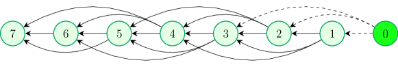
Figure 1: One example of MPF communication topology with $r_{1}=1,r_{2}=2$ and $r_{i}=r=3,i\in\textbf{I}_{3}^{7}$ based on Assumption 2.

TABLE I: Model Parameters

$N$	$d$	$\tau$	$\bar{h}$	$\bar{r}$	$v_{0}$	$A_{0}$	$\bar{\omega}_{0}$
7	5 $m$	0.5 s	0.6 s	3	$20$ $m/s$	$10$ $m/s^{2}$	1 $rad/s$

In the following, we give two scenarios with and without time headway $h$ minimization.

V-A Heuristic searching algorithm for controller parameters with fixed time headway in Sec. IV-E

V-A1 Condition (54) is satisfied

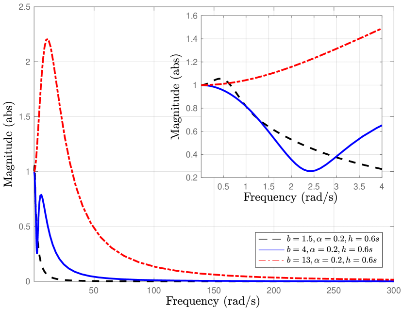
i The Bode plot of the original string stability condition (40) with different values of $b$ with $\alpha=0.2,h=0.6s$.

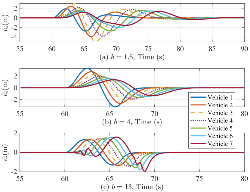
ii Platooning string stability performance comparison for different values of $b$ with $\alpha=0.2,h=0.6s$.

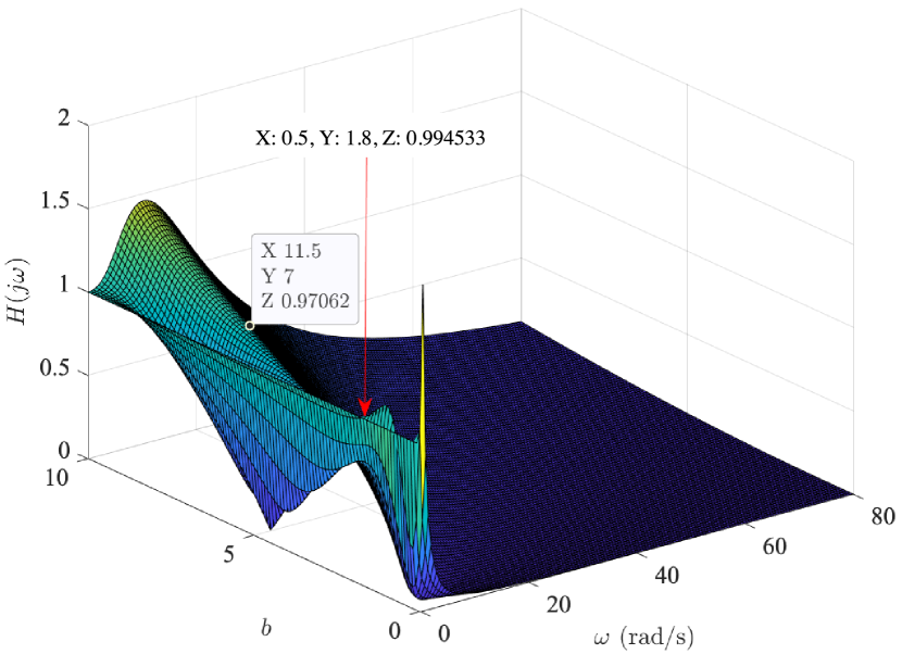
iii The relationship between $\left\|H(j\omega)\right\|_{\infty}$ and $b$ when $\alpha=0.2$.

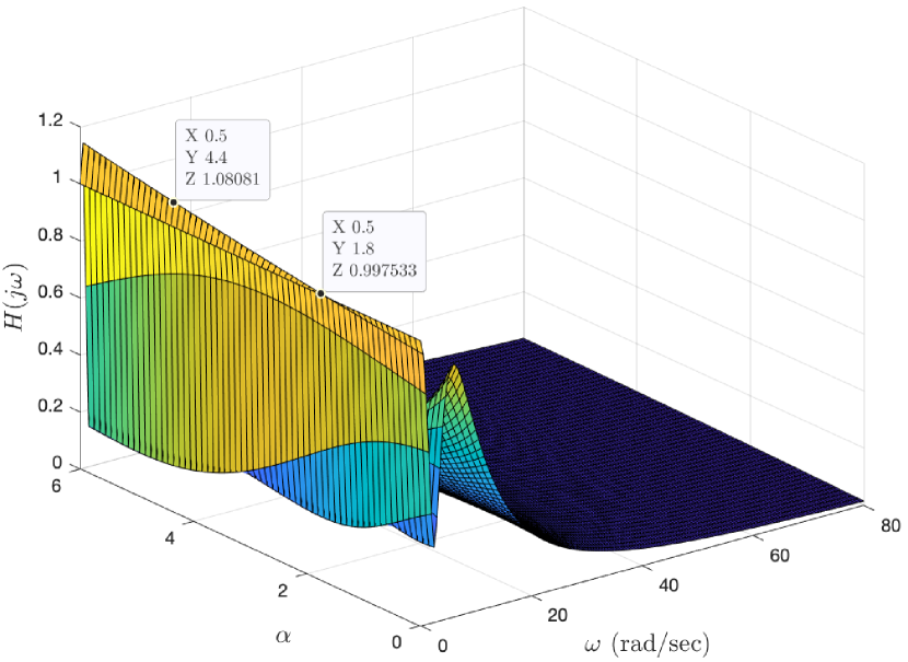
iv The relationship between $\left\|H(j\omega)\right\|_{\infty}$ and $\alpha$ when $b=4$.

Figure 2: Heuristic searching algorithm validation for controller parameters with fixed time headway in Sec. V-A1.

Based on $r=3$ and $\tau=0.5$, we fix the time headway as $h=\bar{h}=0.6s$. From the complimentary rule (56) in step ii, if we design $\alpha=0.2$, then, the main rule (55) in step i becomes $2.49\leq b<10$. Based on guidelines, we design $b=4$. We verify $\{\mathrm{W_{4}},\mathrm{W_{6}},\mathrm{W_{8}}\}>0$ in (54) as $\mathrm{W_{2}}=2621.4,\mathrm{W_{4}}=13476,\mathrm{W_{6}}=5140.5,\mathrm{W_{8}}=22.84$ and $\mathrm{W_{8}}+\mathrm{W_{10}}\omega^{2}\geq 0$ for $\omega\in[0,\omega_{0}],\omega_{0}=1.9930$ with $\mathrm{W_{10}}=-5.75$. It is worthy noting here that it does not mean the transformed string stability condition (53a) is only available for $\omega\in[0,\omega_{0}],$ as we also have $\{\mathrm{W_{2}},\mathrm{W_{4}},\mathrm{W_{6}}\}>0$. However, the calculation for deciding the exact range for $\omega$ with all $\{\mathrm{W_{2}},\mathrm{W_{4}},\mathrm{W_{6}}\}$ included would become very complicated as we can see in (53a). And this is the reason we use step iv to finally and formally confirm our designed parameters $\alpha=0.2$ and $b=4$ as in the Fig. 2 (i) which means the string stability is guaranteed.

In order to validate our results, we provide comparison simulations, e.g., by keeping $\alpha=0.2$, we give two other choices of $b$ ($b=1.5$ and $b=13$) which is out of the value range: $2.49\leq b<10$ from the main rule (55). The Bode plot of different values of parameter $b$ in Fig. 2 (i) demonstrates that the case of $b=4$ guarantees the string stability while the other two cases do not, which shows the effectiveness of our proposed heuristic searching algorithm (parameter setting mechanism) in Sec. IV-E.

Furthermore, to visualize the string stable performance, Fig. 2 (ii) describes the predecessor-follower platooning spacing error plot. One can see only Fig. 2 (ii) (b) demonstrates that the platooning is string stable as the error does not amplify from vehicle $1$ to $7$, while the scenarios of $b=1.5$ in (a) and $b=13$ in (c) are not. The string stability performance shown in Fig. 2 (ii) is in accordance with the Bode plot in Fig. 2 (i).

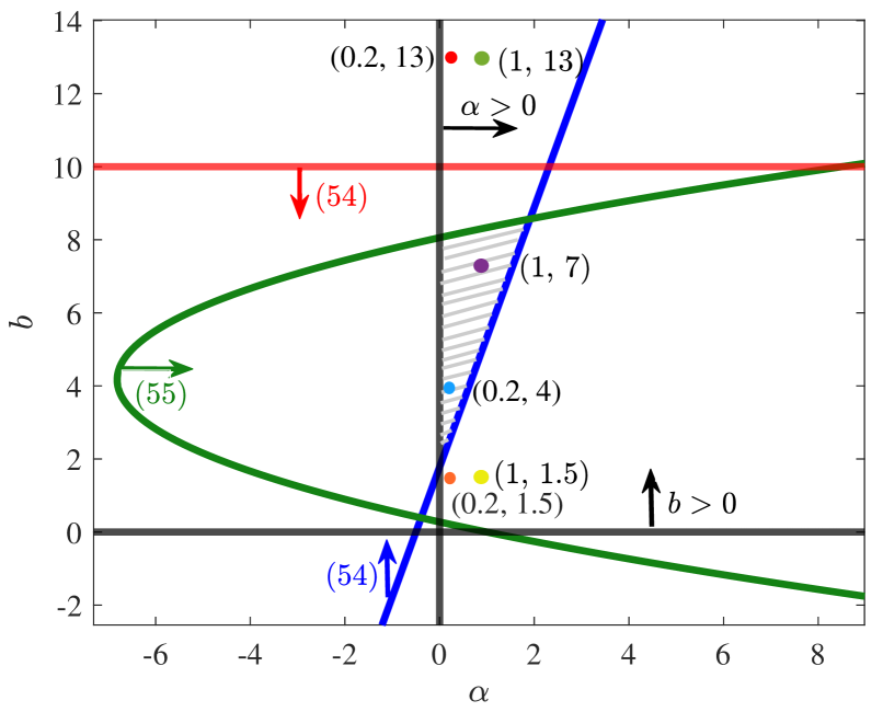
i The feasible region for parameters $\alpha$ and $b$ given $h=0.6s$.

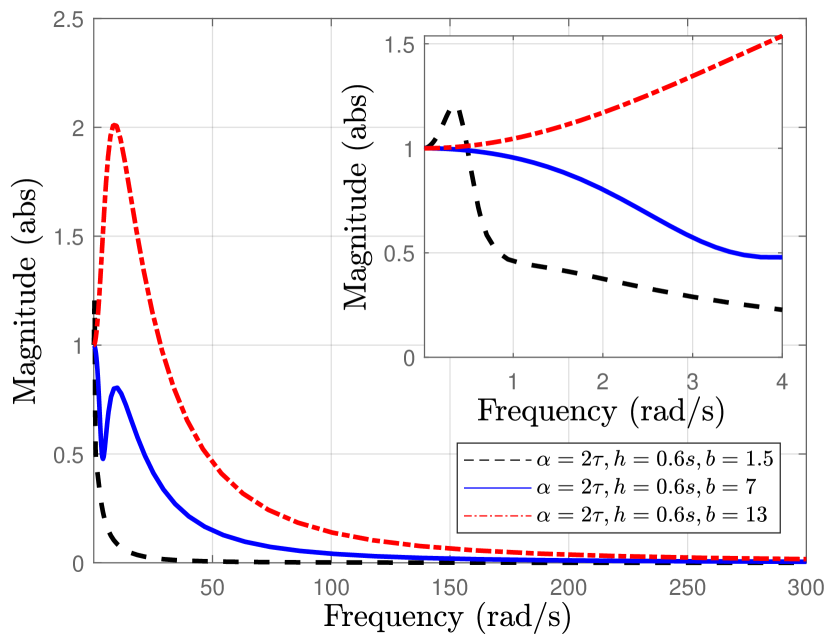
ii The Bode plot with different values of $b$ with $\alpha=2\tau,h=0.6s$.

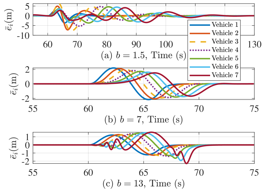
iii Platooning comparison for different values of $b$ with $\alpha=2\tau,h=0.6s$.

Figure 3: Heuristic searching algorithm validation for controller parameters with fixed time headway in Sec. V-A2.

It is worth noting that all the errors converge to zero in Fig. 2 (ii) (a), (b), (c) and that the error of vehicle $1$ converges to zero first, then that of vehicle $2$, and so on, and finally the error of the last vehicle (vehicle $7$) converges to zero, which verifies Theorem 1.

Blind search method for controller parameters: As we state in Remark 9, the parameter setting mechanism in Sec. IV-E is neither sufficient nor necessary to guarantee the platoon string stability, and is rather a heuristic searching algorithm for possible solutions. If we do not use the above mechanism, i.e., we do not have any information or guidelines about how to design $\alpha$ and $b$, then a blind search method (i.e., guess the values of $\alpha,b$ randomly and then tune them) can be adopted along with maybe many trials and errors.

The blind search method is a numerical analysis method (e.g., meshgrid and surf functions in MATLAB) to get the relationship among $\left\|H(j\omega)\right\|_{\infty}$ and parameters $\alpha,b$ in (40) To decide the relationship among $\left\|H(j\omega)\right\|_{\infty}$ and parameters $\alpha,b$, one solution is to use the command scatter3 in MATLAB to have a 4-D map which is not expressive to read. Instead, we choose to use commands meshgrid and surf to have 3-D maps which is more direct and expressive.

First, assume we are lucky to set $\alpha=0.2$ without many trials, Fig. 2 (iii) shows that $1.8\leq b\leq 7$ is a decent choice for platooning string stability. One can see this range is different from the range $2.49\leq b<10$ (or even $2.49\leq b<8.33$ considering the complimentary rule (56) with $b<5/h$), which verifies the above mechanism is neither sufficient nor necessary. However, they do have a quite large overlapped range $2.49\leq b\leq 7$ which accounts for $86.7\%$ of $1.8\leq b\leq 7$ and $77.2\%$ of $2.49\leq b<8.33$ respectively, demonstrating the effectiveness of the above mechanism.

Then, we choose $b=4$ and Fig. 2 (iv) shows $0<\alpha\leq 1.8$ is acceptable. Therefore, the choice of $(b=4,\alpha=0.2)$ is good to satisfy the string stability condition (40) given the time headway $h$ is fixed. Fig. 3 (i) shows the feasible region from the proposed controller parameter ( $\alpha$ and $b$) design mechanism given $h=0.6s$, which also validates the above analysis.

V-A2 Condition (54) is not satisfied

Same as the above example, from the complimentary rule (56) in step ii, if we design $\alpha=2\tau$, then, the main rule (55) in step i becomes $5.33\leq b<10$; we design $b=7$. Then, we have $\mathrm{W_{2}}=-1.1924e^{8}<0,\mathrm{W_{4}}=-5.5913e^{6}<0,\mathrm{W_{6}}=1.1837e^{5}>0,\mathrm{W_{8}}=2.5167e^{3}>0$, which means condition (54) is not satisfied. However, from Fig. 3 (ii) we can see that by designing $\alpha=2\tau$ and $b=7$, the string stability can be guaranteed, which is also confirmed by Fig. 3 (iii).

This example verifies Remark 9 that rules (55) and (56) are only necessary, but not sufficient for condition (54). It confirms that the Bode plot of the original string stability condition (40) is the formal and final measurement for string stability verification. Also, this example demonstrates the effectiveness of our proposed rules (55) and (56) for guaranteeing the string stability of vehicle platooning.

Remark 11

The above two examples in Sec. V-A shows that given a fixed time headway $h$, there exist multiple solutions of $\alpha$ and $b$ to guarantee the string stability of vehicle platooning.

V-B Algorithm 1 for controller parameters with time headway minimization in Sec. IV-F

Here, the same model parameters are used here, except that we set $\alpha=2\tau$ and use Algorithm 1 to minimize $h$ from $h=\bar{h}=0.6s$. Finally, we arrive at $h=0.112s,b=10$ from $h=0.6s,0.3s,0.15s,0.075s,0.112s$. Fig. 4 demonstrates the effectiveness and efficacy of proposed Algorithm 1 for obtaining the minimum time headway $h$.

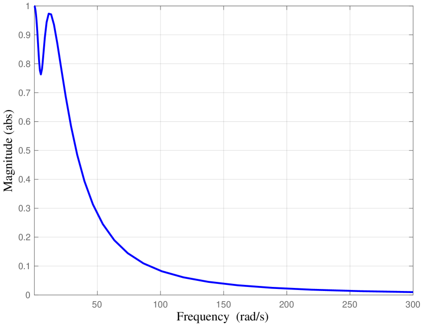
i The Bode plot with $h=0.112s,b=10$ and $\alpha=2\tau$.

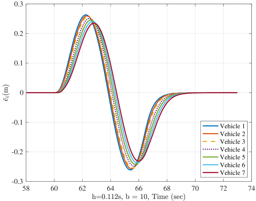
ii The corresponding platooning string stability performance.

Figure 4: Algorithm 1 for controller parameters with time headway minimization in Sec. V-B.

Remark 12

One can observe that values of $\alpha$ in the above two examples in Secs. V-A and V-B are different. The reason is that Algorithm 1 verified in Sec. V-B is by fixing $\alpha=2\tau$ to minimize the value of $h$. Actually, given a fixed $h$, $\alpha$ can have different values; and this is the heuristic searching algorithm in Sec. V-A demonstrates. To sum up, the objective of the heuristic searching algorithm is to design controller parameters $\alpha$ and $b$ given a fixed $h$ while the objective of Algorithm 1 is to minimize the value of $h$ by fixing $\alpha=2\tau$. To analyze the relationship among $\alpha,b$ and $h$ directly without fixing one value would be an interesting direction in the future.

VI Conclusions and Future Directions

VI-A Conclusions

The vehicle platooning with a leader whose speed is time-varying is studied in this work by designing an observer-based controller under a directed MPF IFT. The observer’s matrix format is firstly proposed to guarantee the internal stability of the platoon system. Subsequently, by designing a specific observer parameter matrix, this observer turns out to have a third-order integrator dynamics (scalar format) which is utilized to derive the string stability conditions for designing observer and controller parameters. To deduce the string stability criterion, instead of calculating the derivatives of predecessor-follower spacing error directly which is also difficult, a new variable which is linked to that spacing error is proposed with its derivatives calculated instead till reaching the string stability criterion. To design controller parameters from the above string stability criterion, a new parameter design mechanism given a fixed time headway is proposed to have a heuristic searching algorithm; furthermore, a bisection-like algorithm is incorporated into the above algorithm to obtain the minimum available value of the time headway by fixing one controller parameter. The validity of our results is demonstrated through comparison examples.

VI-B Future Directions

In this work, though the leader vehicle’s speed is time-varying, its dynamics is autonomous. Investigating the non-autonomous dynamics (i.e., the leader has non-zero input) is more realistic and challenging. Another interesting direction is the study of the platoon system when the communication links are unreliable and they cause delays and packet losses. Investigating nonlinear spacing policies that allow vehicles to be added to the platoon system is also one considered direction.

References

- [1] W. Levine and M. Athans, “On the optimal error regulation of a string of moving vehicles,” IEEE Trans. Autom. Control, vol. 11, no. 3, pp. 355–361, 1966.
- [2] J. Ploeg, N. Van De Wouw, and H. Nijmeijer, “Lp string stability of cascaded systems: Application to vehicle platooning,” IEEE Trans. Control Syst. Technol., vol. 22, no. 2, pp. 786–793, 2013.
- [3] P. Seiler, A. Pant, and K. Hedrick, “Disturbance propagation in vehicle strings,” IEEE Trans. Autom. Control, vol. 49, no. 10, pp. 1835–1842, 2004.
- [4] R. H. Middleton and J. H. Braslavsky, “String instability in classes of linear time invariant formation control with limited communication range,” IEEE Trans. Autom. Control, vol. 55, no. 7, pp. 1519–1530, 2010.
- [5] Y. Bian, Y. Zheng, W. Ren, S. E. Li, J. Wang, and K. Li, “Reducing time headway for platooning of connected vehicles via V2V communication,” Transport. Res. Part C: Emerg. Technol., vol. 102, pp. 87–105, 2019.
- [6] S. Feng, Y. Zhang, S. E. Li, Z. Cao, H. X. Liu, and L. Li, “String stability for vehicular platoon control: Definitions and analysis methods,” Ann. Rev. Control, vol. 47, pp. 81 – 97, 2019.
- [7] S. Stüdli, M. Seron, and R. Middleton, “From vehicular platoons to general networked systems: String stability and related concepts,” Ann. Rev. Control, vol. 44, pp. 157 – 172, 2017.
- [8] J. Monteil, G. Russo, and R. Shorten, “On L string stability of nonlinear bidirectional asymmetric heterogeneous platoon systems,” Automatica, vol. 105, pp. 198–205, 2019.
- [9] P. Barooah and J. P. Hespanha, “Error amplification and disturbance propagation in vehicle strings with decentralized linear control,” in Proc. 44th IEEE Conf. Dec. Control. IEEE, 2005, pp. 4964–4969.
- [10] G. J. Naus, R. P. Vugts, J. Ploeg, M. J. van De Molengraft, and M. Steinbuch, “String-stable CACC design and experimental validation: A frequency-domain approach,” IEEE Trans. Veh. Technol., vol. 59, no. 9, pp. 4268–4279, 2010.
- [11] C. Flores and V. Milanés, “Fractional-order-based ACC/CACC algorithm for improving string stability,” Transport. Res. Part C: Emerg. Technol., vol. 95, pp. 381–393, 2018.
- [12] L. Peppard, “String stability of relative-motion pid vehicle control systems,” IEEE Trans. Autom. Control, vol. 19, no. 5, pp. 579–581, 1974.
- [13] S. Sheikholeslam and C. A. Desoer, “Longitudinal control of a platoon of vehicles,” in Proc. Amer. Control Conf. (ACC). IEEE, 1990, pp. 291–296.
- [14] S. Feng, Y. Zhang, S. E. Li, Z. Cao, H. X. Liu, and L. Li, “String stability for vehicular platoon control: Definitions and analysis methods,” Ann. Rev. Control, vol. 47, pp. 81–97, 2019.
- [15] B. Besselink and K. H. Johansson, “String stability and a delay-based spacing policy for vehicle platoons subject to disturbances,” IEEE Trans. Autom. Control, vol. 62, no. 9, pp. 4376–4391, 2017.
- [16] L. Xiao and F. Gao, “Practical string stability of platoon of adaptive cruise control vehicles,” IEEE Trans. Intell. Transp. Syst., vol. 12, no. 4, pp. 1184–1194, 2011.
- [17] E. Abolfazli, B. Besselink, and T. Charalambous, “Reducing time headway in platoons under the MPF topology when using sensors and wireless communications,” in Proc. 59th IEEE Conf. Dec. Control. IEEE, 2020, pp. 2823–2830.
- [18] ——, “On time headway selection in platoons under the MPF topology in the presence of communication delays,” IEEE Trans. Intell. Transport. Syst., pp. 1–14, 2021.
- [19] A. Ali, G. Garcia, and P. Martinet, “The flatbed platoon towing model for safe and dense platooning on highways,” IEEE Trans. Intell. Transp. Syst. Mag., vol. 7, no. 1, pp. 58–68, 2015.
- [20] G. Rödönyi, “An adaptive spacing policy guaranteeing string stability in multi-brand ad hoc platoons,” IEEE Trans. Intell. Transport. Syst., vol. 19, no. 6, pp. 1902–1912, 2017.
- [21] J. Hu, P. Bhowmick, F. Arvin, A. Lanzon, and B. Lennox, “Cooperative control of heterogeneous connected vehicle platoons: An adaptive leader-following approach,” IEEE Robot. Autom. Let., vol. 5, no. 2, pp. 977–984, 2020.
- [22] A. Khalifa, O. Kermorgant, S. Dominguez, and P. Martinet, “An observer-based longitudinal control of car-like vehicles platoon navigating in an urban environment,” in Proc. 58th IEEE Conf. Dec. Control. IEEE, 2019, pp. 5735–5741.
- [23] W. Jiang, E. Abolfazli, and T. Charalambous, “Observer-based control for vehicle platooning with a leader of varying velocity,” in European Control Conf., 2021, pp. 1–8.
- [24] E. Kayacan, “Multiobjective control for string stability of cooperative adaptive cruise control systems,” IEEE Trans. Intell. Veh., vol. 2, no. 1, pp. 52–61, 2017.
- [25] H. Chehardoli and M. R. Homaeinezhad, “Third-order safe consensus of heterogeneous vehicular platoons with MPF network topology: constant time headway strategy,” P I Mech. Eng. D-J. Aut., vol. 232, no. 10, pp. 1402–1413, 2018.
- [26] M. di Bernardo, P. Falcone, A. Salvi, and S. Santini, “Design, analysis, and experimental validation of a distributed protocol for platooning in the presence of time-varying heterogeneous delays,” IEEE Trans. Control Syst. Technol., vol. 24, no. 2, pp. 413–427, 2016.
- [27] J. Ploeg, E. Semsar-Kazerooni, G. Lijster, N. van de Wouw, and H. Nijmeijer, “Graceful degradation of CACC performance subject to unreliable wireless communication,” in Proc. 16th Int. Conf. Intell. Transp. Syst. (ITSC). IEEE, 2013, pp. 1210–1216.
- [28] W. Jiang, Y. Chen, and T. Charalambous, “Consensus of general linear multi-agent systems with heterogeneous input and communication delays,” IEEE Control Syst. Lett., vol. 5, no. 3, pp. 851–856, 2021.
- [29] E. Shaw and J. K. Hedrick, “String stability analysis for heterogeneous vehicle strings,” in Proc. Amer. Control Conf. (ACC). IEEE, 2007, pp. 3118–3125.
- [30] R. S. Barbosa, “Vehicle vibration response subjected to longwave measured pavement irregularity,” J. Mech. Eng. Aut., vol. 2, no. 2, pp. 17–24, 2012.