Beyond Linear Algebra

Abstract

Our title challenges the reader to venture beyond linear algebra in designing models and in thinking about numerical algorithms for identifying solutions. This article accompanies the author’s lecture at the International Congress of Mathematicians 2022. It covers recent advances in the study of critical point equations in optimization and statistics, and it explores the role of nonlinear algebra in the study of linear PDE with constant coefficients.

1 Introduction

Linear algebra is ubiquitous in the mathematical universe. It plays a foundational role for many models in the sciences and engineering, and its numerical methods are a driving force behind today’s technologies. The power of linear algebra stems from our ability, honed through the practice of calculus, to approximate nonlinear shapes by linear spaces.

Yet, the world is nonlinear. Nonlinear equations are a natural ingredient in mathematical models for the real world. In our view, the true nonlinear nature of a phenomenon should be respected as long as possible. We argue against the common practice of passing to a linear approximation immediately. Of course, in the final step of implementing scalable algorithms, one will always employ the powerful tools of numerical linear algebra. However, in the early phase of exploring and designing a model, there is significant benefit in going beyond linear algebra. Mathematical fields such as algebraic geometry, algebraic topology, combinatorics, commutative algebra or representation theory furnish practical tools.

The growing awareness of theoretical mathematics in applications has led to a new field called Nonlinear Algebra. The textbook [32] offers foundations for interested students. The aim of this lecture is to introduce research trends and discuss a few recent results. At the core of many problems lies the study of subsets of $\mathbb{R}^{n}$ that are defined by polynomials:

(1.1) $$\bigl{\{}\,x\in\mathbb{R}^{n}:f_{1}(x)=\cdots=f_{k}(x)=0,g_{1}(x)\geq 0,\ldots,g_{l}(x)\geq 0,h_{1}(x)>0,\ldots,h_{m}(x)>0\bigr{\}}.$$

The set (1.1) is a basic semialgebraic set. The Positivstellensatz [32, Theorem 6.14] gives a criterion for deciding whether this set is empty. This seemingly theoretical criterion has become a practical numerical method, thanks to sums of squares [32, §12.3] and semidefinite programming [7]. In addition to this, there are symbolic algorithms for real algebraic geometry (cf. [5]). So, the user has a wide range of choices for working with semialgebraic sets.

In this article we disregard the inequalities in (1.1) and retain the equations only:

(1.2) $$X\,\,=\,\,\bigl{\{}\,x\in\mathbb{R}^{n}:f_{1}(x)=\cdots=f_{k}(x)=0\bigr{\}}.$$

This is a real algebraic variety. We wish to answer questions about $X$ by reliable numerical computations, in particular using tools such as Bertini [6] or HomotopyContinuation.jl [10]. We focus on questions that are addressed by solving auxiliary polynomial systems with finitely many solutions, where the number of complex solutions can be determined a priori.

In Section 2 that number is the Euclidean distance degree (ED degree) of $X$. This governs the following question: given $u\in\mathbb{R}^{n}\backslash X$, which point in $X$ is nearest to $u$ in Euclidean distance? We derive the critical equations of this optimization problem (2.1), and we consider all solutions to these equations, both real and complex. These include all local minima and local maxima. Theorem 2.5 expresses the ED degree in terms of the polar degrees of $X$. Knowing these invariants allows us to find all critical points numerically, along with a proof of correctness [9]. We ask our nearest point question also for other norms, notably those given by a polytope. The polar degrees appear again, in Proposition 2.9.

Section 3 concerns algebraic varieties $X$ that serve as models in statistics. Their points represent probability distributions. We focus on models for Gaussian distributions and discrete distributions. In these two scenarios, the ambient space $\mathbb{R}^{n}$ in (1.2) is replaced by the positive-definite cone $\text{PD}_{n}$ and by the probability simplex $\Delta_{n}$. Given any data set, we wish to ascertain whether $X$ is an appropriate model. To this end, maximum likelihood estimation (MLE) is used. This optimization problem is stated explicitly in (3.2) and (3.7), and we employ nonlinear algebra [32] in addressing it. The number of complex critical points is the maximum likelihood degree (ML degree) of the model $X$. Theorem 3.7 relates this to the Euler characteristic of the underlying very affine variety. We apply this theory to a class of models arising in particle physics, namely the configuration space of $m$ labeled points in general position in $\mathbb{P}^{k-1}$. Known ML degrees for these models are given in Theorem 3.14.

In Section 4, we turn to an analytic interpretation of the polynomial system in (1.2). The unknowns $x_{1},\ldots,x_{n}$ are replaced by differential operators $\frac{\partial}{\partial z_{1}},\ldots,\frac{\partial}{\partial z_{n}}$, and the polynomials $f_{1},\ldots,f_{k}$ are viewed as linear partial differential equations (PDE) with constant coefficients. The variety $X$ is replaced by the space of functions $\phi(z_{1},\ldots,z_{n})$ that are solutions to the PDE. That space is typically infinite-dimensional. Our task is to compute it. Algorithms are based on differential primary decompositions [2, 18, 17]. We also study linear PDE for vector-valued functions. These are expressed by modules over a polynomial ring.

This article accompanies a lecture to be given in July 2022 at the International Congress of Mathematicians in St. Petersburg. It encourages mathematical scientists to employ polynomials in designing models and in thinking about numerical algorithms. Sections 2 and 3 are concerned with critical point equations in optimization and statistics. Section 4 offers a glimpse on how nonlinear algebra interfaces with the study of linear PDE.

2 Nearest Points on Algebraic Varieties

We consider a model $X$ that is given as the zero set in $\mathbb{R}^{n}$ of a collection $\{f_{1},\ldots,f_{k}\}$ of nonlinear polynomials in $n$ unknowns $x_{1},\ldots,x_{n}$. Thus, $X$ is a real algebraic variety. We assume that $X$ is irreducible, that $I_{X}=\langle f_{1},\ldots,f_{k}\rangle$ is its prime ideal, and that the set of nonsingular real points is Zariski dense in $X$. The $k\times n$ Jacobian matrix $\mathcal{J}=(\partial f_{i}/\partial x_{j})$ has rank at most $c$ at any point $x\in X$, where $c=\text{codim}(X)$, and $x$ is nonsingular on $X$ if the rank is exactly $c$. Explanations of these hypotheses are found in Chapter 2 of the textbook [32].

The following optimization problem arises in many applications. Given a data point $u\in\mathbb{R}^{n}\backslash X$, compute the distance to the model $X$. Thus, we seek a point $x^{*}$ in $X$ that is closest to $u$. The answer depends on the chosen metric. One might choose the Euclidean distance, a $p$-norm [29], or polyhedral norms, such as those arising in optimal transport [15]. In all of these cases, the solution $x^{*}$ can be found by solving a system of polynomial equations.

We begin by discussing the Euclidean distance (ED) problem, which is as follows:

(2.1) $$\text{minimize}\,\,\sum_{i=1}^{n}(x_{i}-u_{i})^{2}\,\,\text{subject to}\,\,\,x\in X.$$

We now derive the critical equations for (2.1). The augmented Jacobian matrix $\mathcal{AJ}$ is the $(k+1)\times n$ matrix obtained by placing the row $(x_{1}-u_{1},\ldots,x_{n}-u_{n})$ atop the Jacobian matrix $\mathcal{J}$. We form the ideal generated by its $(c+1)\times(c+1)$ minors, we add the ideal of the model $I_{X}$, and we then saturate [19, (2.1)] that sum by the ideal of $c\times c$ minors of $\mathcal{J}$. The result is the critical ideal $\mathcal{C}_{X,u}$ of the model $X$ with respect to the data $u$. The variety of $\mathcal{C}_{X,u}$ is the set of critical points of (2.1). For random data $u$, this variety is finite and it contains the optimal solution $x^{*}$, provided the latter is attained at a nonsingular point of $X$.

The algebro-geometric approach to the ED problem was pioneered in a project with Draisma, Horobeţ, Ottaviani and Thomas [19]. That article introduced the ED degree of $X$. This is the cardinality of the complex algebraic variety in $\mathbb{C}^{n}$ defined by the critical ideal $\mathcal{C}_{X,u}$. The ED degree of a model $X$ measures the difficulty of solving the ED problem for $X$.

Example 2.1 (Space curves).

Fix $n=3$ and let $X$ be the curve in $\mathbb{R}^{3}$ defined by two general polynomials $f_{1}$ and $f_{2}$ of degrees $d_{1}$ and $d_{2}$ in $x_{1},x_{2},x_{3}$. The augmented Jacobian matrix is

(2.2) $$\mathcal{AJ}\,\,=\,\,\,\,\begin{pmatrix}x_{1}-u_{1}&&x_{2}-u_{2}&&x_{3}-u_{3}\\ \partial f_{1}/\partial x_{1}&\,\,\,&\partial f_{1}/\partial x_{2}&\,\,\,&\partial f_{1}/\partial x_{3}\\ \partial f_{2}/\partial x_{1}&\,\,\,&\partial f_{2}/\partial x_{2}&\,\,\,&\partial f_{2}/\partial x_{3}\\ \end{pmatrix}.$$

For random data $u\in\mathbb{R}^{3}$, the ideal $\,\mathcal{C}_{X,u}=\bigl{\langle}f_{1},\,f_{2},\,\text{det}(\mathcal{AJ})\bigr{\rangle}\,$ has $d_{1}d_{2}(d_{1}+d_{2}-1)$ zeros in $\mathbb{C}^{3}$, by Bézout [32, Theorem 2.16]. Hence the ED degree of $X$ equals $d_{1}d_{2}(d_{1}+d_{2}-1)$. This can also be seen using the general formula from algebraic geometry in [19, Corollary 5.9]. If $X$ is a general smooth curve of degree $d$ and genus $g$, then $\text{EDdegree}(X)=3d+2g-2$. The above curve in $3$-space has degree $d=d_{1}d_{2}$ and genus $g=d_{1}^{2}d_{2}/2+d_{1}d_{2}^{2}/2-2d_{1}d_{2}+1$.

Here is a general upper bound on the ED degree in terms of the given polynomials.

Proposition 2.2.

Let $X$ be a variety of codimension $c$ in $\mathbb{R}^{n}$ whose ideal $I_{X}$ is generated by polynomials $f_{1},f_{2},\ldots,f_{c},\ldots,f_{k}\,$ of degrees $\,d_{1}\geq d_{2}\geq\cdots\geq d_{c}\geq\cdots\geq d_{k}$. Then

(2.3) $$\text{EDdegree}(X)\,\,\,\leq\,\,\,\,d_{1}d_{2}\cdots d_{c}\cdot\!\!\!\!\!\!\!\!\!\!\!\!\sum_{i_{1}+i_{2}+\cdots+i_{c}\leq n-c}\!\!\!\!\!(d_{1}-1)^{i_{1}}(d_{2}-1)^{i_{2}}\cdots(d_{c}-1)^{i_{c}}.$$

Equality holds when $X$ is a generic complete intersection of codimension $c$ (hence $c=k$).

This appears in [19, Proposition 2.6]. We can derive it as follows. Bézout’s Theorem ensures that the degree of the variety $X$ is at most $d_{1}d_{2}\cdots d_{c}$. The entries in the $i$th row of the matrix $\mathcal{AJ}$ are polynomials of degrees $d_{i}-1$. The degree of the variety of $(c+1)\times(c+1)$ minors of $\mathcal{AJ}$ is at most the sum in (2.3). The intersection of that variety with $X$ is our set of critical points, and the cardinality of that set is bounded by the product of the two degrees. Generically, that intersection is a complete intersection and the inequality (2.3) is attained.

Formulas or a priori bounds for the ED degree are important when studying exact solutions to the optimization problem (2.1). The paradigm is to compute all complex critical points, by either symbolic or numerical methods, and to then extract one’s favorite real solutions among these. This leads, for instance, to all local minima in (2.1). The ED degree is an upper bound on the number of real critical points, but this bound is generally not tight.

Example 2.3.

Consider the case $n=2,c=1,d_{1}=4$ in Proposition 2.2, where $X$ is a quartic curve in the plane $\mathbb{R}^{2}$. The number of complex critical points is $\textrm{EDdegree}(X)=16$. But, they cannot be all real. For an illustration, consider the Trott curve $X=V(f)$, defined by

$$f\,\,=\,\,144(x_{1}^{4}+x_{2}^{4})\,-\,225(x_{1}^{2}+x_{2}^{2})\,+\,350x_{1}^{2}x_{2}^{2}\,+\,81.$$

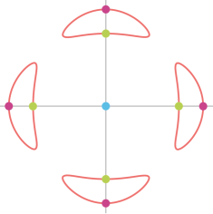
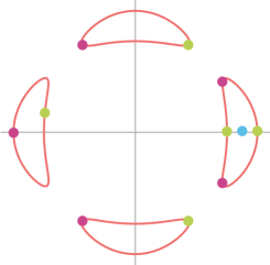
Figure 1: ED problems on the Trott curve: configurations of eight (left) or ten (right) critical points.

For general data $u=(u_{1},u_{2})$ in $\mathbb{R}^{2}$, we find $16$ complex solutions to the critical equations $f=\frac{\partial f}{\partial x_{2}}(x_{1}-u_{1})-\frac{\partial f}{\partial x_{1}}(x_{2}-u_{2})=0$. For $u$ near the origin, eight of them are real. For $u=\bigl{(}\frac{7}{8},\frac{1}{100}\bigr{)}$, which is inside the rightmost oval, there are $10$ real critical points. The two scenarios are shown in Figure 1. Local minima are green, while local maxima are purple. For $u=(2,\frac{1}{100})$, to the right of the rightmost oval, the number of real critical points is $12$.

In general, our task is to compute the zeros of the critical ideal $C_{X,u}$. Algorithms for this computation can be either symbolic or numerical. Symbolic methods usually rest on the construction of a Gröbner basis, to be followed by a floating point computation to extract the solutions. In recent years, numerical methods have become increasingly popular. These are based on homotopy continuation. Two notable packages are Bertini [6] and HomotopyContinuation.jl [10]. The ED degree is important here because it indicates how many paths need to be tracked to solve (2.1). We next illustrate current capabilities.

Example 2.4.

Suppose $X$ is defined by $c=k=3$ random polynomials in $n=7$ variables, for a range of degrees $d_{1},d_{2},d_{3}$. The table below lists the ED degree in each case, and the times used by HomotopyContinuation.jl to compute and certify all critical points in $\mathbb{C}^{7}$.

$$\begin{matrix}d_{1}\,d_{2}\,d_{3}&\quad 3\,2\,2\quad&\quad 3\,3\,2\quad&\quad 3\,3\,3\quad&\quad 4\,2\,2\quad&\quad 4\,3\,2\quad&\quad 4\,3\,3\quad&\quad 4\,4\,2\quad&\quad 4\,4\,3\quad\\ \ \textrm{EDdegree}&\quad 1188&\quad 3618&\quad 9477&\quad 4176&\quad 10152&\quad 23220&\quad 23392&\quad 49872\\ \textrm{Solving (sec)}&\quad 3.849&\quad 21.06&\quad 61.51&\quad 31.51&\quad 103.5&\quad 280.0&\quad 351.5&\quad 859.3\\ \!\textrm{Certifying (sec)}\!\!\!\!&\quad 0.390&\quad 1.549&\quad 4.653&\quad 2.762&\quad 7.591&\quad 17.16&\quad 21.65&\quad 50.07\\ \end{matrix}$$

Here we represent $C_{X,u}$ by a system of $10$ equations in $10$ variables. In addition to the three equations $f_{1}=f_{2}=f_{3}=0$ in $x_{1},\ldots,x_{7}$, we take the seven equations $(1,y_{1},y_{2},y_{3})\cdot\mathcal{AJ}=0$. Here $y_{1},y_{2},y_{3}$ are new variables. These ensure that the $4\times 7$ matrix $\mathcal{AJ}$ has rank $\leq 3$. In all cases the timings include the certification step [9] that proves correctness and completeness. These computations were performed using HomotopyContinuation.jl v2.5.6 on a 16 GB MacBook Pro with an Intel Core i7 processor working at 2.6 GHz. They suggest that our critical equations can be solved fast and reliably, with proof of correctness, when the ED degree is less than $50000$. For even larger numbers of solutions, success with numerical path tracking will depend on the specific structure of the problem. If the discriminant is well-behaved, then larger ED degrees are feasible. An example of this appears in [34, Table 1].

We next present a general formula for ED degrees in terms of projective geometry.

Theorem 2.5.

If $\,X$ meets both the hyperplane at infinity and the isotropic quadric transversally, then $\text{EDdegree}(X)$ equals the sum of the polar degrees of the projective closure of $X$.

The projective closure of $X\subset\mathbb{R}^{n}$ is its Zariski closure in complex projective space $\mathbb{P}^{n}$, which we will also denote by $X$. Theorem 2.5 appears in [19, Proposition 6.10]. The hypothesis is stated precisely in [19, equation (6.4)]. It holds for all $X$ after a general linear change of coordinates. We now explain what the polar degrees of a variety $X\subset\mathbb{P}^{n}$ are. Points $h$ in the dual projective space $(\mathbb{P}^{n})^{\vee}$ represent hyperplanes $\{x\in\mathbb{P}^{n}:h_{0}x_{0}+\cdots+h_{n}x_{n}=0\}$. We are interested in all pairs $(x,h)$ in $\mathbb{P}^{n}\times(\mathbb{P}^{n})^{\vee}$ such that $x$ is a nonsingular point of $X$ and $h$ is tangent to $X$ at $x$. The Zariski closure of this set is the conormal variety $N_{X}\subset\mathbb{P}^{n}\times(\mathbb{P}^{n})^{\vee}$.

It is known that $N_{X}$ has dimension $n-1$, and if $X$ is irreducible then so is $N_{X}$. The image of $N_{X}$ under projection onto the second factor is the dual variety $X^{\vee}$. The role of $x\in\mathbb{P}^{n}$ and $h\in(\mathbb{P}^{n})^{\vee}$ can be swapped. The following biduality relations [22, §I.1.3] hold:

$$N_{X}=N_{X^{\vee}}\quad\text{and}\quad(X^{\vee})^{\vee}=X.$$

The class of $N_{X}$ in the cohomology ring $H^{*}(\mathbb{P}^{n}{\times}(\mathbb{P}^{n})^{\vee}\!,\,\mathbb{Z})=\mathbb{Z}[s,t]/\langle s^{n+1},t^{n+1}\rangle$ has the form

$$[N_{X}]\,=\,\delta_{1}(X)s^{n}t\,+\,\delta_{2}(X)s^{n-1}t^{2}\,+\,\delta_{3}(X)s^{n-2}t^{3}\,+\,\cdots\,+\,\delta_{n}(X)st^{n}.$$

The coefficients $\delta_{i}(X)$ of this binary form are nonnegative integers, known as polar degrees.

Remark 2.6.

The polar degrees satisfy $\delta_{i}(X)=\#(N_{X}\,\cap\,(L\times L^{\prime}))$, where $L\subset\mathbb{P}^{n}$ and $L^{\prime}\subset(\mathbb{P}^{n})^{\vee}$ are general linear subspaces of dimensions $n+1-i\,$ and $\,i$ respectively. This geometric interpretation implies that $\delta_{i}(X)=0$ for $i<\text{codim}(X^{\vee})$ and for $i>\text{dim}(X)+1$.

Example 2.7.

Let $X$ be a general surface of degree $d$ in $\mathbb{P}^{3}$. Its dual $X^{\vee}$ is a surface of degree $d(d-1)^{2}$ in $(\mathbb{P}^{3})^{\vee}$. The conormal variety $N_{X}$ is a surface in $\mathbb{P}^{3}\times(\mathbb{P}^{3})^{\vee}$, with class

$$[N_{X}]\,\,\,=\,\,\,d(d-1)^{2}\,s^{3}t\,\,+\,\,d(d-1)\,s^{2}t^{2}\,\,+\,\,d\,st^{3}.$$

The sum of the three polar degrees equals $\text{EDdegree}(X)=d^{3}-d^{2}+d$; see Proposition 2.2.

Theorem 2.5 allows us to compute the ED degree for many interesting varieties, e.g. using Chern classes [19, Theorem 5.8]. This is relevant for applications in machine learning [11] which rest on low-rank approximation of matrices and tensors with special structure [33].

The discussion so far was restricted to the Euclidean norm. But, we can measure distances in $\mathbb{R}^{n}$ with any other norm $||\,\cdot\,||$. Our optimization problem (2.1) extends naturally:

(2.4) $$\text{minimize}\,\,||x-u||\,\,\text{subject to}\,\,\,x\in X.$$

The unit ball $B=\{x\in\mathbb{R}^{n}:||x||\leq 1\}$ is a centrally symmetric convex body. Conversely, every centrally symmetric convex body $B$ defines a norm, and we can paraphrase (2.4) as follows:

(2.5) $$\text{minimize}\,\,\lambda\,\,\text{subject to}\,\,\,\lambda\geq 0\,\,\text{and}\,\,(u+\lambda B)\,\cap\,X\,\,\not=\,\,\emptyset.$$

If the boundary of $B$ is smooth and algebraic then we express the critical equations as a polynomial system. This is derived as before, but we now replace the first row of the augmented Jacobian matrix $\mathcal{AJ}$ with the gradient of the map $\,\mathbb{R}^{n}\rightarrow\mathbb{R},\,x\mapsto||x-u||$.

Another case of interest arises when $||\cdot||$ is a polyhedral norm. This means that $B$ is a centrally symmetric polytope. Familiar examples of polyhedral norms are $||\cdot||_{\infty}$ and $||\cdot||_{1}$, where $B$ is the cube and the crosspolytope respectively. In optimal transport theory, one uses a Wasserstein norm [15] whose unit ball $B$ is the polar dual of a Lipschitz polytope.

To derive the critical equations, a combinatorial stratification of the problem is used, given by the face poset of the polytope $B$. Suppose that $X$ is in general position. Then $(u+\lambda^{*}B)\,\cap\,X\,=\,\{x^{*}\}$ is a singleton for the optimal value $\lambda^{*}$ in (2.5). The point $\frac{1}{\lambda^{*}}(x^{*}-u)$ lies in the relative interior of a unique face $F$ of the unit ball $B$. Let $L_{F}$ denote the linear span of $F$ in $\mathbb{R}^{n}$. We have $\text{dim}(L_{F})=\text{dim}(F)+1$. Let $\ell$ be any linear functional on $\mathbb{R}^{n}$ that attains its minimum over the polytope $B$ at the face $F$. We view $\ell$ as a point in $(\mathbb{P}^{n})^{\vee}$.

Lemma 2.8.

The optimal point $x^{*}$ in (2.4) is the unique solution to the optimization problem

(2.6) $$\text{Minimize}\,\,\,\ell(x)\,\,\,\text{subject to}\,\,x\in(u+L_{F})\cap X.$$

Proof.

The general position hypothesis ensures that $u+L_{F}$ intersects $X$ transversally, and $x^{*}$ is a smooth point of that intersection. Moreover, $x^{*}$ is a minimum of the restriction of $\ell$ to the variety $(u+L_{F})\cap X$. By our hypothesis, this linear function is generic relative to the variety, so the number of critical points is finite and the function values are distinct. ∎

The problem (2.6) amounts to linear programming over a real variety. We now determine the algebraic degree of this optimization task when $F$ is a face of codimension $i$.

Proposition 2.9.

Let $L$ be a general affine-linear space of codimension $i-1$ in $\mathbb{R}^{n}$ and $\ell$ a general linear form. The number of critical points of $\ell$ on $L\cap X$ is the polar degree $\delta_{i}(X)$.

Proof.

This result is [15, Theorem 5.1]. The number of critical points of a linear form is the degree of the dual variety $(L\cap X)^{\vee}$. That degree coincides with the polar degree $\delta_{i}(X)$. ∎

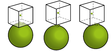
Figure 2: The cube is the $||\cdot||_{\infty}$ ball $\lambda^{*}B$ around the green point $u$. The variety $X$ is the sphere. The contact point $x^{*}$ is marked with a cross. The optimal face $F$ is a facet, a vertex, or an edge.

Example 2.10.

Consider (2.4) and (2.5) where $X$ is a general surface of degree $d$ in $\mathbb{R}^{3}$. The optimal face $F$ of the unit ball $B$ depends on the location of the data point $u$. This is shown for $d=2$ and $||\cdot||_{\infty}$ in Figure 2. The algebraic degree of the solution $x^{*}$ equals $\delta_{3}(X)=d$ if $\text{dim}(F)=0$, it is $\delta_{2}(X)=d(d-1)$ if $\text{dim}(F)=1$, and it is $\delta_{1}(X)=d(d-1)^{2}$ if $\text{dim}(F)=2$.

We conclude that the conormal variety $N_{X}$ and its cohomology class $[N_{X}]$ are key players when it comes to reliably solving the distance minimization problem for a variety $X$. The polar degrees $\delta_{i}(X)$ reveal precisely how many paths need to be tracked by numerical solvers like [6, 10] in order to find and certify [9] the optimal solution $x^{*}$ to (2.1) or (2.4).

3 Likelihood Geometry

The previous section was concerned with minimizing the distance from a given data point $u$ to a model $X$ that is described by polynomial equations. In what follows we consider the analogous problem in the setting of algebraic statistics [36], where the model $X$ represents a family of probability distributions. Distance to $u$ is replaced by the log-likelihood function.

The two scenarios of most interest for statisticians are Gaussian models and discrete models. We shall discuss them both, beginning with the Gaussian case. Let $\text{PD}_{n}$ denote the open convex cone of positive-definite symmetric $n\times n$ matrices. Given a mean vector $\mu\in\mathbb{R}^{n}$ and a covariance matrix $\Sigma\in\text{PD}_{n}$, the associated Gaussian distribution on $\mathbb{R}^{n}$ has the density

$$f_{\mu,\Sigma}(x)\,\,\,:=\,\,\,\frac{1}{\sqrt{(2\pi)^{n}\,\text{det}\,\Sigma}}\cdot\text{exp}\biggl{(}-\frac{1}{2}(x-\mu)^{T}\Sigma^{-1}(x-\mu)\biggr{)}.$$

We fix a model $Y\subset\mathbb{R}^{n}\times\text{PD}_{n}$ that is defined by polynomial equations in $(\mu,\Sigma)$. Suppose we are given $N$ samples $U^{(1)}\!,\ldots,U^{(N)}$ in $\mathbb{R}^{n}$. These are summarized in the sample mean $\bar{U}=\frac{1}{N}\sum_{i=1}^{N}U^{(i)}$ and in the sample covariance matrix $S=\frac{1}{N}\sum_{i=1}^{N}(U^{(i)}-\bar{U})(U^{(i)}-\bar{U})^{T}$. Given these data, the log-likelihood is the following function in the unknowns $(\mu,\Sigma)$:

(3.1) $$\ell(\mu,\Sigma)\quad=\quad-\frac{N}{2}\cdot\biggl{[}\,\text{log}\,\text{det}\,\Sigma\,\,+\,\,\text{trace}(S\Sigma^{-1})\,\,+\,\,(\bar{U}-\mu)^{T}\Sigma^{-1}(\bar{U}-\mu)\biggr{]}.$$

The task of likelihood inference is to minimize this function subject to $(\mu,\Sigma)\in Y$.

There are two extreme cases. First, consider a model where $\Sigma$ is fixed to be the identity matrix $\text{Id}_{n}$. Then $Y=X\times\{\text{Id}_{n}\}$ and we are supposed to minimize the Euclidean distance from the sample mean $\bar{U}$ to the variety $X$ in $\mathbb{R}^{n}$. This is precisely our problem (2.1).

We instead focus on the second case, the family of centered Gaussians, where $\mu$ is fixed at zero. The model has the form $\{0\}\times X$, where $X$ is a variety in the space $\text{Sym}_{2}(\mathbb{R}^{n})$ of symmetric $n\times n$ matrices. Following [36, Proposition 7.1.10], our task is now as follows:

(3.2) $$\text{Minimize the function}\,\,\,\,\Sigma\,\,\mapsto\,\,\text{log}\,\text{det}\,\Sigma\,\,+\,\,\text{trace}(S\,\Sigma^{-1})\quad\text{subject to}\,\,\Sigma\in X.$$

Using the concentration matrix $K=\Sigma^{-1}$, we can write this equivalently as follows:

(3.3) $$\text{Maximize the function}\,\,\,\,\Sigma\,\,\mapsto\,\,\text{log}\,\text{det}\,K\,\,-\,\,\text{trace}(S\,K)\quad\text{subject to}\,\,K\in X^{-1}.$$

Here the variety $X^{-1}$ is the Zariski closure of the set of inverses of all matrices in $X$.

The critical equations of the optimization problem (3.3) can be written as polynomials, since the partial derivatives of the logarithm are rational functions. These equations have finitely many complex solutions. Their number is the ML degree of the model $X^{-1}$.

Let $\mathcal{L}\subset\text{Sym}_{2}(\mathbb{R}^{n})$ be a linear space of symmetric matrices (LSSM), whose general element is assumed to be invertible. We are interested in the models $X^{-1}=\mathcal{L}$ and $X=\mathcal{L}$. It is convenient to use primal-dual coordinates $(\Sigma,K)$ to write the respective critical equations.

Proposition 3.1.

Fix an LSSM $\mathcal{L}$ and its orthogonal complement $\mathcal{L}^{\perp}$ for the inner product $\langle X,Y\rangle=\text{trace}(XY)$. The critical equations for the linear concentration model $X^{-1}=\mathcal{L}$ are

(3.4) $$K\in\mathcal{L}\,\,\,\text{and}\,\,\,K\Sigma=\text{Id}_{n}\,\,\,\text{and}\,\,\,\Sigma-S\in\mathcal{L}^{\perp}.$$

The critical equations for the linear covariance model $X=\mathcal{L}$ are

(3.5) $$\Sigma\in\mathcal{L}\,\,\,\text{and}\,\,\,K\Sigma=\text{Id}_{n}\,\,\,\text{and}\,\,\,KSK-K\in\mathcal{L}^{\perp}.$$

Proof.

This is well-known in statistics. For proofs see [35, Propositions 3.1 and 3.3]. ∎

The system (3.4) is linear in $K$, but the last group of equations in (3.5) is quadratic in $K$. The numbers of complex solutions are the ML degree of $\mathcal{L}$ and the reciprocal ML degree of $\mathcal{L}$. The former is smaller than the latter, and (3.4) is easier to solve than (3.5).

Example 3.2.

Let $n=4$ and $\mathcal{L}$ a generic LSSM of dimension $k$. Our degrees are as follows:

$$\begin{matrix}k=\text{dim}(\mathcal{L}):\qquad&\qquad 2\quad&\quad 3\quad&\quad 4\quad&\quad 5\quad&\quad 6\quad&\quad 7\quad&\quad 8\quad&\quad 9\\ \text{ML degree}:\qquad&\qquad 3\quad&\quad 9\quad&\quad 17\quad&\quad 21\quad&\quad 21\quad&\quad 17\quad&\quad 9\quad&\quad 3\quad\\ \text{reciprocal ML degree}:\qquad&\qquad 5\quad&\quad 19\quad&\quad 45\quad&\quad 71\quad&\quad 81\quad&\quad 63\quad&\quad 29\quad&\quad 7\\ \end{matrix}$$

These numbers and many more appear in [35, Table 1].

ML degrees and the reciprocal ML degrees have been studied intensively in the recent literature, both for generic and special spaces $\mathcal{L}$. See [3, 8, 21] and the references therein. We now present an important result due to Manivel, Michałek, Monin, Seynnaeve, Vodička and Wiśniewski. Theorem 3.3 paraphrases highlights from their articles [30, 31].

Theorem 3.3.

The ML degree of a generic linear subspace $\mathcal{L}$ of dimension $k$ in $\text{Sym}_{2}(\mathbb{R}^{n})$ is the number of quadrics in $\mathbb{P}^{n-1}$ that pass through $\binom{n+1}{2}-k$ general points and are tangent to $k-1$ general hyperplanes. For fixed $k$, this number is a polynomial in $n$ of degree $k-1$.

Proof.

The first statement is [31, Corollary 2.6 (4)], here interpreted classically in terms of Schubert calculus. For a detailed discussion see the introduction of [30]. The second statement appears in [30, Theorem 1.3 and Corollary 4.13]. It proves a conjecture of Sturmfels and Uhler. ∎

Example 3.4 ($n=4$).

Fix $10-k$ points and $k-1$ planes in $\mathbb{P}^{3}$. We seek quadratic surfaces containing the points and tangent to the planes. This imposes $9$ constraints on $\mathbb{P}(\text{Sym}_{2}(\mathbb{C}^{4}))\simeq\mathbb{P}^{9}$. Passing through a point is a linear equation. Being tangent to a plane is a cubic equation. Bézout’s Theorem suggests that there could be $3^{k-1}$ solutions. This is correct for $k\leq 3$ but it overcounts for $k\geq 4$. Indeed, in Example 3.2 we see $17,21,21,\ldots$ instead of $27,81,243,\ldots$.

The intersection theory in [31, 30] leads to formulas for the ML degrees of linear Gaussian models. From this we obtain provably correct numerical methods for maximum likelihood estimation. Namely, after computing critical points as in [35], we can certify them as in [9]. Since the ML degree is known, one can be sure that all solutions have been found.

We now shift gears and turn our attention to discrete statistical models. We take the state space to be $\{0,1,\ldots,n\}$. The role of the cone $\text{PD}_{n}$ is played by the probability simplex

(3.6) $$\Delta_{n}\,\,\,=\,\,\,\bigl{\{}\,p=(p_{0},p_{1},\ldots,p_{n})\in\mathbb{R}^{n+1}\,:\,p_{0}+p_{1}+\cdots+p_{n}=1\,\,\text{and}\,\,p_{0},p_{1},\ldots,p_{n}>0\,\bigr{\}}.$$

Our model is a subset $X$ of $\Delta_{n}$ defined by polynomial equations. As before, for venturing beyond linear algebra, we identify $X$ with its Zariski closure in complex projective space $\mathbb{P}^{n}$.

We shall present the algebraic approach to maximum likelihood estimation (MLE). See [14, 20, 27, 28, 25, 36] and references therein. Suppose we are given $N$ i.i.d. samples. These are summarized in the data vector $u=(u_{0},u_{1},\ldots,u_{n})$ where $u_{i}$ is the number of times state $i$ was observed. Note that $N=u_{0}+\cdots+u_{n}$. The associated log-likelihood function equals

$$\ell_{u}:\Delta_{n}\rightarrow\mathbb{R}\,,\,\,p\,\mapsto\,u_{0}\cdot\text{log}(p_{0})\,+\,u_{1}\cdot\text{log}(p_{1})\,+\,\cdots+\,u_{n}\cdot\text{log}(p_{n}).$$

Performing MLE for the model $X$ means solving the following optimization problem:

(3.7) $$\text{Maximize}\,\,\ell_{u}(p)\,\,\text{subject to}\,\,p\in X.$$

The ML degree of $X$ is the number of complex critical points of (3.7) for generic data $u$. The optimal solution is denoted $\hat{p}$ and called the maximum likelihood estimate for the data $u$.

The critical equations for (3.7) are similar to those of (2.1). Let $I_{X}=\langle f_{1},\ldots,f_{k}\rangle+\langle p_{0}+p_{1}+\cdots+p_{n}-1\rangle$ be the defining ideal of the model. Let $\mathcal{J}=\bigl{(}\partial f_{i}/\partial p_{j}\bigr{)}$ denote the Jacobian matrix of size $(k+1)\times(n+1)$, and set $c=\text{codim}(X)$. The augmented Jacobian $\mathcal{AJ}$ is obtained by prepending one more row, namely the gradient of the objective function

$$\nabla\ell_{u}\,\,=\,\,\bigl{(}\,u_{0}/p_{0},\,u_{1}/p_{1},\,\ldots\,,\,u_{n}/p_{n}\,\bigr{)}.$$

To obtain the critical equations, enlarge $I_{X}$ by the $c\times c$ minors of the $(k+2)\times(n+1)$ matrix $\mathcal{AJ}$, then clear denominators, and finally remove extraneous components by saturation.

Example 3.5 (Space curves).

Let $n=3$ and $X$ the curve in $\Delta_{3}$ defined by two general polynomials $f_{1}$ and $f_{2}$ of degrees $d_{1}$ and $d_{2}$ in $p_{0},p_{1},p_{2},p_{3}$. The augmented Jacobian matrix is

(3.8) $$\mathcal{AJ}\,\,=\,\,\,\,\begin{pmatrix}u_{0}/p_{0}&&u_{1}/p_{1}&&u_{2}/p_{2}&&u_{3}/p_{3}\\ 1&&1&&1&&1\\ \partial f_{1}/\partial p_{0}&\,\,\,\,&\partial f_{1}/\partial p_{1}&\,\,\,\,&\partial f_{1}/\partial p_{2}&\,\,\,\,&\partial f_{1}/\partial p_{3}\\ \partial f_{2}/\partial p_{0}&\,\,\,\,&\partial f_{2}/\partial p_{1}&\,\,\,\,&\partial f_{2}/\partial p_{2}&\,\,\,\,&\partial f_{2}/\partial p_{3}\\ \end{pmatrix}.$$

Clearing denominators amounts to multiplying the $i$th column by $p_{i}$, so the determinant contributes a polynomial of degree $d_{1}+d_{2}+1$ to the critical equations. Since the generators of $I_{X}$ have degrees $d_{1},d_{2},1$, we conclude that the ML degree of $X$ equals $d_{1}d_{2}(d_{1}+d_{2}+1)$.

The following MLE analogue to Proposition 2.2 is established in [25, Theorem 5].

Proposition 3.6.

Let $X$ be a model of codimension $c$ in $\Delta_{n}$ whose ideal $I_{X}$ is generated by polynomials $f_{1},f_{2},\ldots,f_{c},\ldots,f_{k}\,$ of degrees $\,d_{1}\geq d_{2}\geq\cdots\geq d_{c}\geq\cdots\geq d_{k}$. Then

(3.9) $$\text{MLdegree}(X)\,\,\,\leq\,\,\,\,d_{1}d_{2}\cdots d_{c}\cdot\!\!\!\!\!\!\!\!\!\!\!\!\sum_{i_{1}+i_{2}+\cdots+i_{c}\leq n-c}\!\!\!\!\!d_{1}^{i_{1}}d_{2}^{i_{2}}\cdots d_{c}^{i_{c}}.$$

Equality holds when $X$ is a generic complete intersection of codimension $c$ (hence $c=k$).

We next present the MLE analogue to Theorem 2.5. The role of the polar degrees is now played by the Euler characteristic. Consider $X$ in the complex projective space $\mathbb{P}^{n}$, and let $X^{o}$ be the open subset of $X$ that is obtained by removing $\bigl{\{}p_{0}p_{1}\cdots p_{n}(\sum_{i=0}^{n}p_{i})=0\bigr{\}}$. We recall from [26, 27] that a very affine variety is a closed subvariety of an algebraic torus $(\mathbb{C}^{*})^{r}$.

Theorem 3.7.

Suppose that the very affine variety $X^{o}$ is non-singular. The ML degree of the model $X$ equals the signed Euler characteristic $(-1)^{\text{dim}(X)}\cdot\chi(X^{o})$ of the manifold $X^{o}$.

Proof and Discussion.

This was proved with a further smoothness assumption in [14, Theorem 19], and in full generality in [26, Theorem 1]. If $X^{o}$ is singular then the Euler characteristic can be replaced by the Chern-Schwartz-MacPherson class, as shown in [26, Theorem‘2]. ∎

Of special interest is the case when the ML degree is equal to one. This means that the estimate $\hat{p}$ is a rational function of the data $u$. Here are two examples where this happens.

Example 3.8 ($n=3$).

The independence model for two binary random variables is a quadratic surface $X$ in the tetrahedron $\Delta_{3}$. This model is described by the constraints

$$\text{det}\begin{bmatrix}p_{0}\,&\,p_{1}\\ p_{2}\,&\,p_{3}\end{bmatrix}\,=\,0\quad\text{and}\quad p_{0}+p_{1}+p_{2}+p_{3}=1\quad\text{and}\quad p_{0},p_{1},p_{2},p_{3}>0.$$

Consider data $u=\small\begin{bmatrix}u_{0}\,&\,u_{1}\\ u_{2}\,&\,u_{3}\end{bmatrix}$ of sample size $\,|u|=u_{0}{+}u_{1}{+}u_{2}{+}u_{3}$. The ML degree of the surface $X$ equals one because the MLE $\hat{p}$ is a rational function of the data, namely

(3.10) $$\begin{matrix}\hat{p}_{0}\,=\,|u|^{-2}(u_{0}{+}u_{1})(u_{0}{+}u_{2}),\,\,\quad\hat{p}_{1}\,=\,|u|^{-2}(u_{0}{+}u_{1})(u_{1}{+}u_{3}),\,\\ \hat{p}_{2}\,=\,|u|^{-2}(u_{2}{+}u_{3})(u_{0}{+}u_{2}),\,\,\quad\hat{p}_{3}\,=\,|u|^{-2}(u_{2}{+}u_{3})(u_{1}{+}u_{3}).\,\end{matrix}$$

In words, we multiply the row sums with the column sums in the empirical distribution $\frac{1}{|u|}u$.

Example 3.9 ($n=2$).

Given a biased coin, we perform the following experiment: Flip a biased coin. If it shows heads, flip it again. The outcome is the number of heads: $0$, $1$ or $2$.

Figure 3: Probability tree that describes the coin toss model in Example 3.9.

If $s$ is the bias of the cone, then the model is the parametric curve $X$ given by

$$\qquad(0,1)\to X\subset\Delta_{2}\,,\,\,s\,\mapsto\,\bigr{(}\,s^{2},s(1-s),1-s\,\bigr{)}.$$

This model is the conic $X=V(p_{0}p_{2}-(p_{0}+p_{1})p_{1})\subset\mathbb{P}^{2}$. The MLE is given by the formula

(3.11) $$(\hat{p}_{0},\hat{p}_{1},\hat{p}_{2})\,=\,\small\biggl{(}\frac{(2u_{0}+u_{1})^{2}}{(2u_{0}{+}2u_{1}{+}u_{2})^{2}}\,,\,\frac{(2u_{0}{+}u_{1})(u_{1}{+}u_{2})}{(2u_{0}+2u_{1}+u_{2})^{2}}\,,\,\frac{u_{1}+u_{2}}{2u_{0}{+}2u_{1}{+}u_{2}}\biggr{)}.$$

Since the coordinates of $\hat{p}$ are rational functions, the ML degree of $X$ is equal to one.

The following theorem explains what we saw in equations (3.10) and (3.11):

Theorem 3.10.

If $X\subset\Delta_{n}$ is a model of ML degree one, so $\hat{p}$ is a rational function of $u$, then each coordinate $\hat{p}_{i}$ is an alternating product of linear forms with positive coefficients.

Proof and Discussion.

This was shown for very affine varieties in [27]. It was adapted to statistical models in [20]. These articles offer precise statements via Horn uniformization for $A$-discriminants [22], i.e. hypersurfaces dual to toric varieties. See also [28, Corollary 3.12]. ∎

This section concludes with a connection to scattering amplitudes in particle physics that was discovered recently in [34]. We consider the CEGM model, due to Cachazo and his collaborators [12, 13]. The role of the data vector $u$ is played by the Mandelstam invariants. This theory rests on the space $X^{o}$ of $m$ labeled points in general position in $\mathbb{P}^{k-1}$, up to projective transformations. Consider the action of the torus $(\mathbb{C}^{*})^{m}$ on the Grassmannian $\text{Gr}(k,m)\subset\mathbb{P}^{\binom{m}{k}-1}$. Let $\text{Gr}(k,m)^{o}$ be the open Grassmannian where all Plücker coordinates are nonzero. The CEGM model is the $(k-1)(m-k-1)$-dimensional manifold

(3.12) $$X^{o}\quad=\quad\text{Gr}(k,m)^{o}/(\mathbb{C}^{*})^{m}.$$

Proposition 3.11.

The variety $X^{o}$ is very affine, with coordinates given by the $k{\times}k$ minors of

(3.13) $$M_{k,m}\,\,=\,\,\small\setcounter{MaxMatrixCols}{11}\begin{bmatrix}0\quad&\quad 0\quad&\quad 0\quad&\quad\dots\quad&\quad 0\quad&\,\,(-1)^{k}\quad&\quad 1\quad&\quad 1\quad&\quad 1\quad&\quad\dots\quad&\quad 1\\ 0\quad&\quad 0\quad&\quad 0\quad&\quad\dots\quad&\quad(-1)^{k-1}&\,\,0\quad&\quad 1\quad&\quad x_{1,1}\quad&\quad x_{1,2}\quad&\quad\dots\quad&\quad x_{1,m-k-1}\\ \vdots\quad&\quad\vdots\quad&\quad\vdots\quad&\quad\mathinner{\mkern 1.0mu\raise 1.0pt\vbox{\kern 7.0pt\hbox{.}}\mkern 2.0mu\raise 4.0pt\hbox{.}\mkern 2.0mu\raise 7.0pt\hbox{.}\mkern 1.0mu}\quad&\quad\vdots\quad&\,\,\vdots\quad&\quad\vdots\quad&\quad\vdots\quad&\quad\vdots\quad&\quad\ddots\quad&\quad\vdots\\ 0\quad&\,\,0\quad&\quad-1\quad&\quad\dots\quad&\quad 0\quad&\,\,0\quad&\quad 1\quad&\quad x_{k-3,1}\quad&\quad x_{k-3,2}\quad&\quad\dots\quad&\quad x_{k-3,m-k-1}\\ 0\quad&\quad 1\quad&\quad 0\quad&\quad\dots\quad&\quad 0\quad&\,\,0\quad&\quad 1\quad&\quad x_{k-2,1}\quad&\quad x_{k-2,2}\quad&\quad\dots\quad&\quad x_{k-2,m-k-1}\\ -1\quad&\quad 0\quad&\quad 0\quad&\quad\dots\quad&\quad 0\quad&\,\,0\quad&\quad 1\quad&\quad x_{k-1,1}\quad&\quad x_{k-1,2}\quad&\quad\dots\quad&\quad x_{k-1,m-k-1}\\ \end{bmatrix}.$$

To be precise, the coordinates on $X^{o}\subset(\mathbb{C}^{*})^{\binom{m}{k}}$ are the non-constant minors $p_{i_{1}i_{2}\cdots i_{k}}$.

Following [1, equation (4)], the antidiagonal matrix in the left $k\times k$ block of $M_{k,m}$ is chosen so that each unknown $x_{i,j}$ is precisely equal to $p_{i_{1}i_{2}\cdots i_{k}}$ for some $i_{1}<i_{2}<\cdots<i_{k}$. The scattering potential for the CEGM model is the following multivalued function on $X^{o}$:

(3.14) $$\ell_{u}\quad=\quad\sum_{i_{1}i_{2}\cdots i_{k}}u_{i_{1}i_{2}\cdots i_{k}}\cdot\text{log}(p_{i_{1}i_{2}\cdots i_{k}}).$$

The critical point equations, known as scattering equations [1, equation (7)], are given by

(3.15) $$\qquad\frac{\partial\ell_{u}}{\partial x_{i,j}}\,=\,0\qquad\text{ for }\,1\leq i\leq k-1\,\,\text{and}\,\,1\leq j\leq m-k-1.$$

These are equations of rational functions. Solving these equations is the agenda in [12, 13, 34].

Corollary 3.12.

The number of complex solutions to (3.15) is the ML degree of the CEGM model $X^{o}$. This number equals the signed Euler characteristic $(-1)^{(k-1)(m-k-1)}\cdot\chi(X^{o})$.

Example 3.13 ($k=2,m=6$).

The very affine threefold $X^{o}$ is embedded in $(\mathbb{C}^{*})^{9}$ via

$$\begin{matrix}p_{24}=x_{1},\,p_{25}=x_{2},\,p_{26}=x_{3},\,p_{34}=x_{1}-1,\,p_{35}=x_{2}-1,\,\\ p_{36}=x_{3}-1,\,p_{45}=x_{2}-x_{1},\,p_{46}=x_{3}-x_{1},\,p_{56}=x_{3}-x_{2}.\end{matrix}$$

These nine coordinates on $X^{o}\subset(\mathbb{C}^{*})^{9}$ are the non-constant $2\times 2$ minors of our matrix

$$M_{2,6}\,\,\,=\,\,\,\begin{bmatrix}\,\,\,\,0\quad&\quad 1\quad&\quad 1\quad&\quad 1\quad&\quad 1\quad&\quad 1\quad\\ \,-1\quad&\quad 0\quad&\quad 1\quad&\quad x_{1}\quad&\quad x_{2}\quad&\quad x_{3}\quad\end{bmatrix}.$$

The scattering potential is the analogue to the log-likelihood function in statistics:

$$\ell_{u}\,\,=\,\,u_{24}\,\text{log}(p_{24})+u_{25}\,\text{log}(p_{25})+\cdots+u_{56}\,\text{log}(p_{56}).$$

This function has six critical points in $X^{o}$. Hence $\text{MLdegree}(X^{o})=-\chi(X^{o})=6$.

We now examine the number of critical points of the scattering potential (3.14).

Theorem 3.14.

The known values of the ML degree for the CEGM model (3.12) are as follows. For $k=2$, the ML degree equals $(m-3)!$ for all $m\geq 4$. For $k=3$, it equals $2,26,1272,188112,74570400$ for $m=5,6,7,8,9$, and for $k=4,m=8$ it equals $5211816$.

Proof.

We refer to [1, Example 2.2], [1, Theorem 5.1] and [1, Theorem 6.1] for $k=2,3,4$. ∎

Knowing these ML degrees helps in solving the scattering equations reliably. We demonstrated in [1, 34] how this can be done in practice with HomotopyContinuation.jl [10, 9]. For instance, we see in [34, Table 1] that the $10!=3628800$ solutions for $k=2,m=13$ are found in under one hour. See [1, Section 6] for the solution in the challenging case $k=4,m=8$.

4 Nonlinear Algebra meets Linear PDE

In his 1938 article on foundations of algebraic geometry, Wolfgang Gröbner introduced differential operators to characterize membership in a polynomial ideal. He solved this for zero-dimensional ideals using Macaulay’s inverse systems [24]. Gröbner wanted this for all ideals, ideally with algorithmic methods. This was finally achieved in the article [18].

Analysts made substantial contributions to this subject. In the 1960’s, Leon Ehrenpreis and Victor Palamodov studied solutions to linear partial differential equations (PDE) with constant coefficients. A main step was the characterization of membership in a primary ideal by Noetherian operators. This led to their celebrated Fundamental Principle. That result is presented in Theorem 4.4. For background reading see [2, 17, 18] and their references.

Example 4.1 ($n=3$).

We give an illustration by exploring a progression of four questions.

Question 1: What are the solutions to the system of equations $\,x_{1}^{2}=x_{2}^{2}=x_{1}x_{3}-x_{2}x_{3}^{2}=0\,$?

Question 2: Determine all functions $\phi(z_{1},z_{2},z_{3})$ that satisfy the following three linear PDE:

$$\frac{\partial^{2}\phi}{\partial z_{1}^{2}}\,=\,\frac{\partial^{2}\phi}{\partial z_{2}^{2}}\,=\,\frac{\partial^{2}\phi}{\partial z_{1}\partial z_{3}}-\frac{\partial^{3}\phi}{\partial z_{2}\partial z_{3}^{2}}\,=\,0.$$

Question 3: Which polynomials lie in the ideal

(4.1) $$I\,\,=\,\,\langle x_{1}^{2},x_{2}^{2},x_{1}-x_{2}x_{3}\rangle\,\,\cap\,\,\langle x_{1}^{2},x_{2}^{2},x_{3}\rangle\,?$$

Question 4: Describe the geometry of the subscheme $V(I)$ of affine $3$-space given by (4.1).

Here are our answers to these four questions. Notice how they are intertwined:

Answer 1: Assuming that $x_{i}^{2}=0$ implies $x_{i}=0$, the equations are equivalent to $x_{1}=x_{2}=0$. Their solution set is a line through the origin in $3$-space, namely the $x_{3}$-axis.

Answer 2: The solutions to these PDE are precisely the functions $\phi(z)$ that have the form

(4.2) $$\phi(z_{1},z_{2},z_{3})\,\,=\,\,\xi(z_{3})\,+\,\bigl{(}z_{2}\psi(z_{3})+z_{1}\psi^{\prime}(z_{3})\bigr{)}\,+\,\alpha z_{1}z_{2}\,+\,\beta z_{1},$$

where $\alpha,\beta$ are constants, and $\xi$ and $\psi$ are differentiable functions in one variable.

Answer 3: A polynomial $f$ is in the ideal $I$ if and only if the following four conditions hold: Both $f$ and $\frac{\partial f}{\partial x_{2}}+x_{3}\frac{\partial f}{\partial x_{1}}$ vanish on the $x_{3}$-axis, and both $\frac{\partial^{2}f}{\partial x_{1}x_{2}}$ and $\frac{\partial f}{\partial x_{1}}$ vanish at the origin.

Answer 4: This scheme is a double $x_{3}$-axis together with an embedded point of length two at the origin. Hence $I$ has arithmetic multiplicity four: two for the line and two for the point.

Answer 4 reveals the multiplicity structure on the naive solution set in Answer 1. This is characterized by four features, one for each differential condition in Answer 3. These are in natural bijection with the four summands of the general solution (4.2) in Answer 2.

We now turn to ideals $I$ in the polynomial ring $\mathbb{C}[x]=\mathbb{C}[x_{1},\ldots,x_{n}]$. We identify the $n$ variables with differential operators $x_{i}=\partial_{z_{i}}$ that act on functions $\phi(z)=\phi(z_{1},\ldots,z_{n})$. In this manner, each $I$ is a system of linear homogeneous PDE with constant coefficients. This role of polynomials is the topic of Section 3.3 in the textbook [32]. The story begins in [32, Lemma 3.25] with the following encoding of the variety $V(I)$ in the solutions to the PDE.

Lemma 4.2.

A point $a\in\mathbb{C}^{n}$ lies in the variety $V(I)$ if and only if the exponential function $\text{exp}(a\cdot z)=\text{exp}(a_{1}z_{1}+\cdots+a_{n}z_{n})$ is a solution to the system of linear PDE given by $I$.

Since our PDE are linear, their solution sets are linear spaces. Arbitrary $\mathbb{C}$-linear combinations of solutions are again solutions. The following proposition makes this precise.

Proposition 4.3.

Given any measure $\mu$ on the variety $V(I)$, here is a solution to our PDE:

(4.3) $$\phi(z)\,\,=\,\,\int_{V(I)}\text{exp}(a\cdot z)\,d\mu(a).$$

If $I$ is a prime ideal then every solution to the PDE admits such an integral representation.

The first part of Proposition 4.3 is straightforward. Recall that an ideal $Q$ is primary if it has only one associated prime $P$. The second part is a special case of the following result.

Theorem 4.4 (Ehrenpreis-Palamodov).

Fix a prime ideal $P$ in $\mathbb{C}[x]$. For any $P$-primary ideal $Q$ in $\mathbb{C}[x]$, there exist polynomials $B_{1},\ldots,B_{m}\,$ in $\,2n$ unknowns such that the function

(4.4) $$\phi(z)\quad=\quad\sum_{i=1}^{m}\int_{V(P)}\!\!B_{i}(x,z)\,\text{exp}(x\cdot z)\,d\mu_{i}(x)$$

is a solution to the PDE given by $Q$, for any measures $\mu_{1},\ldots,\mu_{m}$ on the variety $V(P)$. Conversely, every solution $\phi(z)$ of the PDE given by $Q$ admits such an integral representation.

Proof.

See [17, Theorem 3.3] and the pointers to the analysis literature given there. ∎

The polynomials $B_{1}(x,z),\ldots,B_{m}(x,z)$ are known as Noetherian multipliers. They depend only on the primary ideal $Q$, and not on the function $\phi(z)$. They encode the scheme structure imposed by $Q$ on the irreducible variety $V(P)$. The Noetherian multipliers furnish a finite representation of a vector space that is usually infinite-dimensional, namely the space of all solutions to the PDE, within a suitable class of scalar-valued functions on $n$-space.

Example 4.5.

$[n=3]$   Let $Q=\langle x_{1}^{2},x_{2}^{2},x_{1}-x_{2}x_{3}\rangle$ be the first primary ideal in (4.1). Here $m=2$, $B_{1}=1$, and $B_{2}=x_{3}z_{1}+z_{2}$. Solutions to $Q$ are given by the two summands in (4.4):

$$\phi_{1}(z)\,\,=\,\,\int 1\cdot\,\text{exp}(0z_{1}+0z_{2}+x_{3}z_{3})\,d\mu_{1}(x)\,\,=\,\,\xi(z_{3})\qquad\qquad\quad\text{and}\qquad$$

$$\begin{matrix}\phi_{2}(z)\phantom{do}&=&\int(z_{2}+z_{1}x_{3})\cdot\text{exp}(0z_{1}+0z_{2}+x_{3}z_{3})\,d\mu_{2}(x)\qquad\qquad\qquad\\ &=&\quad z_{2}\int\!\text{exp}(0z_{1}{+}0z_{2}{+}x_{3}z_{3})d\mu_{2}(x)+z_{1}\!\int\!x_{3}\,\text{exp}(0z_{1}{+}0z_{2}{+}x_{3}z_{3})d\mu_{2}(x)\\ &=&z_{2}\,\psi(z_{3})\,+\,z_{1}\,\psi^{\prime}(z_{3}).\quad\end{matrix}$$

We conclude that our solution $\phi_{1}(z)+\phi_{2}(z)$ agrees with the first two summands in (4.2).

Switching the roles of $x$ and $z$, we now set $z_{1}=\partial_{x_{1}},\ldots,z_{n}=\partial_{x_{n}}$ in the Noetherian multipliers. Here it is important that the $x$-variables occur to the left of the $z$-variables in the monomial expansion of each $B_{i}(x,z)$. This results in the Noetherian operators $B_{i}(x,\partial_{x})$. These operators are elements in the Weyl algebra and they act on polynomials in $\mathbb{C}[x]$. We use $\bullet$ to denote the action of differential operators on polynomials and other functions.

Proposition 4.6.

The Noetherian operators determine membership in the primary ideal $Q$. Namely, a polynomial $f(x)$ lies in $Q$ if and only if $B_{i}(x,\partial_{x})\bullet f(x)$ lies in $P$ for $i=1,\ldots,m$.

Proof.

This is the content of [2, Proposition 4.8]. See also [17, Theorems 3.2 and 3.3]. ∎

Example 4.7.

From $B_{1}$ and $B_{2}$ in Example 4.5, we obtain the Noetherian operators $1$ and $x_{3}\partial_{x_{1}}{+}\partial_{x_{2}}$. A polynomial $f$ lies in $Q$ if and only if $f$ and $(x_{3}\partial_{x_{1}}{+}\partial_{x_{2}})\bullet f$ are in $P=\langle x_{1},x_{2}\rangle$.

We have seen that Noetherian multipliers and Noetherian operators are two sides of the same coin. While the latter characterize the membership in a primary ideal, as envisioned by Gröbner [24], the former furnish the general solution to the associated PDE. A next step is the extension from primary to arbitrary ideals in the polynomial ring $R=\mathbb{C}[x]$. To be more general, we consider an arbitrary submodule $M$ of the free module $R^{k}$. Such a submodule represents a system of linear PDE as before, but for vector-valued functions $\phi:\mathbb{C}^{n}\rightarrow\mathbb{C}^{k}$.

For a vector $m\in R^{k}$, the quotient $(M:m)$ is the ideal $\{f\in R:fm\in M\}$. A prime ideal $P_{i}\subseteq R$ is associated to the module $M$ if $(M:m)=P_{i}$ for some $m\in R^{k}$. The list of all associated primes of $M$ is finite, say $P_{1},\ldots,P_{s}$. If $s=1$ then $M$ is $P_{1}$-primary. A primary decomposition of $M$ is a list of primary submodules $M_{1},\ldots,M_{s}\subseteq R^{k}$ where $M_{i}$ is $P_{i}$-primary and $\,M=M_{1}\cap M_{2}\cap\cdots\cap M_{s}$. The contribution of the primary module $M_{i}$ to $M$ is quantified by a positive integer $m_{i}$, called the arithmetic length of $M$ along $P_{i}$. To define this, we consider the localization $(R_{P_{i}})^{k}/M_{P_{i}}$. This is a module over the local ring $R_{P_{i}}$. The arithmetic length is the length of the largest submodule of finite length in $(R_{P_{i}})^{k}/M_{P_{i}}$. The sum $m_{1}+\cdots+m_{s}$ is denoted $\text{amult}(M)$ and called the arithmetic multiplicity of $M$.

Example 4.8 ($n=3,k=1$).

The ideal $I$ in (4.1) has arithmetic multiplicity $4$. The arithmetic length is $m_{1}=m_{2}=2$ along each of the associated primes $P_{1}=\langle x_{1},x_{2}\rangle$ and $P_{2}=\langle x_{1},x_{2},x_{3}\rangle$.

We now present an extension of Theorem 4.4 to PDE for vector-valued functions. Let $V_{i}=V(P_{i})\subset\mathbb{C}^{n}$ be the irreducible variety defined by the $i$th associated prime $P_{i}$ of $M$.

Theorem 4.9 (Ehrenpreis-Palamodov for modules).

For any submodule $M\subset R^{k}$, there exist $\,\text{amult}(M)=\sum_{i=1}^{s}m_{i}\,$ Noetherian multipliers: these are vectors $B_{ij}\in\mathbb{C}[x,z]^{k}$ such that

(4.5) $$\phi(z)\,\,\,=\,\,\,\sum_{i=1}^{s}\sum_{j=1}^{m_{i}}\,\int_{V_{i}}\!\!B_{ij}\!\left(x,z\right)\exp\left(x\cdot z\right)d\mu_{ij}(x)$$

is a solution to the PDE given by $M$. Here $\mu_{ij}$ are measures that are supported on the variety $V_{i}$. Conversely, every solution to that PDE admits such an integral representation.

Proof.

This statement appears in [2, Theorem 2.2]. Differential primary decomposition [18, Theorem 4.6 (i)] shows that the number of inner summands equals the arithmetic length $m_{i}$. ∎

As before, we can pass from Noetherian multipliers $B_{ij}(x,z)$ to Noetherian operators $B_{ij}(x,\partial_{x})$ and obtain a differential primary decomposition of $M$; see [18] and [2, §4]. We write $\bullet$ for the application of a vector of differential operators to a vector of functions. This is done coordinatewise and followed by summing the coordinates. The result is a function.

Corollary 4.10.

The Noetherian operators determine membership in the module $M$. Namely, a vector $m\in R^{k}$ lies in $M$ if and only if $\,B_{ij}(x,\partial_{x})\bullet m(x)\,$ vanishes on $\,V_{i}\,$ for all $i,j$.

The package NoetherianOperators [16] in the software Macaulay2 [23] is a convenient tool for solving the PDE given by a submodule M of $R^{k}$. Typing amult(M) gives the arithmetic multiplicity of M. The command solvePDE(M) lists all associated primes $P_{i}$ along with their Noetherian multipliers $B_{ij}(x,z)$. These features are described in [2, §5].

What is intended with the command solvePDE vastly generalizes the problem of solving systems of polynomial equations, which is central to nonlinear algebra. That point is argued in [32, Chapter 3], which culminates with writing polynomials as PDE. First steps towards a numerical version of solvePDE are discussed in [2, §7.5] and [16]. It is instructive to revisit [32, Theorem 3.27] through the lens of Theorem 4.9. The solution space of an ideal $I$ is finite-dimensional if and only if each $V_{i}$ is a point. If, furthermore, $s=1$ and $V_{1}=\{0\}$, then the Noetherian multipliers $B_{1}(z),\ldots,B_{m_{1}}(z)$ form a basis for the solution space of $I$.

If we pass from ideals to modules then even the case $s=1,V_{1}=\mathbb{C}^{n}$ is quite rich and interesting, especially in connection with the theory of wave cones [4]. We close with a nontrivial example which shows what wave solutions are and how they can be constructed.

Example 4.11 ($n=4,k=7$).

Let $R=\mathbb{C}[x]$ and let $M\subset R^{7}$ be the module generated by $(x_{1},x_{2},x_{3},x_{4},0,0,0)$, $\,(0,x_{1},x_{2},x_{3},x_{4},0,0)$, $\,(0,0,x_{1},x_{2},x_{3},x_{4},0)$ and $\,(0,0,0,x_{1},x_{2},x_{3},x_{4})$. This module is primary with $V_{1}=\mathbb{C}^{4}$ and $\text{amult}(M)=3$. It represents a first-order PDE for unknown functions $\phi:\mathbb{R}^{4}\rightarrow\mathbb{R}^{7}$. To explore solutions of $M$, we apply the Macaulay2 command solvePDE. The code outputs three Noetherian multipliers, namely the rows of

$$\!\!\!\begin{bmatrix}x_{2}^{4}-3x_{1}x_{2}^{2}x_{3}+x_{1}^{2}x_{3}^{2}+2x_{1}^{2}x_{2}x_{4}&\,\,\,\,2x_{1}^{2}x_{2}x_{3}{-}x_{1}x_{2}^{3}{-}x_{1}^{3}x_{4}\quad&\quad x_{1}^{2}x_{2}^{2}{-}x_{1}^{3}x_{3}\quad&\quad\!-x_{1}^{3}x_{2}\quad&\,\,\,\,x_{1}^{4}\quad&\,\,\,\,0\quad&\,\,\,\,0\\ x_{2}^{3}x_{3}{-}2x_{1}x_{2}x_{3}^{2}{-}x_{1}x_{2}^{2}x_{4}{+}2x_{1}^{2}x_{3}x_{4}\quad&\,\,\,x_{1}^{2}x_{3}^{2}{-}x_{1}x_{2}^{2}x_{3}{+}x_{1}^{2}x_{2}x_{4}\quad&\,\,\,x_{1}^{2}x_{2}x_{3}{-}x_{1}^{3}x_{4}\quad&\quad\!-x_{1}^{3}x_{3}\quad&\,\,\,\,0\quad&\,\,\,\,x_{1}^{4}\quad&\,\,\,\,0\\ x_{2}^{3}x_{4}-2x_{1}x_{2}x_{3}x_{4}+x_{1}^{2}x_{4}^{2}\quad&\quad-x_{1}x_{2}^{2}x_{4}+x_{1}^{2}x_{3}x_{4}\quad&\quad x_{1}^{2}x_{2}x_{4}\quad&\quad\!-x_{1}^{3}x_{4}\quad&\,\,\,0\quad&\,\,\,\,0\quad&\,\,\,\,x_{1}^{4}\end{bmatrix}.$$

These rows are syzygies of $M$. They span all syzygies as a vector space over the function field $\mathbb{R}(x)$. Solutions $\phi$ to the PDE can be constructed from any syzygy by applying that differential operator to any function $f(z_{1},z_{2},z_{3},z_{4})$. For instance, writing subscripts for differentiation, the first row of the matrix above gives the following solution to our PDE $M$:

$$\phi=(f_{2222}-3f_{1223}+f_{1133}+2f_{1124},\,2f_{1123}-f_{1222}-f_{1114},\,f_{1122}-f_{1113},\,-f_{1112},\,f_{1111},\,0,\,0\,).$$

Next, we show how nonlinear algebra makes waves. Consider the Hankel matrix

$$H(u)\,\,=\,\,\begin{bmatrix}u_{1}\quad&\quad u_{2}\quad&\quad u_{3}\quad&\quad u_{4}\\ u_{2}\quad&\quad u_{3}\quad&\quad u_{4}\quad&\quad u_{5}\\ u_{3}\quad&\quad u_{4}\quad&\quad u_{5}\quad&\quad u_{6}\\ u_{4}\quad&\quad u_{5}\quad&\quad u_{6}\quad&\quad u_{7}\end{bmatrix}.$$

We identify the four entries of $x\cdot H(u)$ with the generators of $M$. The wave cones of [4] are the determinantal varieties $\{u\in\mathbb{P}^{6}:\text{rank}(H(u))\leq r\}$. For $r=1$, this is the rational normal curve in $\mathbb{P}^{6}$. For $r=2$, it is the secant variety to the curve, of dimension $3$. For $r=3$, it is the variety of secant planes. The latter is the quartic hypersurface $\{u\in\mathbb{P}^{6}:\text{det}(H(u))=0\}$. The span of our three Noetherian multipliers furnishes a parametrization of that hypersurface.

Any $u\in\mathbb{P}^{6}$ with $H(u)$ of low rank yields wave solutions to $M$. For an illustration, let

$$u\,=\,(1,2,4,8,16,32,64).$$

Here $H(u)$ has rank $1$. Its kernel is spanned by $2e_{1}-e_{2},2e_{2}-e_{3},2e_{3}-e_{4}$. For any scalar function $\psi$ in three variables, we obtain a function that satisfies the PDE given by $M$, namely

$$\phi(z)\,\,=\,\,\psi(2z_{1}-z_{2},2z_{2}-z_{3},2z_{3}-z_{4})\cdot u.$$

This vector is an example of a wave solution. If we take $\psi$ to be the Dirac distribution at the origin in $\mathbb{R}^{3}$ then $\phi$ is a distributional solution that is supported on a line in $\mathbb{R}^{4}$. Characterizing such low-dimensional supports of solutions is the objective of the article [4].

Many thanks to Simon Telen for the computation in Example 2.4. Helpful comments on draft versions of this paper were provided by Yulia Alexandr, Claudia Fevola, Marc Härkönen, Yelena Mandelshtam, Chiara Meroni and Charles Wang.

References

- [1] D. Agostini et al.: Likelihood degenerations, arXiv:2107.10518.
- [2] R. Ait El Manssour, M. Härkönen and B. Sturmfels: Linear PDE with constant coefficients, arXiv:2104.10146.
- [3] C. Améndola et al.: The maximum likelihood degree of linear spaces of symmetric matrices, Le Matematiche (2022), arXiv:2012.00198.
- [4] A. Arroyo-Rabasa, G. De Philippis, J. Hirsch and F. Rindler: Dimensional estimates and rectifiability for measures satisfying linear PDE constraints, Geometric and Functional Analysis 29 (2019) 639–658.
- [5] P. Aubry, F. Rouillier and M. Safey El Din: Real solving for positive dimensional systems, J. Symbolic Computation 34 (2002) 543–560.
- [6] D. Bates, J. Hauenstein, A. Sommese and C. Wampler: Numerically solving polynomial systems with Bertini, Software, Environments, and Tools, 25, SIAM, Philadelphia, 2013
- [7] G. Blekherman, P. Parrilo and R. Thomas, Semidefinite optimization and convex algebraic geometry, MOS-SIAM Ser. Optim., 13, SIAM, Philadelphia, 2013.
- [8] T. Boege et al.: Reciprocal maximum likelihood degrees of Brownian motion tree models, Le Matematiche (2022), arXiv:2009.11849.
- [9] P. Breiding, K. Rose and S. Timme: Certifying zeros of polynomial systems using interval arithmetic, 2020, arXiv:2011.05000.
- [10] P. Breiding and S. Timme: HomotopyContinuation.jl: A Package for Homotopy Continuation in Julia, Math. Software – ICMS 2018, 458–465, Springer, 2018.
- [11] J. Bruna, K. Kohn and M. Trager: Pure and spurious critical points: a geometric study of linear networks, Internat. Conf. on Learning Representations (2020).
- [12] F. Cachazo, N. Early, A. Guevara and S. Mizera: Scattering equations: from projective spaces to tropical Grassmannians, J. High Energy Phys. (2019), no. 6, 039.
- [13] F. Cachazo, B. Umbert and Y. Zhang: Singular solutions in soft limits, J. High Energy Phys. (2020), no. 5, 148.
- [14] F. Catanese, S. Hoşten, A. Khetan and B. Sturmfels: The maximum likelihood degree, American Journal of Mathematics 128f (2006) 671–697.
- [15] T. Çelik et al.: Wasserstein distance to independence models, J. Symbolic Computation 104 (2021) 855–873.
- [16] J. Chen et al.: Noetherian operators in Macaulay2, arXiv:2101.01002.
- [17] Y. Cid-Ruiz, R. Homs and B. Sturmfels: Primary ideals and their differential equations, Found. Comput. Math. (2022), arXiv:2001.04700.
- [18] Y. Cid-Ruiz and B. Sturmfels: Primary decomposition with differential operators, arXiv:2101.03643.
- [19] J. Draisma et al.: The Euclidean distance degree of an algebraic variety, Found. Comput. Math. 16 (2016) 99–149.
- [20] E. Duarte, O. Marigliano and B. Sturmfels: Discrete statistical models with rational maximum likelihood estimator, Bernoulli 27 (2021) 135–154.
- [21] C. Eur, T. Fife, J. Samper and T. Seynnaeve: Reciprocal maximum likelihood degrees of diagonal linear concentration models, Le Matematiche (2022), arXiv:2011.14182.
- [22] I. Gel’fand, M. Kapranov and A. Zelevinsky: Discriminants, resultants and multidimensional determinants, Birkhäuser, Boston, 1994.
- [23] D. Grayson and M. Stillman: Macaulay2, a software system for research in algebraic geometry, available at http://www.math.uiuc.edu/Macaulay2/.
- [24] W. Gröbner: On the Macaulay inverse system and its importance for the theory of linear differential equations with constant coefficients, ACM Commun. Computer Algebra 44 (2010) 20–23. [Abh. Math. Sem. Univ. Hamburg 12 (1937) 127–132].
- [25] S. Hoşten, A. Khetan and B. Sturmfels: Solving the likelihood equations, Found. Comput. Math. 5 (2005) 389–407.
- [26] J. Huh: The maximum likelihood degree of a very affine variety, Compositio Math. 149 (2013) 1245–1266.
- [27] J. Huh: Varieties with maximum likelihood degree one, Journal of Algebraic Statistics 5 (2014) 1–17.
- [28] J. Huh and B. Sturmfels: Likelihood geometry, Combinatorial Algebraic Geometry. Lecture Notes in Mathematics 2108, Springer Verlag, 63–117, 2014.
- [29] K. Kubjas, O. Kuznetsova and L. Sodomaco: Algebraic degree of optimization over a variety with an application to p-norm distance degree, arXiv:2105.07785.
- [30] L. Manivel et al.: Complete quadrics: Schubert calculus for Gaussian models and semidefinite programming, 2020, arXiv:2011.08791
- [31] M. Michałek, L. Monin and J. Wiśniewski: Maximum likelihood degree, complete quadrics, and -action, SIAM J. Appl. Algebra Geom. 5 (2021) 60–85.
- [32] M. Michałek and B. Sturmfels: Invitation to nonlinear algebra, Graduate Studies in Mathematics 211, American Mathematical Society, Providence, 2021.
- [33] G. Ottaviani, P-J. Spaenlehauer and B. Sturmfels: Exact solutions in structured low-rank approximation, SIAM J. Matrix Analysis Appl. 35 (2014) 1521–1542.
- [34] B. Sturmfels and S. Telen: Likelihood equations and scattering amplitudes, Algebraic Statistics (2022), arXiv:2012.05041.
- [35] B. Sturmfels, S. Timme and P. Zwiernik: Estimating linear covariance models with numerical nonlinear algebra, Algebraic Statistics 1 (2020) 31–52.
- [36] S. Sullivant: Algebraic statistics, Graduate Studies in Mathematics 194, American Mathematical Society, Providence, 2018.