Consistent SPH simulations of the anisotropic dispersion of a contaminant plume

Abstract

Solute transport through heterogeneous porous media is governed by fluid advection, molecular diffusion and anisotropic dispersion. The dispersion is assumed to obey Fick’s law and the dispersion coefficient is defined as a second rank tensor. However, this problem has revealed to be a very difficult one because independently of the numerical methods employed, the solutions are seen to exhibit artificial oscillations and negative concentrations when the dispersivity becomes anisotropic. Here we report consistent SPH simulations of the anisotropic dispersion of a Gaussian contaminant plume in porous media using the open source code DualSPHysics. Consistency of the SPH method is restored by increasing the spatial resolution along with the number of neighbours within the compact support of the interpolating kernel. The solution shows that as the number of neighbours is increased with resolution, full convergence of the numerical solutions is guaranteed regardless of the dispersivity. However, despite the restored consistency, negative concentrations, albeit at a lower level, are still present. This suggests that a compromise between the number of neighbours and the size of the smoothing length must be guaranteed such that sufficient implicit numerical diffusion remains to damp out unphysical oscillations.

1 Introduction

The diffusion of a fluid in a porous medium is often directionally dependent owing to its heterogeneity. In general, the dissemination of solutes in such media occurs via three different mechanisms: a) fluid advection, which causes the solute to move with the streamwise flow velocity, b) molecular diffusion, which causes the spreading of the solute due to local concentration gradients, and c) mechanical dispersion, which results in disordered velocity fields due to the tortuosity of the particle trails in the heterogeneous medium. In other words, mechanical dispersion is caused by the different paths that the solute is constrained to take due to the random arrangement and interconnectivity of the channels in the porous medium. Such heterogeneity leads to anisotropic dispersion of the fluid as the variability of solute concentration gradients is greatly enhanced in one particular direction.

Mechanical dispersion is modelled using Fick’s law and anisotropic dispersion occurs when the solute transport in the direction of the streamwise flow (longitudinal dispersion) is at least an order of magnitude greater than that in the other two directions perpendicular to the main flow (transverse dispersion) Bear1988 . The numerical simulation of solute spreading due to the concurrent intervention of the above mechanisms often relies on the solution of the classical advection-dispersion equation (ADE) coupled to the continuity and momentum equations. The dispersion coefficient entering the ADE is a second-rank tensor designed to accommodate molecular diffusion and dispersion of the solute due to small-scale heterogeneity Bear1988 . This formulation allows to calculate the interplay between the increase of the concentration gradients due to the solute deformation by dispersion and their smoothing due to diffusion. However, the capture of these processes has represented a challenge for any numerical method because of the appearance of spurious oscillations and negative concentrations in the solutions. The very rapid changes in magnitude and direction of the flow velocity in heterogeneous media are in part responsible for this drawback. In traditional meshing schemes, the difficulty arises when the dispersion is highly anisotropic and the main direction of dispersion deviates from the mesh orientation Potier2005 ; Nordbotten2005 ; Mlacnik2006 ; Yuan2008 ; Lipnikov2009 ; Arbogast2012 ; Kim2014 .

Parallel to grid-based schemes, the method of Smoothed Particle Hydrodynamics (SPH) has also been used to simulate anisotropic dispersion Herrera2009 ; Herrera2010 ; Herrera2013 ; Avesani2015 ; Tran2016 . SPH is a meshfree Lagrangian method based on interpolation theory. In the last 30 years the method has become very popular because of its robustness and ease of implementation. In SPH, the fluid is represented by particles and the physical properties carried by a given particle are determined from those of all neighbouring particles lying within the range controlled by an interpolation function, more commonly called the smoothing kernel. The collective motion of all particles then describes the flow pattern Monaghan1992 ; Liu2003 . Compared to traditional numerical methods, SPH has the property of reducing numerical diffusion when solving the ADE in highly heterogeneous media Boso2013 . A further important advantage of SPH over grid-based schemes is that its solutions are independent of the effects of grid orientation, which is one of the main problems faced by Eulerian schemes Herrera2010 . In view of these advantages, SPH appears to be better suited to simulate solute spreading and mixing than grid-based methods. However, all these advantages are not enough to suppress artificial oscillations and negative concentrations in the solutions when the dispersion is highly anisotropic Herrera2009 . In particular, when standard SPH is applied to anisotropic dispersive transport, the occurrence of negative concentrations accompanied by large errors and slow convergence rates is a common result. Since for isotropic dispersion, the results are free from spurious oscillations that cause negative values of the concentration regardless of the degree of disorder of the particles Herrera2009 ; Herrera2013 ; Avesani2015 ; Alvarado2019 , it has been inferred that the problem arises when the off-diagonal terms of the tensor dispersion coefficient are nonzero, which is the case of anisotropic dispersion.

In addition to the work of Herrera and collaborators Herrera2009 ; Herrera2010 ; Herrera2013 , efforts to minimize and eventually remove unphysical oscillations and negative concentrations in SPH simulations of anisotropic dispersion have been made by Avesani et al. Avesani2015 , Tran-Duc et al. Tran2016 , and more recently by Alvarado-Rodríguez et al. Alvarado2019 . In particular, Avesani et al. Avesani2015 proposed a modified version of standard SPH based on a Moving-Least-Squares Weighted-Essentially-Non-Oscillatory (MWSPH) reconstruction technique on moving points. They found that compared to standard SPH, the numerical solution improves even at high anisotropies of the local dispersion tensor with negative concentrations limited to about $10^{-7}C_{0}$, where $C_{0}$ is the initial concentration. Working in the same line, Tran-Duc et al. Tran2016 reported accurate simulations of anisotropic dispersion based on a different SPH scheme, called anisotropic SPH approximation for anisotropic diffusion (ASPHAD). In ASPHAD, the diffusion operator is first approximated by an integral in a coordinate system in which it is isotropic and then by means of an inverse transformation of the integral the anisotropic character of the diffusion operator is recovered. Although this scheme conserves the main diffusing directions, it is rather sensitive to particle disorder and reduces the degree of anisotropy due to the SPH smoothing. Results using a consistent SPH approach were further reported by Alvarado-Rodríguez et al. Alvarado2019 . In this case, consistency is restored by means of scaling relations that define the number of neighbours ($n$) and the smoothing length ($h$) in terms of the total number of particles ($N$) and comply with the asymptotic limits $n\to\infty$ and $h\to 0$ when $N\to\infty$ for complete SPH consistency Rasio2000 ; Read2010 ; Zhu2015 ; Sigalotti2016 ; Sigalotti2019 . In particular, it was demonstrated by Read et al. Read2010 that zeroth-order errors will persist in SPH calculations when working with a low number of neighbours even if $N\to\infty$. The explicit functional dependence of the SPH discretization errors on the SPH parameters was derived by Sigalotti et al. Sigalotti2019 , who found that these errors are $\propto 1/n$. Thus the higher the number of neighbours, the lower the discretization errors. Working with a million particles and 31590 neighbours, Alvarado-Rodríguez et al. Alvarado2019 found convergence rates and magnitudes of the negative concentrations comparable to those reported by Avesani et al. Avesani2015 with their MWSPH method. These calculations showed that while first-order consistency was achieved at the maximum employed resolution, this was not enough to ensure a positive concentration everywhere.

In this paper, we use a consistent version of the DualSPHysics code to simulate the anisotropic dispersion of a Gaussian contaminant plume to explore the level of resolution that is necessary to further reduce or even remove the unphysical oscillations that give rise to negative concentrations. The paper is organized as follows. In Section 2 we introduce the governing equations and describe the SPH formulation along with the approach implemented to restore consistency. Section 3 describes the simulation test model. The results and the relevant conclusions are given in Sections 4 and 5, respectively.

2 Governing equations and numerical implementation

2.1 Transport equations

The solute transport in a heterogeneous medium is described by the ADE, which in Lagrangian form can be written in terms of the equations

$$\frac{dC}{dt} = \nabla\cdot(\mathbb{D}\cdot\nabla C)-C\nabla\cdot{\bf v},$$ (1)

$$\frac{d{\bf x}}{dt} = {\bf v},$$ (2)

for fluid dispersion and advection, respectively. Here $C=C({\bf x},t)$ is the solute concentration, ${\bf v}={\bf v}({\bf x},t)$ is the fluid velocity and $\mathbb{D}$ is the dispersion tensor defined by

$$D_{ij}=\left(\alpha_{\rm T}|{\bf v}|+D_{\rm m}\right)\delta_{ij}+\left(\alpha_{\rm L}-\alpha_{\rm T}\right)\frac{v_{i}v_{j}}{|{\bf v}|},$$ (3)

where $D_{\rm m}$ is the molecular diffusion coefficient, $\delta_{ij}$ is the Kronecker delta, $\alpha_{\rm L}$ is the longitudinal dispersivity (in the direction of the local flow velocity), $\alpha_{\rm T}$ is the transverse dispersivity (in the direction orthogonal to the local flow velocity), the indices $i,j$ refer either to the $x$ or $y$ direction in a two-dimensional rectangular system and $|{\bf v}|=(v_{x}^{2}+v_{y}^{2})^{1/2}$.

2.2 SPH formulation

Equation (1) is written in SPH form as Herrera2013 ; Alvarado2019

$$\left(\frac{dC}{dt}\right)_{a} = \frac{1}{2}\sum_{b=1}^{n}\frac{m_{b}}{\bar{\rho}_{ab}}{{\cal D}_{ab}}\frac{\left(C_{a}-C_{b}\right)}{|{\bf x}_{ab}|^{2}}{\bf x}_{ab}\cdot\nabla_{a}W_{ab}$$ (4)

$$+ C_{a}\sum_{b=1}^{n}\frac{m_{b}}{\bar{\rho}_{ab}}\sum_{i=1}^{m}\left[\left(v_{x_{i},a}-v_{x_{i},b}\right)\frac{\partial W_{ab}}{\partial x_{i,a}}\right],$$

where

$${\cal D}_{ab}=\sum_{i=1}^{m}\sum_{j=1}^{m}\frac{4D_{ij,a}D_{ij,b}}{D_{ij,a}+D_{ij,b}}\left[\Gamma\frac{x_{i,ab}x_{j,ab}}{|{\bf x}_{ab}|^{2}}-\delta_{ij}\right],$$ (5)

$m=2$ in two-space dimensions, $n$ is the number of neighbours within the support of particle $a$, ${\bf x}_{ab}={\bf x}_{a}-{\bf x}_{b}$, $|{\bf x}_{ab}|^{2}={\bf x}_{ab}\cdot{\bf x}_{ab}$, $W_{ab}=W(|{\bf x}_{ab}|,h)$ is the kernel function, $\bar{\rho}_{ab}=(\rho_{a}+\rho_{b})/2$ and $\Gamma=4$. For transport in an external uniform velocity field, the convective term on the right-hand side of Eq. (4) vanishes and the equation takes the form of a pure diffusion-dispersion equation. In this case, coupling to the velocity field is only ensured through the dispersion coefficient.

2.3 Consistency considerations

A drawback of standard SPH is its lack of particle consistency, which affects the accuracy and convergence of the method. If a polynomial of order $p$ is exactly reproduced by a SPH approximation, then the approximation is said to have $C^{p}$-consistency, or $(p+1)$th-order accuracy. In this regard, the issue of consistency is related to how well the discrete equations can reproduce the exact differential equations. However, in SPH the loss of particle consistency is due to the discrepancy between the kernel and the particle approximation. For example, it is well-known that standard SPH has $C^{0}$ and $C^{1}$ kernel consistency, which are lost when passing from the kernel to the particle approximation. The inconsistency arises because of zeroth-order truncation errors introduced by the SPH discretization Read2010 . An error bound for both the kernel and particle approximations as a function of the SPH interpolation parameters, namely the total number of particles $N$, the smoothing length $h$ and the total number of neighbours $n$, was derived by Sigalotti et al. Sigalotti2019 to be

$${\rm Error}\leq\left(a_{0}+a_{1}h+a_{2}h^{2}\right)\frac{1}{n}+a_{2}^{(K)}h^{2},$$ (6)

where only terms up to second order have been retained. The coefficients $a_{0}$, $a_{1}$, $a_{2}$ and $a_{2}^{(K)}$ depend on the dimension, the interpolation kernel, the radius of the kernel support and the derivatives of the function or variable that is being approximated Sigalotti2019 . In Eq. (6), the term proportional to $1/n$ is the contribution to the error from the particle discretization, while the term proportional to $a_{2}^{(K)}$ is the contribution from the kernel approximation. It is evident from this expression that the particle approximation contributes with terms of zeroth-, first- and second-order in $h$, while the kernel approximation is only second-order accurate. For large values of $n$ (i.e., for large numbers of neighbours) the error is dominated by the term $a_{2}^{(K)}h^{2}$, implying consistency. For small values of $h$ and $n\sim 60-100$, as is usually assumed in SPH calculations, the error is dominated by the zeroth-order term $a_{0}/n$. This term contributes with an irreducible error even when $N\to\infty$ and $h\to 0$, as was predicted by the analysis of Read et al. Read2010 . Therefore, for finite values of $h$, as is often the case in practical applications of SPH, consistency is restored only for large numbers of neighbours, while sufficiently accurate results can be obtained working with small values of $h$. This complies with the joint limit $N\to\infty$, $h\to 0$ and $n\to\infty$ with $n/N\to 0$ established by Rasio Rasio2000 and Zhu et al. Zhu2015 for complete consistency.

For large values of $n$ ($n\gg 1$), Zhu et al. Zhu2015 parameterized the SPH error as $\sim 1/n^{\nu}$, where $\nu=0.5$ for randomly distributed particles and $\nu=1$ for low-discrepancy sequences of particles as is more appropriate for most applications of SPH. By combining this error with the leading one of the kernel approximation ($\propto h^{2}$), they derived the scaling relations $n\sim N^{1-3/\beta}$ and $h\sim N^{-1/\beta}$ for $\beta\in[5,7]$, which satisfy the limit $h\to 0$ and $n\to\infty$ as $N\to\infty$. A value of $\beta\approx 6$ is more appropriate if the smoothing is performed on irregularly distributed particles so that $h\sim N^{-1/6}$ and $n\sim N^{1/2}$. For the simulations of this paper we choose $h=N^{-1/6}$, which produces a family of curves for the dependence of $n$ on $N$. Of all possible curves we have chosen the scalings $n\approx 2.81N^{0.675}$ and $h\approx 1.29n^{-0.247}$, which provides a reasonably good compromise between the size of $h$ and the computational speed.

To support large numbers of neighbours and maintain numerical stability, a Wendland C⁴ function is used for the kernel, which is defined as Wendland1995 ; Dehnen2012

$$W(q,h)=B(1-q)^{6}\left(1+6q+\frac{35}{3}q^{2}\right),$$ (7)

if $q\leq 1$ and 0 otherwise, where $q=|{\bf x}-{\bf x}^{\prime}|/h$ and $B=9/(\pi h^{2})$ in two-space dimensions.

2.4 Time integration

A predictor-corrector leapfrog scheme is implemented for time integration of the particle positions and concentrations. In the predictor step quantities are updated at an intermediate time level according to the prescriptions

$${\bf x}_{a}^{l+1/2} = {\bf x}_{a}^{l-1/2}+\Delta t{\bf v}_{a}^{l},$$

$$C_{a}^{l+1/2} = C_{a}^{l}+\frac{1}{2}\Delta t\left(\frac{dC}{dt}\right)_{a}^{l}.$$ (8)

With these updates, the time rate of change of the concentration is calculated at the intermediate time level for use in the corrector step where quantities are advanced to the new time $t^{l+1}$ according to

$${\bf x}_{a}^{l+1} = {\bf x}_{a}^{l}+\Delta t{\bf v}_{a}^{l+1/2},$$

$$C_{a}^{l+1} = C_{a}^{l}+\Delta t\left(\frac{dC}{dt}\right)_{a}^{l+1/2}.$$ (9)

For the simulation cases of this paper, the flow velocity is given as an external constant input parameter and therefore ${\bf v}_{a}^{l}={\bf v}_{a}^{l+1/2}$.

According to Herrera and Beckie Herrera2013 , the timestep for numerical stability follows by demanding that

$$\Delta t=C\min_{a}\left(\frac{h^{2}}{D_{xx,a}+D_{yy,a}}\right),$$ (10)

where $C=0.1$.

3 Test model

A benchmark test which is amply used for testing the performance of numerical schemes for highly anisotropic dispersion consists of releasing in a two-dimensional unbounded domain a Gaussian plume of contaminant of mass $M=10000$ kg, whose initial concentration is given by

$$C({\bf x},t=0)=C_{0}\exp\left[\frac{-(x-x_{0})^{2}-(y-y_{0})^{2}}{2w^{2}}\right],$$ (11)

where $C_{0}=0.32$ kg m^-3 is the maximum initial concentration at the centre of the plume, $w=44$ m is the width of the Gaussian plume and ($x_{0}$,$y_{0}$) are the coordinates of the plume centre at $t=0$ where the concentration equals $C_{0}$. The flow velocity is assumed to be constant in space and time and the unbounded domain is modelled by a square of side length $L=2000$ m. Periodic boundary conditions are applied at the borders of the square and the contaminant is placed at the centre of the domain ($x_{0}=y_{0}=1000$ m). For a uniform velocity field, the solute concentration at any time $t>0$ admits the analytical solution

$$\frac{C({\bf x},t)}{C_{0}}=\frac{w^{2}}{C_{4}}\exp\left[\frac{-(x-x_{0})^{2}A_{1}-(y-y_{0})^{2}A_{2}+4(x-x_{0})(y-y_{0})A_{3}}{8t^{2}C_{2}+4w^{2}tC_{3}+2w^{2}}\right],$$ (12)

where

$$A_{1} = 2tD_{yy}+w^{2},$$

$$A_{2} = 2tD_{xx}+w^{2},$$

$$A_{3} = tD_{xy},$$

$$C_{2} = D_{xx}D_{yy}-D_{xy}^{2},$$

$$C_{3} = D_{xx}+D_{yy},$$

$$C_{4} = \left(4t^{2}C_{2}+2tw^{2}C_{3}+w^{4}\right)^{1/2}.$$ (13)

The molecular diffusion coefficient $D_{\rm m}$ is set to zero, the longitudinal dispersivity is $\alpha_{\rm L}=10$ m and the constant flow velocity is $v=1.16\times 10^{-5}$ m s^-1 so that the plume will travel about one metre per day.

Table 1: Spatial resolution parameters.

Number of SPH	Number of	Mean particle	Smoothing	CPU time
particles	neighbours	separation	length
$N$	$n$	$\Delta x/L$	$h/L$	$t(s)$
1,000,000	31,529	0.00100	0.099	98766.54
2,000,000	50,339	0.00071	0.089	495064.78
4,000,000	80,371	0.00051	0.079	1773900.15

For the simulations we consider three different values of the dispersivity ratio, namely $\alpha_{\rm T}/\alpha_{\rm L}=0.001$, 0.01 and 0.1. The flow velocity is assumed to be oriented an angle $\theta=45^{\circ}$ measured with respect to the $x$-axis and so $v_{x}=v_{y}=\sqrt{2}v/2$. The choice of these parameters allows direct comparison with the standard SPH results of Herrera and Beckie Herrera2013 , the MWSPH simulations of Avesani et al. Avesani2015 and the lower resolution calculations of Alvarado-Rodríguez et al. Alvarado2019 . The calculations were performed with two and four million irregularly distributed particles and in all cases they were terminated after 300 days. Initially, the number of neighbours and the smoothing length are set using the scaling relations $n\approx 2.81N^{0.675}$ and $h\approx 1.29n^{-0.247}$ in order to keep the discretization errors low and guarantee $C^{0}$ and $C^{1}$ particle consistency (i.e., second-order accuracy). The spatial resolution parameters for the simulations are listed in Table 1. According to the above scaling relations, a run with 4 million particles will demand working with an unprecedented number of neighbours ($n=80371$). For the three values of $\alpha_{\rm T}/\alpha_{\rm L}$, the set of tests amounts to six independent runs. The models were run using a modified version of the open-source code DualSPHysics adapted for diffusive and dispersive transport problems Gomez2012 ; Crespo2015 . The last column of Table 1 lists the CPU time in seconds employed by the simulations. Good numerical accuracy is gained at the expense of an increased computational cost owing to increasing the number of neighbours. As the resolution is doubled, the number of neighbours increases by a factor of $\sim 1.6$ and the total CPU time to by factors of $\sim 4-5$. The CPU times reported here is for non-uniformly distributed particles within the domain of on an Intel(R) Xeon E5-2690 v3 CPU, with clockspeed 2.6 GHz and 12 cores.

4 Results

Although a dispersivity ratio $\alpha_{T}/\alpha_{L}=0.1$ is in line with most real situations Bear1988 , the performance of the numerical scheme is tested for even higher dispersivities ($\alpha_{T}/\alpha_{L}=0.01$ and 0.001). Similar anisotropy ratios were used by Herrera and Beckie Herrera2013 . A comparison of the concentration fields with the analytical solution at different spatial resolutions is displayed in Figs. 1, 2 and 3 after 300 days for $\alpha_{T}/\alpha_{L}=0.1$, 0.01 and 0.001, respectively. The inset on the upper right side of each figure shows an amplified view of the numerical solution around the region of maximum concentration. For a flow orientation of $\theta=45^{\circ}$ the best match with the analytical profile is observed for the lower dispersivity case ($\alpha_{T}/\alpha_{L}=0.1$) when working with $N=4,000,000$ particles and $n=80,371$ neighbours. Table 2 lists the root-mean-square errors (RMSEs) between the numerical and analytical concentration fields for varying resolution and anisotropy ratios.

Table 2: Root-mean-square errors between the analytical and numerical solution.

Number of SPH	Number of	RMSE	RMSE	RMSE
particles	neighbours
$N$	$n$	$\alpha_{\rm T}/\alpha_{\rm L}=0.1$	$\alpha_{\rm T}/\alpha_{\rm L}=0.01$	$\alpha_{\rm T}/\alpha_{\rm L}=0.001$
1,000,000	31,529	$4.13\times 10^{-6}$	$4.81\times 10^{-6}$	$6.56\times 10^{-6}$
2,000,000	50,339	$2.38\times 10^{-6}$	$4.17\times 10^{-6}$	$5.53\times 10^{-6}$
4,000,000	80,371	$8.06\times 10^{-7}$	$3.02\times 10^{-6}$	$4.47\times 10^{-6}$

Figure 1: Concentration profiles at different spatial resolutions normalized to the initial concentration (symbols) as compared to the analytical solution given by Eq. (12) (solid line) after 300 days for $\alpha_{\rm T}/\alpha_{\rm L}=0.1$.

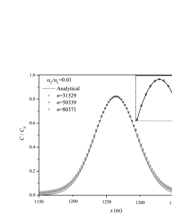
Figure 2: Concentration profiles at different spatial resolutions normalized to the initial concentration (symbols) as compared to the analytical solution given by Eq. (12) (solid line) after 300 days for $\alpha_{\rm T}/\alpha_{\rm L}=0.01$.

Figure 3: Concentration profiles at different spatial resolutions normalized to the initial concentration (symbols) as compared to the analytical solution given by Eq. (12) (solid line) after 300 days for $\alpha_{\rm T}/\alpha_{\rm L}=0.001$.

As the dispersivity increases from $\alpha_{\rm T}/\alpha_{\rm L}=0.1$ to 0.01 the deviation of the numerical profile from the analytical one increases. However, at the resolutions used here the differences in the RMSEs are small when doubling the number of particles, suggesting that at relatively high spatial resolutions the overall accuracy of the solution is almost independent of the dispersivity. As shown in Figs. 1, 2 and 3 convergence to the analytical solution is already obtained for 1,000,000 particles and 31,529 neighbours. When increasing the resolution to 2,000,000 particles and 50,339 neighbours the deviation between the numerical and analytical profiles is reduced by about $1.8\times 10^{-4}$% for $\alpha_{\rm T}/\alpha_{\rm L}=0.1$, and by $\sim 1.5\times 10^{-4}$% when passing from 2,000,000 particles and 31,529 neighbours to 4,000,000 particles and 80,371 neighbours. Similar percentages are obtained when increasing the resolution for $\alpha_{\rm T}/\alpha_{\rm L}=0.001$. In all cases, the major contribution to the error comes from the tail of the distribution when $C/C_{0}\to 0$, while it is minimum around the peak of the distribution where the concentration is maximum. This trends are consistent with the error bound in Eq. (6). If $h$ remains fixed, the SPH discretization errors drop for sufficiently large numbers of neighbours and the overall error is governed by the kernel approximation. This implies that consistency is being restored. On the other hand, accuracy demands that $h$ must decrease as $n$ increases in which case the numerical solution approaches the analytical one. This is in accordance with the scaling relations for which $h\sim n^{-0.247}$.

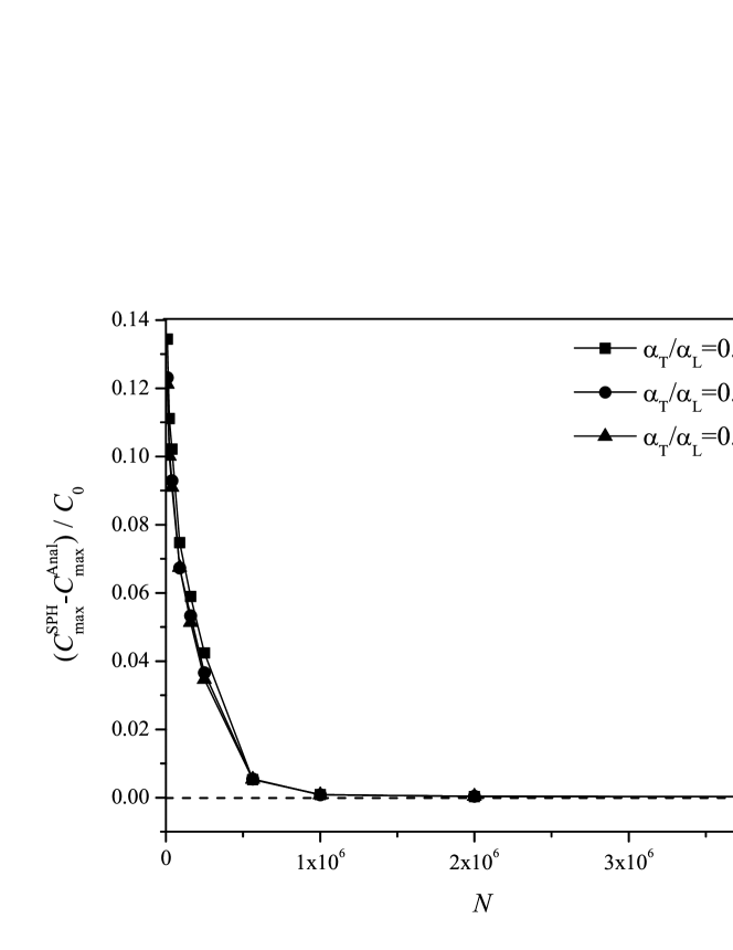
Figure 4: Difference between the SPH and exact value of the maximum concentration as a function of the total number of particles for the three dispersivity ratios considered. Convergence is clearly achieved for $N>1,000,000$ particles. The data for $N<1,000,000$ particles correspond to the previous simulations by Alvarado-Rodríguez et al. Alvarado2019 .

A drawback of any numerical method when dealing with the problem of anisotropic dispersion is the occurrence of negative concentrations away from the site of the solute Herrera2009 ; Herrera2013 ; Avesani2015 ; Alvarado2019 . Part of the problem lies on the tensor character of the dispersion coefficient given by Eq. (3). That is, when the off-diagonal components of the dispersion coefficient are nonzero, the solution is affected by artificial oscillations away from the maximum concentration, which then amplify nonlinearly. As shown in Figs. 1, 2 and 3, any small oscillation about the zero in the tail of the distribution (where $C/C_{0}\to 0$) can induce negative values of the concentration. This problem has posed severe limitations for the correct prediction of anisotropic solute dispersion and diffusion. As was pointed out by Compte and Metzler Compte1997 the problem is related to the nature of the classical Fick’s law given by Eq. (1), which due to its parabolic character is endowed with an infinite velocity of propagation. This can be seen from the analytical solution (12), where for any time a finite amount of diffusing contaminat will always be present at very large distances from the solute (i.e., in the tail of the concentration distribution), implying an infinitely fast propagation. While a solution to this problem goes through converting the Fick’s law into the hyperbolic Cattaneo’s equation Cattaneo1948

$$\tau\frac{d^{2}C}{dt^{2}}+\frac{dC}{dt}=\nabla\cdot(\mathbb{D}\cdot\nabla C)-C(\nabla\cdot{\bf v}),$$ (14)

where the term $\tau d^{2}C/dt^{2}$ is added ad hoc to force a finite propagation velocity along the transverse and longitudinal directions over a characteristic time constant $\tau$, here we explore the ability of the present scheme to suppress negative concentrations as the SPH consistency is restored by increasing the number of neighbours. Previous consistent SPH simulations by Alvarado-Rodríguez et al. Alvarado2019 have shown that convergence to the analytical solution with the present scheme is already attained for 1,000,000 particles and 31,529 neighbours, as shown in Fig. 4. It is evident from this figure that the difference between the SPH and the analytical solution tends to zero independently of the ratio $\alpha_{\rm T}/\alpha_{\rm L}$, meaning that full convergence is achieved when working with $N>1,000,000$ particles. However, this as not a sufficient condition to suppress the nonlinear amplification of small oscillations that are conducive to negative concentrations. In order to further explore under which conditions Eq. (1) can be used to model anomalous transport for large dispersivities with a consistent SPH scheme, we have increased the spatial resolution to 4,000,000 particles and 80,371 neighbours such that the ratio $n/N\approx 0.02$. In passing, we note that complete consistency will require $n/N\to 0$ for $N\to\infty$ and $n\to\infty$.

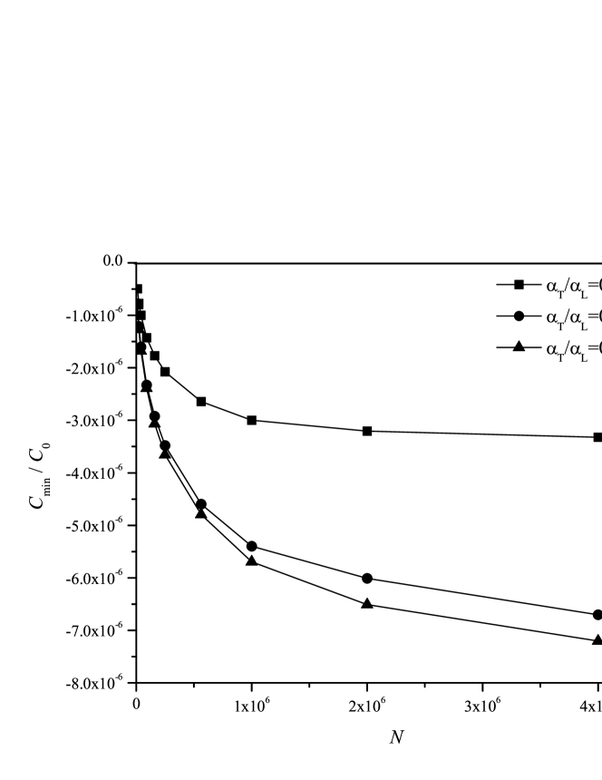
Figure 5: Magnitude of the maximum negative concentration values normalized to the initial concentration $C_{0}$ as a function of the total number of particles for all three dispersivity ratios. The data for $N<1,000,000$ particles correspond to the previous simulations by Alvarado-Rodríguez et al. Alvarado2019 .

Figure 5 displays the maximum values of the negative concentration as a function of the total number of particles for all three dispersivity ratios. As the resolution is increased, the magnitude of the negative values increases as a consequence of the decreased numerical diffusion which causes less damping of the unphysical oscillations. The smallest magnitudes occur for $\alpha_{\rm T}/\alpha_{\rm L}=0.1$. As the spatial resolution is increased, the rate of increase of the magnitude of the negative concentrations slows down. For $N>1,000,000$ the maximum negative concentration tends asymptotically to a constant value of $\approx-3.0\times 10^{-6}C_{0}$. At higher dispersivities the magnitude of the maximum negative concentration increases to $\approx-6.7\times 10^{-6}C_{0}$ (for $\alpha_{\rm T}/\alpha_{\rm L}=0.01$) and $\approx-7.2\times 10^{-6}C_{0}$ (for $\alpha_{\rm T}/\alpha_{\rm L}=0.001$), respectively, with $N=4,000,000$ particles. However, there is no much difference in the trend and values of the negative concentrations when the dispersivity is increased from $\alpha_{\rm T}/\alpha_{\rm L}=0.01$ to 0.001. Compared to $\alpha_{\rm T}/\alpha_{\rm L}=0.1$, a constant value of the maximum negative concentration with resolution will require using a much higher number of particles in these latter cases. Figures 6 depicts the concentration distributions at different times during the spreading of the contaminant plume for $\alpha_{\rm T}/\alpha_{\rm L}=0.1$ (left mosaic) and $\alpha_{\rm T}/\alpha_{\rm L}=0.001$ (right mosaic). The white bands along the transversal direction on both sides of the plume elongation represent the negative concentrations. These bands always appear in the tail of the distributions where the concentration decays asymptotically to zero.

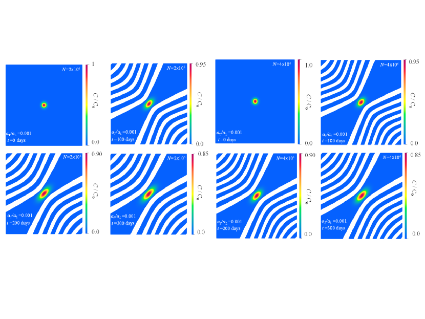
Figure 6: Distribution of the concentration normalized to the initial value $C_{0}$ at different times during the plume spreading for $\alpha_{\rm T}/\alpha_{\rm L}=0.001$. The left mosaic of frames corresponds to the run with 2,000,000 particles and 50,339 neighbours, while that on the right to the run with 4,000,000 particles and 80,371 neighbours. Negative concentrations are evidenced by the white bands along the transversal direction on both sides of the elongated plume.

Standard SPH simulations by Herrera and Beckie Herrera2013 for the same test case have produced maximum negative concentrations that are at least 4 orders of magnitude higher than those reported here. The MWSPH scheme proposed by Avesani et al. Avesani2015 , which is currently one of the best methods for the simulation of anisotropic dispersion and anomalous transport, produced absolute values of the negative concentrations less than about $10^{-7}C_{0}$ for $\alpha_{\rm T}/\alpha_{\rm L}=0.1$ and 0.01. In their case, the smoothing length of particle $a$ was defined according to the prescription $h_{a}=\sigma(m_{a}/\rho_{a})^{1/2}$ and the maximum absolute value of the negative concentrations was found to be sensitive to the value of $\sigma$ and the order $M$ of the Taylor series expansion of the concentration around the position $(x_{a},y_{a})$ of particle $a$, which was employed in the reconstruction procedure of the local concentration. For values of $M=3,4$ and $\sigma=3,2$, they reported magnitudes of the maximum negative concentrations of $10^{-12}-10^{-15}C_{0}$ for $\alpha_{\rm T}/\alpha_{\rm L}=0.1$ and $10^{-11}-10^{-13}C_{0}$ for $\alpha_{\rm T}/\alpha_{\rm L}=0.01$. On the other hand, according to Fig. 5 the almost constant behaviour of the $C_{\rm min}/C_{0}$-curve at high resolutions means that little can be improved by further increasing the resolution and the number of neighbours. That is, regardless of how much $N$ and $n$ are increased, the magnitude of the maximum negative concentrations will remain the same. According to Eq. (6), this suggests that for sufficiently large values of $n$ the global error will entirely depend on the kernel approximation through the last term in Eq. (6), which is $\propto h^{2}$. The sensitivity of the unphysical oscillations with the size of $h$ was further tested in an exploratory run with 4 million particles and using only 144 neighbours. This resulted in a smoothing length $h/L\approx 7.07\times 10^{-4}$ much smaller than those listed in Table 1. For such small value of $h$ the dominant term in Eq. (6) is the zeroth-order one given by $a_{0}/n$. Because of the excessive numerical diffusion carried by this term, the simulation resulted in a very blurry concentration field and was completely free of negative concentrations. The lesson to be learned from this result is that the occurrence of unphysical oscillations can be minimized if the consistency scaling relations are such that they provide smaller values of $h$ and correspondingly larger number of neighbours. This will introduce sufficient numerical diffusion through the term $a_{0}/n$ to guarantee damping of the oscillations, while maintaining reasonably good accuracy through small values of $h$. Unfortunately, the choice of the best scaling relation must be done by trial and error.

Figure 7: Time evolution of the relative difference between the SPH and analytical maximum concentration values for $\alpha_{\rm T}/\alpha_{\rm L}=0.1$ and varying spatial resolution. The box on the right indicate the spatial resolution for each curve in terms of the number of neighbours.

Figure 8: Time evolution of the relative difference between the SPH and analytical maximum concentration values for $\alpha_{\rm T}/\alpha_{\rm L}=0.001$ and varying spatial resolution. The box on the right indicate the spatial resolution for each curve in terms of the number of neighbours.

Figures 7 and 8 show the time variation of the relative difference between the analytical and numerical maximum concentrations for $\alpha_{\rm T}/\alpha_{\rm L}=0.1$ and 0.001, respectively. At early times, the relative differences are always less than $\sim 0.01$ for $\alpha_{\rm T}/\alpha_{\rm L}=0.1$ and $\sim 0.013$ for $\alpha_{\rm T}/\alpha_{\rm L}=0.001$ with $N=1,000,000$ particles. These differences drop to less than 0.4% for $\alpha_{\rm T}/\alpha_{\rm L}=0.1$ and 0.6% for $\alpha_{\rm T}/\alpha_{\rm L}=0.001$ at the highest resolution. The positivity of the differences implies that the SPH simulations are overestimating the maximum concentration. At $t=300$ days, the realtive error decays to less than 0.3% for the run with 4,000,000 particles regardless of the dispersivity. At early times, these differences are comparable to those reported by Avesani et al. Avesani2015 with their MWSPH scheme for $\alpha_{\rm T}/\alpha_{\rm L}=0.1$ and irregularly distributed particles. In their case, however, negative differences were obtained at later times when working with $\sigma=3$ and $M=4$. The results from both simulations agree that the shorter the smoothing length, the smaller the error at all times. However, according to Eq. (6) such level of accuracy must be accompanied by enough numerical diffusion to allow the unphysical oscillations to damp out in the course of the contaminant spreading.

5 Conclusions

We have presented highly resolved, consistent SPH simulations of anisotropic dispersion of a solute in a heterogeneous porous medium using as a framework the DualSPHysics code. First-order consistency is restored by working with large numbers of neighbours within the kernel support. The number of neighbours, $n$, and the smoothing length, $h$, are set in terms of the total number of particles according to the power-law relations $n\approx 2.81N^{0.675}$ and $h\approx 1.29n^{-0.247}$, which comply with the joint limit $N\to\infty$, $n\to\infty$ and $h\to 0$ for complete consistency Rasio2000 ; Zhu2015 ; Sigalotti2019 . The performance of the scheme is tested against the anisotropic spreading of a non-reactive, Gaussian solute plume that is instantaneously injected in a heterogeneous flow field for an irregularly distributed particles and dispersivity ratios of $\alpha_{\rm T}/\alpha_{\rm L}=0.1$, 0.01 and 0.001 Herrera2013 ; Avesani2015 ; Alvarado2019 , where $\alpha_{\rm L}$ and $\alpha_{\rm T}$ are the longitudinal and transverse dispersivities, respectively. As the number of particles and neighbours is increased to unprecedented values, i.e., $N=4,000,000$ and $n=80,371$, the distance between the numerical and analytical solutions is highly reduced with root-mean-square errors that are less than $4.5\times 10^{-4}$% in the worst case of high dispersivity ($\alpha_{\rm T}/\alpha_{\rm L}=0.001$).

The numerical solutions exhibit convergence rates comparable to those reported by Avesani et al. Avesani2015 with their highly accurate MWSPH scheme. However, in spite of the large number of neighbours used in the present simulations, the numerical solutions are not free of unphysical oscillations in the tail of the solute concentration distribution, which are reponsible for induction of negative concentrations. We find magnitudes of the maximum negative concentrations that are towards the upper limit of about $10^{-7}C_{0}$ reported by Avesani et al. Avesani2015 , where $C_{0}$ is the maximum initial concentration. The results suggest that the above scaling relations, which were chosen out of a family of infinite possible scalings to guarantee a sharp drop of the particle discretization errors while keeping reasonably large values of $h$ to alleviate the computational cost, was not enough to suppress the nonlinear growth of numerical oscillations in regions away from the contaminant plume, where the concentration tends asymptotically to zero. This is a consequence of the numerically dispersive nature of the simulation which introduces little numerical diffusion. An exploratory run with 4,000,000 particles and a low number of neighbours ($n=144$), which resulted in much smaller values of $h$ and much stronger diffusion due to the presence of irreducible zeroth-order discretization errors (because of the low number of neighbours), was free of negative concentrations away from the spreading plume, however, at the price of a very blurry concentration field everywhere due to the excessive numerical diffusion. Therefore, further consistent SPH simulations complying with the joint limit $N\to\infty$, $n\to\infty$ and $h\to 0$ must start working with scaling relations that guarantee a compromise between the number of neighbours and the size of $h$ such that sufficient numerical diffusion remains implicit in the scheme to damp out unphysical oscillations in regions where the concentration vanishes.

Conflict of interest

The authors declare that they have no conflict of interest.

References

- (1) Bear J (1988) Dynamics of fluids in porous media. Dover, New York
- (2) Le Potier C (2005) Finite volume monotone scheme for highly anisotropic diffusion operators on unstructured triangular meshes. Comptes Rendus Math 341(12):787–792. https://doi.org/10.1016/j.crma.2005.10.010
- (3) Nordbotten JM, Aavatsmark I (2005) Monotonicity conditions for control volume methods on uniform parallelogram grids in homogeneous media. Comput Geosci 9(1):61–72. https://doi.org/10.1007/s10596-005-5665-2
- (4) Mlacnik MJ, Durlofsky LJ (2006) Unstructured grid optimization for improved monotonicity of elliptic equations with highly anisotropic coefficients. J Comput Phys 216(1):337–361. https://doi.org/10.1016/j.jcp.2005.12.007
- (5) Yuan G, Sheng Z (2008) Monotone finite volume schemes for diffusion equations on polygonal meshes. J Comput Phys 227(12):6288–6312. https://doi.org/10.1016/j.jcp.2008.03.007
- (6) Lipnikov K, Svyatskiy D, Vassilevski Y (2009) Interpolation-free monotone finite volume method for diffusion equations on polygonal meshes. J Comput Phys 228(3):703–716. https://doi.org/10.1016/j.jcp.2009.09.031
- (7) Arbogast T, Huang C-S, Hung C-H (2012) A fully conservative Eulerian-Lagrangian stream-tube method for advection-diffusion problems. SIAM J Sci Comput 34(4):B447–B478. https://doi.org/10.1137/110840376
- (8) Kim M-Y, Wheeler MF (2014) Coupling discontinuous Galerkin discretizations using mortar finite elements for advection-diffusion-reaction problems. Comput Math Appl 67(1):181–198. https://doi.org/10.1016/j.camwa.2013.11.002
- (9) Beaudoin A, Huberson S, Rivoalen E (2003) Simulation of anisotropic diffusion by means of a diffusion velocity method. J Comput Phys 186(1):122–135. https://doi.org/10.1016/S0021-9991(03)00024-X
- (10) Herrera PA, Massabó M, Beckie RD (2009) A meshless method to simulate solute transport in heterogeneous porous media. Adv Water Resour 32(3):413–429. https://doi.org/10.1016/j.advwatres.2008.12.005
- (11) Herrera PA, Valocchi AJ, Beckie RD (2010) A multidimensional streamline-based method to simulate reactive solute transport in heterogeneous porous media. Adv Water Resour 33(7):711-727. https://doi.org/10.1016/j.advwatres.2010.03.001
- (12) Herrera PA, Beckie RD (2013) An assessment of particle methods for approximating anisotropic dispersion. Int J Numer Meth Fluids 71(5):634–651. https://doi.org/10.1002/fld.3676
- (13) Avesani D, Herrera P, Chiogna G, Bellin A, Dumbser M (2015) Smooth particle hydrodynamics with nonlinear moving-least-squares WENO reconstruction to model anisotropic dispersion in porous media. Adv Water Resour 80:43–59. https://doi.org/10.1016/j.advwatres.2015.03.007
- (14) Tran-Duc T, Bertevas E, Phan-Thien N, Khoo BC (2016) Simulation of anisotropic diffusion processes in fluids with smoothed particle hydrodynamics. Int J Numer Meth Fluids 82:730–747. https://doi.org/10.1002/fld.4238
- (15) Monaghan JJ (1992) Smoothed particle hydrodynamics. Annu Rev Astron Astrophys 30:543–574. https://doi.org/10.1146/annurev.aa.30.090192.002551
- (16) Liu GR, Liu MB (2003) Smoothed particle hydrodynamics: A meshfree particle method. World Scientific, Singapore
- (17) Boso F, Bellin A, Dumbser M (2013) Numerical simulations of solute transport in highly heterogeneous formations: A comparison of alternative numerical schemes. Adv Water Resour 52:178–189. https://doi.org/10.1016/j.advwatres.2012.08.006
- (18) Alvarado-Rodríguez CE, Sigalotti L Di G, Klapp J (2019) Anisotropic dispersion with a consistent smoothed particle hydrodynamics scheme. Adv Water Resour 131:103374. https://doi.org/10.1016/j.advwatres.2019.07.004
- (19) Rasio FA (2000) Particle methods in astrophysical fluid dynamics. Prog Theoret Phys Suppl 138:609–621. https://doi.org/10.1143/PTPS.138.609
- (20) Read JI, Hayfield T, Agertz O (2010) Resolving mixing in smoothed particle hydrodynamics. Mon Not R Astron Soc 405(3):1513–1530. https://doi.org/10.1111/j.1365-2966.2010.16577.x
- (21) Zhu Q, Hernquist L, Li Y (2015) Numerical convergence in smoothed particle hydrodynamics. Astrophys J 800:6. https://doi.org/10.1088/0004-637X/800/1/6
- (22) Sigalotti L Di G, Klapp J, Rendón O, Vargas CA, Peña-Polo F (2016) On the kernel and particle consistency in smoothed particle hydrodynamics. Appl Numer Math 108:242–255. http://dx.doi.org/10.1016/j.apnum.2016.05.007
- (23) Sigalotti L Di G, Rendón O, Klapp J, Vargas CA, Cruz F (2019) A new insight into the consistency of the SPH interpolation formula. Appl Math Comput 356:50–73. https://doi.org/10.1016/j.amc.2019.03.018
- (24) Wendland H (1995) Piecewise polynomial, positive definite and compactly supported radial functions of minimal degree. Adv Comput Math 4(1):389–396. https://doi.org/10.1007/BF02123482
- (25) Dehnen W, Aly H (2012) Improving convergence in smoothed particle hydrodynamics without pairing instability. Mon Not R Astron Soc 425(2):1068–1082. https://doi.org/10.1111/j.1365-2966.2012.21439.x
- (26) Gómez-Gesteira M, Rogers BD, Crespo AJC, Dalrymple RA, Narayanaswamy M, Domínguez JM (2012) SPHysics – development of a free-surface fluid solver – Part 1: Theory and formulations. Comput Geosci 48:289–299. https://doi.org/10.1016/j.cageo.2012.02.029
- (27) Crespo AJC, Domínguez JM, Rogers BD, Gómez-Gesteira M, Longshaw S, Canelas R, Vacondio R, Barreiro A, García-Feal O (2015) DualSPHysics: Open-source parallel CFD solver based on smoothed particle hydrodynamics (SPH). Comput Phys Commun 187:204–216. https://doi.org/10.1016/j.cpc.2014.10.004
- (28) Compte, A, Metzler, R (1997) The generalized Cattaneo equation for the description of anomalous transport processes. J Phys A 30(21):7277–7289. https://doi.org/10.1088/0305-4470/30/21/006
- (29) Cattaneo, C (1948) Sulla conduzione del calore. Atti Semin Mat Fis Univ Modena e Reggio Emilia 3:83–101.