A determination of the longitudinal structure function $F_{L}$ from the parametrization of $F_{2}$ based on the Laplace transformation

Abstract

I calculate the longitudinal structure function, using Laplace transform techniques, from the parametrization of the structure function $F_{2}(x,Q^{2})$ and its derivative at low values of the Bjorken variable $x$. I consider the effect of the charm quark mass to the longitudinal structure function, which leads to rescaling variable for $n_{f}=4$. The results are compared with the H1 collaboration data and the CTEQ-Jefferson Lab (CJ) collaboration [Phys.Rev.D 93, 114017 (2016)] parametrization model. The obtained results with the Bjorken variable of $x$ are found to be comparable with the results L.P.Kaptari et al. [Phys.Rev.D 99, 096019 (2019)] which is based on the Mellin transform techniques.

.1 Introduction

Understanding the basic internal structure of nucleon and the quest for the ultimate constituents has always been important in high energy physics. In ultra-high energy processes, at extremely high inelasticity $y$, the longitudinal structure function becomes predominant and its behavior will be extended down to very low $x$ in the Large Hadron electron Collider (LHeC). The Large Hadron Electron Collider (LHeC), a possible future upgrade of the LHC, will extend the HERA DIS measurement into a much smaller region of $x$ and larger region of $Q^{2}$. In this region the longitudinal structure function becomes predominant. In the LHeC design report [1], a simulation study at low $x$ for the longitudinal structure function has been performed in considerable detail. This has recently been updated [2], with still enlarged luminosity and improved detector systematics. The $F_{L}$ measurements with the LHeC will reach a precision of a few percent. They are considered to be extended down to $x$ below $10^{-6}$ with the the Future Circular Collider electron- hadron (FCC-eh). In the future, the electron-proton colliders will generate even more data with lower $x$ values and high values of $Q^{2}$. The longitudinal structure function is directly related to the gluon distribution in the proton and its behavior has been predicted by Altarelli and Martinelli [3] equation. Indeed, this represents a crucial test on the validity of the perturbative QCD (pQCD) framework at small $x$, when compared the experimental data with theoretical predictions.
The recent articles in Ref.[4] by Kaptari $et~{}al$. revives the parametrization of the longitudinal structure function by using the parametrization of the structure function $F_{2}$. The parametrization of the proton structure function [5] is a fit to HERA data on deep-inelastic lepton-nucleon scattering (DIS) at low $x$ in a wide range of the momentum transfer $Q^{2}$, $(1~{}\mathrm{GeV}^{2}<Q^{2}<3000~{}\mathrm{GeV}^{2})$. This fit describes fairly well the available experimental data on the reduced cross sections, at asymptotically low $x$, and provides the parametrization of the structure function $F_{2}$ which is relevant in investigations of ultra-high energy processes. This parametrization [5] provides reliable structure function $F_{2}$ by the following form

$$F_{2}(x,Q^{2}) = D(Q^{2})(1-x)^{n}\sum_{m=0}^{2}A_{m}(Q^{2})L^{m},$$ (1)

where the explicit expression for the proton structure function and effective parameters are defined in Appendix A and Table I. The authors of Ref.[4] show that the longitudinal structure function in the leading-order (LO) approximation is considered in the same form of the parametrization of the structure function $F_{2}$ (i.e., Eq.(1)), which is

$$F_{L}(x,Q^{2}) = (1-x)^{\nu}\sum_{m=0}^{2}C_{m}(Q^{2})L^{m}.$$ (2)

The parametrization of structure functions (i.e., Eqs.(1) and (2)), suggested in Refs.[4] and [5], are in a full accordance with the Froissart predictions. In this paper I introduce a method to calculate $F_{L}(x,Q^{2})$ inside the proton by using the Laplace transform techniques. Several methods to relate $F_{L}$ and $F_{2}$ scaling violation to the gluon density at small $x$ were suggested previously [6-12]. To study the longitudinal structure function I use the Laplace-transform technique for solving the Altarelli- Martinelli equation by employing the parametrization of the structure function $F_{2}$.

.2 Method

In $s$-space the obtained equations [13-18] for the structure functions, which relate both the quark and gluon densities, defined by the following forms as

$$\frac{\partial{f_{2}(s,Q^{2})}}{\partial{\ln}Q^{2}} = \Phi_{f}(s)f_{2}(s,Q^{2})+<e^{2}>\Theta_{f}(s)g(s,Q^{2}),$$

$$f_{L}(s,Q^{2}) = \Phi_{L}(s)f_{2}(s,Q^{2})+<e^{2}>\Theta_{L}(s)g(s,Q^{2}).$$

The Laplace-transform of the distribution functions read

$${\mathcal{L}}[\mathcal{\widehat{F}}_{L}(\upsilon,Q^{2});s] = f_{L}(s,Q^{2}),$$

$${\mathcal{L}}[\mathcal{\widehat{F}}_{2}(\upsilon,Q^{2});s] = f_{2}(s,Q^{2})$$ (4)

where

$$\mathcal{\widehat{F}}_{L}(\upsilon,Q^{2}) = \frac{4\pi}{\alpha_{s}(Q^{2})}F_{L}(e^{-\nu},Q^{2}),$$

$$\frac{\partial{\mathcal{\widehat{F}}_{2}(\upsilon,Q^{2})}}{\partial{\ln}Q^{2}} = \frac{4\pi}{\alpha_{s}(Q^{2})}\frac{{\partial}F_{2}(e^{-\nu},Q^{2})}{\partial{\ln}Q^{2}}.$$ (5)

The $\nu$ variable is $\nu{\equiv}\ln(1/x)$ and $<e^{2}>$ is the average of the charge $e^{2}$ for the active quark flavors, $<e^{2}>=n_{f}^{-1}\sum_{i=1}^{n_{f}}e_{i}^{2}$. It should be noted that the Laplace transform of convolution factors is simply the ordinary product of the Laplace transform of the factors.
The coefficient functions $\Phi$ and $\Theta$ in $s$-space are given by

$$\Phi_{L}(s) = 4C_{F}\frac{1}{2+s},$$

$$\Theta_{L}(s) = 8n_{f}(\frac{1}{2+s}-\frac{1}{3+s}),$$

$$\Theta_{f}(s) = 2n_{f}(\frac{1}{1+s}-\frac{2}{2+s}+\frac{2}{3+s}),$$

$$\Phi_{f}(s) = 4-\frac{8}{3}(\frac{1}{1+s}+\frac{1}{2+s}+2(\psi(s+1)+\gamma_{E})),$$

where $\psi(x)$ is the digamma function and $\gamma_{E}=0.5772156..$ is Euler constant. For the SU(N) gauge group, $C_{F}=4/3$ is the color Cassimir operator in QCD. In the above equations, $\psi(s)$ is defined by $\psi(s)=\frac{d}{ds}{\ln}\Gamma(s)$ and $S(s)=\psi(s+1)-\psi(1)$ expressed [4] by $S(s)=-{\ln}2-\sum_{l=0}^{\infty}\frac{(-1)^{l+1}}{s+l+1}$.
Eventually, the longitudinal structure function is defined into the proton structure function and the derivative of the proton structure function with respect to $\ln{Q^{2}}$ in $s$-space by the following form

$$f_{L}(s,Q^{2})=\frac{\alpha_{s}(Q^{2})}{4\pi}k(s)f_{2}(s,Q^{2})+h(s)\frac{\partial{f_{2}(s,Q^{2})}}{\partial{\ln}Q^{2}},$$ (7)

where $k(s)=\Phi_{L}(s)-\frac{\Theta_{L}(s)}{\Theta_{f}(s)}\Phi_{f}(s)$ and $h(s)=\frac{\Theta_{L}(s)}{\Theta_{f}(s)}$. The inverse Laplace transform of $k(s)$ and $h(s)$ is given by the kernels $\widehat{\eta}(\nu){\equiv}{\mathcal{L}}^{-1}[k(s);\nu]$ and $\widehat{J}(\nu){\equiv}{\mathcal{L}}^{-1}[h(s);\nu]$ respectively. Therefore the solution of the inverse Laplace transform of coefficients $k(s)$ and $h(s)$ can be converted to $\nu$-space as

$$\widehat{\eta}(\nu) = \frac{32}{3}e^{(-2\nu)}+e^{-\frac{3}{2}\nu}[\frac{64}{21}\sqrt{7}(\ln(2)+3)\sin(\frac{1}{2}\sqrt{7}\nu)$$ (8)

$$-\frac{64}{3}(\ln(2)+1)\cos(\frac{1}{2}\sqrt{7}\nu)],$$

and

$$\widehat{J}(\nu)=e^{-\frac{3}{2}\nu}[4\cos(\frac{1}{2}\sqrt{7}\nu)-\frac{4}{7}\sqrt{7}\sin(\frac{1}{2}\sqrt{7}\nu)].$$ (9)

Consequently, the general relation between the structure functions in $x$-space is given by

$$F_{L}(x,Q^{2}) = \frac{\alpha_{s}(Q^{2})}{4\pi}\int_{x}^{1}F_{2}(y,Q^{2})\eta(\frac{x}{y})\frac{dy}{y}$$ (10)

$$+\int_{x}^{1}\frac{{\partial}F_{2}(y,Q^{2})}{\partial{\ln}Q^{2}}J(\frac{x}{y})\frac{dy}{y},$$

where

$$\frac{{\partial}F_{2}(x,Q^{2})}{\partial{\ln}Q^{2}} = F_{2}(x,Q^{2})[\frac{{\partial}{\ln}D(Q^{2})}{\partial{\ln}Q^{2}}$$

$$+\frac{{\partial}{\ln}\sum_{m=0}^{2}A_{m}(Q^{2})L^{m}}{\partial{\ln}Q^{2}}],$$

and

$$\eta(\frac{x}{y}) = \frac{32}{3}(\frac{x}{y})^{2}+(\frac{x}{y})^{3/2}[\frac{64}{21}\sqrt{7}(\ln(2)+3)\sin(\frac{1}{2}\sqrt{7}{\ln}(\frac{y}{x}))$$

$$-\frac{64}{3}(\ln(2)+1)\cos(\frac{1}{2}\sqrt{7}{\ln}(\frac{y}{x}))],$$

$$J(\frac{x}{y}) = (\frac{x}{y})^{3/2}[4\cos(\frac{1}{2}\sqrt{7}{\ln}(\frac{y}{x}))-\frac{4}{7}\sqrt{7}\sin(\frac{1}{2}\sqrt{7}{\ln}(\frac{y}{x}))].$$

Therefore the longitudinal structure function due to the Laplace-transform method is obtained by the parametrization of the structure function $F_{2}$ and its derivative ${{\partial}F_{2}(x,Q^{2})}/{\partial{\ln}Q^{2}}$. In order to make the effect of production threshold for charm quark, I use the rescaling variable $\chi$ which introduced by Aivazis, Collins, Olness and Tung (ACOT) in Ref.[19]. Therefore, the longitudinal structure function is defined by the rescaling variable $\chi$ where $\chi=x(1+\frac{4m_{c}^{2}}{Q^{2}})$. The rescaling variable $\chi$ at high $Q^{2}$ values ($m_{c}^{2}/Q^{2}{\ll}1$) reduces to the Bjorken variable $x$ as $\chi{\rightarrow}x$ [19]. The running charm mass is obtained as $m_{c}=1.29^{+0.077}_{-0.053}\mathrm{GeV}$, where the uncertainties are obtained through adding the experimental fit, model and parametrization uncertainties in quadrature [20,21].

.3 Results and Discussion

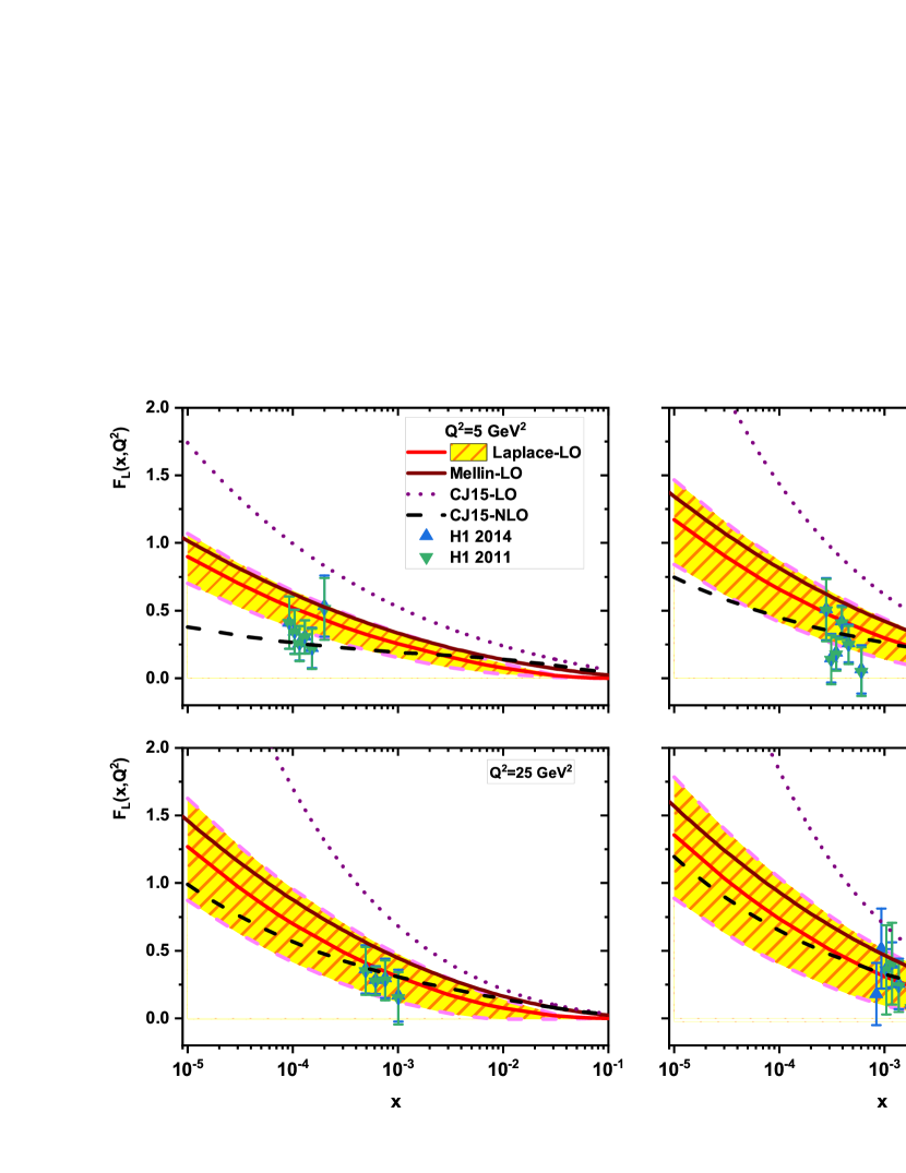
In Ref.[4] the QCD parameter $\Lambda$ has been extracted due to $\alpha_{s}(M_{z}^{2})=0.1166$, which for four number of active flavor is defined by $\Lambda=136.8~{}\mathrm{MeV}$. With the explicit form of the proton structure function, I can proceed to extract the longitudinal structure function $F_{L}(x,Q^{2})$ from data mediated by the parametrization of the structure function $F_{2}(x,Q^{2})$ and its derivative. I have calculated the $x$-dependence of the longitudinal structure function at several fixed values of $Q^{2}$ corresponding to H1 collaboration data [21,22]. Results are presented and compared with H1 collaboration data [21,22] and the parametrization of the longitudinal structure function $F_{L}(x,Q^{2})$ [3] at leading-order approximation in Fig.1. The error bands illustrated in this figure are into the charm-quark mass uncertainty and the statistical errors in the parametrization of $F_{2}(x,Q^{2})$, where the fit parameter errors are shown in Table I. It is seen that, for all values of the presented $Q^{2}$ with respect to the rescaling variable, the extracted longitudinal structure function due to the Laplace transform method is comparable with the H1 collaboration data. In order to present more detailed discussions on our findings, the results for the longitudinal structure function compared with leading and next-to-leading order (LO and NLO respectively) of CJ15 [23] in this figure. Also the obtained longitudinal structure functions compared with the Mellin transforms method [4] at leading order approximation in Fig.1.
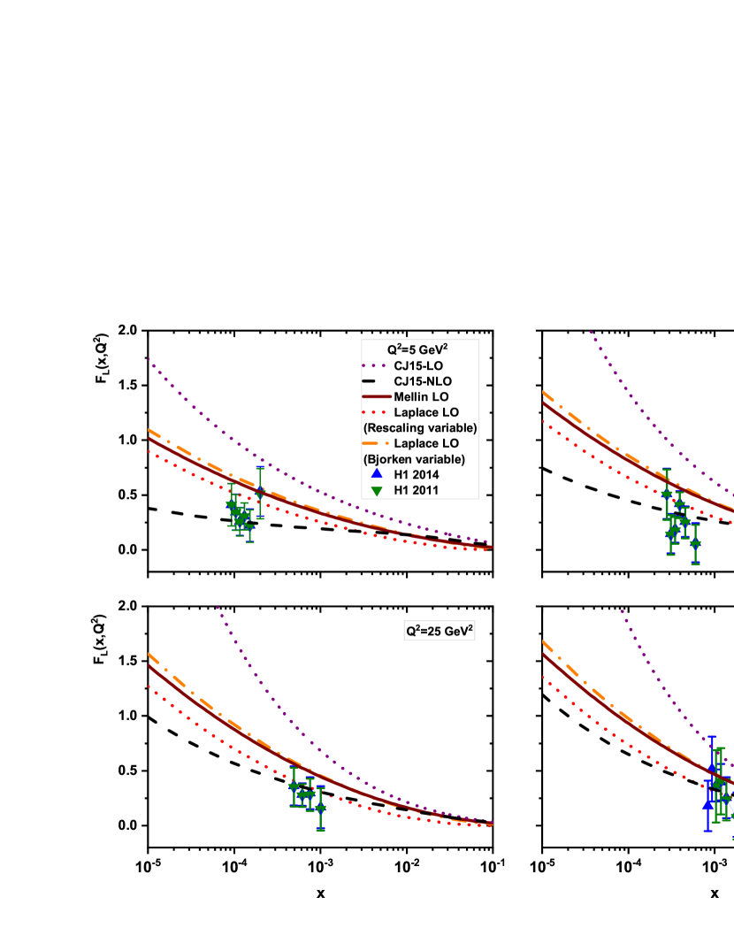
The effect of the charm quark mass in the splitting functions into the rescaling variable is considered in Fig.2. These results (with the rescaling and Bjorken variables) in Fig.2 compared with CJ15 at LO and NLO approximations and H1 collaboration data. As can be seen in Fig.2, the results with Bjorken variable are comparable with the results in Ref.[4] which is based on the Mellin transforms method. Indeed, the Mellin and Laplace transform methods have the same behavior with two difference schemes. These results compared with the obtained longitudinal structure functions with respect to the rescaling variable. Indeed, the rescaling variable improves the longitudinal structure functions in comparison with the Mellin transform that is based on the Bjorken variable when the longitudinal structure functions compared with H1 collaboration data.
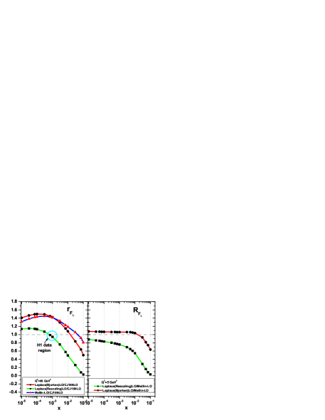
The accuracy of the Laplace and Mellin transform methods at LO approximation in comparison with the NLO CJ15 [23] is illustrated in Fig.3 by the ratio

$$r_{F_{L}} = \frac{F_{L}^{\mathrm{Analytic}}(x,Q^{2})}{F_{L}^{\mathrm{CJ15NLO}}(x,Q^{2})},$$

where analytic return to the Laplace transforms method at LO approximation by the Bjorken and rescaling variables and also the Mellin transforms method at LO approximation by the Bjorken variable. In the left-hand column of Fig.3, I show the fractional accuracy $r_{F_{L}}$ for Laplace and Mellin transforms methods due to the Bjorken and rescaling variables in comparison with the NLO CJ15 at $Q^{2}=45~{}\mathrm{GeV}^{2}$. Fig.3 shows that the longitudinal structure functions obtained at LO approximation by Laplace transforms method from the rescaling variable are consistent with the H1 collaboration data at $Q^{2}=45~{}\mathrm{GeV}^{2}$ and can be extended to all $Q^{2}$ values. Both the Laplace and Mellin transforms method at LO approximation by the Bjorken variable are not agreement with the H1 data region in the domain $x{\simeq}10^{-3}$. Also, in the right-hand column of Fig.3, the fractional accuracy $R_{F_{L}}$ at $Q^{2}=5~{}\mathrm{GeV}^{2}$ for Laplace transforms method due to the Bjorken and rescaling variables in comparison with the Mellin transforms method at LO approximation by the Bjorken scaling is shown by the following form

$$R_{F_{L}} = \frac{F_{L}^{\mathrm{Laplace}}(x,Q^{2})}{F_{L}^{\mathrm{Mellin}}(x,Q^{2})}.$$

This figure shows that $R_{F_{L}}$ for Bjorken scaling is essentially constant and approximately equal to one for all $x{\lesssim}0.01$. The discrepancies between the Laplace and Mellin by the Bjorken scaling are small, but they are large when the rescaling variable is considered. Indeed these results due to the rescaling variable are comparable with the CJ15 NLO and H1 collaboration data in H1 data domain.
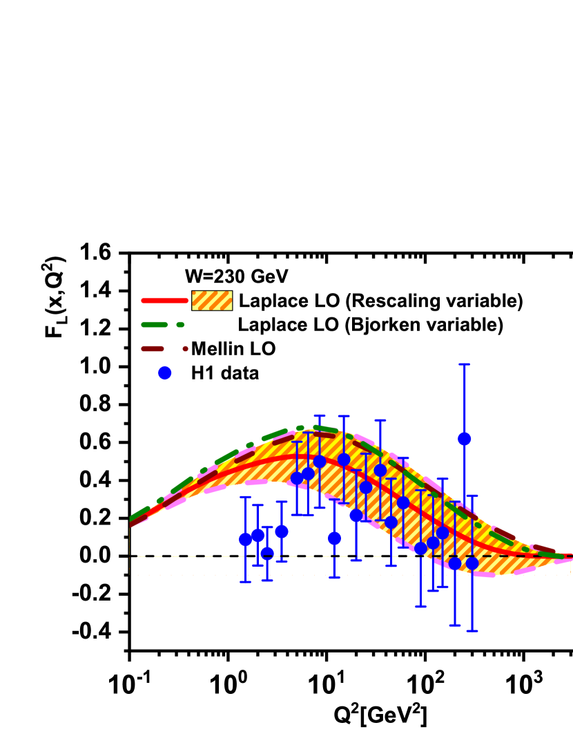
In Fig.4, I show the $Q^{2}$-dependence of the longitudinal structure function at low $x$. Results of calculations and comparison with the H1 collaboration data [21,22] are presented in this figure (i.e., Fig.4), where the charm quark mass effects is considered in the rescaling variable. These results have been performed at fixed value of the invariant mass $W$ as $W=230~{}\mathrm{GeV}$. Figure 4 shows that the parametrization of parton distributions provides correct behaviors of the extracted $F_{L}(x,Q^{2})$ in comparison with the Mellin transforms method. Over a wide range of variable $Q^{2}$, the extracted longitudinal structure functions are in a good agreement with experimental data in comparison with the parametrization of the longitudinal structure function $F_{L}(x,Q^{2})$ at leading-order approximation. At low values of $Q^{2}$, the extracted results are still above the experimental data. The error bands illustrated in this figure are into the charm-quark mass uncertainty and the statistical errors in the parametrization of the structure function $F_{2}(x,Q^{2})$, where the fit parameter errors are shown in Table I.
Also comparison between the longitudinal structure functions, into the rescaling and Bjorken scaling variables, are shown in Fig.4 for a wide range of $Q^{2}$. These results (with the rescaling and Bjorken variables) in Fig.4 compared with the H1 collaboration data [21]. As can be seen in this figure, the Laplace and Mellin transform methods in the Bjorken scaling are comparable together in a wide range of $Q^{2}$ values at fixed center-of-mass energy. At fixed value of the invariant mass $W=230~{}\mathrm{GeV}$, the rescaling variable improve the longitudinal structure function results in comparable with the H1 collaboration data.

In conclusion, I have presented a certain theoretical model to describe the longitudinal structure function based on the Laplace transform method at low values of $x$. A detailed analysis has been performed to find an analytical solution of the longitudinal structure function from the parametrization of the structure function $F_{2}(x,Q^{2})$ and its derivative. The effect of massive quarks in the splitting functions is considered into the rescaling variable. The calculations are consistent with the H1 collaboration data from HERA collider. As a next step, I plan to take into account the high-order corrections in a similar manner as in Ref. [4] (Phys.Rev.D 99, 096019 (2019)) since these corrections are important in the region of small $Q^{2}$, also the non-linear corrections improve the longitudinal structure function behavior at low $Q^{2}$.

.4 ACKNOWLEDGMENTS

The author is thankful to the Razi University for financial support of this project.

.5 Appendix A

The proton structure function parameterized in Ref.[5] provide good fits to the HERA data at low $x$ and large $Q^{2}$ values. The explicit expression for the proton structure function, with respect to the Block-Halzen fit, in a range of the kinematical variables $x$ and $Q^{2}$, $x{\leq}0.1$ and $0.15~{}\mathrm{GeV}^{2}<Q^{2}<3000~{}\mathrm{GeV}^{2}$, is defined by the following form

$$F^{\gamma p}_{2}(x,Q^{2}) = D(Q^{2})(1-x)^{n}[C(Q^{2})+A(Q^{2})\ln(\frac{1}{x}\frac{Q^{2}}{Q^{2}+\mu^{2}})$$ (11)

$$+B(Q^{2})\ln^{2}(\frac{1}{x}\frac{Q^{2}}{Q^{2}+\mu^{2}})],$$

where

$$A(Q^{2}) = a_{0}+a_{1}{\ln}(1+\frac{Q^{2}}{\mu^{2}})+a_{2}{\ln}^{2}(1+\frac{Q^{2}}{\mu^{2}}),$$

$$B(Q^{2}) = b_{0}+b_{1}{\ln}(1+\frac{Q^{2}}{\mu^{2}})+b_{2}{\ln}^{2}(1+\frac{Q^{2}}{\mu^{2}}),$$

$$C(Q^{2}) = c_{0}+c_{1}{\ln}(1+\frac{Q^{2}}{\mu^{2}}),$$

$$D(Q^{2}) = \frac{Q^{2}(Q^{2}+\lambda M^{2})}{(Q^{2}+M^{2})^{2}}.$$ (12)

Here $M$ is the effective mass and $\mu^{2}$ is a scale factor. The additional parameters with their statistical errors are given in Table I.

Table 1: The effective parameters at low $x$ for $0.15~{}\mathrm{GeV}^{2}<Q^{2}<3000~{}\mathrm{GeV}^{2}$ provided by the following values. The fixed parameters are defined by the Block-Halzen fit to the real photon-proton cross section as $M^{2}=0.753\pm 0.068~{}\mathrm{GeV}^{2}$, $\mu^{2}=2.82\pm 0.290~{}\mathrm{GeV}^{2}$ and $c_{0}=0.255\pm 0.016$ [5].

parameters                    value
$a_{0}$	$8.205\times 10^{-4}~{}~{}\pm 4.62\times 10^{-4}$
$a_{1}$	$-5.148\times 10^{-2}\pm 8.19\times 10^{-3}$
$a_{2}$	$-4.725\times 10^{-3}\pm 1.01\times 10^{-3}$
$b_{0}$	$2.217\times 10^{-3}\pm 1.42\times 10^{-4}$
$b_{1}$	$1.244\times 10^{-2}\pm 8.56\times 10^{-4}$
$b_{2}$	$5.958\times 10^{-4}\pm 2.32\times 10^{-4}$
$c_{1}$	$1.475\times 10^{-1}~{}\pm 3.025\times 10^{-2}$
$n$	$11.49\pm 0.99$
$\lambda$	$2.430~{}\pm 0.153$
$\chi^{2}(\mathrm{goodness~{}of~{}fit})$	$0.95$

I References

1. J.Abelleira Fernandez et al., [LHeC Collaboration], J.Phys.G39, 075001(2012).
2. P. Agostini et al. (LHeC Collab- oration and FCC-he Study Group), CERN-ACC-Note- 2020-0002, arXiv:2007.14491 [hep-ex] (2020).
3. G.Altarelli and G.Martinelli, Phys.Lett.B76, 89(1978).
4. L.P.Kaptari et al., Phys.Rev.D 99, 096019 (2019); JETP Lett.109, 281(2019).
5. M. M. Block, L. Durand and P. Ha, Phys. Rev. D 89, 094027 (2014).
6. G.R.Boroun, JETP lett.114, 3(2021); Eur.Phys.J.Plus 135, 68(2020); Phys.Rev.C 97, 015206(2018); Eur.Phys.J.Plus 129, 19(2014).
7. J.Blumlein, J.Phys.G 19, 1623 (1993); A.M.Cooper-Sarkar, Z.Phys.C 39, 281 (1988); J.Schwartz, arXiv [hep-ex]:1010.1023 (2010); S.Simula, Phys.Lett.B 574, 189(2003).
8. B.Rezaei and G.R.Boroun, Eur.Phys.J.A 56, 262(2020).
9. N.Baruah, M.K.Das and J.K.Sarma, Eur.Phys.J.Plus 129, 229 (2014).
10. G.R.Boroun, B.Rezaei and J.K.Sarma, Int.J.Mod.Phys.A 29, 1450189 (2014).
11. A.V.Kotikov, A.V.Lipatov and N.P.Zotov, J.Exp.Theo.Phys. 101, 811 (2005); Eur.Phys.J.C 27, 219(2003); A.V.Kotikov and G.Parente, Mod.Phys.Lett.A 12, 963 (1997); A.V.Kotikov, J.Exp.Theo.Phys. 80, 979 (1995).
12. G.R.Boroun and B.Rezaei, Eur.Phys.J.C 72, 2221 (2012); Phys.Lett.B 816, 136274 (2021).
13. M.M.Block, L.Durand, P.Ha and D.W.Mckay, Phys.Rev.D 83, 054009 (2011).
14. G.R.Boroun, S.Zarrin and F.Teimoury, Eur.Phys.J.Plus 130, 214 (2015).
15. H.Khanpour, A.Mirjalili and S.Atashbar Tehrani, Phys.Rev.C 95, 035201 (2017).
16. G.R.Boroun and B.Rezaei, Eur.Phys.J.C 73, 2412 (2013).
17. S.M.Moosavi Nejad, H.Khanpour, S.Atashbar Tehrani and M.Mahdavi, Phys.Rev.C 94, 045201 (2016).
18. S.Dadfar and S.Zarrin, Eur.Phys.J.C 80, 319 (2020).
19. M.A.G.Aivazis et al., Phys.Rev.D 50, 3102 (1994).
20. H1 and ZEUS Collaborations (Abramowicz H. et al.), Eur. Phys. J. C 78, 473 (2018).
21. H1 Collab. (V.Andreev , A.Baghdasaryan, S.Baghdasaryan et al.), Eur.Phys.J.C74, 2814(2014).
22. H1 Collab. (F.D.Aaron , C.Alexa, V.Andreev et al.),Eur.Phys.J.C71, 1579 (2011).
23. A.Accardi, L.T.Brady, W.Melnitchouk, J.F.Owens, N.Sato, Phys.Rev.D 93, 114017 (2016).

Figure 1: The longitudinal structure function, based on the rescaling variable by the Laplace transform method, extracted in comparison with the H1 experimental data (up-triangle H1 2014, down-triangle H1 2011) [21,22] as accompanied with total errors. The error bands are due to the charm-quark mass uncertainty and the statistical errors in the parametrization of $F_{2}(x,Q^{2})$ and its derivative. The dashed, dot and solid lines represent the CJ15 at NLO and LO approximations [23] and the Mellin transforms method [4] at the LO approximation respectively.

Figure 2: The longitudinal structure functions based on the rescaling (dot lines) and Bjorken (dashed-dot lines) variables compared with the H1 experimental data (up-triangle H1 2014, down-triangle H1 2011) [21,22] as accompanied with total errors, the CJ15 at NLO and LO approximations [23] (dashed and dot lines) and the Mellin transform method [4] (solid lines) at LO approximation respectively.

Figure 3: Left-hand column: comparison of the $r_{F_{L}}$ obtained by the Laplace and Mellin transforms methods by the Bjorken and rescaling variables with CJ15 NLO at $Q^{2}=45~{}\mathrm{GeV}^{2}$. Right-hand column: comparison of the $R_{F_{L}}$ obtained by the Laplace transforms method by the Bjorken and rescaling variables with and the Mellin transforms method at $Q^{2}=5~{}\mathrm{GeV}^{2}$.

Figure 4: $Q^{2}$ dependence of the extracted longitudinal structure function at fixed value of the invariant mass $W=230~{}\mathrm{GeV}$, into the rescaling (solid curve) and Bjorken (dashed-dot curve) variables compared with the Mellin transform method [4](dashed curve) at the LO approximation. The error bands are due to the charm-quark mass uncertainty and the statistical errors in the parametrization of $F_{2}(x,Q^{2})$ and its derivative. Experimental data by the H1 Collaboration are taken from Ref. [21] as accompanied with total errors.