Fairness-Aware Online Meta-learning

Abstract.

In contrast to offline working fashions, two research paradigms are devised for online learning: (1) Online Meta Learning (OML) (Finn et al., 2019; Yao et al., 2020; Nagabandi et al., 2019) learns good priors over model parameters (or learning to learn) in a sequential setting where tasks are revealed one after another. Although it provides a sub-linear regret bound, such techniques completely ignore the importance of learning with fairness which is a significant hallmark of human intelligence. (2) Online Fairness-Aware Learning (Bechavod et al., 2019; Gillen et al., 2018; Patil et al., 2020). This setting captures many classification problems for which fairness is a concern. But it aims to attain zero-shot generalization without any task-specific adaptation. This therefore limits the capability of a model to adapt onto newly arrived data. To overcome such issues and bridge the gap, in this paper for the first time we proposed a novel online meta-learning algorithm, namely FFML, which is under the setting of unfairness prevention. The key part of FFML is to learn good priors of an online fair classification model’s primal and dual parameters that are associated with the model’s accuracy and fairness, respectively. The problem is formulated in the form of a bi-level convex-concave optimization. Theoretic analysis provides sub-linear upper bounds $O(\log T)$ for loss regret and $O(\sqrt{T\log T})$ for violation of cumulative fairness constraints. Our experiments demonstrate the versatility of FFML by applying it to classification on three real-world datasets and show substantial improvements over the best prior work on the tradeoff between fairness and classification accuracy.

1. Introduction

It’s no secret that bias is present everywhere in our society, such as recruitment, loan qualification, recidivism, etc. The manifestation of bias can be often as fraught as race or gender. Because of this, machine learning algorithms have several examples of training models, many of which have received strong criticism for exhibiting unfair bias. Critics have voiced that human bias potentially has an influence on nowadays technology, which leads to outcomes with unfairness.

With biased input, the main goal of training an unbiased model in machine learning is to make the output fair. Group-fairness, also known as statistic parity, ensures the equality of a predictive utility across different sub-populations. In other words, the predictions are statistically independent on protected variables, e.g., race or gender. In the real world, data with bias are likely available only sequentially and also from a non-stationary task distribution. For example, a recent news (Miller, 2020) by New York Times reports that systematic algorithms become increasingly discriminative to African Americans in bank loan during COVID-19 pandemic. These algorithms are built up from a sequence of data batches collected one after another over time, where in each batch, decision-makings are biased on the protected attribute (e.g. race). To learn a fair model over time and make it efficiently and quickly adapt to unseen data, online learning (Hannan, 1957) are devised to learn models incrementally from data in a sequential manner and models can be updated instantly and efficiently when new training data arrives (Hoi et al., 2018).

Two distinct research paradigms in online learning have attracted attentions in recent years. Online meta-learning (Finn et al., 2019) learns priors over model parameters in a sequential setting not only to master the batch of data at hand but also the learner becomes proficient with quick adaptation at learning new arrived tasks in the future. Although such techniques achieve sub-linear loss regret, it completely ignores the significance of learning with fairness, which is a crucial hallmark of human intelligence.

On the other hand, fairness-aware online learning captures supervised learning problems for which fairness is a concern. It either compels the algorithms satisfy common fairness constraints at each round (Bechavod et al., 2019) or defines a fairness-aware loss regret where learning and fairness interplay with each other (Patil et al., 2020). However, neither of these settings is ideal for studying continual lifelong learning where past experience is used to learn priors over model parameters, and hence existing methods lack adaptability to new tasks.

With the aim of connecting the fields of online fairness-aware learning and online meta-learning, we introduce a new problem statement, that is fairness-aware online meta-learning with long-term constraints, where the definition of long-term constraints (Mahdavi et al., 2012) indicates the sum of cumulative fairness constraints. From a global perspective, we allow the learner to make decisions at some rounds which may not belong to the fairness domain due to non-stationary aspects of the problem, but the overall sequence of chosen decisions must obey the fairness constraints at the end by a vanishing convergence rate.

To this end, technically we propose a novel online learning algorithm, namely follow-the-fair-meta-leader (FFML). At each round, we determine model parameters by formulating a problem composed by two main levels: online fair task-level learning and meta-level learning. Each level of the bi-level problem is embedded within each other with two parts of parameters: primal parameters $\boldsymbol{\theta}$ regarding model accuracy and dual parameters $\boldsymbol{\lambda}$ adjusting fairness notions. Therefore, in stead of learning primary parameters only at round $t\in[T]$, an agent learns a meta-solution pair $(\boldsymbol{\theta}_{t+1},\boldsymbol{\lambda}_{t+1})$ across all existing tasks by optimizing a convex-concave problem and extending the gradient based approach for variational inequality. Furthermore, when a new task arrives at $t+1$, the primal variable $\boldsymbol{\theta}_{t+1}$ and the dual variable $\boldsymbol{\lambda}_{t+1}$ are able to quickly adapted to it and the overall model regret grows sub-linearly in $T$. We then analyze FFML with theoretic proofs demonstrating it enjoys a $O(\log T)$ regret guarantee and $O(\sqrt{T\log T})$ bound for violation of long-term fairness constraints when competing with the best meta-learner in hindsight. The main contributions are summarized:

• To the best of our knowledge, for the first time a fairness-aware online meta-learning problem is proposed. To solve the problem efficiently, we propose a novel algorithm follow-the-fair-meta-leader (FFML). Specifically, at each time, the problem is formulated as a constrained bi-level convex-concave optimization with respect to a primal-dual parameter pair for each level, where the parameter pair responds for adjusting accuracy and fairness notion adaptively.

• Theoretically grounded analysis justifies the efficiency and effectiveness of the proposed method by demonstrating a $O(\log T)$ bound for loss regret and $O(\sqrt{T\log T})$ for violation of fairness constraints, respectively.

• We validate the performance of our approach with state-of-the-art techniques on real-world datasets. Our results demonstrate the proposed approach is not only capable of mitigating biases but also achieves higher efficiency compared with the state-of-the-art algorithms.

2. Related Work

Fairness-aware online learning problems assume individuals arrive one at a time and the goal of such algorithms is to train predictive models free from biases. To require fairness guarantees at each round, (Bechavod et al., 2019) has partial and bandit feedback and makes distributional assumptions. Due to the the trade-off between the loss regret and fairness in terms of an unfairness tolerance parameter, a fairness-aware regret (Patil et al., 2020) is devised and it provides a fairness guarantee held uniformly over time. Besides, in contrast to group fairness, online individual bias is governed by an unknown similarity metric (Gillen et al., 2018). However, these methods are not ideal for continual lifelong learning with non-stationary task distributions, as they aim to obtain zero-shot generalization but fail to learn priors from past experience to support any task-specific adaptation.

Meta-learning (Schmidhuber, 1987) addresses the issue of learning with fast adaptation, where a meta-learner learns knowledge transfer from history tasks onto unseen ones. Approaches could be broadly classified into offline and online paradigms. In the offline fashion, existing meta-learning methods generally assume that the tasks come from some fixed distribution (Finn et al., 2018; Rusu et al., 2019; Zhao et al., 2020a; Zhao and Chen, 2019, 2020; Zhao et al., 2020b; Wang et al., 2021), whereas it is more realistic that methods are expected to work for non-stationary task distributions. To this end, FTML (Finn et al., 2019) can be considered as an application of MAML (Finn et al., 2017) in the setting of online learning. OSML (Yao et al., 2020) disentangles the whole meta-learner as a meta-hierarchical graph with multiple structured knowledge blocks. As for reinforcement learning, MOLe (Nagabandi et al., 2019) used expectation maximization to learn mixtures of neural network models. A major drawback of aforementioned methods is that it immerses in minimizing objective functions but ignores the fairness of prediction. In our work, we deal with online meta learning subject to group fairness constraints and formulate the problem as a constrained bi-level optimization problem, in which the proposed algorithm enjoys both regret guarantee and an upper bound on violation of fairness constraints.

Online convex optimization with long term constra- ints. For online convex optimization with long-term constraints, a projection operator is typically applied to update parameters to make them feasible at each round. However, when the constraints are complex, the computational burden of the projection may be too high. To circumvent this dilemma, (Mahdavi et al., 2012) relaxes the output through a simpler close-form projection. Thereafter, several close works aim to improve the theoretic guarantees by modifying stepsizes to a adaptive version (Jenatton et al., 2016), adjusting to stochastic constraints (Yu et al., 2017), and clipping constraints into a non-negative orthant (Yuan and Lamperski, 2018). Although such techniques achieve state-of-the-art theoretic guarantees, they are not directly applicable to bi-level online convex optimization with long-term constraints.

In this paper, we study the problem of online fairness-aware meta learning to deal with non-stationary task distributions. Our proposed approach is designed based on the bridging of the above three areas. In particular, we connect the first two areas to formulate the problem as a bi-level online convex optimization problem with long-term fairness constraints, and develop a novel learning algorithm based on generalization of the primal-dual optimization techniques designed in the third area.

3. Preliminaries

3.1. Notations

An index set of a sequence of tasks is defined as $[T]=\{1,...,T\}$. Vectors are denoted by lower case bold face letters, e.g. the primal variables $\boldsymbol{\theta}\in\Theta$ and the dual variables $\boldsymbol{\lambda}\in\mathbb{R}^{m}_{+}$ where their $i$-th entries are $\theta_{i},\lambda_{i}$. Vectors with subscripts of task indices, such as $\boldsymbol{\theta}_{t},\boldsymbol{\lambda}_{t}$ where $t\in[T]$, indicate model parameters for the task at round $t$. The Euclidean $\ell_{2}$-norm of $\boldsymbol{\theta}$ is denoted as $||\boldsymbol{\theta}||$. Given a differentiable function $\mathcal{L}(\boldsymbol{\theta,\lambda}):\Theta\times\mathbb{R}^{m}_{+}\rightarrow\mathbb{R}$, the gradient at $\boldsymbol{\theta}$ and $\boldsymbol{\lambda}$ is denoted as $\nabla_{\boldsymbol{\theta}}\mathcal{L}(\boldsymbol{\theta,\lambda})$ and $\nabla_{\boldsymbol{\lambda}}\mathcal{L}(\boldsymbol{\theta,\lambda})$, respectively. Scalars are denoted by lower case italic letters, e.g. $\eta>0$. Matrices are denoted by capital italic letters. $\prod_{\mathcal{B}}$ is the projection operation to the set $\mathcal{B}$. $[\boldsymbol{u}]_{+}$ denotes the projection of the vector $\boldsymbol{u}$ on the nonnegative orthant in $\mathbb{R}^{m}_{+}$, namely $[\boldsymbol{u}]_{+}=(\max\{0,u_{1}\}),...,\max\{0,u_{m}\})$. An example of a function $f(\cdot)$ taking two variables $\boldsymbol{\theta,\phi}$ separated with a semicolon (i.e. $f(\boldsymbol{\theta;\phi})$) indicates that $\boldsymbol{\theta}$ is initially assigned with $\boldsymbol{\phi}$. Some important notations are listed in Table 1.

Table 1. Important notations and corresponding descriptions.

Notations	Descriptions
$T$	Total number of learning tasks
$t$	Indices of tasks
$\mathcal{D}^{S},\mathcal{D}^{V},\mathcal{D}^{Q}$	Support set, validation set, and query set of data $\mathcal{D}$
$\boldsymbol{\theta,\lambda}$	Meta primal and dual parameters
$\boldsymbol{\theta}_{t},\boldsymbol{\lambda}_{t}$	Model primal and dual parameters of task $t$
$f_{t}(\cdot)$	Loss function of at round $t$
$g(\cdot)$	Fairness function
$m$	Total number of fairness notions
$i$	Indices of fairness notions
$\mathcal{A}lg(\cdot)$	Base learner
$\mathcal{U}$	Task buffer
$k$	Indices of past tasks in $\mathcal{U}$
$\mathcal{B}$	Relaxed primal domain
$\prod_{\mathcal{B}}$	Projection operation to domain $\mathcal{B}$
$\eta_{1},\eta_{2}$	Learning rates
$\delta$	Augmented constant

3.2. Fairness-Aware Constraints

Intuitively, an attribute affects the target variable if one depends on the other. Strong dependency indicates strong effects. In general, group fairness criteria used for evaluating and designing machine learning models focus on the relationships between the protected attribute and the system output. The problem of group unfairness prevention can be seen as a constrained optimization problem. For simplicity, we consider one binary protected attribute (e.g. white and black) in this work. However, our ideas can be easily extended to many protected attributes with multiple levels.

Let $\mathcal{Z=X\times Y}$ be the data space, where $\mathcal{X}=\mathcal{E}\cup\mathcal{S}$. Here $\mathcal{E}\subset\mathbb{R}^{d}$ is an input space, $\mathcal{S}=\{0,1\}$ is a protected space, and $\mathcal{Y}=\{0,1\}$ is an output space for binary classification. Given a task (batch) of samples $\{\mathbf{e}_{i},y_{i},s_{i}\}_{i=1}^{n}\in(\mathcal{E\times Y\times S})$ where $n$ is the number of datapoints, a fine-grained measurement to ensure fairness in class label prediction is to design fair classifiers by controlling the decision boundary covariance (DBC) (Zafar et al., 2017).

Definition 0 (Decision Boundary Covariance (Zafar et al., 2017; Lohaus et al., 2020)).

The Decision Boundary Covariance (i.e. DBC) is defined as the covariance between the protected variables $\mathbf{s}=\{s_{i}\}_{i=1}^{n}$ and the signed distance from the feature vectors to the decision boundary. A linear approximated form of DBC takes

(1) $$\text{DBC}=\mathbb{E}_{(\mathbf{e},y,s)\in\mathcal{Z}}\Big{[}\frac{1}{\hat{p}_{1}(1-\hat{p}_{1})}\Big{(}\frac{s+1}{2}-\hat{p}_{1}\Big{)}h(e,\boldsymbol{\theta})\Big{]}$$

where $\hat{p}_{1}$ is an empirical estimate of $p_{1}$ and $p_{1}=\mathbb{P}_{(\mathbf{e},y,s)\in\mathcal{Z}}(s=1)$ is the proportion of samples in group $s=1$, and $h:\mathbb{R}^{d}\times\Theta\rightarrow\mathbb{R}$ is a real valued function taking $\boldsymbol{\theta}$ as parameters.

Therefore, parameters $\boldsymbol{\theta}$ in the domain of a task is feasible if it satisfies the fairness constraint $g(\boldsymbol{\theta})\leq 0$. More concretely, $g(\boldsymbol{\theta})$ is defined by DBC in Eq.(1), i.e.

(2) $$g(\boldsymbol{\theta})=\Big{|}\text{DBC}\Big{|}-\epsilon$$

where $|\cdot|$ is the absolute function and $\epsilon>0$ is the fairness relaxation determined by empirical analysis.

For group fairness constraints, two wildly used fair notion families are demographic parity (Calders et al., 2009) and equality of opportunity (a.k.a equal opportunity) (Hardt et al., 2016). Notice that demographic parity and equality of opportunity are quite similar from a mathematical point of view (Lohaus et al., 2020), and hence results and analysis on one notion can often be readily extended to the other one. According to (Lohaus et al., 2020), the DBC fairness notion introduced in Definition 1 is an empirical version of demographic parity. In this paper, we consider DBC as the fairness-aware constraint, but our proposed approach supports equality of opportunity and other fairness notions that are smooth functions.

3.3. Settings and Problem Formulation

The goal of online learning is to generate a sequence of model parameters $\{\boldsymbol{\theta}_{t}\}_{t=1}^{T}$ that perform well on the loss sequence $\{f_{t}:\Theta\rightarrow\mathbb{R}\}_{t=1}^{T}$, e.g. cross-entropy for classification problems. Here, we assume $\Theta\subseteq\mathbb{R}^{d}$ is a compact and convex subset of the $d$-dimensional Euclidean space with non-empty interior. In a general setting of online learning, there is no constraint on how the sequence of loss functions is generated. In particular, the standard objective is to minimize the regret of Eq.(3) defined as the difference between the cumulative losses that have incurred over time and the best performance achievable in hindsight. The solution to it is called Hannan consistent (Cesa-Bianchi and Lugosi, 2006) if the upper bound on the worst case regret of an algorithm is sublinear in $T$.

(3) $$Regret_{T}=\sum^{T}_{t=1}f_{t}(\boldsymbol{\theta}_{t})-\min_{\boldsymbol{\theta}\in\Theta}\sum^{T}_{t=1}f_{t}(\boldsymbol{\theta})$$

To control bias and especially ensure group fairness across different sensitive sub-populations, fairness notions are considered as constraints added on optimization problems. A projection operator is hence typically applied to the updated variables in order to make them feasible at each round (Mahdavi et al., 2012; Yuan and Lamperski, 2018; Jenatton et al., 2016).

In this paper, we consider a general sequential setting where an agent is faced with tasks $\{\mathcal{D}_{t}\}_{t=1}^{T}$ one after another. Each of these tasks corresponds to a batch of samples from a fixed but unknown non-stationary distribution. The goal for the agent is to minimize the regret under the summation of fair constraints, namely long-term constraints:

(4) $$\min_{\boldsymbol{\theta}_{1},...,\boldsymbol{\theta}_{T}\in\mathcal{B}}\quad Regret_{T}=\sum_{t=1}^{T}f_{t}(\mathcal{A}lg_{t}(\boldsymbol{\theta}_{t},\mathcal{D}_{t}^{S}),\mathcal{D}_{t}^{V})$$

$$-\min_{\boldsymbol{\theta}\in\Theta}\quad\sum_{t=1}^{T}f_{t}(\mathcal{A}lg_{t}(\boldsymbol{\theta},\mathcal{D}_{t}^{S}),\mathcal{D}_{t}^{V})$$

subject to $$\sum_{t=1}^{T}g_{i}(\mathcal{A}lg_{t}(\boldsymbol{\theta}_{t},\mathcal{D}_{t}^{S}),\mathcal{D}_{t}^{V})\leq O(T^{\gamma}),\forall i\in[m]$$

where $\gamma\in(0,1)$; $\mathcal{D}_{t}^{S}\subset\mathcal{D}_{t}$ is the support set and $\mathcal{D}^{V}_{t}\subseteq\mathcal{D}_{t}$ is a subset of task $\mathcal{D}_{t}$ that is used for evaluation; $\mathcal{A}lg(\cdot)$ is the base learner which corresponds to one or multiple gradient steps (Finn et al., 2017) of a Lagrangian function, which will be introduced in the following sections. For the sake of simplicity, we will use one gradient step gradient throughout this work, but more steps are applicable. Different from traditional online learning settings, the long-term constraint violation $\sum_{t=1}^{T}g_{i}(\cdot):\mathcal{B}\rightarrow\mathbb{R},\forall i\in[m]$ is required to be bounded sublinear in $T$. In order to facilitate our analysis, at each round, $\boldsymbol{\theta}_{t}$ is originally chosen from its domain $\Theta$, where it can be written as an intersection of a finite number of convex constraints that $\Theta=\{\boldsymbol{\theta}\in\mathbb{R}^{d}:g_{i}(\boldsymbol{\theta})\leq 0,i=1,...,m\}$. In order to lower the computational complexity and accelerate the online processing speed, inspired by (Mahdavi et al., 2012), we relax the domain to $\mathcal{B}$, where $\Theta\subseteq\mathcal{B}=R\mathbb{K}$ with $\mathbb{K}$ being the unit $\ell_{2}$ ball centered at the origin, and $R\triangleq\max\{r>0:r=||\mathbf{x}-\mathbf{y}||,\forall\mathbf{x},\mathbf{y}\in\Theta\}$. With such relaxation, we allow the learner to make decisions at some rounds which do not belong to the domain $\Theta$, but the overall sequence of chosen decisions must obey the constraints at the end by vanishing convergence rate. Following (Yuan and Lamperski, 2018) and (Finn et al., 2019), we assume the number of rounds $T$ is known in advance.

Remarks: The new regret defined in Eq.(4) differs from the settings of online learning with long-term constraints. Minimizing Eq.(4) is embeded with a bi-level optimization problem. In contrast to the regret considered in FTML (Finn et al., 2019), both loss regret and violation of long-term fairness constraints in Eq.(4) are required to be bounded sublinearly in $T$.

4. Methodology

In order to minimize the regret constrained with fairness notions in Eq.(4), the overall protocol for the setting is:

• Step 1: At round $t$, task $t$ and model parameters defined by $\mathcal{D}_{t},\boldsymbol{\theta}_{t}$ are chosen.

• Step 2: The learning agent incurs loss $f_{t}(\mathcal{A}lg_{t}(\boldsymbol{\theta}_{t}))$ and fairness $g_{i}(\mathcal{A}lg_{t}(\boldsymbol{\theta}_{t})),\forall i\in[m]$.

• Step 3: The update procedure is learned from prior experience, and it is used to determine model parameters $\boldsymbol{\theta}_{t+1}$ fairly through an optimization algorithm.

• Step 4: The next predictors are updated and advance to the next round $t+1$.

4.1. Follow the Fair Meta Leader (FFML)

In the protocol, the key step is to find a good meta parameters $\boldsymbol{\theta}$ at each round (Step 3). At round $t$, when the task $\mathcal{D}_{t}$ comes, the main goal incurred is to determine the meta parameters $\boldsymbol{\theta}_{t+1}$ for the next round. Specifically, the most intuitive way to find a good $\boldsymbol{\theta}_{t+1}$ is to optimize it over past seen tasks from 1 to $t$. We hence consider a setting where the agent can perform some local task-specific updates to the model before it is deployed and evaluated onto each task at each round.

The problem of learning meta parameters $\boldsymbol{\theta}$ at each round, therefore, is embedded with another optimization problem of finding model-parameters in a task-specific level. Here, the base learner $\mathcal{A}lg_{k}(\cdot)$ determines model-parameters such that the task loss $f_{k}:\Theta\rightarrow\mathbb{R}$ is minimized subject to all constraints $g_{i}(\boldsymbol{\theta}_{k})\leq 0,i=1,2,...,m$, where $k\in[t]$ is the index of previous tasks.

The optimization problem is formulated with two nested levels, i.e. an outer and an inner level, and one supports another. The outer problem takes the form:

(5) $$\boldsymbol{\theta}_{t+1}=\arg\min_{\boldsymbol{\theta}\in\mathcal{B}}\quad \sum_{k=1}^{t}f_{k}(\boldsymbol{\theta},\mathcal{D}^{Q}_{k};\mathcal{A}lg_{k}(\boldsymbol{\theta},\mathcal{D}^{S}_{k}))$$

subject to $$\sum_{k=1}^{t}g_{i}(\boldsymbol{\theta},\mathcal{D}_{k}^{Q};\mathcal{A}lg_{k}(\boldsymbol{\theta},\mathcal{D}_{k}^{S}))\leq 0,\forall i\in[m]$$

where the inner problem is defined as:

(6) $$\mathcal{A}lg_{k}(\boldsymbol{\theta},\mathcal{D}^{S}_{k})= \arg\min_{\boldsymbol{\theta}_{k}\in\mathcal{B}}\quad f_{k}(\boldsymbol{\theta}_{k},\mathcal{D}_{k}^{S};\boldsymbol{\theta})$$

$$\text{subject to}\quad g_{i}(\boldsymbol{\theta}_{k},\mathcal{D}^{S}_{k};\boldsymbol{\theta})\leq 0,\forall i\in[m]$$

where $\mathcal{D}_{k}^{S},\mathcal{D}_{k}^{Q}\subset\mathcal{D}_{k}$ are support and query mini-batches, which are independently sampled without replacements, i.e. $\mathcal{D}_{k}^{S}\cap\mathcal{D}_{k}^{Q}=\emptyset$. In the following section, we introduce our proposed algorithm. In stead of optimizing primal parameters only, it efficiently deals with the bi-level optimization problem of Eq.(5)(6) by approximating a sequence of a pair of primal-dual meta parameters $(\boldsymbol{\theta,\lambda})$ where the pair respectively responds for adjusting accuracy and fairness level.

Figure 1. An overview of update procedure stated in Step 3. At round $t$, new task is added in the the buffer. The parameter pair $\boldsymbol{(\theta}_{t},\boldsymbol{\lambda}_{t})$ are iteratively updated with fairness constraints through a bi-level optimization in which the inner and the outer interplay each other.

4.2. An Efficient Algorithm

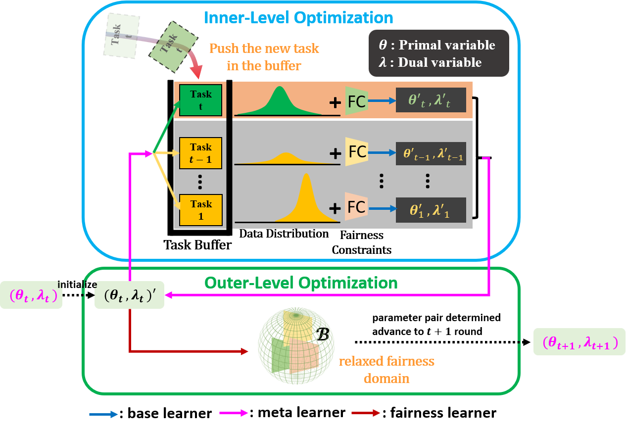
The proposed Algorithm 1 is composed of two levels where each responds for the inner and outer problems stated in Eq.(6) and Eq.(5), respectively. The output of the outer problem are used to define the inner objective function and vice versa. A parameter pair is therefore iteratively updated between the two levels.

To solve the inner level problem stated in Eq.(6), we first consider the following Lagrangian function and omit $\mathcal{D}$ for the sake of brevity:

(7) $$\mathcal{L}_{k}(\boldsymbol{\theta}_{k},\boldsymbol{\lambda}_{k};\boldsymbol{\theta,\lambda})=f_{k}(\boldsymbol{\theta}_{k};\boldsymbol{\theta})+\sum_{i=1}^{m}\lambda_{k,i}g_{i}(\boldsymbol{\theta}_{k};\boldsymbol{\theta})$$

Algorithm 1 The FFML Algorithm

Require: Learning rates $\eta_{1},\eta_{2}$, some constant $\delta$.

1:Randomly initialize primal and dual meta-parameters, $(\boldsymbol{\theta}_{1},\boldsymbol{\lambda}_{1})\in(\Theta\times\mathbb{R}_{+}^{m})$

2:Initialize the task buffer $\mathcal{U}\leftarrow[]$

3:for $t=1,2,...,T$ do

4:     Sample $\mathcal{D}_{t}^{V}\subseteq\mathcal{D}_{t}$ from task $t$

5:     

Evaluate performance of task $t$ using $\mathcal{D}_{t}^{V}$ and $\boldsymbol{\theta}_{t}$

6:     Append $\mathcal{D}_{t}$ to task buffer $\mathcal{U}\leftarrow\mathcal{U}+[\mathcal{D}_{t}]$

7:     if $t\neq 1$ then

8:         Initialize $\boldsymbol{\theta}^{N_{iter}=0}\leftarrow\boldsymbol{\theta}_{t}$ and $\boldsymbol{\lambda}^{N_{iter}=0}\leftarrow\boldsymbol{\lambda}_{t}$

9:         while $N_{iter}=1,2,...$ do

10:              for each task $\mathcal{D}_{k}$ in $\mathcal{U}$ where $k\in[t]$ do

11:                  $\boldsymbol{\theta}_{k}\leftarrow\boldsymbol{\theta}^{N_{iter}-1}$; $\boldsymbol{\lambda}_{k}\leftarrow\boldsymbol{\lambda}^{N_{iter}-1}$

12:                  Sample datapoints $\mathcal{D}_{k}^{S}\subset\mathcal{D}_{k}$

13:                  

Compute adapted task-level primal and dual pair $(\boldsymbol{\theta}^{\prime}_{k},\boldsymbol{\lambda}^{\prime}_{k})$ using Eq.(8) and (9).

14:                  Sample datapoints $\mathcal{D}_{k}^{Q}\subset\mathcal{D}_{k}$

15:                  

Compute $f_{k}(\boldsymbol{\theta}^{\prime}_{k},\mathcal{D}_{k}^{Q})$ and $g_{i}(\boldsymbol{\theta}^{\prime}_{k},\mathcal{D}_{k}^{Q}),\forall i\in[m]$ using $\mathcal{D}_{k}^{Q}$.

16:              end for

17:              

Update meta-level primal-dual parameter pair ($\boldsymbol{\theta}^{N_{iter}},\boldsymbol{\lambda}^{N_{iter}}$) using Eq.(4.2) and (12).

18:         end while

19:         

Set meta-parameters $(\boldsymbol{\theta}_{t},\boldsymbol{\lambda}_{t})\leftarrow(\boldsymbol{\theta}^{N_{iter}},\boldsymbol{\lambda}^{N_{iter}})$

20:     end if

21:     $(\boldsymbol{\theta}_{t+1},\boldsymbol{\lambda}_{t+1})\leftarrow(\boldsymbol{\theta}_{t},\boldsymbol{\lambda}_{t})$

22:end for

where $\boldsymbol{\theta}_{k}\in\mathcal{B}$ is the task-level primal variable initialized with the meta-level primal variable $\boldsymbol{\theta}$, and $\boldsymbol{\lambda}_{k}\in\mathbb{R}^{m}_{+}$ is the corresponding dual variable initialized with $\boldsymbol{\lambda}$, which is used to penalize the violation of constraints. Here, for the purpose of optimization with simplicity, constraints of Eq.(6) are approximated with the cumulative one shown in Eq.(7). To optimize, we update the task-level variables through a base learner $\mathcal{A}lg_{k}(\cdot):\boldsymbol{\theta}_{k}\in\mathcal{B}\rightarrow\boldsymbol{\theta}^{\prime}_{k}\in\mathbb{R}^{d}$. One example for the learner is updating with one gradient step using the pre-determined stepsize $\eta_{1}>0$ (Finn et al., 2019). Notice that for multiple gradient steps, $\boldsymbol{\theta}^{\prime}_{k}$ and $\boldsymbol{\lambda}^{\prime}_{k}$ interplay each other for updating.

(8) $$\boldsymbol{\theta}^{\prime}_{k}=\mathcal{A}lg_{k}(\boldsymbol{\theta}_{k};\boldsymbol{\theta})\triangleq\boldsymbol{\theta}_{k}-\eta_{1}\nabla_{\boldsymbol{\theta}}\mathcal{L}_{k}(\boldsymbol{\theta}_{k},\boldsymbol{\lambda}_{k};\boldsymbol{\theta,\lambda})$$

(9) $$\boldsymbol{\lambda}^{\prime}_{k}=\Big{[}\boldsymbol{\lambda}_{k}+\eta_{1}\nabla_{\boldsymbol{\lambda}}\mathcal{L}_{k}(\boldsymbol{\theta}^{\prime}_{k},\boldsymbol{\lambda}_{k};\boldsymbol{\theta,\lambda})\Big{]}_{+}$$

Next, to solve the outer level problem, the intuition behind our approach stems from the observation that the constrained optimization problem is equivalent to a convex-concave optimization problem with respect to the outer-level primal variable $\boldsymbol{\theta}$ and dual variable $\boldsymbol{\lambda}$. We hence consider the following augmented Lagrangian function:

(10) $$\mathcal{L}_{t}(\boldsymbol{\theta,\lambda})=\frac{1}{t}\sum_{k=1}^{t}\Bigg{\{}f_{k}(\boldsymbol{\theta};\boldsymbol{\theta}^{\prime}_{k})+\sum_{i=1}^{m}\Big{(}\lambda_{i}g_{i}(\boldsymbol{\theta};\boldsymbol{\theta}^{\prime}_{k})-\frac{\delta\eta_{2}}{2}\lambda_{i}^{2}\Big{)}\Bigg{\}}$$

where $\delta>0$ and $\eta_{2}>0$ are some constant and stepsize whose values will be decided by the analysis. Besides, the augmented term on the dual variable is devised to prevent $\boldsymbol{\lambda}$ from being too large (Mahdavi et al., 2012). To optimize the meta-parameter pair in the outer problem, the update rule follows

$$\boldsymbol{\theta}_{t+1} =\prod_{\mathcal{B}}(\boldsymbol{\theta}_{t}-\eta_{2}\nabla_{\boldsymbol{\theta}}\mathcal{L}_{t}(\boldsymbol{\theta}_{t},\boldsymbol{\lambda}_{t}))$$

(11) $$=\arg\min_{\boldsymbol{y}\in\mathcal{B}}||\boldsymbol{y}-(\boldsymbol{\theta}_{t}-\eta_{2}\nabla_{\boldsymbol{\theta}}\mathcal{L}_{t}(\boldsymbol{\theta}_{t},\boldsymbol{\lambda}_{t}))||^{2}$$

(12) $$\boldsymbol{\lambda}_{t+1} =\Big{[}\boldsymbol{\lambda}_{t}+\eta_{2}\nabla_{\boldsymbol{\lambda}}\mathcal{L}_{t}(\boldsymbol{\theta}_{t},\boldsymbol{\lambda}_{t})\Big{]}_{+}$$

where $\prod_{\mathcal{B}}$ is the projection operation to the relaxed domain $\mathcal{B}$ that is introduced in Sec.3.3. This approximates the true desired projection with a simpler closed-form.

We detail the iterative update procedure in Algorithm 1. At round $t\in[T]$, we first evaluate the performance on the new arrived task $\mathcal{D}_{t}$ using $\boldsymbol{\theta}_{t}$ (line 5) and $\mathcal{D}_{t}$ is added to the task buffer $\mathcal{U}$ (line 6). As for the bi-level update, each task-level parameters $\boldsymbol{\theta}_{k},\boldsymbol{\lambda}_{k}$ from the buffer are initialized with the meta-level ones (line 8). In line 13, task-level parameters are updated using support data. Query loss and fairness for each task are further computed in line 15 and they are used to optimize meta parameters in line 17. An overview of the update procedure is described in Figure 1.

Different from techniques devised to solve online learning problems with long-term constraints, at each round FFML finds a good primal-dual parameter pair by learning from prior experience through dealing with a bi-level optimization problem. In order to ensure bias-free predictions, objective functions in both inner and outer levels subject to fairness constraints. Besides, since we generalize the traditional primal-dual update scheme onto a bi-level optimization problem, conventional theoretic guarantees cannot be applied. We hence demonstrate analysis of FFML in the following section.

5. Analysis

To analysis, in this paper, we first make following assumptions as in (Finn et al., 2019) and (Mahdavi et al., 2012). These assumptions are commonly used in meta learning and online learning settings. Examples where these assumptions hold include logistic regression and $L2$ regression over a bounded domain. As for constraints, a family of fairness notions, such as linear relaxation based DDP (Difference of Demographic Parity) including Eq.(2), are applicable as discussed in (Lohaus et al., 2020).

Assumption 1 (Convex domain).

The convex set $\Theta$ is non-empty, closed, bounded, and can be described by $m$ convex functions as $\Theta=\{\boldsymbol{\theta}:g_{i}(\boldsymbol{\theta})\leq 0,\forall i\in[m]\}$

Assumption 2.

Both the loss functions $f_{t}(\cdot),\forall t$ and constraint functions $g_{i}(\cdot),\forall i\in[m]$ satisfy the following assumptions

1. (Lipschitz continuous) $f_{t}(\boldsymbol{\theta}),\forall t$ and $g_{i}(\boldsymbol{\theta}),\forall i$ are Lipschitz continuous in $\mathcal{B}$, that is, $\forall\boldsymbol{\theta,\phi}\in\mathcal{B}$, $||f_{t}(\boldsymbol{\theta})-f_{t}(\boldsymbol{\phi})||\leq L_{f}||\boldsymbol{\theta-\phi}||,||g_{i}(\boldsymbol{\theta})-g_{i}(\boldsymbol{\phi})||\leq L_{g}||\boldsymbol{\theta-\phi}||$, and $G=\max\{L_{f},L_{g}\}$, and

   $$F=\max_{t\in[T]}\max_{\boldsymbol{\theta,\phi}\in\mathcal{B}}f_{t}(\boldsymbol{\theta})-f_{t}(\boldsymbol{\phi})\leq 2L_{f}R$$

   $$D=\max_{i\in[m]}\max_{\boldsymbol{\theta}\in\mathcal{B}}g_{i}(\boldsymbol{\theta})\leq L_{g}R$$

2. (Lipschitz gradient) $f_{t}(\boldsymbol{\theta}),\forall t$ are $\beta_{f}$-smooth and $g_{i}(\boldsymbol{\theta}),\forall i$ are $\beta_{g}$-smooth, that is, $\forall\boldsymbol{\theta,\phi}\in\mathcal{B}$, $||\nabla f_{t}(\boldsymbol{\theta})-\nabla f_{t}(\boldsymbol{\phi})||\leq\beta_{f}||\boldsymbol{\theta-\phi}||,\\ ||\nabla g_{i}(\boldsymbol{\theta})-\nabla g_{i}(\boldsymbol{\phi})||\leq\beta_{g}||\boldsymbol{\theta-\phi}||$, and $H=\max\{\beta_{f},\beta_{g}\}$.

3. (Lipschitz Hessian) Twice-differentiable functions $f_{t}(\boldsymbol{\theta}),\forall t$ and $g_{i}(\boldsymbol{\theta}),\forall i$ have $\rho_{f}$ and $\rho_{g}$- Lipschitz Hessian, respectively. That is, $\forall\boldsymbol{\theta,\phi}\in\mathcal{B}$, $||\nabla^{2}f_{t}(\boldsymbol{\theta})-\nabla^{2}f_{t}(\boldsymbol{\phi})||\leq\rho_{f}||\boldsymbol{\theta-\phi}||,\\ ||\nabla^{2}g_{i}(\boldsymbol{\theta})-\nabla^{2}g_{i}(\boldsymbol{\phi})||\leq\rho_{g}||\boldsymbol{\theta-\phi}||$.

Assumption 3 (Strongly convexity).

Suppose $f_{t}(\boldsymbol{\theta}),\forall t$ and $g_{i}(\boldsymbol{\theta}),\forall i$ have strong convexity, that is, $\forall\boldsymbol{\theta,\phi}\in\mathcal{B}$, $||\nabla f_{t}(\boldsymbol{\theta})-\nabla f_{t}(\boldsymbol{\phi})||\geq\mu_{f}||\boldsymbol{\theta-\phi}||,||\nabla g_{i}(\boldsymbol{\theta})-\nabla g_{i}(\boldsymbol{\phi})||\geq\mu_{g}||\boldsymbol{\theta-\phi}||$.

We then analyze the proposed FFML algorithm and use one-step gradient update as an example. Under above assumptions, we first target Eq.(10) and state:

Theorem 1.

Suppose $f$ and $g:\Theta\times\mathbb{R}_{+}^{m}\rightarrow\mathbb{R}$ satisfy Assumptions 1, 2 and 3. The inner level update and the augmented Lagrangian function $\mathcal{L}_{t}(\boldsymbol{\theta,\lambda})$ are defined in Eq.(8)(7) and Eq.(10). Then, the function $\mathcal{L}_{t}(\boldsymbol{\theta,\lambda})$ is convex-concave with respect to the arguments $\boldsymbol{\theta}$ and $\boldsymbol{\lambda}$, respectively. Furthermore, as for $\mathcal{L}_{t}(\boldsymbol{\cdot,\lambda})$, if stepsize $\eta_{1}$ is selected as $\eta_{1}\leq\min\{\frac{\mu_{f}+\bar{\lambda}m\mu_{g}}{8(L_{f}+\bar{\lambda}mL_{g})(\rho_{f}+\bar{\lambda}m\rho_{g})},\frac{1}{2(\beta_{f}+\bar{\lambda}m\beta_{g})}\}$, then $\mathcal{L}_{t}(\boldsymbol{\cdot,\lambda})$ enjoys $\frac{9}{8}(\beta_{f}+\bar{\lambda}m\beta_{g})$-smooth and $\frac{1}{8}(\mu_{f}+\bar{\lambda}m\mu_{g})$-strongly convex, where $\bar{\lambda}\geq 0$ is the mean value of $\boldsymbol{\lambda}$.

We next present the key Theorem 2. We state that FFML enjoys sub-linear guarantee for both regret and long-term fairness constraints in the long run for Algorithm 1.

Theorem 2.

Set $\eta_{2}=\mu_{f}/(t+1)$ and choose $\delta$ such that $\delta\geq\max\{4m(G^{4}\eta_{1}^{2}m^{2}+\delta^{2}\eta_{2}^{2}),4G^{2}\eta_{1}^{2}H^{2}(m+1)^{2}\}$. If we follow the update rule in Eq.(4.2)(10) and $\boldsymbol{\theta}^{*}$ being the optimal solution for $\min_{\boldsymbol{\theta}\in\Theta}\sum_{t=1}^{T}\\ f_{t}(\mathcal{A}lg_{t}(\boldsymbol{\theta}))$, we have upper bounds for both the regret on the loss and the cumulative constraint violation

$$\sum_{t=1}^{T}\Big{\{}f_{t}(\mathcal{A}lg_{t}(\boldsymbol{\theta}_{t}))-f_{t}(\mathcal{A}lg_{t}(\boldsymbol{\theta}^{*}))\Big{\}}\leq O(\log T)$$

$$\sum_{t=1}^{T}g_{i}(\mathcal{A}lg_{t}(\boldsymbol{\theta}_{t}))\leq O(\sqrt{T\log T}),\forall i\in[m]$$

Regret Discussion: Under aforementioned assumptions and provable convexity of Eq.(10) in $\boldsymbol{\theta}$ (see Theorem 1), Algorithm 1 achieves sublinear bounds for both loss regret and violation of fairness constraints (see Theorem 2) where $\lim_{T\rightarrow\infty}O(\cdot)/T=0$. Although such bounds are comparable with cutting-edge techniques of online learning with long-term constraints (Yuan and Lamperski, 2018; Jenatton et al., 2016) in the case of strongly convexity, in terms of online meta-learning paradigms, for the first time we bound loss regret and cumulative fairness constraints simultaneously. For space purposes, proofs for all theorems are contained in the Appendix A and B.

6. Experiments

To corroborate our algorithm, we conduct extensive experiments comparing FFML with some popular baseline methods. We aim to answer the following questions:

1. Question 1: Can FFML achieve better performance on both fairness and classification accuracy compared with baseline methods?

2. Question 2: Can FFML be successfully applied to non-stationary learning problems and achieve a bounded fairness as $t$ increases?

3. Question 3: How efficient is FFML in task evaluation over time and how is the contribution for each component?

6.1. Datasets

We use the following three publicly available datasets. Each dataset contains a sequence of tasks where the ordering of tasks is selected at random. (1) Bank Marketing (Moro et al., 2014) contains a total 41,188 subjects, each with 16 attributes and a binary label, which indicates whether the client has subscribed or not to a term deposit. We consider the marital status as the binary protected attribute. The dataset contains 50 tasks and each corresponds to a date when the data are collected from April to December in 2013. (2) Adult (Kohavi and Becker, 1994) is broken down into a sequence of 41 income classification tasks, each of which relates to a specific native country. The dataset totally 48,842 instances with 14 features and a binary label, which indicates whether a subject’s incomes is above or below 50K dollars. We consider gender, i.e. male and female, as the protected attribute. (3) Communities and Crime (Lichman, 2013) is split into 43 crime classification tasks where each corresponds to a state in the U.S. Following the same setting in (Slack et al., 2020), we convert the violent crime rate into binary labels based on whether the community is in the top $50\%$ crime rate within a state. Additionally, we add a binary protected attribute that receives a protected label if African-Americans are the highest or second highest population in a community in terms of percentage racial makeup.

6.2. Evaluation Metrics

Three popular evaluation metrics are introduced that each allows quantifying the extent of bias taking into account the protected attribute.

Demographic Parity (DP) (Dwork et al., 2011) and Equalized Odds (EO) (Hardt et al., 2016) can be formalized as

$$\text{DP}=\frac{P(\hat{Y}=1|S=0)}{P(\hat{Y}=1|S=1)};\quad\text{EO}=\frac{P(\hat{Y}=1|S=0,Y=y)}{P(\hat{Y}=1|S=1,Y=y)}$$

where $y\in\{0,1\}$. Equalized odds requires that $\hat{Y}$ have equal true positive rates and false positive rates between sub-groups. For both metrics, a value closer to 1 indicate fairness.

Discrimination (Zemel et al., 2013) measures the bias with respect to the protected attribute $S$ in the classification:

$$\text{Disc}=\Bigg{|}{\frac{\sum_{i:s_{i}=1}\hat{y}_{i}}{\sum_{i:s_{i}=1}1}-\frac{\sum_{i:s_{i}=0}\hat{y}_{i}}{\sum_{i:s_{i}=0}1}}\Bigg{|}$$

This is a form of statistical parity that is applied to the binary classification decisions. We re-scale values across all baseline methods into a range of $[0,1]$ and $Disc=0$ indicates there is no discrimination.

Table 2. End task performance on real datasets over all baseline methods. Evaluation metrics with ”$\uparrow$” indicates the bigger the better and ”$\downarrow$” indicates the smaller the better. Best performance are labeled in bold.

Dataset	DP $\uparrow$	EO $\uparrow$	Disc $\downarrow$	Acc($\%$) $\uparrow$
	TWP / m-FTML(Finn et al., 2019) / OGDLC(Mahdavi et al., 2012) / AdpOLC(Jenatton et al., 2016) / GenOLC(Yuan and Lamperski, 2018) / FFML(Ours)
Bank	0.09/0.68/0.36/0.76/0.81/0.97	0.11/0.65/0.35/0.72/0.78/0.96	0.19/0.72/0.23/0.22/0.11/0.07	52.14/53.69/52.36/54.89/56.78/52.55
Adult	0.05/0.54/0.41/0.60/0.78/0.91	0.04/0.43/0.30/0.62/0.69/0.87	0.32/0.69/0.21/0.19/0.12/0.10	51.21/67.91/52.31/48.36/47.87/61.35
Crime	0.40/0.38/0.48/0.68/0.70/0.74	0.38/0.29/0.39/0.43/0.64/0.69	0.23/0.78/0.25/0.31/0.15/0.17	51.23/48.69/49.10/58.89/49.43/59.57

6.3. Competing Methods

(1) Train with penalty (TWP): is an intuitive approach for online fair learning where loss functions at each round is penalized by the violation of fairness constraints. We then run the standard online gradient descent (OGD) algorithm to minimize the modified loss function. (2) m-FTML (Finn et al., 2019): the original FTML finds a sequence of meta parameters by simply applying MAML (Finn et al., 2017) at each round. To focus on fairness learning, this approach is applied to modified datasets by removing protected attributes. Notice that techniques (3)-(5) are proposed for online learning with long-term constraints and achieve state-of-the-art performance in theoretic guarantees. In order to fit bias-prevention and compare them to FFML, we specify such constraints as DBC stated in Eq.(2). (3) OGDLC (Mahdavi et al., 2012): updates parameters solely based on the on-going task. (4) AdpOLC (Jenatton et al., 2016): improves OGDLC by modifying stepsizes to an adapted version. (5) GenOLC (Yuan and Lamperski, 2018): rectifies AdpOLC by square-clipping the constraints in place of $g_{i}(\cdot),\forall i$. Although OGDLC, AdpOLC and GenOLC are devised for online learning with long-term constraints, none of these state-of-the-arts considers inner-level adaptation. We note that, among the above baseline methods, m-FTML is a state-of-the-art one in the the area of online meta learning. The last three baselines, including OGDLC, AdpOLC, GenOLC are representative ones in the area of online optimization with long term constraints.

Figure 2. Evaluation using fair metric DP at each round.

Figure 3. Evaluation using fair metric EO at each round.

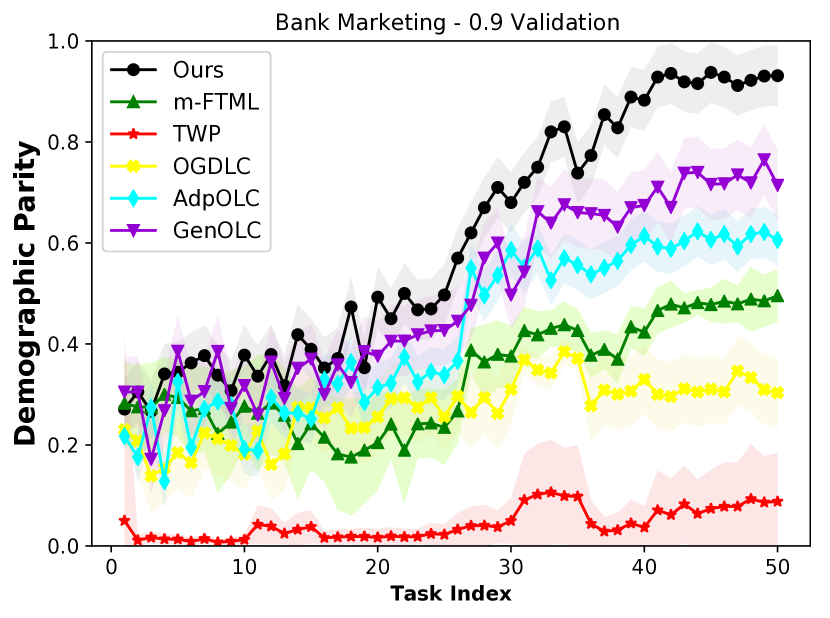
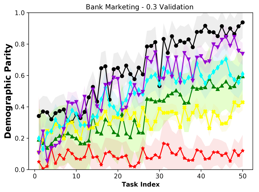
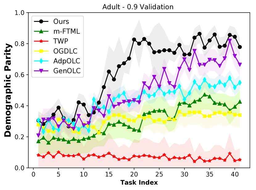
6.4. Settings

As discussed in Sec.5, the performance of our proposed method has been well justified theoretically for machine learning models, such as logistic regression and L2 regression, whose objectives that are strongly convex and smooth. However, in machine learning and fairness studies, due to the non-linearity of neural networks, many problems have a non-convex landscape where theoretical analysis is challenging. Nevertheless, algorithms originally developed for convex optimization problems like gradient descent have shown promising results in practical non-convex settings (Finn et al., 2019). Taking inspiration from these successes, we describe practical instantiations for the proposed online algorithm, and empirically evaluate the performance in Sec.7.

Figure 4. Amount of data needed to learn each new task.

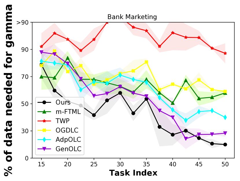
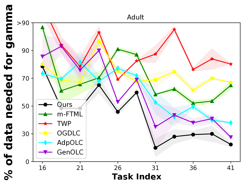
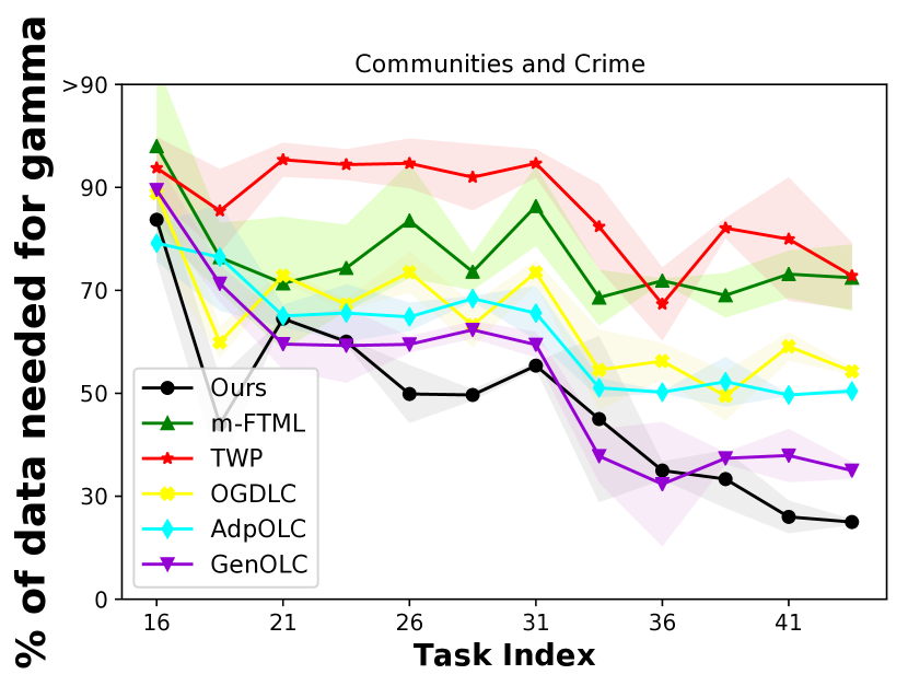
For each task we set the number of fairness constraints to one, i.e. $m=1$. For the rest, we following the same settings as used in online meta learning (Finn et al., 2019). In particular, we meta-train with support size of 100 for each class, whereas $30\%$ or $90\%$ (hundreds of datapoints) of task samples for evaluation. All methods are completely online, i.e., all learning algorithms receive one task per-iteration. All the baseline models that are used to compare with our proposed approach share the same neural network architecture and parameter settings. All the experiments are repeated 10 times with the same settings and the mean and standard deviation results are reported. Details on the settings are given in Appendix C.

7. Results

The following experimental results on each dataset are to answer all Questions given in Sec.6.

7.1. End Task Performance

In contrast to traditional machine learning paradigms where they often run a batch learning fashion, online learning aims to learn and update the best predictor for future data at each round. In our experiments, we consider a sequential setting where a task comes one after another. To validate the effectiveness of the proposed algorithm, we first compare the end task performance. All methods stop at $t=T$ after seeing all tasks. The learned parameter pair $(\boldsymbol{\theta}_{T},\boldsymbol{\lambda}_{T})$ is further fine-tuned using the support set $\mathcal{D}_{T}^{S}$ which is sampled from the task $T$. The end task performance is hence evaluated on the validation set $\mathcal{D}_{T}^{V}$ using the adapted parameter $\boldsymbol{\theta}^{\prime}_{T}$.

Consolidated and detailed performance of the different techniques over real-world data are listed in Table 2. We evaluate performance across all competing methods on a scale of $90\%$ datapoints of the end task $T$ for each dataset. Best performance in each experimental unit are labeled in bold. We observe that as for bias-controlling, FFML out-performs than other baseline methods. Specifically, FFML has the highest scores in terms of the fairness metrics DP and EO, and the smallest value of Disc close to zero signifies a fair prediction. Note that although FFML returns a bit smaller predictive accuracy, this is due to the trade-off between losses and fairness.

7.2. Performance Through Each Round

In order to take a closer look at the performance regarding bias-control in a non-stationary environment, at round $t\in[T]$, the parameter pair $(\boldsymbol{\theta}_{t},\boldsymbol{\lambda}_{t})$ inherited from the previous task $t-1$ are employed to evaluate the new task $t$. Inspired by (Finn et al., 2019), we separately record the performance based on different amount (i.e. $90\%$ and $30\%$) of validation samples.

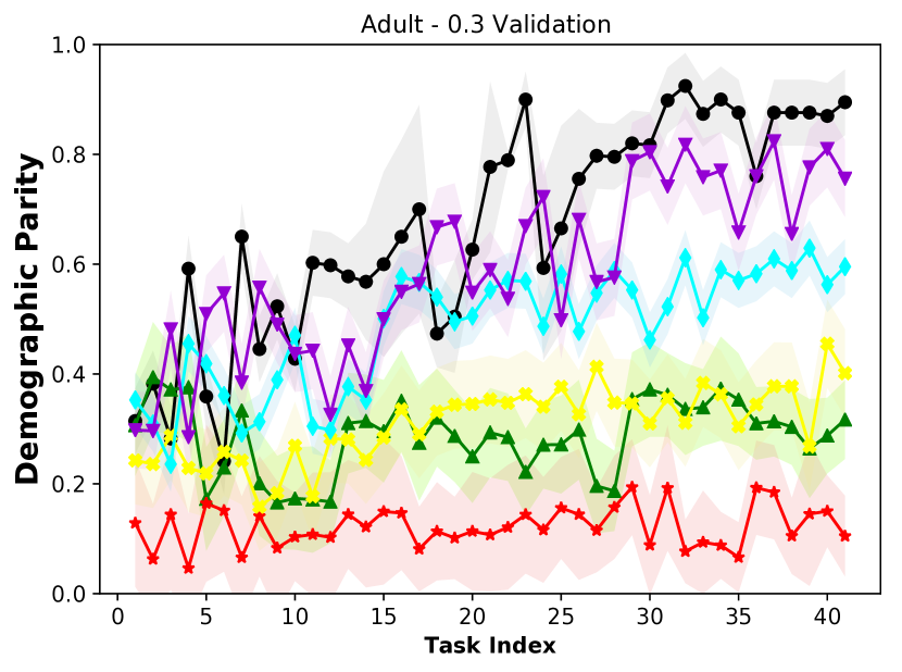
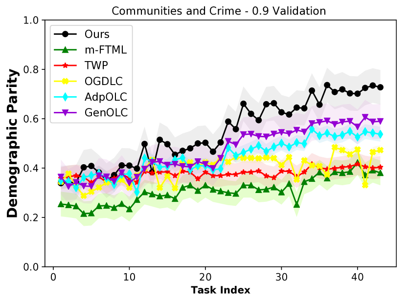
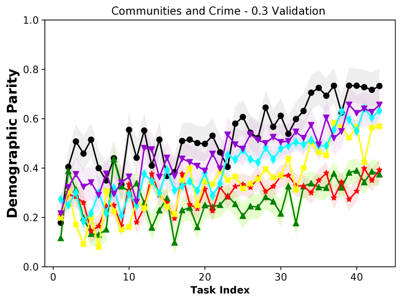
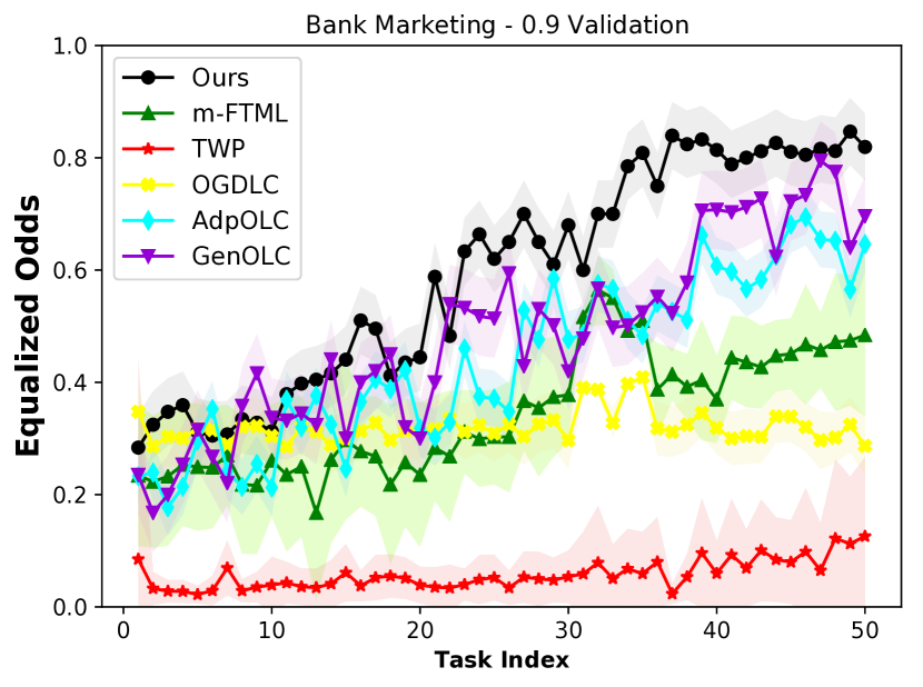
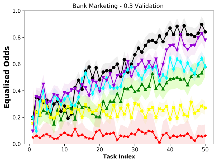
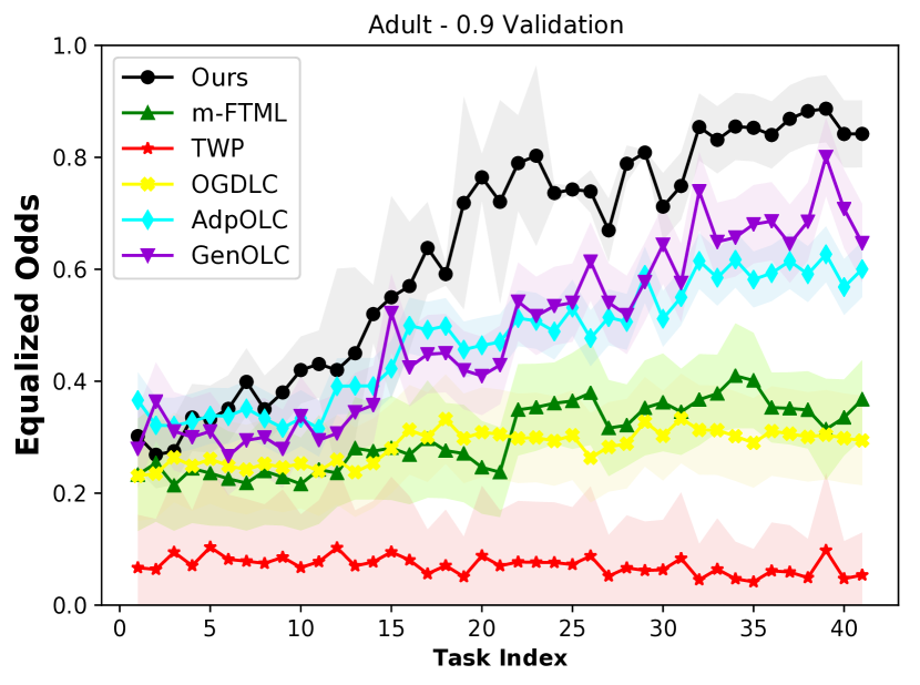
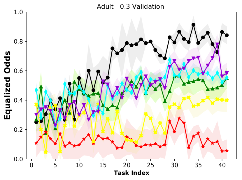
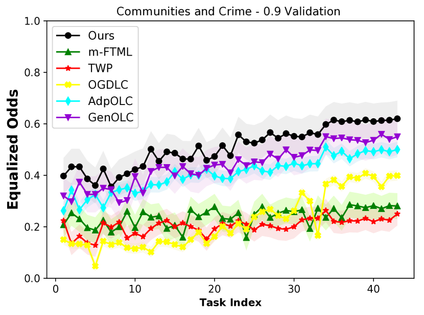
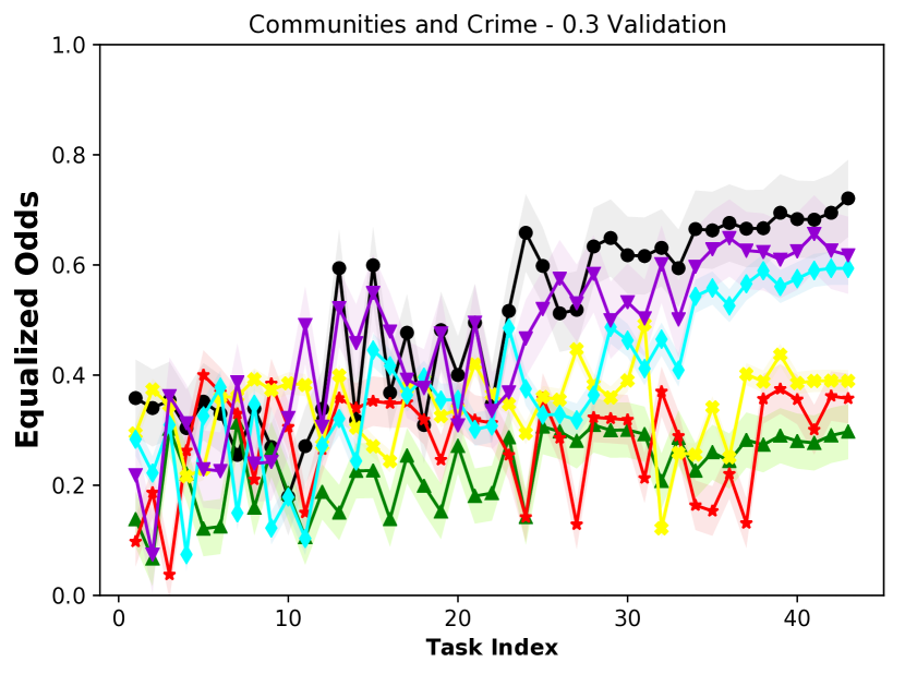
Figure 2 and 3 detail evaluation results across three real-world datasets at each round with respect to two wildly used fairness metrics DP and EO, respectively. Specifically, higher is better for all plots, while shaded regions show standard error computed using various random seeds. The learning curves show that with each new task added FFML efficiently controls bias and substantially outperforms the alternative approaches in achieving the best fairness aware results represented by the highest $DP$ and $EO$ in final performance. GenOLC returns better results than AdpOLC and OGDLC since it applies both adaptive learning rates and squared clipped constraint term. However, two of the reasons giving rise to the performance of GenOLC inferior to FFML is that our method (1) takes task-specific adaptation with respect to primal-dual parameter pair at inner loops, which further helps the task progress better as for fairness learning, (2) FFML explicitly meta-trains and hence fully learns the structure across previous seen tasks. Although m-FTML shows an improvement in fairness, there is still substantial unfairness hidden in the data in the form of correlated attributes, which is consistent with (Zemel et al., 2013) and (Lahoti et al., 2019). As the most intuitive approach, theoretic analysis in (Mahdavi et al., 2012) shown the failure of using TWP is that the weight constant is fixed and independent from the sequences of solutions obtained so far.

Another observation is when evaluation data are reduced to $30\%$. Although the fairness performance becomes more fluctuant, FFML remains the out-performance than other baseline methods through each round. This results from that in a limited amount of evaluated data our method stabilizes the results by learning parameters from all prior tasks so far at each round, and suggests that even better transfer can be accomplished through meta-learning.

7.3. Task Learning Efficiency

To validate the learning efficiency of the proposed FFML, we set a proficiency threshold $\boldsymbol{\gamma}$ for all methods at each round, where $\boldsymbol{\gamma}=(\gamma_{1},\gamma_{2})$ corresponds to the amount of data needed in $\mathcal{D}_{t}$ to achieve both a loss value $f_{t}(\boldsymbol{\theta}_{t},\mathcal{D}_{t}^{V})\leq\gamma_{1}$ and a DBC value $g_{t}(\boldsymbol{\theta}_{t},\mathcal{D}_{t}^{V})\leq\gamma_{2}$ at the same time. We set $\gamma_{1}=0.0005$ and $\gamma_{2}=0.0001$ for all datasets. If less data is sufficient to reach the threshold, then priors learned from previous tasks are being useful and we have achieved positive transfer (Finn et al., 2019). Through the results demonstrated in Figure 4, we observe while the baseline methods improve in efficiency over the course of learning as they see more tasks, they struggle to prevent negative transfer on each new task.

7.4. Ablation Studies

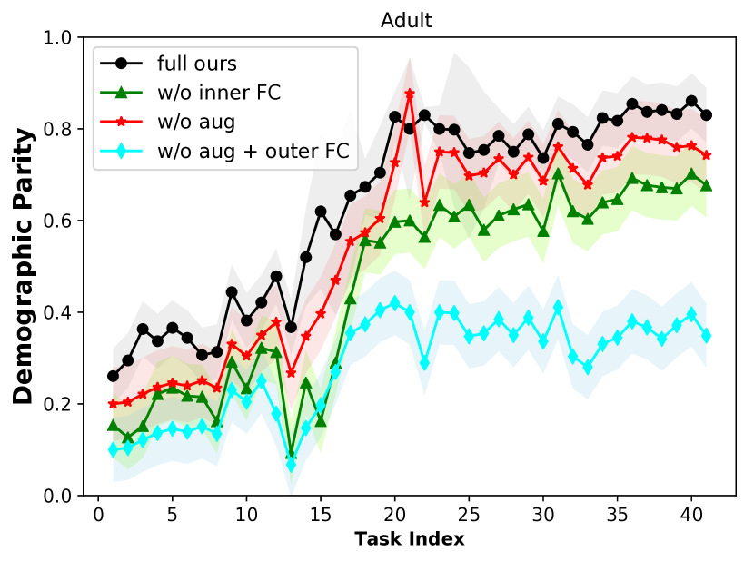
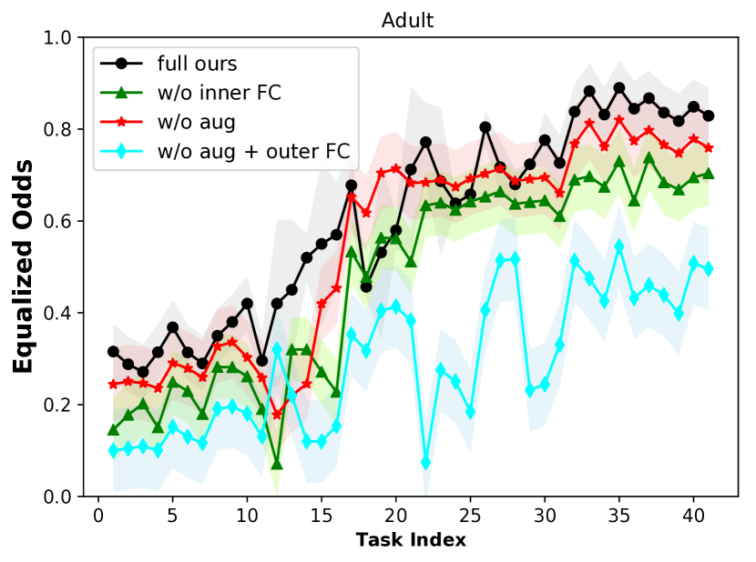
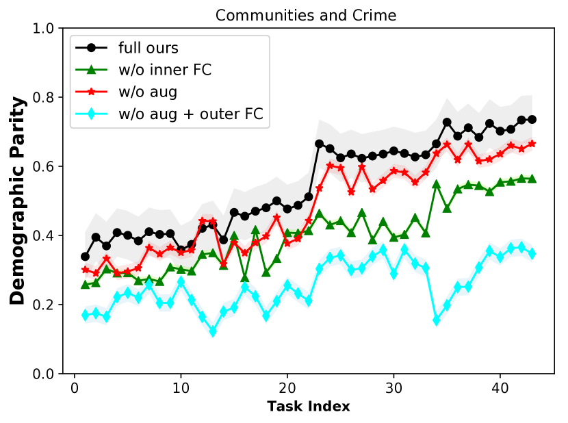
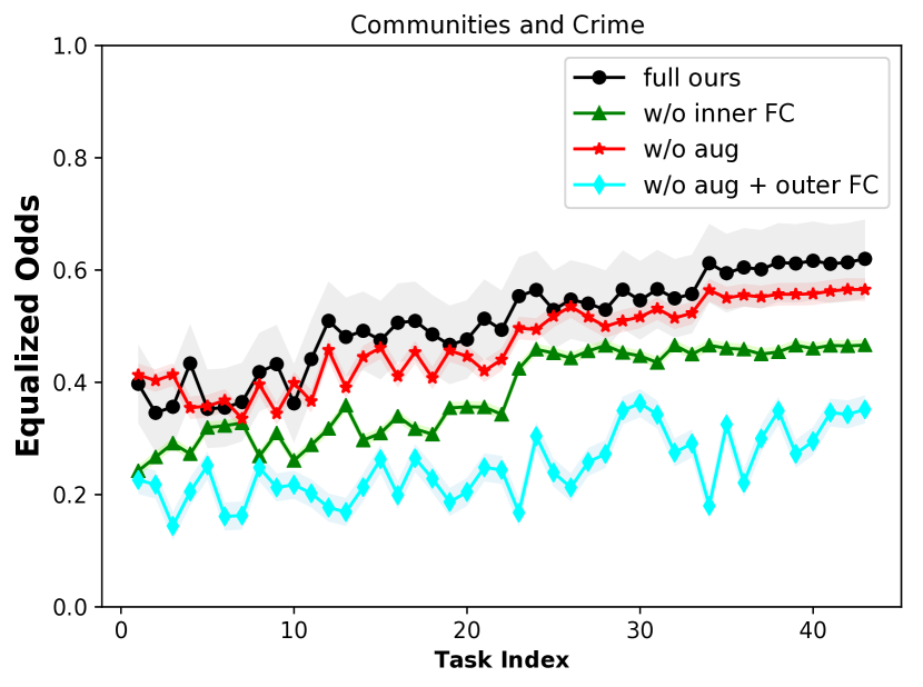
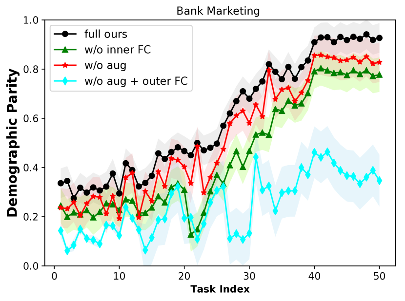
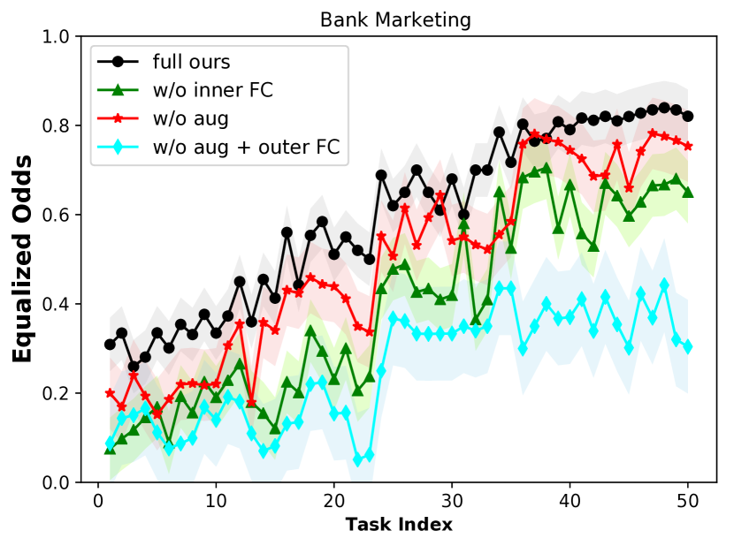
We conducted additional experiments to demonstrate the contributions of the three key technical components in FFML: the inner(task)-level fairness constraints (inner FC) in Eq.(6), the outer (meta)-level fairness constraints (outer FC) in Eq.(7), and the augmented term (aug) in Eq.(10). Particularly, Inner FC and outer FC are used to regularize the task-level and metal-level loss functions, respectively, and aug is used to prevent the dual parameters being to large and hence stabilizes the learning with fairness in the outer problem. The key findings in Figure 5 are (1) inner fairness constraints and the augmented term can enhance bias control, and (2) outer update procedure plays more important role in FFML. This is due to the close-form projection onto the relaxed domain $\mathcal{B}$ with respect to primal variable and clipped non-negative dual variable.

Figure 5. Ablation study of our proposed models. (1) w/o inner FC: FFML without inner fairness constraints; (2) w/o aug: FFML without the augmented term in Eq.(10); (3) w/o aug + outer FC: FFML without the augmented term and outer fairness constraints.

8. Conclusion and Future Work

In this paper, we formulate the problem of online fairness-aware meta learning and present a novel algorithm, namely FFML. We claim that for the first time a fairness-aware online meta-learning framework is proposed. The goal of this model is to minimize both the loss regret and violation of long-term fairness constraints as $t$ increases, and to achieve sub-linear bound for them. Specifically, in stead of learning primal parameters only at each round, FFML trains a meta-parameter pair including primal and dual variables, where the primal variable determines the predictive accuracy and the dual variable controls the level of satisfaction of model fairness. To determine the parameter pair at each round, we formulate the problem to a bi-level convex-concave optimization problem. Detailed theoretic analysis and corresponding proofs justify the efficiency and effectiveness of the proposed algorithm by demonstrating upper bounds for regret and violation of fairness constraints. Experimental evaluation based on three real-world datasets shows that our method out-performs than state-of-the-art online learning techniques with long-term fairness constraints in bias-controlling. It remains interesting if one can prove that fairness constraints are satisfied at each round without approximated projections onto the relaxed domain, and if one can explore learning when environment is changing over time.

Appendix A Sketch of Proof of Theorem 1

Proof.

Before giving the proof of Theorem 1, let us define a function $\tilde{\mathcal{L}}(\boldsymbol{\theta,\lambda}):(\mathcal{B}\times\mathbb{R}^{m}_{+})\rightarrow\mathbb{R}$ with respect to the primal and dual variable $\boldsymbol{\theta}$ and $\boldsymbol{\lambda}$. Therefore, $\tilde{\mathcal{L}}(\boldsymbol{\theta,\lambda})$ is considered as a single task function $k\in[t]$ from prior experience and it is stripped from Eq.(10).

$$\tilde{\mathcal{L}}(\boldsymbol{\theta,\lambda}) :=\mathcal{L}^{\prime}\Big{(}\mathcal{A}lg(\boldsymbol{\theta}),\boldsymbol{\lambda}\Big{)}$$

$$=f(\mathcal{A}lg(\boldsymbol{\theta}))+\sum\nolimits_{i=1}^{m}\Big{(}\lambda_{i}g_{i}(\mathcal{A}lg(\boldsymbol{\theta}))-\frac{\delta\eta_{2}}{2}\lambda)_{i}^{2}\Big{)}$$

where $\mathcal{A}lg(\boldsymbol{\theta})$ is defined in Eq.(8). We hence first prove $\tilde{\mathcal{L}}(\boldsymbol{\cdot,\lambda})$ is convex with respect to $\boldsymbol{\theta}$. Similar results can be easily achieved with respect to $\boldsymbol{\lambda}$. We consider two arbitrary point $\boldsymbol{\theta,\phi}\in\mathcal{B}$ with respect to the primal variable:

$$||\nabla_{\boldsymbol{\theta}}\tilde{\mathcal{L}}(\boldsymbol{\theta})-\nabla_{\boldsymbol{\phi}}\tilde{\mathcal{L}}(\boldsymbol{\phi})||$$

$$\leq \underbrace{||\nabla_{\boldsymbol{\theta}^{\prime}}\mathcal{L}^{\prime}(\mathcal{A}lg(\boldsymbol{\theta}))(\nabla_{\boldsymbol{\theta}}\mathcal{A}lg(\boldsymbol{\theta})-\nabla_{\boldsymbol{\phi}}\mathcal{A}lg(\boldsymbol{\phi}))||}_{\textbf{First Term (FT)}}+$$

$$\underbrace{||\nabla_{\boldsymbol{\phi}}\mathcal{A}lg(\boldsymbol{\phi})(\nabla_{\boldsymbol{\theta}^{\prime}}\mathcal{L}^{\prime}(\mathcal{A}lg(\boldsymbol{\theta}))-\nabla_{\boldsymbol{\phi}^{\prime}}\mathcal{L}^{\prime}(\mathcal{A}lg(\boldsymbol{\phi})))||}_{\textbf{Second Term (ST)}}$$

We then bound the first and second terms that:

$$\text{FT}\leq \eta_{1}||\nabla_{\boldsymbol{\theta}^{\prime}}\mathcal{L}^{\prime}(\mathcal{A}lg(\boldsymbol{\theta}))||||(\nabla^{2}_{\boldsymbol{\theta}}f(\boldsymbol{\theta})-\nabla^{2}_{\boldsymbol{\phi}}f(\boldsymbol{\phi}))+$$

$$(\nabla^{2}_{\boldsymbol{\theta}}\sum\nolimits_{i=1}^{m}\lambda_{i}g_{i}(\boldsymbol{\theta})-\nabla^{2}_{\boldsymbol{\phi}}\sum\nolimits_{j=1}^{m}\lambda_{j}g_{j}(\boldsymbol{\phi}))||$$

$$\leq \eta_{1}(L_{f}+\bar{\lambda}mL_{g})(\rho_{f}+\bar{\lambda}m\rho_{g})||\boldsymbol{\theta}-\boldsymbol{\phi}||$$

$$\text{ST}= ||(\boldsymbol{I}-\eta_{1}(\nabla^{2}_{\boldsymbol{\phi}}f(\boldsymbol{\phi})+\nabla^{2}_{\boldsymbol{\phi}}\sum\nolimits_{i=1}^{m}\lambda_{i}g_{i}(\boldsymbol{\phi})))$$

$$(\nabla_{\boldsymbol{\theta}^{\prime}}\mathcal{L}^{\prime}(\mathcal{A}lg(\boldsymbol{\theta}))-\nabla_{\boldsymbol{\phi}^{\prime}}\mathcal{L}^{\prime}(\mathcal{A}lg(\boldsymbol{\phi})))||$$

$$\leq (1-\eta_{1}(\mu_{f}+\bar{\lambda}m\mu_{g}))^{2}(\beta_{f}+\bar{\lambda}m\beta_{g})||\boldsymbol{\theta}-\boldsymbol{\phi}||$$

The inequality to bound ST is due to the Lemma 2 to 4 in (Finn et al., 2019). Together the upper bounds for the first and the second terms and choose step size

$$\eta_{1}\leq\min\Big{\{}\frac{\mu_{f}+\bar{\lambda}m\mu_{g}}{8(L_{f}+\bar{\lambda}mL_{g})(\rho_{f}+\bar{\lambda}m\rho_{g})},\frac{1}{2(\beta_{f}+\bar{\lambda}m\beta_{g})}\Big{\}}$$

Then we have

$$||\nabla_{\boldsymbol{\theta}}\tilde{\mathcal{L}}(\boldsymbol{\theta})-\nabla_{\boldsymbol{\phi}}\tilde{\mathcal{L}}(\boldsymbol{\phi})||\leq\frac{9}{8}(\beta_{f}+\bar{\lambda}m\beta_{g})||\boldsymbol{\theta}-\boldsymbol{\phi}||$$

Therefore $\tilde{\mathcal{L}}(\cdot,\boldsymbol{\lambda})$ is $\frac{9}{8}(\beta_{f}+\bar{\lambda}m\beta_{g})$-smooth. Next to achieve lower bound for $\tilde{\mathcal{L}}(\cdot,\boldsymbol{\lambda})$

$$||\nabla_{\boldsymbol{\theta}}\tilde{\mathcal{L}}(\boldsymbol{\theta})-\nabla_{\boldsymbol{\phi}}\tilde{\mathcal{L}}(\boldsymbol{\phi})||$$

$$\geq \underbrace{||\nabla_{\boldsymbol{\phi}}\mathcal{A}lg(\boldsymbol{\phi})(\nabla_{\boldsymbol{\theta}^{\prime}}\mathcal{L}^{\prime}(\mathcal{A}lg(\boldsymbol{\theta}))-\nabla_{\boldsymbol{\phi}^{\prime}}\mathcal{L}^{\prime}(\mathcal{A}lg(\boldsymbol{\phi})))||}_{\textbf{Third Term (TT)}}-$$

$$||\nabla_{\boldsymbol{\theta}^{\prime}}\mathcal{L}^{\prime}(\mathcal{A}lg(\boldsymbol{\theta}))(\nabla_{\boldsymbol{\theta}}\mathcal{A}lg(\boldsymbol{\theta})-\nabla_{\boldsymbol{\phi}}\mathcal{A}lg(\boldsymbol{\phi}))||$$

The second term in the above inequality is the same as the FT. We hence bound the TT that:

TT $$\geq(1-\eta_{1}(\beta_{f}+\bar{\lambda}m\beta_{g}))^{2}(\mu_{f}+\bar{\lambda}m\mu_{g})||\boldsymbol{\theta}-\boldsymbol{\phi}||$$

$$\geq\frac{\mu_{f}+\bar{\lambda}m\mu_{g}}{4}||\boldsymbol{\theta}-\boldsymbol{\phi}||$$

Together TT and FT, we derive the lower bound

$$||\nabla_{\boldsymbol{\theta}}\tilde{\mathcal{L}}(\boldsymbol{\theta})-\nabla_{\boldsymbol{\phi}}\tilde{\mathcal{L}}(\boldsymbol{\phi})||\geq\frac{\mu_{f}+\bar{\lambda}m\mu_{g}}{8}||\boldsymbol{\theta}-\boldsymbol{\phi}||$$

Thus, $\tilde{\mathcal{L}}(\cdot,\boldsymbol{\lambda})$ is $\frac{1}{8}(\mu_{f}+\bar{\lambda}m\mu_{g})$-strongly convex. Since $\tilde{\mathcal{L}}(\cdot,\boldsymbol{\lambda})$ is convex, summation of convex functions with non-negative weights preserves convexity and summation of strongly convex functions is strongly convex. Therefore, we complete the proof for $\mathcal{L}(\cdot,\boldsymbol{\lambda})$. ∎

Appendix B Sketch of Proof of Theorem 2

In order to better understand Theorem 2, we first introduce Lemma 1 and its analysis is modified and analogous to that developed in (Mahdavi et al., 2012).

Lemma 1.

Let $\mathcal{L}_{t}(\cdot,\cdot)$ be the function defined in Eq.(10), which is convex in its first argument and concave in its second argument. Let $\boldsymbol{\theta}_{t}$ and $\boldsymbol{\lambda}_{t},t\in[T]$ be the sequence of solution obtained by Algorithm 1. Then for any $(\boldsymbol{\theta,\lambda})\in\mathcal{B}\times\mathbb{R}^{m}_{+}$, we have

(13) $$\sum\nolimits_{t=1}^{T}\mathcal{L}_{t}(\boldsymbol{\theta}_{t},\boldsymbol{\lambda})-\mathcal{L}_{t}(\boldsymbol{\theta},\boldsymbol{\lambda}_{t})\leq\frac{R^{2}+||\boldsymbol{\lambda}||^{2}}{2\eta_{2}}-\frac{\mu_{f}}{2}R^{2}$$

$$+\sum\nolimits_{t=1}^{T}\Big{\{}\frac{\eta_{2}}{2}\Big{(}4G^{2}\eta_{1}^{2}H^{2}(m+1)^{2}+4m(D^{2}+\eta_{1}^{2}G^{4})\Big{)}$$

$$+2\eta_{2}m(G^{4}\eta_{1}^{2}m^{2}+\delta^{2}\eta_{2}^{2})||\boldsymbol{\lambda}_{t}||^{2}+2\eta_{2}G^{2}\eta_{1}^{2}H^{2}(m+1)^{2}||\boldsymbol{\lambda}_{t}||^{4}\Big{\}}$$

Proof.

Following the Assumption 3 and analysis of the Lemma 2 in (Mahdavi et al., 2012), we derive

$$\mathcal{L}_{t}(\boldsymbol{\theta}_{t},\boldsymbol{\lambda})-\mathcal{L}_{t}(\boldsymbol{\theta},\boldsymbol{\lambda}_{t})\leq\frac{1}{2\eta_{2}}\Big{(}||\boldsymbol{\theta}-\boldsymbol{\theta}_{t}||^{2}+||\boldsymbol{\lambda}-\boldsymbol{\lambda}_{t}||^{2}$$

$$-||\boldsymbol{\theta}-\boldsymbol{\theta}_{t+1}||^{2}-||\boldsymbol{\lambda}-\boldsymbol{\lambda}_{t+1}||^{2}\Big{)}+\frac{\eta_{2}}{2}\Big{(}||\nabla_{\boldsymbol{\theta}}\mathcal{L}_{t}(\boldsymbol{\theta}_{t},\boldsymbol{\lambda}_{t})||^{2}$$

$$+\nabla_{\boldsymbol{\lambda}}\mathcal{L}_{t}|\boldsymbol{\theta}_{t},\boldsymbol{\lambda}_{t}||^{2}\Big{)}-\frac{\mu_{f}}{2}||\boldsymbol{\theta}-\boldsymbol{\theta}_{t}||^{2}$$

We bound $||\nabla_{\boldsymbol{\theta}}\mathcal{L}_{t}(\boldsymbol{\theta}_{t},\boldsymbol{\lambda}_{t})||^{2}\leq 4G^{2}\eta_{1}^{2}H^{2}(m+1)^{2}(1+||\boldsymbol{\lambda}_{t}||^{4})$ and $\nabla_{\boldsymbol{\lambda}}\mathcal{L}_{t}|\boldsymbol{\theta}_{t},\boldsymbol{\lambda}_{t}||^{2}\leq 4m(D^{2}+G^{4}\eta_{1}^{2}m^{2}||\boldsymbol{\lambda}_{t}||^{2}+\delta^{2}\eta_{2}^{2}||\boldsymbol{\lambda}_{t}||^{2}+\eta_{1}^{2}G^{4})$ using the inequality $(a_{1}+a_{2}+\cdots+a_{n})^{2}\leq n(a_{1}^{2}+a_{2}^{2}+\cdots+a_{n}^{2})$. By adding the inequalities of FT and ST, and using the fact $||\boldsymbol{\theta}||\leq R$ and $t\geq 1$ we complete the proof. ∎

By applying Lemma 1, we now prove Theorem 2.

Proof.

By expanding Eq.(13) using Eq.(10), and in short we use RHS to substitute the right-hand side of the inequality of Eq.(13) and set $\boldsymbol{\theta}=\boldsymbol{\theta}^{*}$. Following the Theorem 3.1 in (Cesa-Bianchi and Lugosi, 2006), we have

$$\sum\nolimits_{t=1}^{T}\Big{\{}f_{t}(\mathcal{A}lg_{t}(\boldsymbol{\theta}_{t}))-f_{t}(\mathcal{A}lg_{t}(\boldsymbol{\theta}^{*}))\Big{\}}$$

$$+\sum\nolimits_{i=1}^{m}\Big{\{}\lambda_{i}\sum\nolimits_{t=1}^{T}g_{i}(\mathcal{A}lg_{t}(\boldsymbol{\theta}_{t}))-\sum\nolimits_{t=1}^{T}\lambda_{t,i}g_{i}(\mathcal{A}lg_{t}(\boldsymbol{\theta}^{*}))\Big{\}}$$

$$-\frac{\delta\eta_{2}T}{2}||\boldsymbol{\lambda}||^{2}+\frac{\delta\eta_{2}}{2}\sum\nolimits_{t=1}^{T}||\boldsymbol{\lambda}||^{2}\leq RHS$$

Since $\delta\geq\max\{4m(G^{4}\eta_{1}^{2}m^{2}+\delta^{2}\eta_{2}^{2}),4G^{2}\eta_{1}^{2}H^{2}(m+1)^{2}\}$, we can drop terms containing $||\boldsymbol{\lambda}_{t}||^{2}$ and $||\boldsymbol{\lambda}_{t}||^{4}$. By taking maximization for $\boldsymbol{\lambda}$ over $(0,+\infty)$, we get

$$\sum\nolimits_{t=1}^{T}\Big{\{}f_{t}(\mathcal{A}lg_{t}(\boldsymbol{\theta}_{t}))-f_{t}(\mathcal{A}lg_{t}(\boldsymbol{\theta}^{*}))\Big{\}}$$

$$+\sum\nolimits_{i=1}^{m}\Big{\{}\frac{\Big{[}\sum\nolimits_{t=1}^{T}g_{i}(\mathcal{A}lg_{t}(\boldsymbol{\theta}_{t}))\Big{]}^{2}_{+}}{2(\delta\eta_{2}T+\frac{m}{\eta_{2}})}-\sum\nolimits_{t=1}^{T}\lambda_{t,i}g_{i}(\mathcal{A}lg_{t}(\boldsymbol{\theta}^{*}))\Big{\}}$$

$$\leq\frac{R^{2}}{2\eta_{2}}-\frac{\mu_{f}}{2}R^{2}$$

$$+\Big{(}4G^{2}\eta_{1}^{2}H^{2}(m+1)^{2}+2\zeta^{2}+4m(D^{2}+\eta_{1}^{2}G^{4})\Big{)}\sum\nolimits_{t=1}^{T}\frac{\eta_{2}}{2}$$

Since $g_{i}(\mathcal{A}lg(\boldsymbol{\theta}^{*}))\leq 0$ and $\lambda_{t,i}\geq 0,\forall i\in[m]$. For $f_{t}(\boldsymbol{\theta})$ to be strongly convex, in order to have lower upper bounds for both objective regret and the long-term constraint, we need to use time-varying stepsize as the one used in (Yuan and Lamperski, 2018), that is $\eta_{2}=\mu_{f}/(t+1)$. Due to non-negative of $\frac{\Big{[}\sum\nolimits_{t=1}^{T}g_{i}(\mathcal{A}lg_{t}(\boldsymbol{\theta}_{t}))\Big{]}^{2}_{+}}{2(\delta\eta_{2}T+\frac{m}{\eta_{2}})}$, we have

$$\sum\nolimits_{t=1}^{T}\Big{\{}f_{t}(\mathcal{A}lg_{t}(\boldsymbol{\theta}_{t}))-f_{t}(\mathcal{A}lg_{t}(\boldsymbol{\theta}^{*}))\Big{\}}\leq O(\log T)$$

According to the assumption, we have $\sum\nolimits_{t=1}^{T}\Big{\{}f_{t}(\mathcal{A}lg_{t}(\boldsymbol{\theta}_{t}))-\\ f_{t}(\mathcal{A}lg_{t}(\boldsymbol{\theta}^{*}))\Big{\}}\geq-FT$. Therefore,

$$\sum\nolimits_{t=1}^{T}g_{i}(\mathcal{A}lg_{t}(\boldsymbol{\theta}_{t}))\leq O(\sqrt{T\log T}),\quad\forall i\in[m]$$

∎

Appendix C Additional Experiment Details

C.1. Data Pre-processing

In order to adapt online environment, all datasets are split into a sequence of tasks. However, numbers of data samples in each task may be small. Data augmentation is therefore used on the samples in the form of rotations of random degree. Specifically, for each data sample in a task, unprotected attributes are rotated for $n$ degrees, where $n$ is randomly selected from a range of $[1,360]$. Note that, for the new rotated data sample, its label and protected feature remain the same as before. Each task is enriched for a size of at least 2500. For all datasets, all the unprotected attributes are standardized to zero mean and unit variance and prepared for experiments.

C.2. Implementation Details and Parameter Tuning

Our neural network trained follows the same architecture used by (Finn et al., 2017), which contains 2 hidden layers of size of 40 with ReLU activation functions. In the training stage, each gradient is computed using a batch size of 200 examples where each binary class contains 100 examples. For each dataset, we tune the folowing hyperparameters: (1) learning rates $\eta_{1},\eta_{2}$ for updating inner and outer parameters in Eq.(8)(9) and (4.2)(12), (2) task buffer size $|\mathcal{U}|$, (3) some positive constant $\delta$ used in the augmented term in Eq.(10), (4) inner gradient steps $N_{step}$, and (5) the number of outer iterations $N_{iter}$. Hyperparameter configurations for all datasets are summarized in Table 3.

Table 3. Hyperparameter configurations of FFML.

	$\eta_{1}$	$\eta_{2}$	$|\mathcal{U}|$	$\delta$	$N_{step}$	$N_{iter}$
Bank	0.01	0.01	32	50	5	3000
Adult	0.001	0.1	32	60	3	3000
Crime	0.001	0.05	32	50	5	3500

Initial primal meta parameters $\boldsymbol{\theta}_{1}$ of all baseline methods and proposed algorithms are randomly chosen, which means we train all methods starting from a random point. The initial dual meta parameters $\boldsymbol{\lambda}_{1}$ is chosen from $\{0.0001,0.001,0.01,0.1,1.0,10.0,100.0,1000.0,\\ 10000.0\}$. Parameters $\eta_{1}$ and $\eta_{2}$ control the inner and outer learning rates are chosen from $\{0.0001,0.0005,0.001,0.005,0.01,0.05,0.1,0.5,\\ 1.0,5.0,10.0,50.0,100.0,500.0,1000.0\}$.

C.3. Additional Results

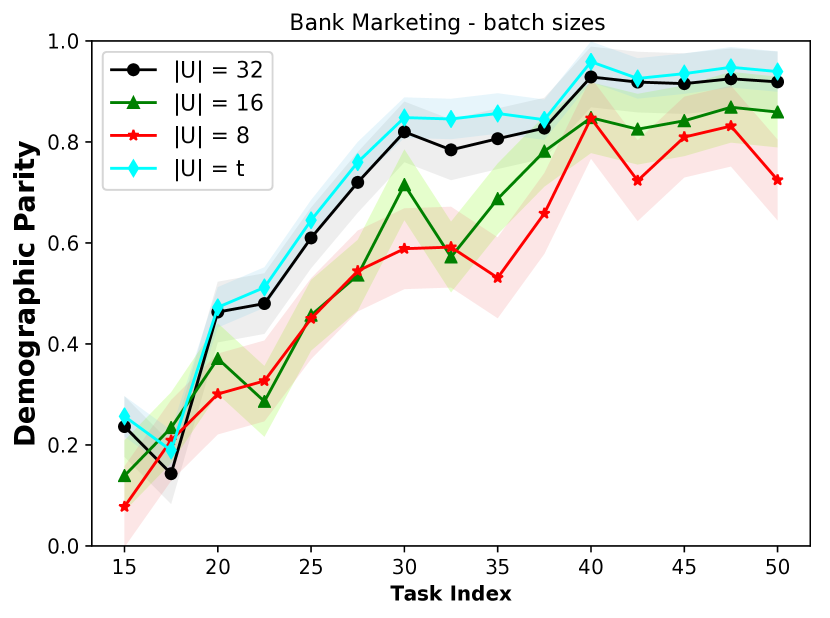
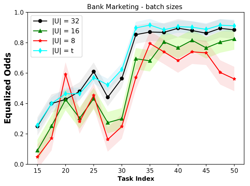
In order to reduce computational time in Algorithm 1, in stead of using all tasks, we approximate the results in practice with a fixed size of task buffer $\mathcal{U}$. In other words, at each round, we add the new task to $\mathcal{U}$ if $t\leq|\mathcal{U}|$. However, when $t>|\mathcal{U}|$, we stochastically sample a batch of tasks from seen tasks. Figure 6 represents results based on the Bank dataset with various batch sizes. Our empirical results indicate that although better performance is able to achieved with higher batch size, on the contrary more expensive the experiments will be.

Figure 6. FFML performance across various batch sizes.

More ablation study results on Adult and Crime datasets are given in Figure 7.

Figure 7. Ablation study of FFML on Adult and Crime datasets.

References

- (1)
- Bechavod et al. (2019) Yahav Bechavod, Katrina Ligett, Aaron Roth, Bo Waggoner, and Zhiwei Wu. 2019. Equal Opportunity in Online Classification with Partial Feedback. NeurIPS (02 2019).
- Calders et al. (2009) Toon Calders, Faisal Kamiran, and Mykola Pechenizkiy. 2009. Building Classifiers with Independency Constraints. In 2009 IEEE International Conference on Data Mining Workshops. 13–18. https://doi.org/10.1109/ICDMW.2009.83
- Cesa-Bianchi and Lugosi (2006) Nicolò Cesa-Bianchi and Gábor Lugosi. 2006. Prediction, Learning, and Games. Cambridge University Press (2006).
- Dwork et al. (2011) Cynthia Dwork, Moritz Hardt, Toniann Pitassi, Omer Reingold, and Rich Zemel. 2011. Fairness Through Awareness. CoRR (2011).
- Finn et al. (2017) Chelsea Finn, Pieter Abbeel, and Sergey Levine. 2017. Model-Agnostic Meta-Learning for Fast Adaptation of Deep Networks. ICML (2017).
- Finn et al. (2019) Chelsea Finn, Aravind Rajeswaran, Sham Kakade, and Sergey Levine. 2019. Online Meta-Learning. ICML (2019).
- Finn et al. (2018) Chelsea Finn, Kelvin Xu, and Sergey Levine. 2018. Probabilistic model-agnostic meta-learning. In NeurIPS. 9516–9527.
- Gillen et al. (2018) Stephen Gillen, Christopher Jung, Michael Kearns, and Aaron Roth. 2018. Online Learning with an Unknown Fairness Metric. NeurIPS (2018).
- Hannan (1957) James Hannan. 1957. Approximation to bayes risk in repeated play. Contributions to the Theory of Games (1957).
- Hardt et al. (2016) Moritz Hardt, Eric Price, and Nathan Srebro. 2016. Equality of opportunity in supervised learning. NeurIPS (2016).
- Hoi et al. (2018) Steven Hoi, Doyen Sahoo, Jing Lu, and Peilin Zhao. 2018. Online Learning: A Comprehensive Survey. arXiv:1802.02871 [cs.LG] (02 2018).
- Jenatton et al. (2016) Rodolphe Jenatton, Jim Huang, and Cedric Archambeau. 2016. Adaptive Algorithms for Online Convex Optimization with Long-term Constraints. ICML (2016).
- Kohavi and Becker (1994) Ronny Kohavi and Barry Becker. 1994. UCI Machine Learning Repository. (1994).
- Lahoti et al. (2019) Preethi Lahoti, Gerhard Weikum, and Krishna Gummadi. 2019. iFair: Learning Individually Fair Data Representations for Algorithmic Decision Making. ICDE.
- Lichman (2013) Moshe Lichman. 2013. UCI Machine Learning Repository. (2013).
- Lohaus et al. (2020) Michael Lohaus, Michael Perrot, and Ulrike Von Luxburg. 2020. Too Relaxed to Be Fair. In ICML.
- Mahdavi et al. (2012) Mehrdad Mahdavi, Rong Jin, and Tianbao Yang. 2012. Trading regret for efficiency: online convex optimization with long term constraints. JMLR (2012).
- Miller (2020) Jennifer Miller. 2020. Is an Algorithm Less Racist Than a Loan Officer? www.nytimes.com/2020/09/18/business/digital-mortgages.html (2020).
- Moro et al. (2014) Sérgio Moro, Paulo Cortez, and Paulo Rita. 2014. A data-driven approach to predict the success of bank telemarketing. DSS (2014).
- Nagabandi et al. (2019) Anusha Nagabandi, Chelsea Finn, and Sergey Levine. 2019. Deep Online Learning via Meta-Learning: Continual Adaptation for Model-Based RL. ICLR (2019).
- Patil et al. (2020) Vishakha Patil, Ganesh Ghalme, Vineet Nair, and Yadati Narahari. 2020. Achieving Fairness in the Stochastic Multi-Armed Bandit Problem. AAAI (2020).
- Rusu et al. (2019) Andrei A Rusu, Dushyant Rao, Jakub Sygnowski, Oriol Vinyals, Razvan Pascanu, Simon Osindero, and Raia Hadsell. 2019. Meta-learning with latent embedding optimization. ICLR (2019).
- Schmidhuber (1987) Jurgen Schmidhuber. 1987. Evolutionary Principles in Self-Referential Learning. (1987).
- Slack et al. (2020) Dylan Slack, Sorelle Friedler, and Emile Givental. 2020. Fairness Warnings and Fair-MAML: Learning Fairly with Minimal Data. ACM FAccT (2020).
- Wang et al. (2021) Zhuoyi Wang, Yuqiao Chen, Chen Zhao, Yu Lin, Xujiang Zhao, Hemeng Tao, Yigong Wang, and Latifur Khan. 2021. CLEAR: Contrastive-Prototype Learning with Drift Estimation for Resource Constrained Stream Mining. In WWW.
- Yao et al. (2020) Huaxiu Yao, Yingbo Zhou, Mehrdad Mahdavi, Zhenhui Li, Richard Socher, and Caiming Xiong. 2020. Online Structured Meta-learning. NeurIPS (2020).
- Yu et al. (2017) Hao Yu, Michael J. Neely, and Xiaohan Wei. 2017. Online Convex Optimization with Stochastic Constraints. In NeurIPS.
- Yuan and Lamperski (2018) Jianjun Yuan and Andrew Lamperski. 2018. Online convex optimization for cumulative constraints. NeurIPS (2018).
- Zafar et al. (2017) Muhammad Bilal Zafar, Isabel Valera, Manuel Gomez Rodriguez, and Krishna P. Gummadi. 2017. Fairness Constraints: Mechanisms for Fair Classification. AISTATS (2017).
- Zemel et al. (2013) Richard Zemel, Yu Wu, Kevin Swersky, Toniann Pitassi, and Cynthia Dwork. 2013. Learning Fair Representations. ICML (2013).
- Zhao and Chen (2019) Chen Zhao and Feng Chen. 2019. Rank-Based Multi-task Learning For Fair Regression. IEEE International Conference on Data Mining (ICDM) (2019).
- Zhao and Chen (2020) Chen Zhao and Feng Chen. 2020. Unfairness Discovery and Prevention For Few-Shot Regression. ICKG (2020).
- Zhao et al. (2020a) Chen Zhao, Feng Chen, Zhuoyi Wang, and Latifur Khan. 2020a. A Primal-Dual Subgradient Approach for Fair Meta Learning. In ICDM.
- Zhao et al. (2020b) Chen Zhao, Changbin Li, Jincheng Li, and Feng Chen. 2020b. Fair Meta-Learning For Few-Shot Classification. ICKG (2020).