Technical Report: Using Static Analysis to Compute Benefit of Tolerating Consistency Violation Faults
Abstract.
Synchronization is the Achilles heel of concurrent programs. Synchronization requirement is often used to ensure that the execution of the concurrent program can be serialized. Without synchronization requirement, a program suffers from consistency violations. Recently, it was shown that if programs are designed to tolerate such consistency violation faults (cvfs) then one can obtain substantial performance gain. Previous efforts to analyze the effect of cvf-tolerance are limited to run-time analysis of the program to determine if tolerating cvfs can improve the performance. Such run-time analysis is very expensive and provides limited insight.
In this work, we consider the question, ‘Can static analysis of the program predict the benefit of cvf-tolerance?’ We find that the answer to this question is affirmative. Specifically, we use static analysis to evaluate the cost of a cvf and demonstrate that it can be used to predict the benefit of cvf-tolerance. We also find that when faced with a large state space, partial analysis of the state space (via sampling) also provides the required information to predict the benefit of cvf-tolerance. Furthermore, we observe that the cvf-cost distribution is exponential in nature, i.e., the probability that a cvf has a cost of is , where and are constants , i.e., most cvfs cause no/low perturbation whereas a small number of cvfs cause a large perturbation. This opens up new aveneus to evaluate the benefit of cvf-tolerance.
1. Introduction
As we see an end to Moore’s law, parallel/concurrent computing has become essential to solving problems efficiently because now, instead of increasing the power of processors, technology is witnessing integration of multiple processors on the same chip. While an individual processor becomes faster over time, this increased speedup is dwarfed by the increase in the number of processors/cores. To fairly utilize such an architecture now, mutiprocess computing is implemented. In such implementations, the task is to solve the same problem collectively; processes share data and communicate with each other to achieve so. Such implementations is done in two ways based on how far processors are placed from each other. If the processors are placed on a single chip, then the processes communicate with one another under the shared memory model. If, on the other hand, the processors are placed remotely from each other, then the processes communicate with one another under the message passing model.
In multiprocessor computing, it is always desired that the system implemented is execution faithful, that is the execution of the program appears as if it was executed by a uniprocess program. To achieve this, programs are often implemented under synchronization constraints, e.g., locks, locksteps, and semaphores. If synchronization requirements are violated then a process would read inconsistent values of variables.
The authors of (NKD2019ICDCN.short, ) introduced the notion of consistency violation faults (cvfs) to model such improper simultaneous access to shared data. For example, in case of the vertex cover problem, simultaneous updates may cause two adjacent nodes to enter the vertex cover simultaneously. The cvfs could cause the program to diverge from its goal state (e.g., a minimal vertex cover). However, the underlying program is able to handle such inconsistency to reach the goal state. In (NK2020SRDS.short, ), authors have considered various problems including token ring, graph coloring, and maximal matching. Here, it was observed that there is a substantial benefit in permitting cvfs and tolerating them rather than eliminating them using synchronization approaches such as local mutual exclusion.
Now after establishing that tolerating cvfs is beneficial, especially in terms of convergence time, it is desired that we are able to predict the overheads involved in tolerating the cvfs, especially when the problem size increases. Currently, the only known approach to make such predictions is experimental analysis where you consider the execution of the program without cvfs (i.e., with suitable synchronization) and with cvfs (where cvfs are permitted). It is highly desirable that we can predict the expected improvement from cvf tolerance without such experimental analysis which is both time consuming and does not allow one to predict the expected benefit under different execution conditions (e.g., level of concurrency).
One way to ameliorate this is to predict the expected performance gain via static analysis. If feasible, this would indicate that we can analyze the given program once so we can identify the expected benefit of the given program by simply analyzing its code rather than by run-time analysis. In turn, this would allow us to predict the expected performance gain under different levels of concurrency and different memory models.
With this motivation, the first goal of this work is to understand if static analysis of programs can provide sufficient information about the ability to gain performance by tolerating cvfs instead of eliminating them.
It is also important to address known limitations of static analysis, viz. state space explosion. Specifically, as problem size increases, the size of the state space increases exponentially thereby making static analysis difficult/impossible. The way to get around this is to generalize from small programs and to do sampling of state space. If successful, we can get an understanding of how cvf-tolerance will improve performance of large programs using small programs. Or, we can only partially analyze the state space to identify expected performance gain from partial analysis of the state space.
With this motivation, the second goal of this work is to understand if partial analysis of state space provides sufficient information to gauge the performance gain provided by full static analysis. Or, if the performance gain of small programs can be generalized to the corresponding large programs.
The third goal of this paper is to determine how the cost of cvfs varies in different programs. Specifically, if we can empirically determine the distribution cost of cvfs then it would allow us to benefit from existing tools for statistical analysis.
Based on the above discussion, we focus on static analysis of three programs, for distributed token ring, graph coloring and matching on message passing model. These problems were chosen because they are self-stabilizing (EDW426, ) which implies that they are able to tolerate cvfs (cf. Section 3 for justification). For these programs, we analyze their state space and define a rank of each state which captures how long it will take for the program to reach the goal state (e.g., valid coloring) from that state. Then, we can define the benefit of a regular program transition (change in rank due to a program transition) and the cost of a cvf (change in rank by a cvf). Subsequently, we analyze how the benefit of program and cvf transitions varies across programs and input sizes.
The contributions of the paper are as follows:
-
•
Regarding our first goal, we show that static analysis, indeed, provides sufficient information about expected speedup.
-
•
Regarding our second goal, we show that partial analysis of the state space does provide sufficient information about the performance in the presence of cvfs. In turn, this indicates that one can generalize results from smaller programs to larger programs (with more number of nodes/edges).
-
•
Regarding the third goal, we find that the cost distribution of cvfs is exponential in nature. In other words, the probability that a given cvf perturbs the rank by is where and are constants. This means that most cvfs have low cost whereas a few cvfs have a large cost. In turn, this implies that existing statistical techniques can provide information about performance gain in the presence of cvfs.
-
•
Additionally, we analyze the cost distribution of cvfs in these programs. We compute the trend of the same program; this trend predicts the cost distribution of cvfs as the problem size increases.
-
•
By focusing on the average benefit of program transitions and cvfs (under the assumption that they are equally likely), we compute which denotes the average number of program transitions needed to undo the effect of a cvf. We compute for our case studies using full analysis (where we construct the entire state space to determine ranks of each states) and partial analysis (where rank computation is done by sampling). We consider average-rank and max-rank. We find that partial analysis provides results that are close to the full analysis thereby demonstrating that we can consider only sampling based approach when the state space is large.
Organization of the paper. The rest of the paper is organized as follows. In Section 2, we define the computational model. We introduce cvfs in Section 3. Section 4 presents our approach for computing the cost of cvfs. Section 5 identifies the cost distribution of cvfs. In Section 6, we compute the relative cost of cvfs compared to the benefit of program transitions. We evaluate the steps required for convergence in the presence of cvfs in Section 7. In Section 8, we interpret these results and discuss their implications for executing concurrent algorithms. Section 9 discusses related work. Finally, Section 10 provides conclusion.
2. Modeling Parallel/Concurrent Programs
A distributed/parallel/concurrent program consists of a set of processes (ag94, ). Each process has a set of neighboring processes, denoted as . Each process is associated with a set of variables and a set of actions. Each action of process is of the form , where is a Boolean expression involving variables of and the variables of its neighbors , and is the statement that updates the variables of .
The state of a process is obtained by assigning values to all the variables of from their respective domains. Variables of program are the union of the variables of its processes. A state of program is obtained by assigning values to all the variables of . The state space of program is the set of all possible states of .
We say that an action of some process is enabled in a state iff evaluates to true in . Transitions of process in program is the set and is obtained from by executing one of the enabled actions of . The transition of program is the union of the transitions of all its processes.
A computation of program is of the form , where is a state of the program and is a transition of . For the sake of simplicity, we assume that each state has an outgoing transition, i.e., for any state , there exists a state such that is a transition of . To achieve this, if no action in any process is enabled in state then we add as a transition of .
A state predicate is a Boolean expression involving variables of . We also overload to denote a subset of the state space where predicate is true. In other words, we use the Boolean expression and the set of all states where the value is interchangeably.
3. Consistency Violation Faults.
The program computation model assumes that each action execution is atomic. Thus, a consistency violation happens when a process reads old values of one or more other processes, and performs an execution based on those values. Reading old values may cause process to incorrectly go from state to where is not a transition of . We denote such execution as a consistency violation fault (cvf).
We illustrate cvfs with an example of a simple graph coloring program where a node changes its color to another available color if it finds that its color matches with that of its neighbor (see Appendix A for detailed descriptions of the program). Consider the state of this program where processes and are neighbors. If process (respectively ) executes then the resulting state would be (respectively, ). On the other hand, if both processes execute simultaneously then the resulting state would be . Clearly, this is undesirable and the colors may remain invalid forever.
This problem can be addressed via local mutual exclusion (10.1007/3-540-40026-5_15, ; KY2002SRDS, ; NA02JPDC, ; dima, ) that guarantees that two neighboring processes do not execute at the same time. Clearly, local mutual exclusion introduces an overhead as it requires extra work to coordinate among the processes and block the waiting processes.
While the above example is focused on simultaneous execution of the program actions, such execution is an instance of consistency violation faults where the process executing the action reads an incorrect value for one of its neighbors’ variables. In this example, transition from to can be thought of as a transition from to by process and then transition from to by process where it reads an old value () of . This latter transition is an instance of cvf.
It follows that consistency violation faults associated with program are subset of , where is the state space of . Hence, we can extend the definition of a computation as follows.
Computation in the presence of cvfs. A sequence is a computation of program in the presence of iff for each , is a transition of or is in . (Note that are not required to be terminating, i.e. the number of cvfs can be infinite.)
Permitting and tolerating cvfs differs from traditional approaches of concurrent computing where the goal is to keep the state of the program to be correct by ensuring that action execution can always be viewed to be atomic. As we have seen, cvfs have the potential to perturb the program computation from its goal states. Our goal in this paper is to analyze the properties of such cvf transitions. We study cvfs in the graph coloring problem, token ring problem and maximal matching problem. Specifically, we study the distribution of the cost of cvfs in these programs. We also evaluate the cost of these cvfs while analyzing the execution time for these programs.
3.1. Self-stabilization and cvfs
In this section, we review the definition of self-stabilizing programs and relate it to cvfs. A stabilizing program is guaranteed to recover from an arbitrary state to its legitimate states. Specifically,
Let be a program and be a state predicate of . We say that is self-stabilizing (respectively, stabilizing) with invariant iff
-
•
Any program computation includes a state where is true. In other words, for any computation , there exists a state such that
-
•
If is a transition of and then .
In other words, starting from an arbitrary state, a stabilizing program reaches a state in and stays there forever. If is stabilizing to invariant then is the legitimate states of program .
We observe that a stabilizing program naturally tolerates (finite number of) cvfs. In other words,
Observation 1.
Let be a stabilizing program with invariant . Let be a computation of in the presence of cvfs. If the number of occurrences of cvfs is finite in then will reach a state in and stay there forever.
This follows from the fact that if cvfs are finite then once they are done, the program is guaranteed to recover due to the property of stabilization. We focus on analyzing probabilistic stabilization (Herman90IPL, ) of stabilizing programs when cvfs are not finite.
4. Modeling Cost of cvfs
While determining the cvfs for a given process/program is potentially a challenging task, we can see that cvfs at , namely is a subset of , where
{ is obtained by changing variables of in }
Similar to transitions of a program, we can define cvfs for a program. In other words, (, respectively) for program is the union of () where is a process in .
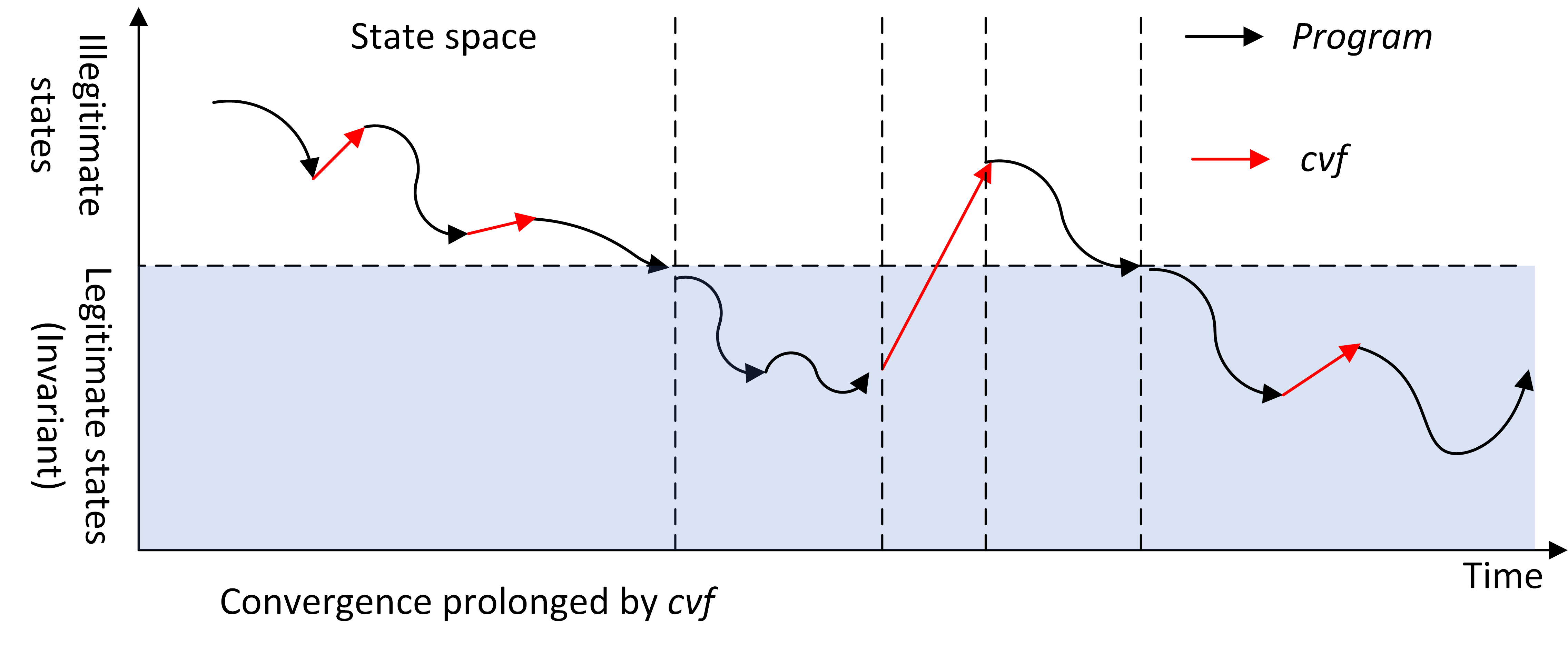
Let be a computation of program in the presence of . Thus, we can view the execution of a stabilizing program as shown in Figure 1 where the rank of each state is depicted by how far the state is from a legitimate state (a state in the invariant). Examples of such rank functions include (minimum, average, or maximum) steps/time required to reach a state in . Specifically, the rank of states in is and a sufficiently long program computation decreases the rank of the program state.
 \Description
find me
Note that execution of cvfs may cause the rank value to increase thereby increasing steps for recovery (or preventing the recovery). However, the time required to execute one step is lower if cvfs are permitted to occur, as there would be no need to add any synchronization to ensure atomicity of action execution.
To guarantee convergence in spite of cvfs, we need to ensure that the rank decreases in a computation over time even if it does not decrease in every step. In other words, consider a sufficiently long computation in the presence of cvfs: , where all states in the computation are outside legitimate states. In this case, we need to ensure that . If this is assured then eventually the program will reach a state whose rank is , thereby guaranteeing the recovery/valid termination of the program. Additionally, cvfs are not malicious in nature since they are caused when a node reads an older value for one of its neighbors. In other words, cvfs are random and unintentional. Hence, we can focus on the average effect of cvf (using statistical analysis) instead of the worst-case effect. With this motivation, the goal of the paper is to study rank changes by program and cvf transitions.
Average rank change by cvfs. Since identifying precise cvf transitions for a given program is a challenging task, we can approximate it with . We have various choices for defining the rank of a state. For example, we could use the average/minimum/maximum number of transitions required to reach a legitimate state. One observation in this context is that the increase (respectively, decrease) in the rank from to is the same as the decrease (respectively, increase) in the rank from to . Moreover, if then . Thus, if we average the change in rank of all transitions in then the average is .
Observation 2.
The average change in rank by transitions in is .
What the above result shows is interesting and misleading. It is interesting because it shows that if all cvfs were equally likely then the overall benefit and loss caused by cvfs would be . At the same time, this result is misleading because the actual cvfs that could occur are a subset of those in . Since our goal is to determine the frequency of cvfs under which convergence property is not affected, we only focus on cvfs that increase the rank.
Defining . We also introduce the notion of . This is also a superset of actual cvfs that could occur in the program but a subset of . To understand the notion of , observe that, in action , the process may read arbitrary values of its neighbors but it will change its state by executing . For example, if was of the form where is a local variable of the process then a cvf cannot perturb the program from a state where to (note that this perturbation is allowed in ). Since cvfs of a given program can be very difficult to compute, we use as an approximation of cvfs. Note that the average rank of transitions in need not be . Furthermore, we only consider those cvfs that increase the rank.
5. Computing the Benefit of Program Transitions and Cost of cvfs
As discussed earlier, to compute the benefit of a program transition (respectively, cost of cvf) , we need to find the ranks of and and the benefit of the program transition (respectively, cost of cvf) is . There are several choices to define the rank subject to the constraint that the rank of legitimate states should be and the rank of illegitimate states should be positive. We consider two options
-
•
max-rank, where is the length of the maximum path from to reach a legitimate state.
-
•
average-rank, where is the average length of all the paths from to reach a state in the invariant.
Note that for a stabilizing program, the rank will always be finite since each computation is eventually guaranteed to reach the invariant. Furthermore, we can utilize existing algorithms to compute max-rank and average-rank. Outline of these algorithms is in Appendix B. Once the rank of every state is computed, we compute the benefit of a program transition to be . Then, we compute the average benefit of all program transitions. For cvfs, as discussed above, we only consider cvfs that disturb the convergence, i.e where . We compute the average cost of those cvfs.
5.1. Case Studies
We consider three case studies: token ring program by Dijkstra (EDW426, ), Graph Coloring program by Gradinariu and Tixeuil (GT2000OPODIS.short, ) and maximal matching program by Manne et al. (MMPT2009TCS.short, ). Since the description of the algorithms is not critical for the subsequent discussion, for reasons of space, we describe them in Appendix. The only property we use of these algorithms is that they are stabilizing.
5.2. Program and Cvf distribution
In this section, we evaluate the benefit and the cost of program and cvf transitions for the three case studies. Figure 2 shows the probability distribution of the rank effect for program and cvf transitions using max-rank and average-rank.
As an illustration of these results in Figure 2b, we consider the token ring program with 9 processes. We find that 9% of the cvf transitions have no effect on the rank. 27% of cvf transitions change the rank by at most 1, i.e., they undo the effect of at most one program transition. 50% of the cvf transitions change the rank by at most 5. However, 0.6% of cvfs change the rank by 50 or more, i.e., to undo their effect, 50 or more program transitions are needed.
Yet another observation from Figure 2 is that with max-rank, the rank effect of program transitions is always negative whereas with average-rank, the effect of program transitions is occasionally positive. (This is expected since average-rank may not decrease with every program transition.)
From Figure 2, we find that the distribution of cvfs is exponential in nature in that the fraction of cvfs with cost decreases exponentially with . The approximation curves (straight lines) are obtained in these figures as follows. We logscaled the fraction (probability) of the cvfs observed against their rank effect. The continuous blue and red curves are the curves of cvf count and program transition count respectively. The dotted blue and red curves are the approximation curves of blue and red continuous curves respectively, modelled as a straight line. The approximation for cvfs is done only for the positive domain, that is, only where the positive rank effect is observed. The proximity between the continuous curves and the respective observed curves shows that there is in fact an exponential decrease in the number (fraction) of cvfs with increase in rank effect.
| #nodes | Avg rank |
|---|---|
| 5 | |
| 6 | |
| 7 | |
| 8 | |
| 9 |
| #nodes | Avg rank |
|---|---|
| 5 | |
| 6 | |
| 7 |
| #nodes | Avg rank |
|---|---|
| 4 | |
| 5 | |
| 6 | |
| 7 | |
| 8 | |
| 9 | |
| 10 | |
| 11 | |
| 12 | |
| 13 | |
| 14 |
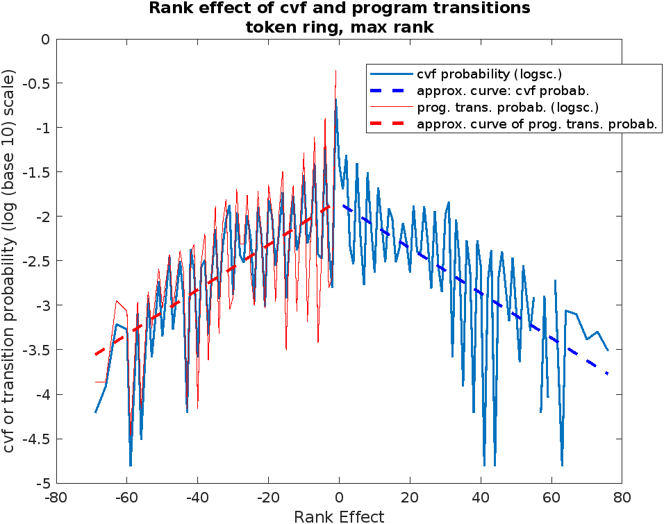
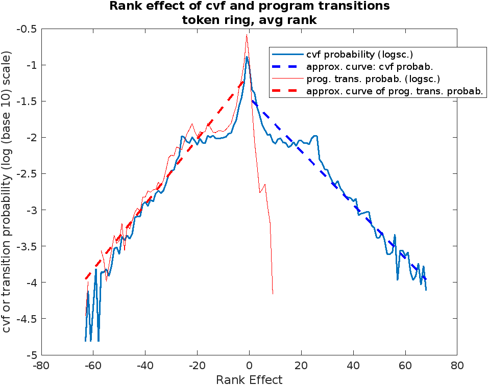
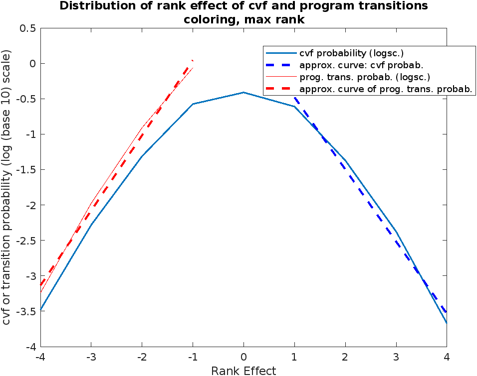

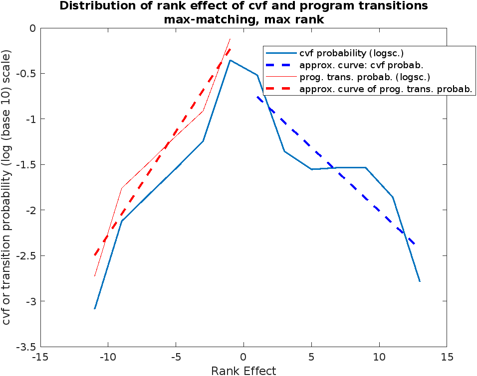
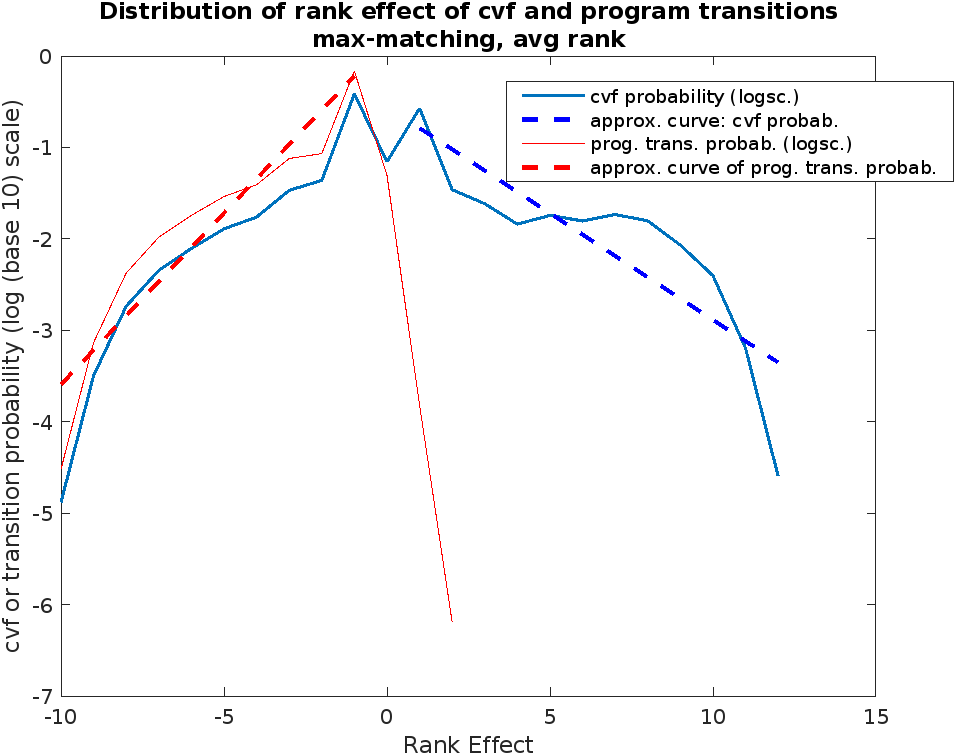
We consider a similar analysis for other sizes of the input programs as well. For the token ring program, we identify the distribution of the program and cvf transitions in Table 3. From this figure, we observe that the slope of the approximation curve strictly decreases. However, we are not able to observe the same for other programs (coloring (Table 1) and maximal matching (Table 2)).
6. Analyzing Relative Cost of cvfs with respect to Program Transitions
As discussed in Section 5, each program state has a rank (either max-rank or average-rank). The rank effect of a state change (which could be a program transition or a cvf) is the difference .
While Section 5 focuses on the distribution of individual cvf and program transitions, in this section, we consider the average effect of program and cvf transitions. To this end, in Section 6.1, we define the relative effect between program and cvf transitions. We describe full and partial analysis in Section 6.2. We analyze the case studies under these two analysis paradigms. In Section 6.3, we present the observations that we obtained from the experiments. We analyze these observations and derive approximation curves of cvfs of positive rank effect based on the observations.
6.1. Defining
Observe that if is a program transition and then and the rank effect is 0. Hence for a given program, we evaluate the average of the rank effects of all program transitions that originate outside the invariant (i.e. ). Note that this value, denoted as is negative since program transitions reduce the rank overall. Similarly, we compute , the average rank effects of cvfs that begin outside the invariant. As mentioned in Section 3, we only focus on cvf transitions that increase the rank thereby making the analysis conservative in nature. Therefore, . The relative recovery cost of cvfs is defined as
The relative recovery cost measures how many program transitions, on average, are needed to equalize the perturbation effect of a cvf.
We evaluate the cost of cvfs and the benefits of program transitions on the same three self-stabilizing programs. For graph coloring and maximal matching, we used three types of input graph (topology) in our evaluation: ring, power-law graph, and random regular graph. In a power-law graph, node degrees (number of process’ neighbors) follow the power-law distribution and nodes form clusters within the graph. In a random regular graph, nodes have the same degree and are randomly connected. Ring is the special case of random regular graph where every node has degree 2. We used the tool networkx (networkx.duong, ) to generate those graphs.
6.2. Full and Partial Analysis
For a given case study program, we construct its entire state space and then for each state, we compute its average-rank and max-rank. For each program transition where , we compute its rank effect. Then, is the average of those rank effects. Similarly, we obtain as the average of the rank effects of all and and . As anticipated, this approach of full analysis suffers from the state space explosion problem. For example, full analysis of the token ring program with 15 processes easily exhausts 170 GB of memory. Hence, we also consider partial analysis where we compute the ranks of a number of random states without constructing the whole state space. Suppose is a randomly chosen state, we probe a pre-determined number of random paths from to the program’s invariant. The maximum and average length of these selected paths is the approximation of and , respectively. Subsequently, given the rank of two states and obtained in this way, the rank effect of a program transition (or cvf) is the difference of the ranks of and .
6.3. Computing
Analysis with max-rank and average-rank. From Figures 3 and 4, we observe that the cvf relative recovery cost does not significantly differ between max-rank and average-rank in full analysis. In other words, when we utilize full analysis, the number of program transitions required to neutralize a cvf remains the same whether we use max-rank or average-rank.
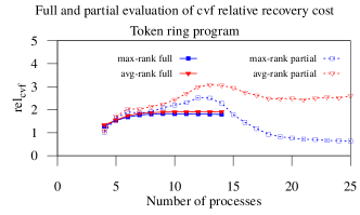
Partial Analysis vs Full Analysis. Figures 3 and 4 also consider the analysis via partial analysis and full analysis. When full analysis is feasible, we conducted both full and partial analysis. Otherwise, we only considered partial analysis. When both are possible, they are consistent with each other. This indicates that partial analysis provides reasonably good estimates of full analysis. We also find that partial analysis via average-rank is more stable and follows the trend of full analysis better than the analysis of max-rank. This is expected because the sampling method generally provides a good estimate of the average value but not the extremum. This is beneficial since the average-case cost of cvfs is more relevant regarding the convergence to legitimate states. The results also imply that we can get a good estimate of when the state space is large.
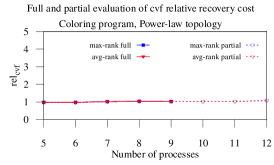
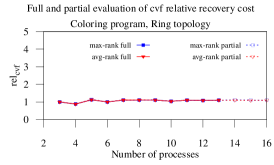
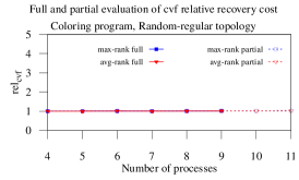
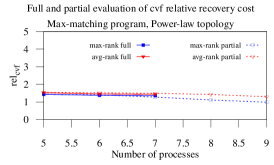
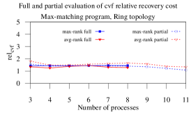
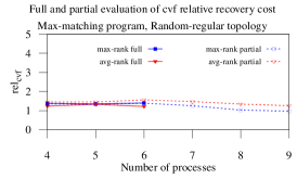
Observations about values of . Although the specific pattern and values of depend on given case study, we observe that the value of is small (roughly 2-4) indicating that the stabilization property is likely to be (probabilistically) preserved even if cvfs are frequent and only a small number (2-4) of program transitions execute between cvfs. Also, the value of does not vary significantly with the number of processes indicating that analysis of a problem with a small number of processes could generalize to a large number of processes.
7. Performance Analysis in the Presence of cvfs
In this section, we validate the observations about to determine the ability of a program to converge in the presence of cvfs. If , this indicates that a cvf undoes the progress achieved via 3 program transitions. Hence, if more than 3 program transitions are executed between cvfs, it is anticipated that the recovery to legitimate states would still occur. Of course, if the number of program transitions between cvfs is just above 3 then there may be a substantial increase in the number of steps required for convergence. We evaluate this hypothesis with simulations of the given case study programs in the presence of cvfs.
We choose simulations to validate the hypothesis because simulations allow us to control the rate of cvfs. By contrast, in an actual experiment on real networked systems, we cannot easily change the rate of cvfs since we cannot control when two neighboring processes access the same data item simultaneously . Furthermore, in an actual system, methods used to detect cvfs interfere with the actual computation. In simulations, we introduce the parameter cvf_interval to denote the average number of program transitions between cvfs. For example, means (on average) 4 program transitions execute between consecutive cvfs.
We conduct our simulations as follows: We randomly select an initial state, say , and emulate a computation of the given program from that initial state. In order to emulate such a computation, in each iteration, we execute a random enabled action. Furthermore, in each iteration, we randomly choose a process and perturb the state of that process in such a way that mimics the effect of a cvf. The parameter cvf_interval determines how frequently cvfs are introduced. We terminate the execution when the program state is legitimate (inside the invariant) or when the number of iterations exceeds a threshold. In the latter case, we treat it as if the program has failed to converge in the presence of cvfs. Let convergence_steps denote the number of iterations by the time of termination. For each initial state (), we consider five computations and take the average of convergence_steps. Subsequently, for the same initial state, we compute convergence_steps for different values of cvf_interval.
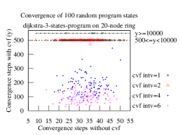
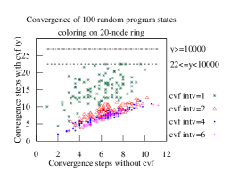
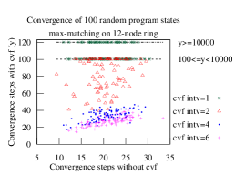
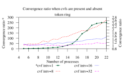
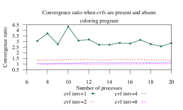
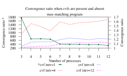
We present the data from our simulations in Figure 5 as a scatter plot and in Figure 6 as the relative increase in the number of steps for convergence due to cvfs. In Figure 5, each point is the simulation results of a given program for an initial state with a specific cvf_interval value. A point with coordinate indicates that for the initial state considered, it took on average steps ( steps, respectively) for the program to converge in the absence (in the presence, respectively) of cvfs with the given value of cvf_interval. To present the data in an easy-to-read fashion, we remove certain details when coordinate is large. For example, in Figure 5a, we group the points when coordinate is between 500 – 10000 (threshold) to indicate that convergence was achieved but it took too long.
Figure 6 presents the simulation data to compare the number of steps for convergence in the absence of cvfs and in the presence of cvfs. If cvf_interval is small then the number of steps to converge could be very large (or infinite). This is observed in Figure 6a where the number of steps increases by a factor of or more if . However, if , the number of steps for convergence in the presence of cvfs is about times more than the number of steps in the absence of cvfs. This is consistent with the analysis in Figure 3 for the token ring program where the ratio is about 3. That means that a cvf negates the benefit of (approximately) 3 program transitions. Hence, the benefit of 8 program transitions and 1 cvf is (approximately) the same as 5 program transitions, thereby increasing the number of steps to be (i.e., ) times.
Figure 6b analyzes the coloring program. Here, from Figure 4, the program is expected to converge even if a cvf occurs between two consecutive program transitions. Figure 6b confirms this anticipation and finds that the increase in the number of steps is approximately 3 times if . If cvf frequency is reduced then the increase in the number of steps drops quickly. For example, if then there is virtually no increase in the number of steps for convergence. Figure 6c considers the same question for the maximum match problem. As expected, when cvfs are too frequent (), the increased steps is very high. But when cvf frequency is reduced (), the increase is only .
Note that it is anticipated that convergence_steps will increase in the presence of cvfs. However, each step is expected to be faster, as processes do not need to synchronize with each other.
8. Interpreting the Results of Case Studies and Their Implications
As discussed in the Introduction, existing approaches for concurrent computing focus on ensuring that the program state is always consistent. In other words, these approaches rely on preventing cvfs. However, to use these approaches in practice, it is necessary for coordination among threads in the given program. By contrast, permitting and tolerating cvfs allows one to eliminate synchronization between threads as each thread could work independently.
8.1. Number of Steps vs Time
In this work, we intentionally focused on number of steps required for convergence instead of time. Note that with cvf-tolerance, we can run the program without the necessary coordination/synchronization. Hence, we expect that if the program is run with concurrent threads, we can get a speedup of (subject to suitable load balancing). By contrast, without cvf-tolerance, we will need to ensure that execution of each action is atomic and therefore will suffer from large overhead of lock/unlock.
Additionally, when comparing cvf-prevention and cvf-tolerance, consider the case where cvf-prevention is implemented using local mutual exclusion. Specifically. if node is executing at a given time none of its neighbors can execute at that time. Thus, if we have the underlying graph to be a 2-dimensional grid then at most half of the nodes can execute at a time. This means that as long as the number of steps does not increase 2-fold, cvf-tolerance is expected to provide a benefit over cvf-prevention. Taking this further, one would expect that at most nodes can execute at a given time where is the independence number (size of the maximum independent set) of the communication network among the processes. Hence, as long as the number of steps does not increase by a factor of , cvf-tolerance is expected to be better.
When we eliminate cvfs, an action at node would require that first lock the relevant data then execute the action and then release the lock. There are two types of overheads in this scheme. First, there is an overhead for obtaining and releasing the locks even if there is no contention. Second, there is the required waiting if the locks are not available when requested. To estimate these overheads, we considered the execution of graph coloring program (GT2000OPODIS.short, ) using only one thread- with and without the necessary locks. Since our goal was to evaluate the overhead, we ran the program with 1000 steps. Since there is only one thread, the overhead is only for acquiring locks (as there is no contention). Even under these circumstances, the time of execution was more than 2-fold when locks were acquired before every step. The actual overhead would be higher when we account for contention and where some threads need to wait on acquiring the locks.
Our results from Section 7 show that in most cases, the increased number of steps is very small (typically, less than 20%). Thus, the increased number of steps would not significantly affect the performance when compared with the approach of cvf-prevention.
We anticipate that a slight variation between the overhead (e.g., 10% increased steps vs 20% increased steps) would not substantially affect the performance. By contrast, in a handful of cases where the rate of cvfs is very high (e.g., token ring program with one cvf between two program actions), cvf-prevention is preferable to cvf-tolerance.
8.2. Implication for Stabilizing Programs
Our focus in this paper was in stabilizing programs that, by definition, tolerate cvfs. Specifically, if the number of cvfs is finite, the program is (deterministically) guaranteed to converge. And, if the frequency of cvfs is small, the program is guaranteed to converge probabilistically.
When we view tolerating cvfs through the lens of algorithms such as matching and coloring, we note that these algorithms are silently stabilizing . In other words, once the program reaches the state where valid matching or coloring is found, there is no need to execute any actions further. Such programs benefit the most from cvf-tolerance, as they can continue to run until they reach a legitimate state. At this point, cvfs (which are caused by reading old values of variables) have no effect, as the program state remains unchanged forever.
Programs such as token rings are not terminating, i.e., they continue to execute even after they reach legitimate states. If cvfs occur when the program is in a legitimate state, it is possible that the cvfs may cause the resulting state to be illegitimate. If this happens, the program will still return to legitimate states. However, this behavior is different from the behavior of stabilizing token ring program which guarantees that once a legitimate state is reached, subsequent computation remains in legitimate states in the absence of faults. In other words, once legitimate states are reached, we should prevent cvfs rather than tolerate them. However, outside the legitimate states the program should permit and tolerate cvfs. Thus, the execution can be partitioned into two phases (1) quiescent phase where the algorithm has recovered to legitimate state(s) and no recovery actions are needed, (2) recovery phase, which is initiated by some node due to an observed inconsistency.
For any self-stabilizing algorithm, it is desirable that the time spent in the recovery phase is as minimal as possible. The results in this paper allow us to reduce the time spent in the recovery phase. The intuition of how to achieve this is as follows:
If a node enters the recovery phase, it should transition itself to quiescent phase after a certain time, say . When a node enters the quiescent phase, it should remain there for a certain duration, , to prevent constant transition from recovery to quiescent phase (and vice versa). Furthermore, in recovery phase, the execution should permit and tolerate cvfs. By contrast, in quiescent phase, the execution should be conservative, i.e., it should eliminate cvfs. (Note that cvfs are possible even if a single node is in the recovery phase.)
Observe that as long as is large enough, recovery to legitimate states is guaranteed. Furthermore, as long as the program is in a legitimate state and each process is in the quiescent phase, the program would remain in a legitimate state. Additionally, as long as cvfs are rare, during the recovery phase, faster execution to the invariant would be possible. From the analysis, we observe that the actual perturbation caused by a cvf is typically very small, just a handful of program transitions are sufficient to neutralize its effect. In turn, this implies that the time spent by the program outside legitimate states can be reduced if the program permits cvfs when the state is perceived to be outside legitimate states and eliminates cvfs when the state is perceived to be inside legitimate states.
9. Related Work
In this work, we focused on permitting and tolerating cvfs rather than preventing them as done in most concurrent algorithms. The closest work to permitting and tolerating cvfs is that by Garg (garg20, ) on Lattice Linear Problems. A key property of these programs is that the set of reachable states form a lattice with one optimal state and it is guaranteed that in any suboptimal state, there is some node whose execution is critical. If this node executes with old information about others, it will either perform the correct action or perform no action. Thus, when this critical node executes, the program will reach closer to the optimal state. Due to the lattice structure, it is guaranteed that the program will reach the optimal state even if any number of cvfs occur. Unfortunately, the requirement of the lattice structure makes it impossible to use it in various problems where underlying state space does not form a lattice.
Stabilizing programs (EDW426, ), by contrast, tolerate cvfs if they are either terminating or infrequent. In other words, their tolerance of cvfs is less than that for lattice linear programs. However, they are applicable for a large class of problems. Stabilizing algorithms have been designed for spanning trees (ag94, ) leader election (ADDDL2017IPDPS, ), matching (IOT2019PODC, ), dominating set (KKM2017SSS, ), clustering (DBLP:journals/tcs/DattaDHLR16, ), etc.
In (NK2020SRDS.short, ), the concept of consistency violation fault was introduced as a formalization of the program perturbations that occur when local mutual exclusion is removed. While the experimental results of (NK2020SRDS.short, ) demonstrated an improvement in performance, the reasoning behind it was unclear To the best of our knowledge, this paper is the first work that formally analyzes the effect of cvfs during the recovery phase of self-stabilizing programs to show that the effect of cvfs is small and can be computed for a given program. It also shows the rate of cvfs for which overall recovery would be faster. In turn, it can assist designers to determine the best approach for reducing convergence time for a given self-stabilizing program.
10. Conclusion
Execution of concurrent program has typically relied on ensuring that the program state always remains consistent. This requirement is enforced through various mechanisms such as linearizability, local mutual exclusion, etc. Thus, even when concurrent operation is permitted, the goal is to ensure atomicity so that the operations can be ordered in some fashion.
Our focus is on an alternative approach. Specifically, we focus on permitting and tolerating consistency violation faults (cvfs) rather than eliminating them as it is done in traditional literature. There is empirical evidence that such an approach can significantly enhance the performance, if the program is designed to tolerate cvfs. However, the only evidence of this is via experimental analysis that makes it difficult to determine the expected benefit of cvf-tolerance without experimental evaluation.
In this paper, we demonstrated that the results of experimental evaluation can be predicted by static analysis of the program state space. Furthermore, even partial analysis provides sufficient details to determine if cvf-tolerance would be beneficial. Towards this end, we focused on analyzing three stabilizing programs (that naturally tolerate cvfs) to evaluate how cvfs affect them.
We analyzed the cost of cvfs in the steps required for recovery (i.e., to reach legitimate states from an arbitrary state) in these case studies. To this end, we defined the notion of average-rank and max-rank that identify how far a given state is from a legitimate state (e.g., a state with valid coloring). We evaluated the rank change by cvfs and by program transitions. We observed that the cost of cvfs follows an exponential distribution. In other words, the probability that a cvf increases the rank by is , where and are constants. This indicates that while most cvfs have a minimal cost on recovery, a few cvfs can cause a significant perturbation. We also observed that the benefit of program transition (i.e., rank change by the program transition) also follows an exponential distribution.
We also computed the relative cost of cvf when compared with program transitions. Specifically, we consider which denotes the number of program transitions that would be needed to compensate for a single cvf. Specifically, this is computed by treating as if all cvfs and program transitions are equally likely and taking the ratio of the average rank change by a cvf and the average rank change by a program transition. We compute by either full analysis of the program state space or via partial analysis. The former is more accurate but suffers from state space explosion. We find that the computation of by both analysis match when we can utilize both approaches. This indicates that partial analysis (especially with average-rank) would suffice to compute the relative effect of cvf.
We also evaluated the actual effect on recovery in the presence of cvfs and compare it to . As characterizes the number of program transitions needed to compensate the effect of a single cvf, if program transitions occur between cvfs then we expect that program transitions will not make substantial progress. On the other hand, if substantially more program transitions execute between cvfs (e.g., 2 program transitions execute between cvfs)) then the program continues to converge without a significant increase in the number of steps for convergence.
We have developed a toolset that is generic so that by only coding the specific algorithm, one can obtain the effect of cvf on that program. Specifically, our analysis of max-rank and average-rank uses program transitions as a parameter. Thus, simply specifying the new program transitions, one can analyze the effect of cvfs for the given program. We intend to provide this as a toolset for the community to use.
There are several future work in this area. One is to relate the occurrence of cvfs with the level of concurrency and the size of the input. A cvf occurs due to non-atomic execution of program actions. Thus, it is likely to increase with level of concurrency (more conflict when the number of concurrent threads increases but size of the input is kept constant) and decrease with the size of the input (less chance of a conflict if the input size is increases but the available threads are kept constant). Another future work is developing Markov chain model using the exponential nature of the rank change for program and cvf transitions. Our focus in this paper was on stabilizing programs because they are naturally cvf-tolerant and there is a vast literature that provides stabilizing algorithms. However, another future work is in developing algorithms that tolerate cvfs without being stabilizing.
We observe that for the token ring program that on a logarithmic scale, the slope of the (approximation) curve of cvfs against rank effect decreases, except for one anomaly. It means that keeps decreasing as the order of the input graph increases. We do not have the same observations for coloring and maximal matching programs. Hence, one of the future works is to study and possibly determine how the cvf distribution changes with the size of the input.
References
- (1) Overview of networkx. https://networkx.github.io/documentation/stable/. Accessed: 2021-May-20.
- (2) Altisen, K., Datta, A. K., Devismes, S., Durand, A., and Larmore, L. L. Leader election in asymmetric labeled unidirectional rings. In 2017 IEEE International Parallel and Distributed Processing Symposium, IPDPS (2017), IEEE Computer Society, pp. 182–191.
- (3) Arora, A., and Gouda, M. G. Distributed reset. IEEE Trans. Computers 43, 9 (1994), 1026–1038.
- (4) Beauquier, J., Datta, A. K., Gradinariu, M., and Magniette, F. Self-stabilizing local mutual exclusion and daemon refinement. In Distributed Computing (Berlin, Heidelberg, 2000), M. Herlihy, Ed., Springer Berlin Heidelberg, pp. 223–237.
- (5) Datta, A. K., Devismes, S., Heurtefeux, K., Larmore, L. L., and Rivierre, Y. Competitive self-stabilizing k-clustering. Theor. Comput. Sci. 626 (2016), 110–133.
- (6) Dijkstra, E. W. Self-stabilizing systems in spite of distributed control. Commun. ACM 17, 11 (1974), 643–644.
- (7) Dolev, S., Israeli, A., and Moran, S. Self-stabilization of dynamic systems assuming only read/write atomicity. Distributed Computing 7, 1 (1993), 3–16.
- (8) Garg, V. K. Predicate detection to solve combinatorial optimization problems. In SPAA ’20: 32nd ACM Symposium on Parallelism in Algorithms and Architectures, Virtual Event, USA, July 15-17, 2020 (2020), C. Scheideler and M. Spear, Eds., ACM, pp. 235–245.
- (9) Gradinariu, M., and Tixeuil, S. Self-stabilizing vertex coloration and arbitrary graphs. In Procedings of the 4th International Conference on Principles of Distributed Systems, OPODIS 2000 (2000), pp. 55–70.
- (10) Herman, T. Probabilistic self-stabilization. Inf. Process. Lett. 35, 2 (1990), 63–67.
- (11) Inoue, M., Ooshita, F., and Tixeuil, S. Brief announcement: Efficient self-stabilizing 1-maximal matching algorithm for arbitrary networks. In Proceedings of the ACM Symposium on Principles of Distributed Computing, PODC (2017), pp. 411–413.
- (12) Kakugawa, H., and Yamashita, M. Self-stabilizing local mutual exclusion on networks in which process identifiers are not distinct. In 21st Symposium on Reliable Distributed Systems (SRDS 2002) (2002), IEEE Computer Society, pp. 202–211.
- (13) Kobayashi, H., Kakugawa, H., and Masuzawa, T. Brief announcement: A self-stabilizing algorithm for the minimal generalized dominating set problem. In Stabilization, Safety, and Security of Distributed Systems - 19th International Symposium, SSS (2017), vol. 10616 of Lecture Notes in Computer Science, pp. 378–383.
- (14) Manne, F., Mjelde, M., Pilard, L., and Tixeuil, S. A new self-stabilizing maximal matching algorithm. Theoretical Computer Science 410, 14 (2009), 1336 – 1345.
- (15) Nesterenko, M., and Arora, A. Stabilization-preserving atomicity refinement. J. Parallel Distrib. Comput. 62, 5 (2002), 766–791.
- (16) Nguyen, D., and Kulkarni, S. S. Benefits of stabilization versus rollback in self-stabilizing graph-based applications on eventually consistent key-value stores. In International Symposium on Reliable Distributed Systems (SRDS) (2020), pp. 11–20.
- (17) Nguyen, D. N., Kulkarni, S. S., and Datta, A. K. Benefit of self-stabilizing protocols in eventually consistent key-value stores: a case study. In Proceedings of the 20th International Conference on Distributed Computing and Networking, ICDCN (2019), pp. 148–157.
Appendix A Appendix: Case study programs
In this section, we present three case study programs used in our evaluation: token ring, graph coloring, and maximal matching.
Token ring program: The 3-state token ring program is one of the classic self-stabilizing program introduced by Dijkstra (EDW426, ). In this program, we have processes, , organized in a ring. Each process has a variable in the domain . Process 0 checks if equals . If so, process 0 decrements the value of . (All operations of this token ring program are in modulo 3 arithmetic). Process checks if and . If so, process copies the value of . Other processes check if their value plus 1 is equals to their left (or right, respectively) neighbor. If that is true, it copies the value of the left (or right, respectively) neighbor. The actions of the processes are as follows:
Graph coloring program: We use the self-stabilizing graph coloring program by Gradinariu and Tixeuil (GT2000OPODIS.short, ). This program guarantees to use no more than colors where is the maximum degree of the graph. In this program, each process is associated with a color . Each process has one action. It checks the color of its neighbors. If is the same as for some neighbor then is changed to a color not present in the neighborhood. Thus, the action at process is as follows.
, where .
Maximal-matching program: We use the self-stabilizing maximal matching program by Manne et al. (MMPT2009TCS.short, ). In this program, each process is associated with an integer . The value of indicates the process with which proposes to be matched. If then currently does not propose to any process. If two processes and propose with each other, i.e. and , then we say the two processes are married. The marital status of a process is determined by evaluating the predicate . A free process will not try to get matched with a married neighbor. However, is not able to evaluate the predicate of its neighbors because the evaluation requires information about the neighbors of ’s neighbors. To help processes communicate their marital status with their neighbors, each process is also associated with a Boolean variable indicating whether process has been married or not. It is possible that the value of is not consistent with . In this case, has to be updated to be consistent.
When the value of is consistent with , the maximal matching algorithm at works as follows. If currently does not propose to anyone and there is a neighbor who proposes to , then proposes back to that neighbor. This action will match 2 processes together. If currently does not propose to anyone and none of the neighbors proposes to then will propose to a neighbor who has free marital status and smaller ID than and currently does not propose to anyone. If there are multiple such neighbors, will choose the one with the smallest ID. This action will let free processes find a new partner. If proposes to a neighbor but does not propose to and is married then will cancel its proposal. This action will protect existing matches. If proposes to a neighbor but does not propose to and the ID of is greater than the ID of then will cancel its proposal. This action is to break the symmetry. The actions at process are as follows.
Appendix B Defining max-rank and average-rank
The max-rank of each state is computed as follows: First, we set the rank of all legitimate states to . Subsequently, we find a state such that is still unknown but the rank of all successors of is known. Note that successors of are is a transition of the given program . Thus, is set to is a transition of the given program.)
To compute average rank, we use a similar approach. Each state is associated with and where is the number of paths from to the first state in the invariant and is the sum of the lengths of those paths. The average rank is computed as . For states in the invariant, we set and . Subsequently, we find a state whose rank is unknown but the ranks of all its successor is known. Then we update and for . Specifically, let denote the set of all successors of by program transitions and is the number of successors of . Then and .