The Physics of Neutrinoless Double Beta Decay: A Primer

Abstract

Neutrinoless double beta decay is a hypothetical radioactive process which, if observed, would prove the neutrino to be a Majorana fermion: a particle that is its own antiparticle. In this lecture mini-series I discuss the physics of Majorana fermions and the connection between the nature of neutrino mass and neutrinoless double beta decay. We review Dirac and Majorana spinors, discuss methods of distinguishing between Majorana and Dirac fermions, and derive in outline the connection between neutrino mass and double beta decay rates. We conclude by briefly summarizing the experimental landscape and the challenges associated with searches for this elusive process.

1 Introduction

This document is a writeup of a two-lecture mini-course given at the TASI2020 Summer School. Previous speakers had given excellent lectures on the mechanisms of neutrino mass generation and neutrino oscillation experiments. My goal was to convey something essential and intuitive about the physics of neutrinoless double beta decay ($0\nu\beta\beta$) - the most sensitive known way to test for the Majorana nature of the neutrino.

The day-to-day work of researchers in the field of neutrinoless double beta decay searches primarily revolves around controlling experimental backgrounds to the mind-bendingly and vanishingly low levels required for sensitivity. If observed, $0\nu\beta\beta$ would be the slowest process ever observed. The experimentally allowed half-life of the process is now more than $t_{1/2}\geq 10^{26}$ years in all practical isotopes. Some practitioners contribute to this quest through development of new technologies, others develop new analysis methods, and still others develop new radio-pure materials, or devote their careers to advancing the precision of radio-assays. The field is a sprawling and exciting one, and especially for instrumentation enthusiasts, $0\nu\beta\beta$ remains a topic that rewards creativity: both the need for and possibility of a technological breakthrough are real, and a Nobel-class discovery with existential implications may be just around the corner.

In these lectures we will discuss the physics of $0\nu\beta\beta$ in a way that is hopefully comprehensible for graduate students who have taken a particle physics class from one of the classic textbooks, for example, Thomson [1] or Halzen and Martin [2]. I will spend almost no time reviewing the many kinds of beautiful and complicated experiments that search for this process, though good concise reviews exist elsewhere [3, 4, 5]. I will also sweep vast numbers of important theoretical details under the rug, in the interest of conveying the underlying principles. The tone will be conversational and informal throughout, though for those desiring a more formal treatment, many are available [6, 7, 8, 9]. My intention is that the explorations presented here will be interesting, convey an intuitive picture of the underlying physics, and potentially function as a springboard for students first familiarizing themselves with the subject to use to dive into more complex and specialized literature.

Without further ado, let us get the party started.

2 Majorana and Dirac Spinors

We begin our explorations with a brief review of the spinors that represent Dirac and Majorana neutrinos. This will help motivate what is to come.

2.1 Dirac spinors in the Weyl basis

Neutrinos are relativistic, massive spin 1/2 particles. As such, they obey the Dirac equation, whose solutions are necessarily four-component objects called spinors [10, 1], $\psi$:

$$\left(i\gamma^{\mu}\partial_{\mu}-m\right)\psi=0.$$ (1)

Depending on what formalism we are using, the Dirac equation can be interpreted either a Schrodinger-like equation for a four-component wave function (that is, probability densities for finding four distinct kinds of particle in that place - as in relativistic quantum mechanics) or as an equation of motion for a four-component field (that is, an object representing a finite amount of “particle-ness” at every place for four distinct kinds of excitation, as in quantum field theory). In either case, the four entries in $\psi(x)$ carry four (or technically “up to four”, as we will soon see) pieces of information about what exists at each point in space. What each of those four quantities independently represent is not trivially stated, and depends on the basis in which $\psi$ is written.

With a judicious choice of basis, the four-component Dirac spinor can be written in terms of two upper components representing a left chiral field $\xi$, and two lower components representing a right chiral field $\eta$:

$$\psi=\left(\begin{array}[]{c}\xi\\ \eta\end{array}\right).$$ (2)

This basis is called the Weyl basis, and in it the $\gamma$ matrices have the form:

$$\gamma^{\mu}=\left(\begin{array}[]{cc}0&\sigma^{\mu}\\ \bar{\sigma}^{\mu}&0\end{array}\right),\quad\quad\gamma^{5}=\left(\begin{array}[]{cc}-I&0\\ 0&I\end{array}\right).$$ (3)

We can verify that the top two components are left chiral and the bottom two are right chiral by appealing to the chirality operator $\gamma^{5}$. Left chiral spinors are eigenstates of $\gamma^{5}$ with eigenvalue -1, and right-chiral spinors or eigenstates of $\gamma^{5}$ with eigenvalue +1. Considering the Weyl basis spinors, we find:

$$\gamma^{5}\left(\begin{array}[]{c}\xi\\ 0\end{array}\right)=\left(\begin{array}[]{c}-\xi\\ 0\end{array}\right),\quad\rightarrow\quad\mathrm{left\,chiral}$$ (8)

$$\gamma^{5}\left(\begin{array}[]{c}0\\ \eta\end{array}\right)=\left(\begin{array}[]{c}0\\ \eta\end{array}\right),\quad\rightarrow\quad\mathrm{right\,chiral}$$ (13)

This is a special property of the Weyl basis. Other ways of writing the Dirac equation in terms of different $\gamma$’s and different $\psi^{\prime}s$ can be obtained by $\psi\rightarrow U\psi$ and $\gamma=U\gamma U^{-1}$ leading to spinors with other useful properties of spinors, but this convenient upstairs-downstairs decomposition by chirality is special for the Weyl basis.

Looking at the matrix structure of the $\gamma^{\prime}s$ we see mass term in the Dirac equation is block diagonal in this basis, whereas the kinetic term is not; thus in general the two chiral parts will get mixed up with each other as time evolves. Writing out the Dirac equation in terms of Eq. 2:

$$i\left(\partial_{0}+\vec{\sigma}.\nabla\right)\eta=m\xi,$$ (14)

$$i\left(\partial_{0}-\vec{\sigma}.\nabla\right)\xi=m\eta.$$ (15)

The two sub-fields are coupled; this means you might start out with something left chiral, but apply a little time evolution and it will become a somewhat right chiral - chirality is not conserved. The exception is when $m=0$; then the two sub-fields decouple from one another and evolve independently.

$$\partial_{0}\eta=-\vec{\sigma}.\nabla\eta,$$ (16)

$$\partial_{0}\xi=\vec{\sigma}.\nabla\xi.$$ (17)

For massless particles, it is thus possible to consider forever-left-chiral and forever-right-chiral solutions to the Dirac equation, with chirality conserved. One way to understand this is that as $m\rightarrow 0$, chirality becomes equivalent to helicity, and helicity of a free particle is always conserved due to the rotational symmetry of the Universe.

2.2 Introducing the Majorana fermion

Lets get one thing straight: whether the neutrino is a Majorana or a Dirac spinor, it can surely be represented by a four component object that looks like $\psi$ and evolves according to the Dirac equation.

So what do we mean when we talk about a possibly non-Dirac nature of the neutrino spinor? It is not a question about whether the spinor evolves according to the Dirac equation, it always does. The question is instead: “are $\xi$ and $\eta$ independent fields that can have independent values everywhere in space?”. Or conversely, “if you know what $\eta(x)$ is at some place, can you determine what $\xi(x)$ is there from it, or do you need more information?”

If given $\eta(x)$ you can know $\xi(x)$, you have a Majorana spinor. If given $\eta(x)$ you cannot know $\xi(x)$ without more information, you have a Dirac spinor. That is the entirety of the distinction, though we will soon see why it leads to interesting consequences. A Dirac spinor has four entries so four degrees of freedom at every point in space - we can interpret these degrees of freedom as independent left- and right-handed fermions and anti-fermions. A Majorana spinor has only two degrees of freedom at every point in space, since if you know two of the components (say, the two components of $\eta)$, you immediately know the other two (the two components of $\xi$), so they are not degrees of freedom.

Before we can ask deeper questions, like “what do the two degrees of freedom of the Majorana spinor represent?”, we should start by asking: can such a solution to the Dirac equation as we have described exist? Are we smart enough to construct a spinor such that not only does $\eta=f(\xi)$ at some initial time, but this property is maintained forever as the field is driven forward in time by the Dirac equation? Ettore Majorana was smart enough to come up with one, when he wrote down this spinor:

$$\psi=\left(\begin{array}[]{c}\xi\\ -i\sigma_{2}\xi^{*}\end{array}\right).$$ (18)

This object is neat because it both satisfies the Dirac equation and the Majorana condition. Whatever the top two components are at a given time, the bottom two will stay related to them as in Eq. 18. Of course, because it obeys Dirac’s equation it evolves in a way that is consistent with special relativity; satisfies the Einstein energy momentum relationship $E^{2}=p^{2}+m^{2}$ (i.e. it represents a particle of mass $m$); and has spin 1/2.

Since only two of the components of the four-component field are independent, and the Dirac equation involves four distinct time evolution rules, two of them must be unnecessary for the Majorana spinor. Indeed, for this object the four-component Dirac equation is four-component overkill, because an equally good two-component equation of motion can be obtained by substituting Eq. 18 into Eq. 14:

$$\sigma^{\mu}\partial_{\mu}\xi+m\sigma_{2}\xi^{*}=0.$$ (19)

This is called the Majorana equation of motion. The Dirac equation is still good if we find it useful, but this one is just as good, and has less components. One property of the full four-component spinor that looks quite interesting is this one:

$$\psi^{c}\equiv i\gamma^{2}\psi^{*}=\psi.$$ (20)

Which you can prove just by applying the charge conjugation operation to Eq. 18. Recall that this mathematical manipulation is exactly what you would do to turn a particle spinor into an antiparticle one, or vice versa. The Majorana spinor has the intriguing property that the charge conjugate of the spinor is the spinor itself; the particle is its own antiparticle. This is in contrast to the Dirac spinor with four components, where $\psi^{c}=i\gamma^{2}\psi^{*}\neq\psi$, and the particle and antiparticle are distinct.

So there we have it, a Majorana spinor has two degrees of freedom which correspond to "amount of left handed thing at each point in space" and "amount of right handed thing at every point in space", and both of those things are constructed such that they are both particle and antiparticle at the same time.

2.3 What kinds of particles can be Majorana fermions?

Not every kind of particle can be a Majorana fermion. To begin with, a Majorana particle needs to have a mass (otherwise the distinction between Majorana and Dirac fermions becomes irrelevant), and have spin 1/2 (otherwise it wouldn’t satisfy the Dirac equation). There are other constraints, too. Consider a particle satisfying the Dirac equation but interacting with gauge fields, for example, a particle interacting electromagnetically with the photon field $A$. The equation of motion for $\psi$ would be:

$$\left(i\gamma^{\mu}\left(\partial_{\mu}+iqA_{\mu}\right)-m\right)\psi=0.$$ (21)

We can take the complex conjugate and multiply by $i\gamma^{2}$ to find an equation of motion for $\psi^{c}$:

$$\left(i\gamma^{\mu}\left(\partial_{\mu}-iqA_{\mu}\right)-m\right)\psi^{c}=0.$$ (22)

This is notably different to Eq. 21. If have a field where $\psi=\psi^{c}$, the above two equations would be in contradiction to one another. Except in the special case where $q=0$, when they would be consistent. If we wish to have a field where $\psi=\psi^{c}$ both now and at all subsequent times as governed by the Dirac equation of motion, the charge of the fermion must be zero. The same argument applies to all the gauge charges, not only the electric charge, which would impose similar consistency constraints. Thus the only fermions that can satisfy the Majorana condition as the field evolves are ones that carry no gauge charges. We only know one such fermion in the standard model: the neutrino.

So the neutrino we know and love might be Majorana fermion, whereas no other known particle can. But is it? There are several compelling reasons to suspect that perhaps it is:

1. A neutral particle with a small Majorana mass is the first hint one would expect to observe from new high-scale physics, were the standard model a low energy effective theory. This is because the relevant term in the Lagrangian that generates Majorana neutrino masses - the “Weinberg operator” [11] - is the only dimension 5 operator (a term suppressed by only one power of some new high energy scale rather than more powers) consistent with the gauge symmetries of the standard model. This is a bit outside our scope today, but worth knowing.

2. Experimentally we have only observed two kinds of neutrino - the left handed thing we usually call a neutrino and the right handed thing we usually call an antineutrino. It would be economical if these were the only two components of the field, not two of four, with other two being mysteriously unobservable.

3. Majorana neutrinos are a low energy prediction of leptogenesis [12], a compelling theoretical mechanism for explaining the matter/antimatter asymmetry of the contemporary Universe. This asymmetry is vital for our existence, but is presently unexplained by the known laws of physics. If neutrinos are both Majorana and CP-violating, they may have played a key role in generating this asymmetry.

That all feels strongly suggestive that Majorana nature is a property of the neutrino that is well worth testing for.

3 Neutrinoless double beta decay as a short baseline neutrino experiment

Majorana fermions are well motivated, and the neutrino may very well be one. Whether it is or not is a question that must be addressed with data. We now turn our attention to what data we should seek.

3.1 A thought experiment: searching for Majorana neutrinos in a neutrino beam

The question for the experimentalist is how to test whether the neutrino is indeed its own antiparticle. Naively this sounds like it shouldn’t be too difficult. In neutrino oscillation experiments we make and study neutrinos and antineutrinos all the time, after all. How can we check whether they are the same or different?

First let us ask, how do we tell whether we’re studying neutrinos or antineutrinos in these experiments? An obvious difference between neutrinos and antineutrinos is that the neutrinos produce negative leptons in weak charged current scattering interactions, whereas the antineutrinos produce positive leptons. In our naive picture, without Majorana fermions, this would be considered to be a necessary consequence of lepton number (L) conservation - one lepton goes in (L=1) and one lepton goes out (L=1) or one anti-lepton (L=-1) goes in and one anti-lepton goes out (L=-1). The allowed production and detection modes of $\nu_{e}$ and $\bar{\nu}_{e}$ with their accompanying charged leptons, assuming neutrinos and antineutrinos are distinct and lepton number is conserved, are shown in Fig. 1.

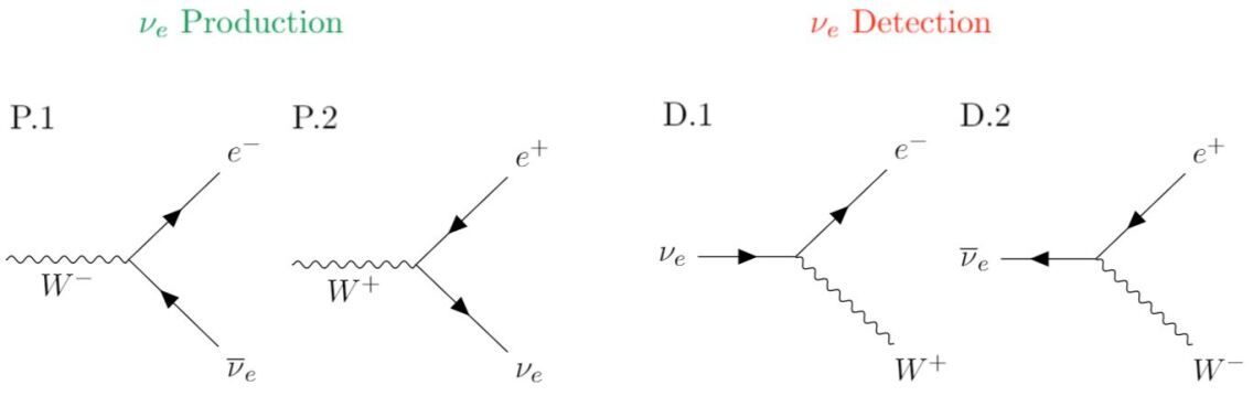
Figure 1: The allowed interactions of electron neutrinos and antineutrinos.

The discovery of anti-neutrinos (seen long before neutrinos) was first made using the process P.1 of Fig. 1 to produce $\bar{\nu}_{e}$ from nuclear reactors, and process D.2 for $\bar{\nu}_{e}$ detection. The schematic outline of the nobel-prize winning 1955 experiment, called “Project Poltergeist” [13], is shown in Fig. 2, top. Electron antineutrinos are produced in $\beta^{-}$ decays within a nuclear reactor. They propagate to a liquid scintillator, where some small fraction undergo “inverse beta decay”, creating a positron and a free neutron. The positron scintillates immediately and the neutron bounces around and eventually captures producing a delayed, detectable signature. This double pulse signature in liquid scintillator is characteristic of low energy antineutrino detection. Seeing such events with rates correlated with reactor activity led to the conclusive discovery of the anti-neutrino.

If the neutrino is equivalent to the anti-neutrino then in principle we might imagine another process, where we first produce a $\bar{\nu}_{e}$ alongside an $e^{-}$ (we look at the electron so we know it was produced as an antineutrino), but we see it interact as if it were a $\nu_{e}$, producing another $e^{-}$ (we look at the electron so we know it interacted as a neutrino). Clearly such a process would violate lepton number conservation, since we had no leptons (L=0) in the beginning and we have two electrons (L=2) the end. This lepton number violation is the hallmark of Majorana neutrinos. Observing this hypothetical process, shown in Fig. 2, bottom, would establish the neutrino as a Majorana fermion using a neutrino beam, and earn us an all expenses paid ticket to Stockholm.

Neutrino discovery channel by Project Poltergeist

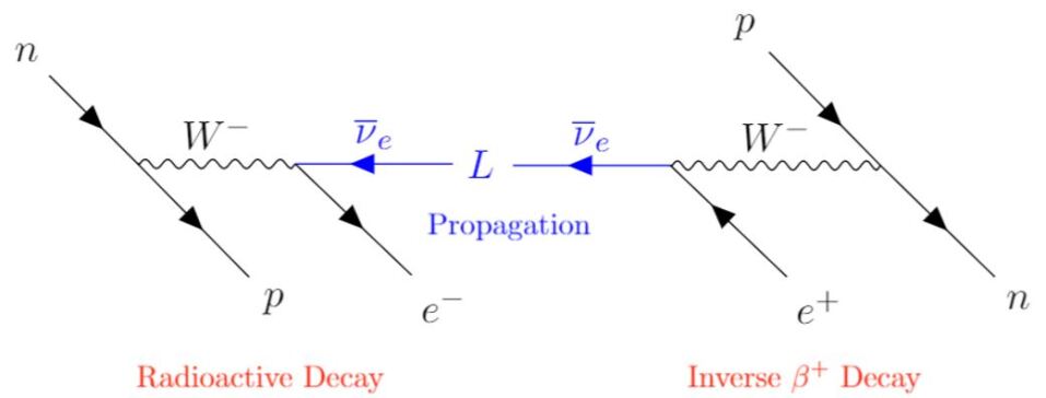
Possible detection channel if neutrinos are their own antiparticles?

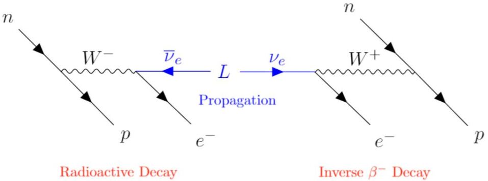
Figure 2: Top: The process by which the neutrino was first detected by Project Poltergeist - electron neutrino production by beta decay followed by electron neutrino detection by inverse $\beta^{+}$ decay. Bottom: A similar process that we might imagine could be allowed if neutrinos are their own antiparticles. .

When we delve a little deeper, we find that this experiment that looks so easy, is in fact, not so. It is thwarted by the competing forces of the chiral structure of weak interactions and angular momentum conservation. Recall that weak interactions have a vector-minus-axial-vector (V-A) structure, which means that the fermion currents in these Feynman amplitudes have a $\gamma^{\mu}\left[1-\gamma^{5}\right]$ sandwiched between two fermion fields. Mathematically the current at the first neutrino interaction vertex looks like:

$$\bar{u}_{e}\frac{1}{2}\gamma^{\mu}\left[1-\gamma^{5}\right]v_{\nu}=\bar{u}_{e}\gamma^{\mu}P_{L}v_{\nu}.$$ (23)

On the other hand, the one at the second neutrino interaction vertex looks like:

$$\bar{v}_{e}\frac{1}{2}\gamma^{\mu}\left[1-\gamma^{5}\right]u_{\nu}=\bar{v}_{e}\gamma^{\mu}P_{L}u_{\nu}.$$ (24)

Recall also that most confusing of factoids from that class you once took on particle physics: $P_{L}$ selects the left chiral parts of particle spinors and the right chiral parts of anti-spinors (Thomson [1] P140). Thus the outgoing neutrino-like thing at the left vertex must be left-chiral, and the incoming antineutrino-like thing at the right vertex must be right chiral, per the utterly screwy preferences of the weak interaction.

The chiralities of the emitted and detected things don’t match, so we would be dead in the water with this experiment if chirality were a conserved quantity. Luckily we have seen that chirality is not conserved for massive fermions, so maybe it’s ok. What might be a problem though, is that the neutrino’s social mobility is severely limited by considerations of helicity.

Recall that in the ultra-relativistic limit, when $m\ll E$, helicity and chirality are equivalent. In this limit, the emerging “antineutrino-like thing” at the left vertex would have to be right-helicity, which means having spin pointing left-to-right in this picture; whereas the entering “neutrino-like thing” at the right vertex would have to be left-helicity, meaning spin pointing right-to-left. This change of spin mid-flight, assuming the neutrino doesn’t interact with anything on the way, is prohibited by angular momentum conservation. And, even if we have Majorana neutrinos we still have angular momentum conservation. So for a massless neutrino this process would surely be prohibited.

Only in the case where the neutrino is somewhat non-relativistic and chirality and helicity are inequivalent can this process occur without violating spin conservation. In this case, the neutrino leaving the left vertex (left chiral) has a small but non-zero right helicity component. Explicitly, for high energy particles the decomposition of chiral states $u_{L,R}$ in terms of helicity $u_{\uparrow,\downarrow}$ states takes the form, for example for u_L:

$$u_{L}=\frac{1}{2}\left(1+\kappa\right)u_{\uparrow}+\frac{1}{2}\left(1-\kappa\right)u_{\downarrow},\quad\quad\kappa\sim\left(1-\frac{m}{E}\right).$$ (25)

Neutrinos are very light, so always very relativistic, and this implies their $\kappa$ is very close to 1. The tiny $u_{\downarrow}$ component, proportional to $m_{\nu}/E_{\nu}$, is what can allow the process we have sketched out to proceed. We can use this information to estimate the rate of this process relative to the “boring” lepton-number-conserving one that was used to discover the antineutrino. Rates of processes are proportional to the squares of their amplitudes, by Fermi’s Golden Rule. Our hypothesized lepton-number-violating ($\Delta L=2$) process will thus be suppressed relative to the Standard Model lepton-number-conserving ($\Delta L=0$) process by a factor $m_{\nu}^{2}/E^{2}$.

We don’t know the neutrino mass, but we do know for sure that it is less than around 1eV [14]. If we consider reactor neutrino experiments [15], the beams have energy of a few MeV. Thus, at most one in every $\sim 2\times 10^{13}$ neutrinos that interact at all, might interact according to our hypothetical lepton-number-violating mode. The rest will interact via the good-old-fashioned, salt-of-the-Earth lepton number conserving mode, even if neutrinos are indeed Majorana fermions.

And here lies the rub: unfortunately, probing processes that are suppressed by factors of more than $10^{12}$ remains far outside the statistical reach of even the most barn-burning reactor neutrino experiments, which collect around 400 interactions per day. Accelerator and atmospheric neutrino experiments can’t help either - their event rates are also far from sufficient, and the energies are even higher, given an even large rate suppression for the L=2 process. Worse still, even if we could detect the $10^{13}$ neutrino interactions needed to have a high probability of observing this new process one time, the prospect of suppressing backgrounds from the standard model process to the part per trillion level sounds basically insane, far beyond any existing experimental capabilities.

Alas, our thought experiment is probably not a viable way to detect Majorana neutrinos. But perhaps it can serve as a guidepost toward a more viable approach.

3.2 The ultimate short baseline experiment

Consider the process shown in (Fig. 3). In this process, a nucleus emits a $W$ boson, turning a neutron into a proton. This creates an electron and an antineutrino; this neutrino propagates a very short distance (on the order of the size of a nucleus), and if Majorana, interacts again with the same nucleus. The ultimate result is production of two electrons, while turning two neutrons into two protons. This process is the exact analog of the hypothetical lepton number violating process we discussed above, but with a baseline smaller than the size of a nucleus. This process is called neutrino-less double beta decay, $0\nu\beta\beta$ for short, and searching for it is the most compelling known way to test for the Majorana nature of the neutrino.

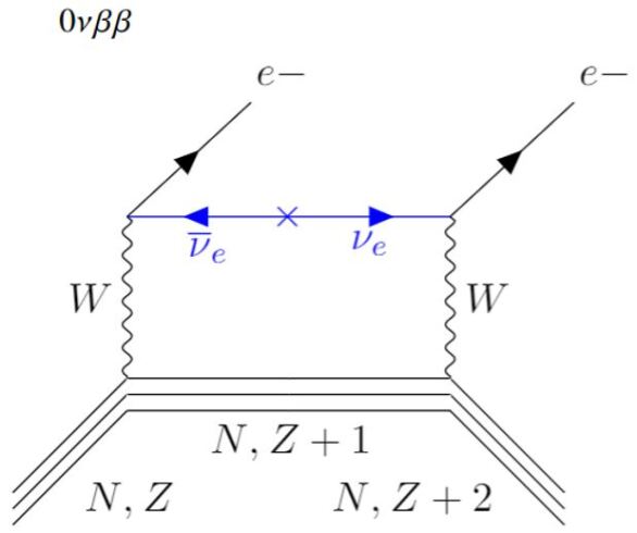
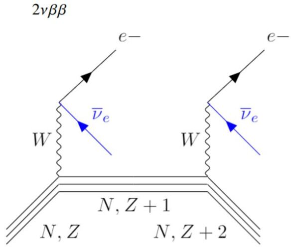
Figure 3: The Feynman diagram for neutrino-less double beta decay (left) and two neutrino double beta decay (right)

It is worth taking a moment to muse on the question, why might this process be any different from the one we discussed before, in terms of plausibility of detection? Are we not again simply overwhelmed with background from a similar $\Delta L$=0 process with the “right-sign” leptons, and $e^{+}e^{-}$ in the final state, as before? The answer can be found by considering what happens to the nucleus in this situation. We would, in that case, need to turn a proton to a neutron and back again. Assuming we start in the ground state of the nucleus as in ordinary matter, our only option would be to change one nucleus into a similar looking one, but with one more proton one and one less neutron, and then flip this one back to exactly where we started. No other final state is energetically accessible from the ground state. In this process there would be no free energy to put into the electrons, apart from a tiny quantity of order a few eV absorbed by the nuclear recoil. For the process to go, we would need at least enough energy difference available between the initial and final nuclear states to make two electron masses, however - with zero available energy, the two new electrons simply cannot be created.

On the other hand, the $\Delta L$=2 process where two neutrons change into two protons actually transforms the nucleus into a different one. If we pick a nucleus where a heavier isotope would turn into a lighter one when two neutrons turned into two protons, we have a setup that seems almost custom-made for driving forward the lepton-number-violating $\Delta L=2$ process while suppressing its lepton-number-conserving $\Delta L=0$ counterpart. In such a system, the energy released can be converted into electron mass energy and kinetic energy in the two-electron final state.

3.3 The pairing force as the engine of double beta decay

The effect that makes searching for this weird nuclear decay a viable possibility rather than science fiction is the nuclear pairing force. Nucleons in nuclei have spin, and so they have magnetic moments. Just like electrons in atomic orbitals, it is usually energetically favorable for them to pair up with spins opposing each-other in equivalent spatial orbitals. This maximizes wave-function overlap and the stabilizing effect of the attractive spin-opposite spin interaction. The result is that nuclei with even numbers of protons, or even numbers of neutrons, are nearly always slightly more tightly bound than similar nuclei with odd numbers of both. In then yet more special even-even nuclei where both proton and neutron numbers are even, all of the nucleons can pair up in this harmonious, stabilizing way.

   

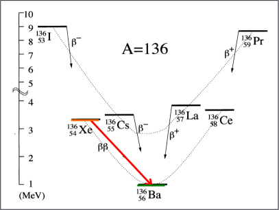
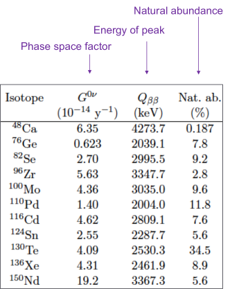
Figure 4: Left: Masses of isotopes in the N=136 isobar. Right: table of phase space factors, Q-values, and natural abundances of double beta decaying nuclei.

Beta decays, of either the single or double variety, never change the total number of nucleons in a nucleus (this would violate baryon number, which is never violated perturbatively in the standard model). So beta decays always move us within an “isobar”, that is, the collection of nuclei with the same total number of nucleons N but different numbers of protons Z. When we plot the mass of the nucleus vs the number of protons within an isobar, we immediately see the effect of the nuclear pairing force. Figure 4, left shows an example. Even-even nuclei ¹³⁶Xe and ¹³⁶Ba are stabilized by pairing. Odd-odd nuclei ¹³⁶I and ¹³⁶Cs are less tightly bound. The result is that ¹³⁶Xe is energetically forbidden from undergoing single beta decay to ¹³⁶Cs, but is energetically allowed to double beta decay to ¹³⁶Ba. This makes ¹³⁶Xe an example of an outstanding nucleus we might be able to use as a laboratory to search for $0\nu\beta\beta$. There are a handful of such nuclei where the nuclear pairing force makes the energetics work just-so, some examples given in Fig. 4, right. So maybe the Nobel-worthy experiment we dreamed up in the last section can work after all, if we make our neutrino baseline smaller than the size of the nucleus.

Not so fast - just like the earlier thought experiment, of course, the rate of $0\nu\beta\beta$ is still suppressed by a factor of $m^{2}/E^{2}$. This is because the neutrino still has to interact with the “wrong” helicity at the second vertex. Naturally if $m_{\nu}=0$, the neutrino would have no “wrong helicity” component and so the rate of $0\nu\beta\beta$ would be zero. The rate would also be zero if the neutrino mass is finite but the neutrino is not Majorana. Only if the neutrino is both massive and Majorana, can $0\nu\beta\beta$ proceed with a non-zero rate, and the suppression by $m^{2}/E^{2}$ means that the rate of this decay is going to be slow as heck. Since we don’t yet know the neutrino mass we don’t know what decay rate is expected, but existing constraints imply a decay half-life to the neutrinoless mode of at least $\geq 10^{26}$ years in most practical isotopes.

3.4 Neutrinoless and two neutrino double beta decay

Although we don’t suffer from the “non-helicity-flipping” background of our earlier thought experiment, there is still a decay process of even-even isotopes that does represent a challenging background to $0\nu\beta\beta$ . This is two neutrino double beta decay, an event where two ordinary beta decays happen at once, with two electrons and two neutrinos in the final state. The $2\nu\beta\beta$ mode goes at least $10^{6}$ times faster (in xenon) than the predicted rate of the $0\nu\beta\beta$ mode. Diagrams of this processes are shown in Fig. 3, right.

What are we going to do about this background? Well, the final state of this two-neutrino process is rather different from the process we are interested in. It has two electrons and two neutrinos, whereas the $0\nu\beta\beta$ has only two electrons. The question is whether we can we tell the difference reliably enough to reject backgrounds with this different final state. Answering this question positively is the first criterion for a sensitive $0\nu\beta\beta$ experiment.

Naively we might imagine telling the difference between the two modes by detecting the neutrinos and vetoing the events that have them. However, given the interaction cross sections of neutrinos at this energy, to reliably tag an emerging neutrino would require a block of detector material of around a light year in length - not a very viable prospect. It seems we are restricted to only measuring the charged decay products: the electrons and possibly the daughter nucleus.

But there is still a difference between the final states of $0\nu\beta\beta$ and $2\nu\beta\beta$, even if we can only measure the electrons. In the case of the two neutrino mode, the available energy is shared between two detectable electrons and two unobservable neutrinos. In the case of the neutrino-less mode, all the energy is directed into the electrons. Since the amount of energy available is fixed - it is the mass difference between the parent and daughter nuclei - the neutrino-less mode should produce a mono-energetic spike, whereas the two-neutrino mode produces a broad spectrum.

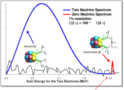
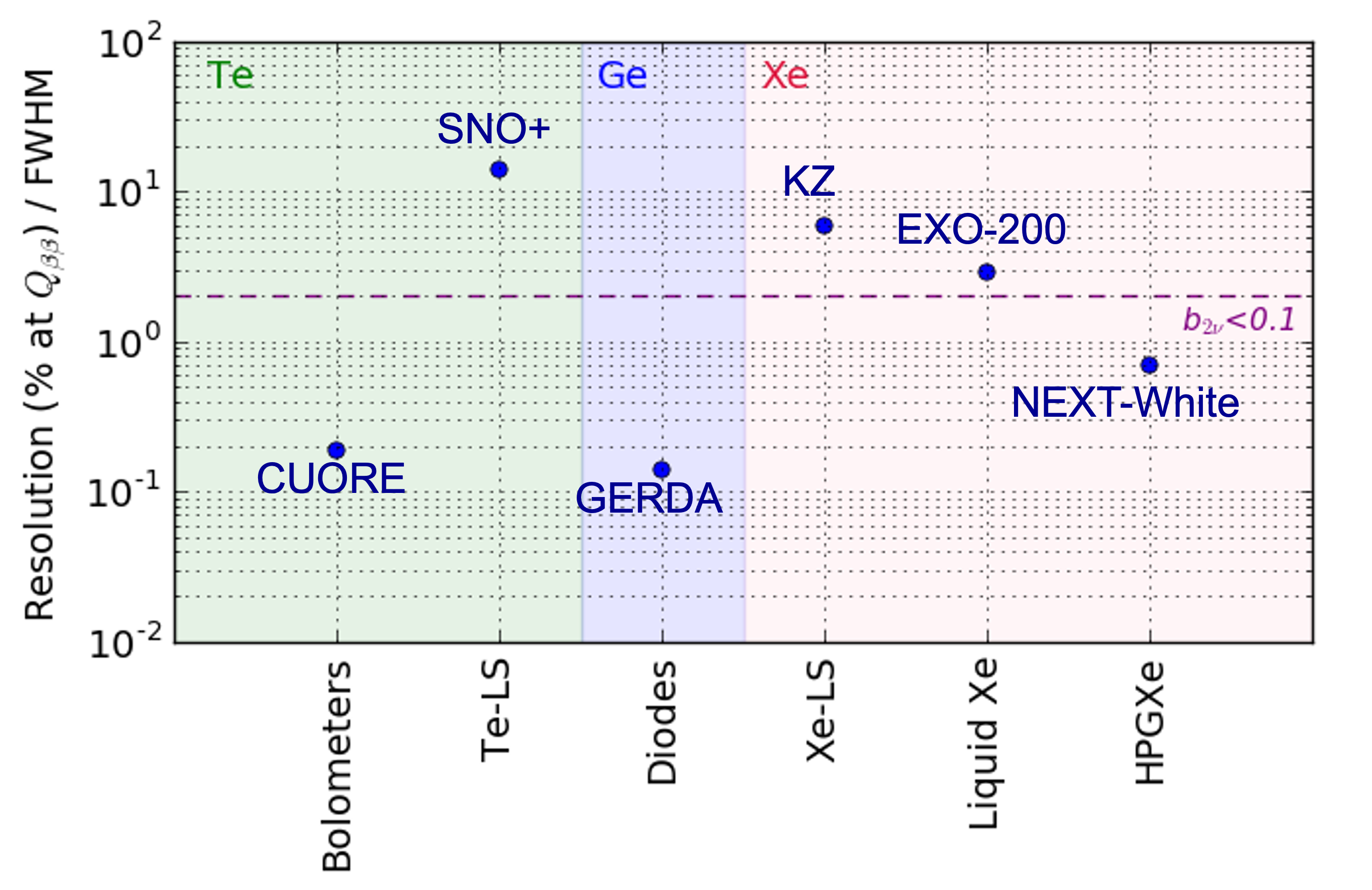
Figure 5: Left: Spectrum of energy emitted into electrons in the two-neutrino and neutrino-less modes of double beta decay. . Right: demonstrated energy resolutions in various detector technologies, tellurium bolometers, tellurium in liquid scintillator, germanium diodes, xenon in liquid scintillator, high pressre xenon gas.

While the energy is in general shared between final state particles, its sharing is inherently random. It is possible to have almost all the energy in the electrons and almost none in the neutrinos. Thus there is a tail to the $2\nu\beta\beta$ spectrum that runs almost (up to two neutrino masses) all the way up to the hypothetical $0\nu\beta\beta$ peak. In order not to incorporate background from this tail, exquisite energy resolution in the electron energy measurement is required.

In order to to reduce the background from $2\nu\beta\beta$ in the $0\nu\beta\beta$ region of interest to a suitable level, generally agreed by the community to be around 0.1 counts per ton per year, next-generation $0\nu\beta\beta$ experiments require energy resolution of at most most 2% FWHM. More precise resolutions protect from the effects of inevitable non-Gaussian tails in energy distributions. The energy resolutions demonstrated in various technologies to date are shown in Fig. 5, right. Several of them comfortably meet this goal; others still suffer from $2\nu\beta\beta$ backgrounds in their energy regions of interest. Progress toward ever longer lifetime sensitivities will require this background to be ever more efficiently mitigated via precise energy resolution, if it is not to become an irreducible barrier to sensitivity.

4 The rate of $0\nu\beta\beta$

Calculating the rate of either neutrinoless or two-neutrino double beta decay is a tricky business, because it involves understanding the properties of the nucleus that is undergoing decay. Here we present a valiant attempt that illustrates a lot of the key physics, but necessarily involves skipping steps and making simplifications that are not made in modern theoretical calculations. I regret nothing. Let us start with the Hamiltonian, following Refs. [6, 17]:

$$H=\left(\sqrt{2}G_{F}\left|V_{ud}\right|\right)^{2}\left[\bar{e}_{L}\gamma_{\mu}(1-\gamma_{5})\nu_{L}\right]\left[-\bar{\nu}_{L}^{c}\gamma_{\mu}(1-\gamma_{5})e_{L}^{c}\right]\left[\bar{p}\gamma^{\mu}(1-g_{A}\gamma_{5})n\right]\left[\bar{p}\gamma^{\mu}(1-g_{A}\gamma_{5})n\right]$$ (26)

Many elements of this object are familiar; we have the Fermi constant twice - expected for a second order weak process; the CKM matrix element $|V_{ud}|$, since the $W$ bosons here couple u quarks to d quarks; Two terms for leptonic vertices, though one of them is a bit weird looking compared to what we might expect in a more garden-variety process due to those conjugate operations - we will be contracting this with the other term to form a propagator soon; and then two hadronic currents that turn protons into neutrons. We also see the weak vertex terms: $\gamma^{\mu}(1-\gamma_{5})$ as expected at the leptonic vertices, but $\gamma^{\mu}(1-g_{A}\gamma_{5})$ at the hadronic ones. It is worth taking a brief digression to explain this, since the value of $g_{A}$ is an ongoing topic of discussion you might hear about, in connection with theoretical predictions of the rate of double beta decay theory.

4.1 The role of vector / axial vector currents and $g_{A}$

Why in the vertex for the nucleon did the vector part have a coupling strength of 1, as in the leptonic sector, but the axial part have a coupling strength of $g_{A}$? Before asking why the axial coefficient is modified but the vector one is not, we can ask a more pressing question - why would any of these coefficients not be 1? The weak charged current interaction couples like $\gamma^{\mu}(1-\gamma_{5})$, right? What is this $g_{A}$?

The answer is that nuclear effects, such as meson exchange currents in the nuclear medium, affect the strength of the couplings that drive beta decay within the nucleus. This can make life miserable for everyone, even talented nuclear theorists. Some examples of these processes are shown in Fig. 6. The consequence is that the neutrino never really interacts with just one nucleon in a vacuum, it interacts with a nucleon that is mid-interaction with all the other nucleons all the time, and so the charges that couple to the weak interaction are not just 1 as they would be for single, fundamental particle interactions.

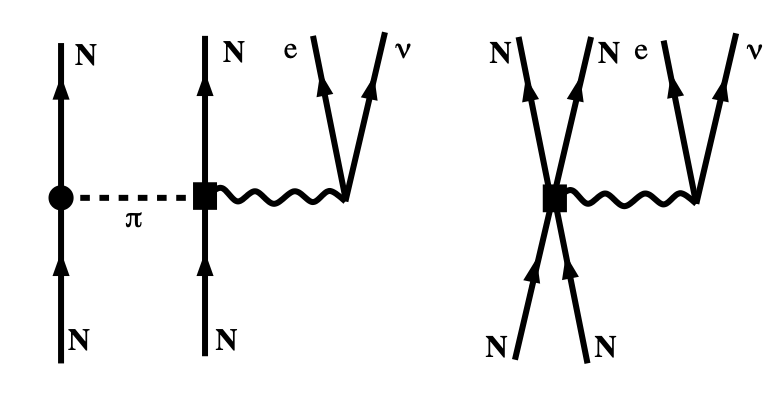
Figure 6: Meson exchange currents that “renormalize” $g_{A}$ in beta decay.

The next question is why the axial charge seems to be modified in the above expression, but not the vector charge. The reason a mysterious thing called the Conservation of Vector Current (CVC) hypothesis. It is an idea greatly pre-dates the standard model itself, but seems to be largely robust even with all the new effects the full standard model of weak interactions piles on top of the old assumptions about nucleons.

Consider the proton and neutron as a doublet in isospin, such that:

$$\Psi=\left(\begin{array}[]{c}p\\ n\end{array}\right).$$ (27)

Under this construction, these two particles are simply manifestations of a simpler, more general particle, the nucleon, differing only in that they have a different position in the isospin doublet. People used to think about them that way, and it turns out that to a good degree of approximation, they behave so, especially in scenarios where the strong interaction is the dominant force. The 3-component of isospin $T_{3}$ of the proton and neutron are determined by applying $\tau_{3}$, which is just the Pauli matrix $\sigma_{3}$ with a fancy name, to make sure we remember it acts in isospin space and not in spin space:

$$\tau_{3}p=\tau_{3}\left(\begin{array}[]{c}1\\ 0\end{array}\right)=+\left(\begin{array}[]{c}1\\ 0\end{array}\right),\quad T_{3}(p)=+1.$$ (32)

$$\tau_{3}n=\tau_{3}\left(\begin{array}[]{c}0\\ 1\end{array}\right)=-\left(\begin{array}[]{c}0\\ 1\end{array}\right),\quad T_{3}(n)=-1.$$ (37)

The electromagnetic current that couples photons to nucleons only notices the proton, since the neutron is neutral. Thus we can write the coupling to the photon field $A_{\mu}$ as:

$$\left[\bar{p}\gamma^{\mu}p\right]A_{\mu}=\left[1\times\bar{p}\gamma^{\mu}p+0\times\bar{n}\gamma^{\mu}n\right]A_{\mu}=J_{EM}^{\mu}A_{\mu}.$$ (38)

In terms of isospin projectors, the electromagnetic current is given by:

$$J_{EM}^{\mu}=\bar{\Psi}\left(1+\tau_{3}\right)\gamma^{\mu}\Psi,$$ (39)

$$=\bar{\Psi}\gamma^{\mu}\Psi+\bar{\Psi}\gamma^{\mu}\tau_{3}\Psi,$$ (40)

$$=g_{I}J_{iso-scalar}+g_{V}J_{3}.$$ (41)

Where in the second equality the current is broken up into an isoscalar part, and a part that depends on the third isospin matrix $\tau_{3}$, and we injected a $g_{I}=1$ and a $g_{V}=1$. The second term can be thought of as the third element in a 3-vector in isospin space, involving $\left(\tau_{1},\tau_{2},\tau_{3}\right)$.

Were isospin really an exact symmetry, that is, protons and neutrons are essentially the same except for their difference in isospin, then isospin would itself be a conserved quantity.

$$\partial_{\mu}J^{\mu}=\partial_{\mu}\bar{\Psi}\vec{\tau}\gamma^{\mu}\Psi=0.$$ (42)

That this is nearly true is in fact why such a weird thing as isospin was ever useful to anyone; all the nucleons in all the nuclei are sufficiently similar to one another from the point of view of the strong force that this conservation law appears true in a great number of scenarios, especially those whose dynamics are dictated dominantly by strong interactions; in others it is broken by a little bit. But renormalization of the nuclear charges, what we are talking about right now, is governed by strong interactions.

Eq. 42 is in fact not one conservation law but three, one for each element in $\vec{\tau}$. Thats one way to look at the situation, anyway. Another is to say, this is one conservation law but of a vector quantity $\vec{\tau}$. To the extent that isospin is a good symmetry, rotating the direction of all the $\vec{\tau}$’s of all the particles by some fixed angle would lead to an equally viable universe that would obey the same laws as our own, albeit starting from a different initial condition. It is hard to imagine such a universe; but were the strong interaction calling all the shots this weird thought experiment would work out just fine.

What does all this have to do with renormalization of weak processes? Well, intriguingly, the currents that couple to the W boson in double beta decay involve isospin raising and lowering operators constructed in terms of other elements of that same isospin vector, just different components:

$$J_{Weak}^{\mu}=g_{V}\bar{\Psi}\left(\tau_{1}\pm i\tau_{2}\right)\gamma^{\mu}\Psi-g_{A}\bar{\Psi}\left(\tau_{1}\pm i\tau_{2}\right)\gamma^{5}\gamma^{\mu}\Psi$$ (43)

$$=g_{V}J_{Weak,V}^{\mu}-g_{A}J_{Weak,A}^{\mu}$$ (44)

Which has been split into vector and axial vector parts, $J_{Weak,V}^{\mu}=J_{1,V}\pm iJ_{2,V}$ and $J_{Weak,A}^{\mu}=J_{1,A}\pm iJ_{2,A}$ Even though they couple to different gauge bosons than the electromagnetic current, and generate apparently different phenomena, the vector parts they invoke are just like the electromagnetic currents, but with different elements of the $\vec{\tau}$ vector. No matter what weird QCD stuff happens, higher order nuclear effects cannot modify the charge of nucleon, since whatever stuff those effects might violate they surely conserve charge. Thus the electromagnetic current, Eq. 41 is unmodified by nuclear effects. If isospin symmetry is really a symmetry, then, the $g_{V}$ in Eq. 41 is also unmodified by higher order nuclear effects - it is driven by the same kind of currents, just with a different choice of direction for the isospin vector $\vec{\tau}$. This is the consequence of CVC hypothesis in $0\nu\beta\beta$ - to the extent that isopsin is a good symmetry, $g_{V}=1$ even with nuclear effects.

On the other hand, all bets are off concerning $g_{A}$. This quantity is not related to anything to do with electromagnetism and is not protected by the principle of CVC. Generally one expects it to be modified by potentially large amounts, due to higher order nuclear effects. Since $g_{A}$ will feature to the fourth power in the rate of $0\nu\beta\beta$, even small changes to it matter a lot.

The theoretical treatments are evolving. For the present moment, $g_{A}$ is a significant source of uncertainty in the nuclear currents involved in double beta decay. Measurements from neutron decay (a decay which also involves both vector and axial vector parts) presently give the most precise value, $g_{A}\sim 1.27$. However, it is debatable whether this can be taken as an accurate value for the complex nuclei involved in neutrinoless double beta decay experiments. Two-neutrino double beta decay rates suggest that $g_{A}$ could be significantly modified relative to neutron decay. The most modern matrix element methods claim a self-consistent calculation which incorporates the effects of $g_{A}$ fully. It seems reasonable to be hopeful for a conclusive resolution of the question renormalization of $g_{A}$ question in the relatively near future.

4.2 The leptonic and hadronic tensors in single light neutrino exchange

The Hamiltonian Eq. 26 can be taken as being a reasonable one for both two-neutrino and neutrinoless decays. In the case of neutrinoless double beta decay, the neutrino that is emitted at one vertex is absorbed at the other one. In quantum field theory this corresponds to replacing the two $\nu$ fields in the above expression with a fermionic propagator, and it turns out that the propagator here is the same one we would expect for Dirac fermions [17]:

$$\frac{\not{k}+m}{k^{2}-m^{2}}.$$ (45)

The matrix element for the process then takes the form:

$${\cal M}=-2G_{F}^{2}\left|V_{ud}\right|^{2}\sum_{n}\int\frac{d^{4}k}{\left(2\pi\right)^{4}}\bar{u}(p_{1})\frac{1-\gamma_{5}}{2}\gamma_{\mu}\frac{\not{k}_{\nu}+m}{k_{\nu}^{2}-m^{2}}\gamma_{\nu}\frac{1-\gamma_{5}}{2}v(p_{2})e^{i\vec{k}_{\nu}.r}\times$$ (46)

$$\langle N_{i}|J^{\mu}|n\rangle\langle n|J^{\nu}|N_{f}\rangle 2\pi\delta(k_{\nu}-E_{1i}+E_{1n}+\epsilon_{1}).$$ (47)

Where $|n\rangle$ is the intermediate state of the nucleus. This can be written in terms of a hadronic and a leptonic part:

$$=-2G_{F}^{2}\left|V_{ud}\right|^{2}\sum_{n}L_{\mu\nu}^{n}H_{n}^{\mu\nu}.$$ (48)

The leptonic part has a form that looks like it might be manageable:

$$L^{\mu\nu}=\int\frac{d^{4}k}{\left(2\pi\right)^{4}}\bar{u}(p_{1})\frac{1-\gamma_{5}}{2}\gamma_{\mu}\frac{\not{k}_{\nu}+m_{\nu}}{k_{\nu}^{2}-m_{\nu}^{2}}\gamma_{\nu}\frac{1-\gamma_{5}}{2}v(p_{2})e^{i\vec{k}_{\nu}.r}.$$ (49)

Considering for a moment the two added terms in the propagator, we see that the two chiral projectors force us to keep only the $m_{\nu}$ term, since:

$$\frac{1-\gamma_{5}}{2}\gamma_{\mu}\not{k}_{\nu}\gamma_{\nu}\frac{1-\gamma_{5}}{2}=\gamma_{\mu}\frac{1+\gamma_{5}}{2}\not{k}_{\nu}\gamma_{\nu}\frac{1-\gamma_{5}}{2}=\gamma_{\mu}\not{k}_{\nu}\frac{1-\gamma_{5}}{2}\gamma_{\nu}\frac{1-\gamma_{5}}{2}$$ (50)

$$=\gamma_{\mu}\not{k}_{\nu}\gamma_{\nu}\frac{1+\gamma_{5}}{2}\frac{1-\gamma_{5}}{2}=0.$$ (51)

So, we find:

$$L^{\mu\nu}=m_{\nu}\int\frac{d^{4}k}{\left(2\pi\right)^{4}}\frac{1}{k_{\nu}^{2}-m_{\nu}^{2}}\bar{u}(p_{1})\gamma_{\mu}\gamma_{\nu}\frac{1-\gamma_{5}}{2}v(p_{2})e^{i\vec{k}_{\nu}.r}.$$ (52)

Note that if $m_{\nu}=0$ then $L^{\mu\nu}=0$ and the process cannot go, as expected. Next we can use momentum balance in the denominator of the propagator to set:

$$k_{\nu}^{2}-m_{\nu}^{2}=(p_{1i}-p_{n}-p_{1})^{2}-m_{\nu}^{2}.$$ (53)

In this expression, $p_{1i}$ is the initial momentum of nucleon 1; $p_{n}$ is the momentum of the intermediate state; and $p_{1}$ is the momentum of the outgoing electron. Continuing to re-organize:

$$=(E_{1i}-E_{n}-E_{1})^{2}-(\vec{p}_{1i}-\vec{p}_{n}-\vec{p}_{1})^{2}-m_{\nu}^{2}$$ (54)

$$=(E_{1i}-E_{n}-E_{1})^{2}-\left(\vec{k}_{\nu}^{2}+m_{\nu}^{2}\right)$$ (55)

$$=(E_{1i}-E_{n}-E_{1})^{2}-\epsilon_{\nu}^{2}.$$ (56)

Where here $\epsilon_{\nu}$ is the energy of the virtual neutrino. Continuing to manipulate the leptonic current, we can use the identity:

$$\gamma^{\mu}\gamma^{\nu}=\eta^{\mu\nu}+\frac{1}{2}\sigma^{\mu\nu},\quad\quad(\sigma^{\mu\nu}=\frac{1}{2}[\gamma^{\mu},\gamma^{\nu}]).$$ (57)

to simplify the leptonic tensor:

$$\\ L_{n}^{\mu\nu}=m_{\nu}\int\frac{d^{4}k}{\left(2\pi\right)^{4}}\frac{1}{k_{\nu}^{2}-m_{\nu}^{2}}\bar{u}(p_{1})\left(\eta^{\mu\nu}+\sigma^{\mu\nu}\right)\frac{1-\gamma_{5}}{2}v(p_{2})e^{i\vec{k}_{\nu}.r}.$$ (58)

For super-allowed transitions, $0^{+}\rightarrow 0^{+}$ there is no “magnetic” contribution and so we can drop the term proportional to $\sigma^{\mu\nu}$. This leaves us with:

$$L_{n}^{\mu\nu}=m_{\nu}\eta^{\mu\nu}\int\frac{d^{4}k}{\left(2\pi\right)^{4}}\frac{1}{(E_{1i}-E_{n}-E_{1})^{2}-\epsilon_{\nu}^{2}}\bar{u}(p_{1})\frac{1-\gamma_{5}}{2}v(p_{2})e^{i\vec{k}_{\nu}.r}.$$ (59)

To do the sum over intermediate states $|n\rangle$ it is typical to invoke an approximation called the “closure” approximation. This is believed to work well for neutrinoless double beta decay rates but not so well for two-neutrino double beta decays. The basis of the approximation is that if it is reasonable to consider all the intermediate states have approximately the “mean” intermediate state energy $E_{n}\sim\langle E\rangle$ then the weighted sum that appears in the decay rate simplifies considerably:

$$\sum_{n}\frac{\langle N_{f}|J_{1}|n\rangle\langle n|J_{2}|N_{i}\rangle}{(E_{i}-E_{n}-E_{\eta}-E_{\nu})}\rightarrow\frac{\langle N_{f}|J_{1}\left(\sum_{n}|n\rangle\langle n|\right)J_{2}|N_{i}\rangle}{(E_{i}-\langle E_{n}\rangle-E_{\eta}-E_{\nu})}.$$ (60)

Because the sum is over a complete set of states, $\sum_{n}|n\rangle\langle n|=1$ and so:

$$\sum_{n}\frac{\langle N_{f}|J_{1}|n\rangle\langle n|J_{2}|N_{i}\rangle}{(E_{i}-E_{n}-E_{\eta}-E_{\nu})}\rightarrow\frac{\langle N_{f}|J_{1}J_{2}|N_{i}\rangle}{(E_{i}-\langle E_{n}\rangle-E_{\eta}-E_{\nu})}.$$ (61)

Making this approximation we can now factorize the matrix element into hadronic and leptonic tensors:

$$M=-2G_{F}^{2}\left|V_{ud}\right|^{2}\sum_{n}L_{\mu\nu}^{n}H_{n}^{\mu\nu}\rightarrow-2G_{F}^{2}\left|V_{ud}\right|^{2}L_{\mu\nu}H^{\mu\nu}$$ (62)

And so the spin-summed matrix element squared needed to calculate a decay rate factorizes like:

$$\langle|M|^{2}\rangle=4G_{F}^{4}\left|V_{ud}\right|^{4}\left(\sum_{spins}L_{\sigma\rho}L_{\mu\nu}\right)\left(H^{\sigma\rho}H^{\mu\nu}\right).$$ (63)

Note that each $H$ here contains two powers of $g_{A}$, so the total number of powers of $g_{A}$ in the expression is four. Following a few familiar contractions and lines of rearrangement, we can get the spin summed product of $L$’s, as:

$$\sum_{spins}L_{\sigma\rho}L_{\mu\nu}=m_{\nu}^{2}g_{\mu\nu}g_{\sigma\rho}Tr\left[\left(\not{p}_{1}+m_{e}\right)\left(\frac{1+\gamma^{5}}{2}\right)\left(\not{p}_{2}-m_{e}\right)\left(\frac{1-\gamma^{5}}{2}\right)\right].$$ (64)

In this trace, only the elements with both $p$’s survive:

$$=m_{\nu}^{2}g_{\mu\nu}g_{\rho\sigma}(4g_{\alpha\beta}p_{1\alpha}p_{2\beta})$$ (65)

$$=4m_{\nu}^{2}g_{\mu\nu}g_{\rho\sigma}p_{1}.p_{2}.$$ (66)

And this can be used to evaluate the matrix element:

$$\langle|{\cal M}|^{2}\rangle=4G_{F}^{2}\left|V_{ud}\right|^{4}H_{\mu}^{\mu}H_{\rho}^{\rho}m_{\nu}^{2}2p_{1}.p_{2}\left[\frac{1}{4\pi}F(r)\right]^{2}.$$ (67)

$$F(r)=\frac{1}{4\pi^{2}}\sum_{\eta=1}^{2}\int d^{3}k_{\nu}\frac{e^{ik_{\nu}r}}{(-\epsilon_{\nu})(E_{i}-\langle E_{n}\rangle-E_{\eta}-E_{\nu})}.$$ (68)

This is the expression for the matrix element if we imagine there is only one kind of neutrino participating, with mass $m_{\nu}$.

4.3 Multiple massive neutrinos in the three flavor paradigm

In fact in the process of neutrinoless double beta decay, there are contributions to the decay amplitude from multiple mass eigenstates. Neglecting neutrino masses within the propagators since they are much below the energy scale of the process, but keeping the ones in the numerators, we find an amplitude contribution from each to the matrix element.

For each neutrino, there is an amplitude contribution that will involve two factors of the leptonic mixing matrix (a.k.a the PMNS matrix), and the neutrino mass (collecting into X everything that is not $m_{\nu i}$ of line 67):

$$M_{i}=X\left(U_{ei}\right)^{2}m_{\nu i}.$$ (69)

And so the total matrix element will be the sum of these contributions, which ultimately gets squared in Fermi’s Golden Rule for the decay rate:

$$\left|{\cal M}\right|^{2}=\left|X\sum_{i}(U_{ei})^{2}m_{\nu i}\right|^{2}=\left|X\right|^{2}m_{\beta\beta}^{2}$$ (70)

$$=4G_{F}^{2}\left|V_{ud}\right|^{4}H_{\mu}^{\mu}H_{\rho}^{\rho}2p_{1}.p_{2}\left[\frac{1}{4\pi}F(r)\right]^{2}m_{\beta\beta}^{2}.$$ (71)

Above we have introduced the important effective parameter $m_{\beta\beta}$:

$$m_{\beta\beta}=\sum_{i}(U_{ei})^{2}m_{\nu i}.$$ (72)

Accounting for the matrix element and the final state phase space, the full decay rate takes the form:

$$\frac{d\Gamma}{d\cos\theta\,dE_{1}}=\left\{\frac{G_{F}^{4}\left|V_{ud}\right|^{4}}{16\pi^{5}}E_{1}E_{2}|\vec{p}_{1}||\vec{p}_{2}|\left(1-\frac{\vec{p_{1}}.\vec{p_{2}}}{E_{1}E_{2}}\right)\right\}\times$$ (73)

$$\left\{H_{\mu}^{\mu}H_{\rho}^{\rho}\left[\frac{1}{4\pi}F(r)\right]^{2}\right\}\left\{m_{\beta\beta}^{2}\right\}.$$ (74)

The curly bracketed pieces are called respectively the “Phase Space Factor” (G), the “Nuclear Matrix Element” ($\left\|M\right\|$), and the “Effective Majorana Mass” ($m_{\beta\beta}^{2}$). This is often written in compact form:

$$\Gamma=G\left\|M\right\|{}^{2}m_{\beta\beta}^{2}.$$ (75)

and for what follows we will absorb the couplings and CKM elements into $G$:

$$G=G_{F}^{4}\left|V_{ud}\right|^{4}\tilde{G}.$$ (76)

4.4 The phase space factor

In the simplest version of the calculation of $\tilde{G}$, the kinematic part of $G$, we find:

$$\tilde{G}=\int\frac{1}{16\pi^{5}}dE_{1}d\cos\theta\,E_{1}E_{2}|\vec{p}_{1}||\vec{p}_{2}|\left(1-\frac{\vec{p_{1}}.\vec{p_{2}}}{E_{1}E_{2}}\right).$$ (77)

This is an integral we can evaluate. First, we explicitly include the opening angle:

$$=\int\frac{1}{16\pi^{5}}dE_{1}d\cos\theta\,E_{1}E_{2}|\vec{p}_{1}||\vec{p}_{2}|\left(1-\frac{p_{1}p_{2}}{E_{1}E_{2}}\cos\theta\right).$$ (78)

And note that the integral $\int_{-1}^{1}d\cos\theta\,\cos\theta=0$, so only the left term survives the angular integration:

$$=\frac{1}{8\pi^{5}}\int_{m_{e}}^{m_{e}+T_{0}}dE_{1}E_{1}E_{2}|\vec{p}_{1}||\vec{p}_{2}|,$$ (79)

Now using $E_{2}=T_{0}+2m_{e}-E_{1}$, $p_{1}=\sqrt{E_{1}^{2}+m_{e}^{2}}$ and $p_{2}=\sqrt{E_{2}^{2}+m_{e}^{2}}$ we find:

$$=\frac{1}{8\pi^{5}}\int_{m_{e}}^{m_{e}+T_{0}}dE_{1}E_{1}\left(T_{0}+2m_{e}-E_{1}\right)\sqrt{E_{1}-m_{e}^{2}}\sqrt{\left(T_{0}+2m_{e}-E_{1}\right)^{2}-m_{e}^{2}},$$ (80)

This integral can be done either with blood, sweat and tears, or with Mathematica, with the result that:

$$=\frac{m_{e}^{5}}{8\pi^{5}}\left(\frac{t_{0}^{5}}{30}+\frac{t_{0}^{4}}{3}+\frac{4t_{0}^{3}}{3}+2t_{0}^{2}+t_{0}\right)\quad\quad t_{0}=\frac{T_{0}}{m_{e}},$$ (81)

Where $T_{0}$ is the total available kinetic energy, labelled in table 4 as Q_ββ. Because $T_{0}>m_{e}$, the decay rate scales with the fifth power of the available energy, to leading order, all other things being equal. This is one reason to favor decay isotopes with higher Q-values for experimental study. A second and more pragmatic reason for favoring higher Q_ββ is that the higher the Q-value, the more likely the $0\nu\beta\beta$ is to be above the lines from dominant radiogenic backgrounds.

Eq. 81 is not quite the end of the story for phase space factors since in the full calculation we must also include the Fermi function $F(E,Z)$ to account for the Coulomb attraction of the electron leaving the nucleus [18]. This correction accounts for the fact that the wave function of an electron leaving as a plane wave is distorted by Coulomb attraction at the origin. The corrected expression for $\tilde{G}$ is:

$$\tilde{G}=\int\frac{1}{16\pi^{5}}F(E_{1},Z)F(E_{2},Z)dE_{1}d\cos\theta\,E_{1}E_{2}p_{1}p_{2}\left(1-\frac{\vec{p_{1}}.\vec{p_{2}}}{E_{1}E_{2}}\right)$$ (82)

These coulomb effects must include relativistic corrections and shielding from the atomic electrons, which makes the integral rather more complex. It can be evaluated using numerical methods [19, 20].

4.5 The nuclear matrix element

Calculation of the nuclear matrix elements is far more difficult. Many different techniques exist, requiring vast computation and with tracts of supporting literature. The present status of the field is that the various methods agree on their predictions to within a factor of 2-3. This is improving as more advanced ab-initio methods reach maturity, and the computing power to evaluate them becomes more freely available. Recent reviews of the subject give an excellent coverage of the various methods in common use [9, 21]. The nuclear matrix elements are generally considered the largest of the theoretical uncertainties in predictions of double beta decay rates.

It is notable also that the effects of $g_{A}$ are buried inside these objects, to varying degrees, depending on the computational method chosen. While the uncertainty on $g_{A}$ is sometimes considered as factorized into a separate question from the uncertainty on calculation of the matrix element itself, the two cannot be straightforwardly decoupled. There is evidence from two-neutrino double beta decays that $g_{A}$ as measured in two neutrino decays may be different by a large factor, relative to neutron decay, and this introduces a comparable degree of uncertainty into the predicted rate of $0\nu\beta\beta$ to other aspects of the matrix element calculation. This situation is evolving, and for a relatively modern discussion see Ref [22].

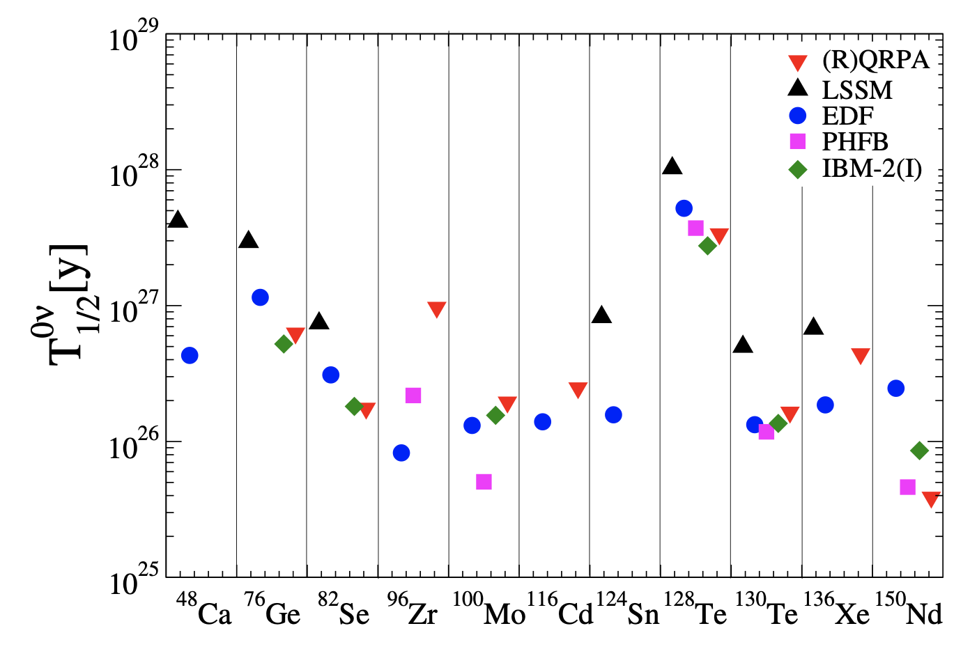
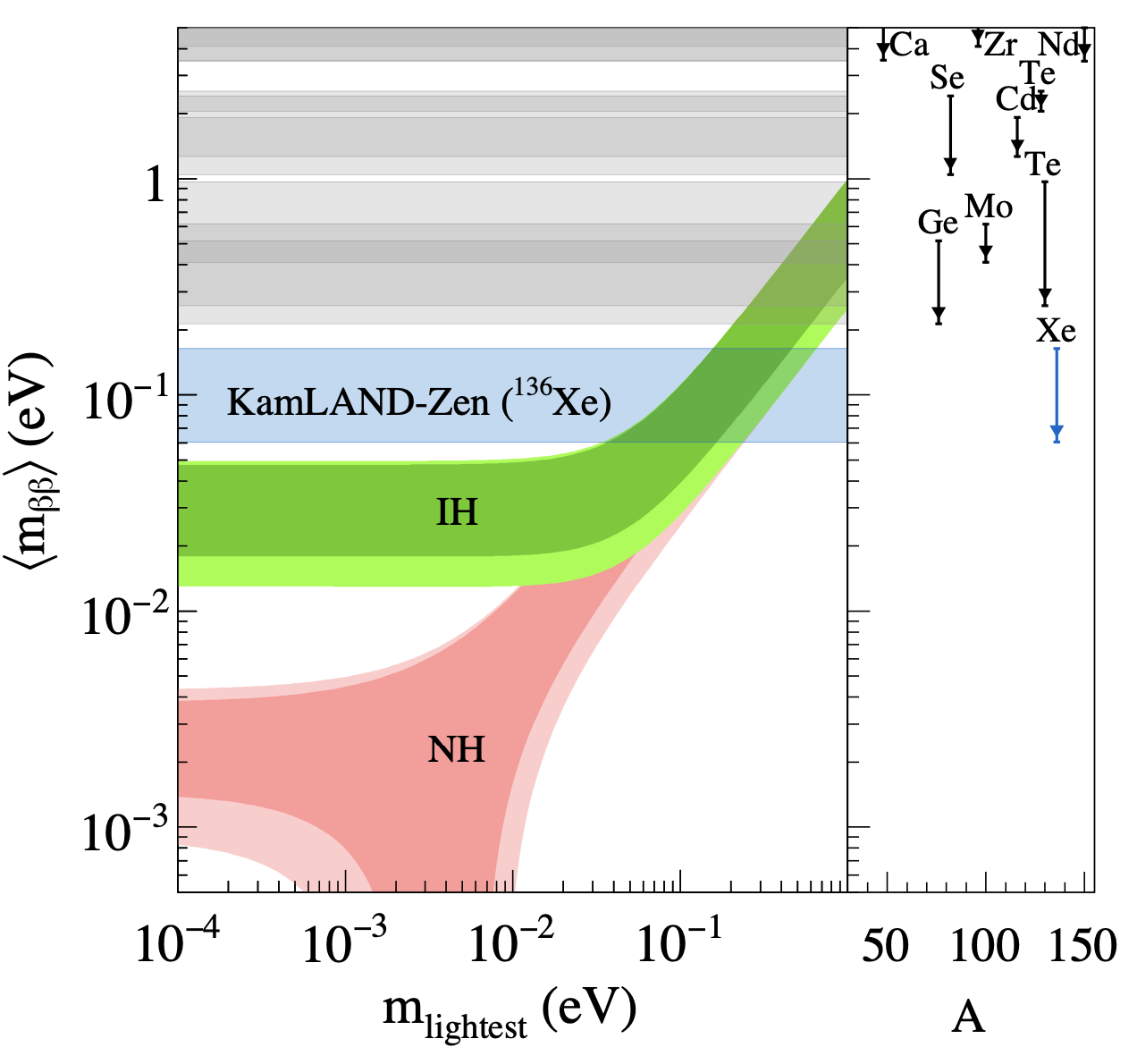
Figure 7: Left: Predictions for the half life of 0nubb in a given reference model with different calculated nuclear matrix elements. Right: Dependence of the parameter $m_{\beta\beta}$ on the presently unknown lightest neutrino mass, with bands showing allowed regions given what is known about mixing parameters.

4.6 The effective Majorana mass

The effective mass that shows up in double beta decay rate of Eq. 71 is a weighted sum of the three neutrinos masses, each contributing proportionally to their probabilistic weight within the electron neutrino flavor state:

$$m_{\beta\beta}=\sum_{i}(U_{ei})^{2}m_{i}.$$ (83)

We can express the matrix elements $U_{ei}$ in terms of the mixing angles and phases that traditionally parameterize the PMNS matrix:

$$U_{\alpha i}=\left[\begin{array}[]{ccc}1&0&0\\ 0&c_{23}&s_{23}\\ 0&-s_{23}&c_{23}\end{array}\right]\left[\begin{array}[]{ccc}c_{13}&0&s_{13}e^{-i\delta}\\ 0&1&0\\ -s_{13}e_{-i\delta}&0&c_{13}\end{array}\right]\left[\begin{array}[]{ccc}c_{12}&s_{12}&0\\ -s_{12}&c_{12}&0\\ 0&0&1\end{array}\right]\left[\begin{array}[]{ccc}e^{i\lambda_{a}}&0&0\\ 0&e^{i\lambda_{b}}&0\\ 0&0&1\end{array}\right]$$ (84)

Multiplying out all the terms in of Eq. 83 then yields:

$$m_{\beta\beta}=c_{12}^{2}c_{13}^{2}e^{2i\lambda_{a}}m_{1}+c_{13}^{2}s_{12}^{2}e^{2i\lambda_{b}}m_{2}+s_{13}^{2}m_{3}.$$ (85)

Let us briefly review what we know about the quantities in this equation [23]. Regarding the neutrino masses, all we know today are the their squared differences, accessed through oscillations. We do not know the absolute mass scale (the lightest $m_{i}$) or whether the observed bigger splitting is between the heaviest two or lightest two neutrinos (the “mass ordering” or “mass hierarchy”). We do know all of the mixing angles, with reasonable precision, from studies of neutrino oscillations between various flavors and on various baselines. We might now know something slightly more than nothing about $\delta_{CP}$ - if we do then this is recent news [24]. We certainly know nothing about the Majorana phases $\lambda_{a}$ and $\lambda_{b}$ since they do not feature in oscillation probabilities, and we have little hope of learning about them, short of observing neutrinoless double beta decay.

In terms of these known and unknown parameters $m_{\beta\beta}$ can be expressed as:

$$m_{\beta\beta}=c_{12}^{2}c_{13}^{2}m_{1}e^{2i\lambda_{a}}+s_{12}^{2}c_{13}^{2}e^{2i\lambda_{b}}\sqrt{m_{1}^{2}+\Delta m_{12}^{2}}+s_{13}^{2}\sqrt{m_{1}^{2}\pm|\Delta m_{23}^{2}|}.$$ (86)

The $\pm$ under the square root of Eq. 86 reflects that at the present time we know the absolute scale of $\Delta m_{23}^{2}$ (from atmospheric and accelerator neutrino experiments) but we do not know its sign (the “mass ordering”, or “mass heirachy”). On the other hand, $\Delta m_{12}^{2}$ is known from solar neutrino oscillation experiments where the MSW effect would drive oscillations differently depending on the relevant ordering, so we do know both its value and sign.

Given the freedom to choose all the unknown parameters $\lambda_{a},\lambda_{b},m_{1}$ in Eq.86, as well as make one discrete choice of the sign of $\Delta m_{23}^{2}$, we find two swathes of allowed decay rates. These bands are commonly represented on what has become colloquially known as “lobster plot” of Fig. 7, right. Here the allowed values for the parameter $m_{\beta\beta}$ featuring in the decay rate (or equivalently the lifetime) is shown with its allowed values plotted against the lightest neutrino mass. The lifetime of neutrinoless double beta decay is proportional to $|m_{\beta\beta}|^{2}$.

5 Mechanisms of neutrinoless double beta decay and the Schechter Valle theorem

We must mention an important point at this juncture. The argument presented so far went as follows: if the known neutrinos are Majorana particles, they will induce neutrinoless double beta decay. This decay will occur at a rate that depends in a well-defined way on $m_{\beta\beta}$, shown in the right plot of Fig. 7. This is true so long as there are three light Majorana neutrinos and no other lepton-number-violating physics that contributes to the decay. Both of these assumptions deserve scrutiny.

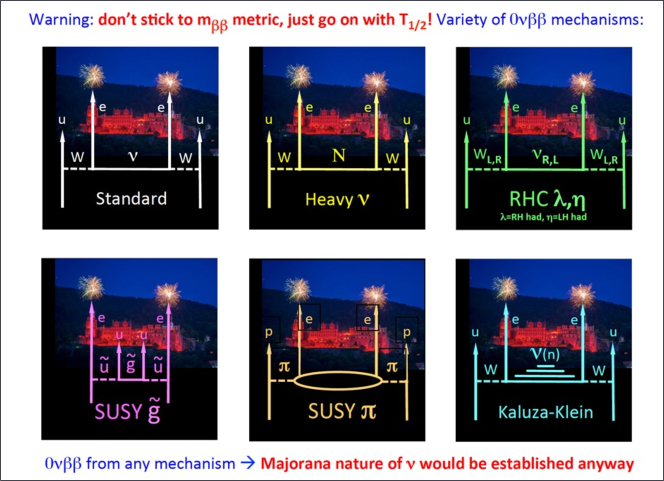
Figure 8: Various mechanisms of $0\nu\beta\beta$, borrowed from  [25].

First, some short baseline experiments have generated anomalies that may be interpreted as evidence of new, heavier neutrino mass states. The corresponding flavor states must be sterile due to constraints from the invisible width of the Z boson [26]. Evidence for sterile neutrinos [27] is presently inconclusive, and there are large tensions between positive and negative observations. Should light sterile neutrinos exist and be Majorana particles they would add an additional mass state to the sum in Eq. 83, invalidating Eq. 86. In the presence of sterile neutrinos, the decay rate may be either much larger or much smaller than the predicted three-neutrino rate in either ordering [28], for a given set of $\lambda_{a},\lambda_{b},m_{1}$, depending on the value of an additional Majorana phase. Existence of a sterile neutrino would move (and widen) the goalposts in neutrinoless double beta decay dramatically.

Furthermore, while light Majorana neutrino exchange may induce neutrinoless double beta decay, it does not necessarily have to be the only mechanism driving the process. There are a wide variety of lepton number violating sources of new physics that may occur within a nucleus and drive $0\nu\beta\beta$. As a fairly general statement, if you have a theory with high scale lepton number violation that introduces effective operators into the low energy Lagrangian at dimension 7, 9, 11, etc [29, 30], there is a good chance it will be able to drive neutrinoless double beta decay. If these more complex mechanisms are responsible for $0\nu\beta\beta$, the relationship between the decay rate and neutrino mixing parameters and masses will, of course, not follow Eq. 75, and could be much larger. This is the case no matter which mass ordering or lightest neutrino mass nature has chosen.

It might seem far-fetched to invoke exotic new physics scenarios as a cause for optimism, to bump up the predicted rate of $0\nu\beta\beta$ above what is suggested by the standard mechanism. It is an especially appealing thing for experimentalists to imagine, especially if we happen to live in a normal-mass-ordered scenario where the lifetimes that must be probed to find the standard mechanism are truly formidable. But is it just wishful thinking, or is there really reason to be hopeful? This is, of course, a question without a truly rigorous answer - but is worth noting that the conventional seesaw mechanism would set the energy scale of neutrino mass generating physics relative to the electroweak scale $\Lambda_{EW}$ at something like $\Lambda_{N}=\Lambda_{EW}^{2}/m_{\nu}\sim 10^{23}\mathrm{eV}$. This is far above the energy scale of most new physics scenarios being sought at (though admittedly not yet found at) the Large Hadron Collider, and many of those scenarios are motivated by the need for TeV-scale physics to resolve the Heirachy problem that leads to quadratic corrections to the Higgs boson mass. Based on purely dimensional arguments, lepton number violation from such lower-scale processes would drive a faster rate of $0\nu\beta\beta$ than the conventional light Majorana neutrino exchange mechanism. Some examples are shown in Fig. 8.

This discussion of the various possible mechanisms may cause one to wonder: if we see $0\nu\beta\beta$, what did we actually learn? If it could be caused by any new physics whatsoever, would we know anything other than “neutrinoless double beta decay happens” if we were to see it? Will we even know the neutrino is a Majorana fermion?

To begin with, we would obviously know right away that lepton number is violated, since we would have observed a lepton number violating process. But it turns out we would know more than this. It turns out that if double beta decay occurs, it is necessary that the neutrino is a Majorana fermion, even if the dominant mechanism causing $0\nu\beta\beta$ were not light Majorana neutrino exchange mechanism we have discussed. The connection is made by the Schechter Valle theorem [31], which says that given any possible source of lepton number violating physics that causes $0\nu\beta\beta$, one can draw a Feynman diagram (Fig. 9) enclosing that new physics as an internal component, whose outcome is the generation of a Majorana neutrino mass. Because of this theorem the logic is bidirectional: existence of Majorana neutrinos implies $0\nu\beta\beta$, if by no other mechanism than at least by light Majorana neutrino exchange; and the existence of $0\nu\beta\beta$ implies Majorana neutrinos masses, generated at least by via Schechter Valle diagram, if nothing else. Observation of $0\nu\beta\beta$ means neutrinos are Majorana; period.

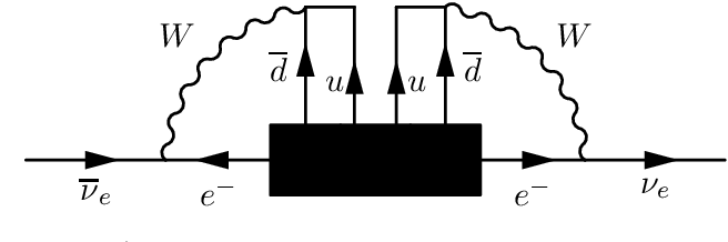
Figure 9: The Schechter Valle Feynman diagram that leads to a Majorana mass, given any new physics that generates $0\nu\beta\beta$

6 Backgrounds and sensitivities to neutrinoless double beta decay

Backgrounds to $0\nu\beta\beta$ only partially derive from the two neutrino process. In experiments that meet the energy resolution criterion $\mathrm{FWHM}\leq 2\%$, backgrounds will generally be dominated by radiogenic processes. These primarily involve gamma rays from the uranium and thorium chains. There is a lot we could say about these backgrounds, about how they can be simulated, minimized, rejected and generally mitigated. For our present purposes, what we need to know is: to have a truly sensitive experiment one must drive these backgrounds down, through either selection of clean materials, use of powerful new technologies, or advanced data analysis methods, to below $B\sim 0.1$ counts per ton per year in the energy region-of-interest, and that is very hard to do.

The reason this is important is shown in Fig. 10, top. This vertical axis of this figure shows the growth in $3\sigma$ discovery potential, defined as the half-life which one would expect to make a $3\sigma$ discovery of in 50% of experimental searches, were the signal real. We can only make this statement statistically since $0\nu\beta\beta$ is a random process and any given nucleus has some probability for decaying and some probability for not decaying while we are looking, no matter how long we wait. The horizontal axis shows exposure, defined as mass times run-time $\epsilon=Mt$: having more of either means more expected signal.

The sensitivities for low exposures are all proportional to $T_{1/2}$. In this low-exposure regime, the number of background events expected is much less than one; thus observation of a single event would be a high-significance a discovery, since it must be signal. Doubling the exposure in this regime effectively doubles the half-life that corresponds to a 50% chance of an event in this time window, explaining the proportionality. Since $T_{1/2}$ is inversely proportional to $m_{\beta\beta}^{2}$, sensitivity of neutrinoless double beta decay experiments initially grows with time as $T_{1/2}\propto\epsilon$, or $m_{\beta\beta}\propto\epsilon^{-1/2}$.

At larger exposures, the lines all transition to being to proportional to $\sqrt{T_{1/2}}$. In this regime the experiment has been running long enough that some background events are expected, and the question becomes one of finding a statistical excess: what is the probability of a given rate of signal events $S$ over particular rate of background. In the high-exposure limit, the number of expected background events $B$ increases proportionally to $\epsilon$, as does the number of expected signal events, so sensitivity grows like $T_{1/2}\propto\sqrt{\epsilon}$, or $m_{\beta\beta}\propto\epsilon^{-1/4}$. When experiments reach this regime their progress in sensitivity is thus exceedingly slow, and returns diminish fast. The determining factor in how soon a given experiment will reach this turning point is the level of background. This is what distinguishes the four curves shown in Fig. 10.

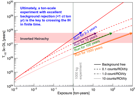
Figure 10: Sensitivity vs background index for neutrinoless double beta decay, adapted from [32].

We see from this figure that to cross the inverted ordering parameter space in reasonable time relies on riding the background-free line as far as possible, with background indices of at most B~0.1, for a ton-scale experiment. We emphasize again though, that this inverted-ordering band is only a visual guide, and discovery of $0\nu\beta\beta$ is in principle possible given either ordering at any value of the half-life beyond existing limits ($10^{26}\mathrm{yr}$ in ${}^{136}Xe$, for example). Once the rate of background becomes comparable to the expected signal, further progress is substantially more difficult. Fig. 11 shows the demonstrated or projected background rate of existing 100kg scale experiments. It is clear that all experiments to date have been in the strongly background limited regime, when extrapolated to ton-scale technologies at their existing levels of background.

The world’s leading experimental limit on $0\nu\beta\beta$ is from the Kamland-Zen experiment [33], which searches for the decay in ¹³⁶Xe-doped liquid scintillator and has set a lifetime limit of $\tau\geq 1.07\times 10^{26}\mathrm{yr}$ at 90% confidence level. This corresponds to a 90% CL upper limit of $m_{\beta\beta}\sim$61-165 meV with the range depending primarily on the nuclear matrix elements assumed. Other, somewhat less strong limits have been obtained using other isotopes including ⁷⁶Ge and ¹³⁰Te. Ongoing R&D now aims to realize lower background technologies for ton- to multi-ton scale experiments.

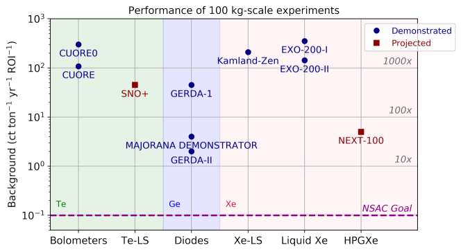
Figure 11: Approximate background indices in present (100kg-scale) programs.

Leading the field in terms of background index at the present time are germanium diodes with $b\sim 2$ counts per ton per year in the energy region of interest, pioneered by the GERDA [34] and Majorana Demonstrator [35] collaborations. The ton-scale phase of these programs is being pursued as a unified international collaboration, via the LEGEND program [36]. Improved background indices beyond the presently demonstrated $b\sim 200$ in liquid xenon from the EXO-200 [37] collaboration are being pursued via the use of dramatic self-shielding of liquid xenon, via the nEXO [38] collaboration, which aims to mount a 5-ton scale liquid xenon time projection chamber, with the goal of improving on the EXO-200 background index by a factor of over 1000. The CUPID [39] collaboration is pursuing a program of development of scintillating bolometers to remove the major background sources from radioactive decays of isotopes plated onto the crystal surfaces in the CUORE tellurium bolometer experiment. And the NEXT collaboration [40] aims to realize a low background high pressure xenon gas time projection chamber at the ton-scale [41], using measurements of both energy and event topology (tracking of two electrons in double beta decay events rather than one from radiogenic backgrounds) to achieve unprecedentedly low background indices with the isotope ¹³⁶Xe. New technologies, including methods of identifying the ¹³⁶Ba ion emitted in the double beta decay of ¹³⁶Xe are also under development [42, 43], which aim for realization of ultra-low-background, or potentially even zero-background technologies at the ton- to multi-ton scale. Fundamental advances such as these are likely to be required in order to penetrate half-lives of the other $10^{28}$ years, as suggested, for example, by the light Majorana neutrino exchange model given a normal neutrino mass ordering.

7 Conclusions

The question of the nature of the neutrino mass is one of profound scientific importance. A discovery of a Majorana nature to the neutrino would confirm the standard model as a low energy effective theory; demonstrate that there are objects in the universe that are neither matter or antimatter but some strange hybrid of the two; illuminate a new mass-generating mechanism for fundamental particles beyond the Higgs mechanism alone; confirm the existence of lepton number violation in nature; and provide support for leptogenesis as the mechanism that generated the observed matter-antimatter asymmetry of the Universe.

Tests of the Majorana nature of the neutrino rely on searching for the hallmark of Majorana neutrinos, lepton number violation, in processes where the neutrinos are intermediate particles that do not need to be directly observed. Achieving sensitivity at high energy accelerator experiments is implausible given what is known about the mass of the neutrino and the chiral properties of the weak interaction. However, an ultimate short-baseline experiment is possible: neutrinoless double beta decay. In this process, exchange of a neutrino between two nucleons in a nucleus leads to production of two electrons and no neutrinos in the final state. If observed, this process would demonstrate the neutrino to be a Majorana particle.

Observation of $0\nu\beta\beta$ is formidably hard, because the process is expected to be extremely slow. However, a range of low-background technologies have been developed that have pursued searches $0\nu\beta\beta$ with sensitivities that have reached beyond $10^{26}$ years in half-life. Now, advanced methodologies and ton- to multi-ton scale experiments are being pursued to push this sensitivity still further, with proposed programs aiming to reach near to $10^{28}$ years in half-life. These experiments are extremely challenging, but the scientific payoff of a discovery would be profound. The quest to discover $0\nu\beta\beta$ continues to motivate an international community of physicists to develop advanced technologies, materials and analysis methods, with the goal of achieving a scientific discovery with profound implications for particle physics, nuclear physics and cosmology.

References

- [1] M. Thomson, Modern particle physics, Cambridge University Press (2013).
- [2] F. Halzen and A.D. Martin, Quark & Leptons: An Introductory Course In Modern Particle Physics, John Wiley & Sons (2008).
- [3] J.J. Gómez-Cadenas, J. Martín-Albo, M. Sorel, P. Ferrario, F. Monrabal, J. Munoz et al., Sense and sensitivity of double beta decay experiments, Journal of Cosmology and Astroparticle Physics 2011 (2011) 007.
- [4] M.J. Dolinski, A.W. Poon and W. Rodejohann, Neutrinoless double-beta decay: status and prospects, Annual Review of Nuclear and Particle Science 69 (2019) 219.
- [5] S.R. Elliott and P. Vogel, Double beta decay, Annual Review of Nuclear and Particle Science 52 (2002) 115.
- [6] W.C. Haxton and G.J. Stephenson, Double beta Decay, Prog. Part. Nucl. Phys. 12 (1984) 409.
- [7] S. Bilenky and C. Giunti, Neutrinoless double-beta decay: A brief review, Modern Physics Letters A 27 (2012) 1230015.
- [8] S. Bilenky and C. Giunti, Neutrinoless double-beta decay: a probe of physics beyond the standard model, International Journal of Modern Physics A 30 (2015) 1530001.
- [9] J. Engel and J. Menéndez, Status and future of nuclear matrix elements for neutrinoless double-beta decay: a review, Reports on Progress in Physics 80 (2017) 046301.
- [10] M.E. Peskin, An introduction to quantum field theory, CRC press (2018).
- [11] S. Weinberg, Baryon-and lepton-nonconserving processes, Physical Review Letters 43 (1979) 1566.
- [12] M. Fukugita and T. Yanagida, Barygenesis without grand unification, Physics Letters B 174 (1986) 45.
- [13] F. Reines and C. Cowan Jr, Detection of the free neutrino, Physical Review 92 (1953) 830.
- [14] M. Aker, K. Altenmüller, M. Arenz, M. Babutzka, J. Barrett, S. Bauer et al., Improved upper limit on the neutrino mass from a direct kinematic method by katrin, Physical review letters 123 (2019) 221802.
- [15] L.-J. Wen, J. Cao and Y.-F. Wang, Reactor neutrino experiments: present and future, Annual Review of Nuclear and Particle Science 67 (2017) 183.
- [16] W. Pauli, On the earlier and more recent history of the neutrino, in Neutrino physics (1991).
- [17] M. Fukugita and T. Yanagida, Physics of Neutrinos: and Application to Astrophysics, Springer Science & Business Media (2013).
- [18] E.J. Konopinski, The Theory of Beta Radio Activity, Clarendon P. (1966).
- [19] J. Kotila and F. Iachello, Phase-space factors for double- decay, Physical Review C 85 (2012) 034316.
- [20] M. Mirea, T. Pahomi and S. Stoica, Values of the phase space factors involved in double beta decay, Romanian reports in Physics 67 (2015) 872.
- [21] H. Ejiri, Neutrino-mass sensitivity and nuclear matrix element for neutrinoless double beta decay, Universe 6 (2020) 225.
- [22] J. Suhonen, Double-beta-decay Matrix Elements and the Effective Value of Weak Axial Coupling, June, 2018. 10.5281/zenodo.1286917.
- [23] G.F. Smoot et al., Review of particle physics, Progress of Theoretical and Experimental Physics (2020) 1.
- [24] K. Abe, R. Akutsu, A. Ali, J. Amey, C. Andreopoulos, L. Anthony et al., Search for c p violation in neutrino and antineutrino oscillations by the t2k experiment with 2.2 10 21 protons on target, Physical review letters 121 (2018) 171802.
- [25] E. Lisi, Opening talk, June, 2018. 10.5281/zenodo.1286745.
- [26] M. Acciarri, O. Adriani, M. Aguilar-Benitez, S. Ahlen, J. Alcaraz, G. Alemanni et al., Determination of the number of light neutrino species from single photon production at lep, Physics Letters B 431 (1998) 199.
- [27] K.N. Abazajian, M. Acero, S. Agarwalla, A. Aguilar-Arevalo, C. Albright, S. Antusch et al., Light sterile neutrinos: a white paper, arXiv preprint arXiv:1204.5379 (2012) .
- [28] C. Giunti and E. Zavanin, Predictions for neutrinoless double-beta decay in the 3+ 1 sterile neutrino scenario, Journal of High Energy Physics 2015 (2015) 1.
- [29] V. Cirigliano, W. Dekens, J. de Vries, M. Graesser and E. Mereghetti, Neutrinoless double beta decay in chiral effective field theory: lepton number violation at dimension seven, Journal of High Energy Physics 2017 (2017) 1.
- [30] V. Cirigliano, W. Dekens, J. de Vries, M.L. Graesser and E. Mereghetti, A neutrinoless double beta decay master formula from effective field theory, Journal of High Energy Physics 2018 (2018) 1.
- [31] J. Schechter and J.W. Valle, Neutrinoless double- decay in su (2) u (1) theories, Physical Review D 25 (1982) 2951.
- [32] M. Agostini, G. Benato and J.A. Detwiler, Discovery probability of next-generation neutrinoless double- decay experiments, Physical Review D 96 (2017) 053001.
- [33] A. Gando, Y. Gando, T. Hachiya, A. Hayashi, S. Hayashida, H. Ikeda et al., Search for majorana neutrinos near the inverted mass hierarchy region with kamland-zen, Physical review letters 117 (2016) 082503.
- [34] M. Agostini, G. Araujo, A. Bakalyarov, M. Balata, I. Barabanov, L. Baudis et al., Final results of gerda on the search for neutrinoless double- decay, Physical Review Letters 125 (2020) 252502.
- [35] C.E. Aalseth, N. Abgrall, E. Aguayo, S. Alvis, M. Amman, I.J. Arnquist et al., Search for neutrinoless double- decay in ge 76 with the majorana demonstrator, Physical review letters 120 (2018) 132502.
- [36] N. Abgrall, A. Abramov, N. Abrosimov, I. Abt, M. Agostini, M. Agartioglu et al., The large enriched germanium experiment for neutrinoless double beta decay (legend), in AIP Conference Proceedings, vol. 1894, p. 020027, AIP Publishing LLC, 2017.
- [37] J. Albert, G. Anton, I. Badhrees, P. Barbeau, R. Bayerlein, D. Beck et al., Search for neutrinoless double-beta decay with the upgraded exo-200 detector, Physical review letters 120 (2018) 072701.
- [38] J. Albert, G. Anton, I. Arnquist, I. Badhrees, P. Barbeau, D. Beck et al., Sensitivity and discovery potential of the proposed nexo experiment to neutrinoless double- decay, Physical Review C 97 (2018) 065503.
- [39] O. Azzolini, M. Barrera, J. Beeman, F. Bellini, M. Beretta, M. Biassoni et al., First result on the neutrinoless double- decay of se 82 with cupid-0, Physical review letters 120 (2018) 232502.
- [40] N. López-March, N. Collaboration et al., Sensitivity of the next-100 detector to neutrinoless double beta decay, in Journal of Physics: Conference Series, vol. 888, p. 012243, IOP Publishing, 2017.
- [41] C. Adams, V. Álvarez, L. Arazi, I. Arnquist, C. Azevedo, K. Bailey et al., Sensitivity of a tonne-scale next detector for neutrinoless double-beta decay searches, Journal of High Energy Physics 2021 (2021) 1.
- [42] C. Chambers, T. Walton, D. Fairbank, A. Craycraft, D.R. Yahne, J. Todd et al., Imaging individual barium atoms in solid xenon for barium tagging in nexo, Nature 569 (2019) 203.
- [43] A. McDonald, B. Jones, D. Nygren, C. Adams, V. Álvarez, C. Azevedo et al., Demonstration of single-barium-ion sensitivity for neutrinoless double-beta decay using single-molecule fluorescence imaging, Physical review letters 120 (2018) 132504.