Flexible rational approximation
and its application for matrix functions

Abstract

This paper proposes a unique optimization approach for estimating the minimax rational approximation and its application for evaluating matrix functions. Our method enables the extension to generalized rational approximations and has the flexibility of adding constraints. In particular, the latter allows us to control specific properties preferred in matrix function evaluation. For example, in the case of a normal matrix, we can guarantee a bound over the condition number of the matrix, which one needs to invert for evaluating the rational matrix function. We demonstrate the efficiency of our approach for several applications of matrix functions based on direct spectrum filtering.

Keywords: matrix functions, minimax approximation, quasiconvex programming.
MSC2020: 15A60; 65F35; 49K35; 65K05; 65K10; 65K15.

1 Introduction

Uniform approximation of functions is considered an early example of an optimization problem with a nonsmooth objective function, providing several textbook examples for convex analysis [43] and semi-infinite programming (SIP) [31]. The natural connections between approximation theory and optimization, both aim at finding the “best” solution, were first forged as interest grew in the application of convex analysis within Functional Analysis in the ’50s, ’60s, and ’70s [16, 24, 39, 40]. In 1972, Laurent published his book [43], where he demonstrated interconnections between approximation and optimization. In particular, he showed that many challenging (Chebyshev) approximation problems could be solved using optimization techniques. For example, one can approximate a nonsmooth function using a piecewise polynomial function (i.e., splines). However, the complexity of the corresponding optimization problems is increased, especially when the location of spline knots (points of switching from one polynomial to another) is unknown. Therefore, in this perspective, rational approximations can be considered a good compromise between approximation accuracy and computational efficiency.

It has been known for several decades [12, 48] that the optimization problems that appeared in rational and generalized rational approximation are quasiconvex (generalized rational approximation in the sense of [48], where the approximations are ratios of linear forms). One of the simplest methods for minimizing quasiconvex functions is the so-called bisection method for quasiconvex optimization [12]. The primary step in the bisection method is solving convex feasibility problems. Some feasibility problems are hard, but there are several efficient methods [6, 78, 79, 80], to name a few. In the case of rational approximation, the feasibility problems we observe in the bisection method can be reduced to solving (large-scaled) linear programming problems and, therefore, can be solved efficiently.

This paper focuses on an optimization approach for the min-max (uniform) approximation. Perhaps surprisingly, we show in [60] that from the optimization perspective, the min-max problem is more tractable than the corresponding least squares. Moreover, the flexibility of our optimization approach allows us to suggest an improved algorithm, which also takes constraints, for example, bounds on the denominator. This property is shown to help apply the approximation for different problems, for instance, evaluating matrix functions.

The term matrix function refers to lifting a scalar function to a matrix domain with matrix values. For a polynomial, such lifting is straightforward since addition and powers are well-defined for square matrices. Otherwise, several standard methods exist to define the lifting mentioned above, e.g., [36, Chapter 1]. Matrix functions have drawn attention in recent years, see e.g., [1, 21, 27, 37, 47, 72], and proved to be an efficient tool in applications such as reduced order models [25, 29], solving ODEs [46], engineering models [22], image denoising [50] and graph neural network [45], just to name a few. For nonsmooth functions, the use of polynomials to evaluate matrix functions is limited due to the nature of polynomial approximation. Therefore, rational approximation, which is also well-defined for matrices, introduces an alternative with much-preferred approximation capabilities [74] and comes with the price of (at least) one inversion. Furthermore, several robust methods for rational approximation have been established in recent years, e.g., [28, 33, 55]. Nevertheless, applying rational approximation for evaluating matrix functions remains a challenging task [30, 54, 77].

In this paper, we show that our rational approximation is especially attractive for evaluating matrix functions where we target the case of normal matrices. In particular, we provide a parameter that controls the matrix’s conditioning and enables a unique trade-off between the ideal uniform approximation and the well-conditioning of the matrix to be inverted in the rational approximation. We describe the algorithm in detail, prove the theoretical guarantee on the conditioning, and demonstrate numerically many aspects regarding the algorithm behavior. In addition, we present an algorithm application for matrix filtering and validate the advantages of our approach.

1.1 Our contribution

This paper focuses on an optimization approach for solving the classic approximation problem of calculating rational min-max approximation. As such, it presents a unique tradeoff, which usually does not appear explicitly in algorithms for calculating rational approximation. In particular, our framework enables adding constraints and calculating the best uniform approximation, which satisfies the required conditions. We compute the rational min-max up to a fixed precision when the constraints are off. Otherwise, we get a rational approximation with some desirable guarantees that best approximate the function up to underlining limitations. In other words, we allow flexibility in the search space of our approximant. The above tradeoff is illustrated numerically for scalar functions but perhaps best demonstrated via the fundamental problem of evaluating matrix functions and some of their applications.

We summarize our main contribution as follows:

1. We present a flexible optimization framework that extends the authors’ previous work includes an improved algorithm, and highlights our ability to determine preferred properties for our rational approximation.

2. The algorithm introduces a novel approach to computing approximation with easy add-ons in the form of constraints, providing a broad base for adjustment for many problems.

3. We offer a unique rational approximation for matrix function, explicitly appealing to evaluate nonsmooth or oscillatory functions.

4. We demonstrate the advantage of our method for matrix function for several applications of matrix spectrum maneuvering.

The paper also supports reproducibility; all source codes and examples are available in an online open repository.

1.2 The structure of the paper

The paper is organized as follows. First, we set the notation and present the problem and several of its state-of-the-art solutions. Then, we introduce the optimization algorithm. We derive the theoretical guarantees, and exhibit the method numerically. Lastly, we discuss several applications to matrix functions, including demonstrations via numerical examples.

2 Problem formulation and prior art

We start by formulating the problem we wish to solve. Then, we proceed with some additional required notation and background.

2.1 Evaluating matrix functions

Matrix function is a result of lifting a scalar function to square matrix domain and with square matrix values (of the same order). In this paper, we mainly focus on the case of real functions of the form $f\colon\mathbb{R}\to\mathbb{R}$, however, this is in general not necessary. Thus, we mostly consider the matrix set consisting of square matrices of size $k\times k$ with real spectrum. When $f$ is a polynomial, such a lifting is straightforward since addition and powers are well-defined for square matrices. When $f$ is not a polynomial, there are several standard methods to define the above-mentioned lifting. If $f$ is analytic having a Taylor expansion whose convergence radius is larger than the spectral radius of a matrix $A$, then the Taylor expansion $f(x)=\sum_{n=0}^{\infty}\alpha_{n}x^{n}$ yields $f(A)=\sum_{n=0}^{\infty}\alpha_{n}A^{n}$. Another elegant definition arises from the Cauchy integral theorem. If $f$ is not analytic, an alternative is defining $f(A)$ on each of the Jordan blocks of $A$ provided that $f\in C^{m-1}$, where $m$ is the size of the largest Jordan block of $A$. For several equivalent definitions, and more details, see e.g. [36, Chapter 1].

Recently, matrix functions received considerable attention, as many essential challenges in their evaluations have been addressed, e.g., [26, 53, 58, 70]. The growing amount of studies in this topic aims to provide modern tools in a vast range of applications. On the classical side, one finds matrix functions in control theory [42]. More theoretic topics, where matrix functions are incorporated, are the solution of differential systems, theoretical particle physics, and nuclear magnetic resonance, see [36, Chapter 2]. Modern applications include complex network analysis [3], graph convolutional neural networks [45], as well as other applications which were mentioned before. Moreover, calculating fundamental matrix functions on specially structured matrices opens the door for many new exciting directions, see, e.g., [72] and references therein.

Our paper suggests a novel algorithm for approximating matrix functions based on rational approximation. The problem we address is defined as follows. Given a real function $f\colon[a,b]\to\mathbb{R}$, and a normal matrix $A$ with all its eigenvalues inside $[a,b]$, construct an approximating matrix $Q$, such that $Q\approx f(A)$. The function is not assumed to be analytic nor smooth. In fact, some fascinating cases consist of merely piecewise smooth functions like the sign, square wave, or absolute value functions. It is worth noting that we may consider $A$ with some of its eigenvalues also in the proximity of $[a,b]$ on the complex plane. In particular, if we set, w.l.o.g, $[a,b]=[-1,1]$ we can allow some extrapolation for eigenvalues in the Bernstein ellipse, that is the ellipse in the complex plane having focal points at the endpoints, $\pm 1$, see [76].

2.2 Uniform rational approximation

Denote by ${\text{P}_{n}}$ the space of polynomials of degree $n$ at the most. The set of type $(m,n)$ rational real functions is defined as ${\text{R}_{{m},{n}}}=\left\{p/q\mid q\in{\text{P}_{m}},\,\,p\in{\text{P}_{n}}\right\}$. A common choice for the parameters is, for example, $(m-1,m)$. When $m=0$, we have that ${\text{R}_{{0},{n}}}={\text{P}_{n}}$.

Over the years, it was a common belief that the power of rational approximation is similar to the one of polynomial. In particular, the rates of convergence or the error bounds are shared between these two families of approximants, see, e.g., [74, Chapter 23]. The absolute value function, while continuous on the interval $[-1,1]$ is not easy to approximate by a polynomial. Specifically, one needs a polynomial of degree $n$ to achieve an error that decays at rate of $\frac{1}{n}$. This error rate is induced by the smoothness of the function and due to the lack of derivative at the origin. In a seminal paper, Newman [57] shows that the error bound, in the case of rational approximation is far superior and reaches a square exponential rate, that is, for a rational approximation of degree $n$ in both denominator and numerator, the error is of order $\exp(-\sqrt{n})$. This result was eventually improved to the asymptotic rate of $8\exp(-\pi\sqrt{n})$ for the rational minimax [71].

Rational approximations, however, can be problematic. There are various computational challenges here, for example, spurious poles, also known as Froissart doublets. These poles-like points introduce a tiny residue and appear when the degrees are chosen to be too large, see [7]. Over the years, various constructions were presented, from the famous Padé approximation which is based on polynomial reproduction, e.g.,  [15, 33] to least-squares techniques [38, 75]. For more general theory of rational approximation, see, e.g., [14] and [74, chapter 23]. In this paper, we take the path of constructing rational approximation via the criterion of uniform approximation error.

Uniform rational approximation for a real function $f$ over a closed segment $[a,b]$ is defined as a minimizer of

$$\min_{r\in{\text{R}_{{m},{n}}}}\max_{x\in[a,b]}\mathinner{\!\left\lvert f(x)-r(x)\right\rvert}.$$ (1)

The approximant is also known as the minimax approximation. The problem (1) is nonconvex and therefore it is challenging even for the existing tools of modern optimization and nonsmooth calculus. There are, however, a number of interesting observations that can be used to approach this problem.

Computationally, attaining the minimax approximation is not an easy task. There are a number of methods, adapted for some types of rational approximation and inspired by the celebrated Remez algorithm [65] originally developed for polynomial approximation. The most promising generalization of this method to the case rational approximations are [5] and [28]. These two adaptations are not suitable for all possible ${\text{R}_{{m},{n}}}$ approximations and therefore more research still needs to be done before applying these approaches. Another possibility is to apply one of the tools of modern nonsmooth calculus [23]. This approach is not very well-known outside of optimization community due to its complexity and technicality. At the same time, it has been successfully applied to free knots polynomial spline approximation problems, that are also very hard due to their nonsmooth and nonconvex nature [73].

Two main methods will serve as a benchmark for testing our rational approximation. The first one is the adaptive Antoulas–Anderson algorithm [55], also known as the AAA algorithm. This method combines two approaches. The first approach is the Antoulas Anderson method [2] representing rational function in a barycentric manner where the user gives the support points. The second approach is to select the support points in a systematic greedy fashion to avoid exponential instabilities. This method does not guarantee optimality in any particular norm. The second method is the Remez algorithm for rational approximation [28, 51], which solves (1) using the equioscillation property.

2.3 Optimization based on quasiconvexity

A function $f\colon\mathbb{R}^{n}\to\mathbb{R}$ is called quasiconvex if

$$f(\lambda x+(1-\lambda)y))\leq\max\{f(x),f(y)\}.$$ (2)

The above (2) is equivalent to saying that the sublevel set of $f$ is convex. Namely, fix $\alpha\in\mathbb{R}$, then

$$S_{\alpha}=\left\{x\in\mathbb{R}^{n}\mid f(x)\leq\alpha\right\},$$ (3)

is a convex set. Quasiconvexity exhibits similar properties to convexity. In particular, $\sup$ and $\max$ operator preserve quasiconvexity while summation does not.

Quasiconvexity was initially introduced by mathematicians working in the area of financial mathematics. The original definition was in terms of sublevel sets and is due to Bruno de Finetti [20]. The term quasiconvexity appeared much later. Modern studies of quasiconvexity and quasiconvex optimization include [17, 19, 49, 56, 66, 67, 68].

Quasiconvex problem (with or without linear constraints) can be treated using computational methods developed for quasiconvex optimization [12, 49, 56]. In this paper we use the bisection method for quasiconvex functions. This is one of the simplest quasiconvex optimization method, but it is very efficient and includes linear constraints in a very natural way, which is especially important for our applications. The description of this method can be found, for example, in [12]. The main difficulty of this method is to formulate and solve the so called convex feasibility problems. These problems may be hard [6], but additional linear constraints do not affect the complexity. Since our applications only require additional linear constraints, this method can handle such applications well. We will discuss this issue in the next section.

2.4 Bisection method for quasiconvex optimization

Bisection method is a simple and reliable quasiconvex optimization method, see [12, Section 4.2.5] for more information. In all the examples in this paper, the corresponding convex feasibility problems (discrete case) can be reduced to solving linear programming problems when the space is finite, while for the continuous case the convex feasibility problems are linear semi-infinite. More information on linear semi-infinite problems can be found in [32].

Consider a quasiconvex optimization problem with linear constraints:

$${\rm minimize}~{}\phi(x)$$ (4)

subject to

$$Mx\leq b,$$ (5)

where $\phi(x)$ is a bounded quasiconvex function, $x\in X\subset\mathbb{R}^{d}$, $X$ is a convex set. Constraints (5) are linear equations and inequalities. The set, let us call it $C$, of feasible points satisfying these constraints is convex, that is, the set $C$ is nonempty. Fix $z$, the sublevel set $\phi_{z}=\{z\mathrel{\mathop{\mathchar 58\relax}}\phi(x)\leq z\}$ is convex, since $\phi$ is quasiconvex.

The set $C_{z}=C\cap\phi_{z}$ is convex as the intersection of two convex sets. Assume that problem (4)-(5) is feasible, that is, constraints (5) are consistent. Then,

• if $C_{z}$ is empty, then the optimal value for (4)-(5) is strictly higher than $z$;

• if $C_{z}$ is not empty, then the optimal value for (4)-(5) does not exceed $z$.

The procedure of checking whether set $C_{z}$ is empty or not is called convex feasibility. In the next section we will demonstrate that in our problems this procedure can be reduced to solving a linear programming problem and therefore it can be solved fast and efficiently.

Note that feasibility problems aim at finding a feasible point in a given set of constraints and therefore this point is not necessarily an optimal solution for some objective function associated with this set of constraints, but in most cases feasibility problems are formulated as optimization problems. In general, these problems may be very hard to solve, but there are a number of efficient methods, see, e.g., [6, 78, 79, 80, 82]. There are still many open problems in this area.

It was noticed long time ago that rational and generalized rational approximation problems can be solved by fixing the level set of the objective function at some value and then solve linear programming problems, see for example [52, 64]. Later it was demonstrated that these problems can be formulated as optimization problems with linear objectives and quasiaffine constraints (see section 3 of this paper for details and references). Therefore they belong to the class of quasiconvex optimization problems and can be solved using quasiconvex optimization methods (for example, bisection). Moreover, some earlier developed methods are implementations of bisection method for quasiconvex functions [61]. It was demonstrated in [67] that the sublevel sets of quasiaffine functions are half-spaces and therefore the constraint sets in the corresponding optimization problems are polyhedra, but there is no approach for constructing these polyhedra for general quasiaffine constraints. However, in the case of rational and generalized rational approximation we do know how to construct the polyhedra and the idea is coming from the early works mentioned above. More details in section 3. This problem is a beautiful example of interconnections between modern optimization techniques and classical approximation results obtained in the 60-70s of the twentieth century.

Algorithm 1 Bisection algorithm for quasiconvex optimization with linear constraints

0:  Maximal deviation $z$ (within $\varepsilon$ precision). Start with given precision $\varepsilon>0$.

  set $l\leftarrow 0$

  set $u$

  $z\leftarrow(u+l)/2$

  while $u-l\leq\varepsilon$ do

     Check if $C_{z}$ is empty.

     if feasible solution exists ($C_{z}$ is not empty) then

        $u\leftarrow z$

     else

        $l\leftarrow z$

     end if

     update $z\leftarrow(u+l)/2$

  end while

The bisection method which we use is given in Algorithm 1. It is essential for Algorithm 1 to start with tight upper bound $u$ and lower bound $l$. Since our quasiconvex function corresponds to the maximal absolute deviation between original function $f$ on $[a,b]$ (multivariate generalization are also possible) and its approximation, the lower bound $l$ can be set as zero (that is, $l\leftarrow 0$). The upper bound $u$ can be set as $u=\frac{1}{2}(\max f(x)-\min f(x))$.

Note that at each iteration of the bisection algorithm the length of the search interval is halved, meaning that it takes at most $\log_{2}(\nicefrac{{L}}{{\varepsilon}})$ steps to reach a solution within the desired accuracy $\varepsilon$. When approximating the function over a discrete set of points, the convex feasibility problem can be solved with a polynomial-time algorithm for linear programming (such as Karmarkar’s method [41] for example), and the proposed algorithm reaches an approximate solution in polynomial time.

3 Flexible uniform rational approximation via optimization

This section describes in details the construction of our optimization algorithm. This algorithm serves as an improved version of the method presented in [60]. Here, we focus on a specific instance of rational approximation with further constraints and guarantees.

3.1 Optimizing a rational approximation

3.1.1 Quasiconvexity and the optimization setup

The goal of our optimization method is to solve (1). We therefore denote our approximation by

$$r(x)=\frac{\alpha^{T}\mathcal{G}(x)}{\beta^{T}\mathcal{H}(x)},\quad\text{subject to}\quad\beta^{T}\mathcal{H}(x)>0,\quad\mathcal{H}\in\left({\text{P}_{m}}\right)^{m+1},\quad\mathcal{G}\in\left({\text{P}_{n}}\right)^{n+1},$$ (6)

where $\mathcal{H}$ and $\mathcal{G}$ are basis vectorized functions, $\alpha\in\mathbb{R}^{n+1}$ and $\beta\in\mathbb{R}^{m+1}$ are the decision variables, $({\text{P}_{k}})^{k+1}$, $k=\{n,m\}$ are $(k+1)$-dimensional vectors, whose components are the monomials of degree at most $k$. The components of $({\text{P}_{k}})^{k+1},~{}k=\{n,m\}$ are also called the basis functions. We can use the same formalization to define a generalized rational function: it is enough to replace the basis functions by other Chebyshev systems of the same dimension, for example, exponential functions. In this paper, we focus on polynomials and use as our basis functions the Chebyshev polynomials of the first kind, as defined in (18). For more technical details on these polynomials, see A.

At this point, it is worth rewriting (1) in terms of (6) to have

$$\min_{\begin{subarray}{c}\alpha\in\mathbb{R}^{n+1}\\ \beta\in\mathbb{R}^{m+1}\end{subarray}}\max_{x\in[a,b]}\mathinner{\!\left\lvert f(x)-\frac{\alpha^{T}\mathcal{G}(x)}{\beta^{T}\mathcal{H}(x)}\right\rvert},$$ (7)

subject to

$$\beta^{T}\mathcal{H}(x)>0,\quad x\in[a,b].$$ (8)

It has been proved in [48, Lemma 2] that the objective function of (7) is quasiconvex. This important result was not considered as essential for [48] and therefore was obtained as an intermediate result and was hidden for some decades. A simpler proof of this result can be found in [12, 60]. Thus, in light of (3), the problem (7)-(8) has an optimal solution for any fixed, large enough (larger than the minimax uniform error), upper bound.

3.1.2 Bisection method and convex feasibility problem

In practice, we solve the problem for discrete set of points $\{x_{i}\}_{i=1}^{N}\subset[a,b]$ where $N\geq m+n+2$. Namely, we search for a minimal $z$ that solves

$$f(x_{i})-\frac{\alpha^{T}\mathcal{G}(x_{i})}{\beta^{T}\mathcal{H}(x_{i})}\leq z\quad\text{and}\quad\frac{\alpha^{T}\mathcal{G}(x_{i})}{\beta^{T}\mathcal{H}(x_{i})}-f(x_{i})\leq z,$$ (9)

with the constraint

$$\beta^{T}\mathcal{H}(x_{i})>0.$$ (10)

To obtain the corresponding sublevel set, fix $z$ for (9), then the sublevel set is described as (9)-(10). Note that when $z$ is fixed, all the constraints are linear and the convex feasibility problem is reduced to finding a point from this polyhedron. This can be done by solving the following linear programming problem:

$$\min(\theta)$$

subjects to

$$(f(x_{i})-z)\beta^{T}H(x_{i})-\alpha^{T}\mathcal{G}(x_{i})\leq\theta$$ (11)

$$\alpha^{T}\mathcal{G}(x_{i})-(f(x_{i})-z)\beta^{T}\mathcal{H}(x_{i})\leq\theta$$ (12)

$$\beta^{T}\mathcal{H}(x_{i})\geq\delta,$$ (13)

where $\delta$ is a small positive number. The feasibility problem has a solution if and only if $\theta\leq 0$.

Remark 1.

Note that as the number of available points $N$ grows, we obtain more information about approximating the function. However, as $N$ gets larger, so are the required computational resources and runtime of any optimization algorithm that we may employ. Therefore, ideally, we wish to keep $N$ small while extracting enough information so the rational approximation will be as accurate as possible.

Sampling a function is the subject of numerous studies, e.g., [81], which is beyond the scope of this paper. In practice, one can use a global sampling strategy, for example, equidistant sampling, which is sufficient in many cases (as seen in the sequel). Furthermore, a universal approach for a wide class of common functions is introduced in [4], which randomly samples the segment of interest according to non-uniform ideal sampling distribution. Alternatively, when the number of points is required to be small, one may use Chebyshev points (or nodes) which are the roots of the Chebyshev polynomial of the first kind. The Chebyshev points are particularly beneficial when utilizing Chebyshev polynomials as the basis functions due to the discrete orthogonality (24).

Remark 2.

The bisection technique is merely a straightforward option for solving the above optimization problems. The main advantage, apart of being simple, is that it guarantees precision. Nevertheless, several more efficient methods may be applied here, for example [59]. Yet, when keeping matrix functions as our top motivational application, it is clear that the bulk of computation efforts is devoted to forming matrix polynomial and inverting a matrix. Therefore, in this perspective, the efficiency of the method we employ is marginal, and the benefits of the bisection remain significant. In particular, the bisection method is straightforward if one needs to add linear constraints. More work may be required if the additional constraints are convex, quasiaffine (quasilinear) or quasiconvex, but the sets appearing in feasibility problems in the bisection method remain convex, since they represent sublevel sets of quasiconvex functions.

This research direction has many practical applications and is one of our future research directions and in particular is the study of possibility to include non-linear constraints. One simple example that illustrated a possibility to deal with quasiconvex constraints can be found in [61].

3.2 Denominator Bounds

A critical stage in evaluating matrix function via rational approximation of the form $r(x)=p(x)/q(x)$ is to invert the resulting denominator, that is to calculate $q(A)^{-1}$. Thus, we suggest to add a constraint for bounding (10) as,

$$0<\ell\leq\beta^{T}\mathcal{H}(x_{i})\leq u.$$ (14)

For what follows, we denote the condition number of a matrix $X$ with respect to the matrix $2$-norm by $\operatorname{cond}\left(X\right))=\mathinner{\!\left\lVert X\right\rVert}_{2}\mathinner{\!\left\lVert X^{-1}\right\rVert}_{2}$ and by $\lambda_{\min}(X)$ and $\lambda_{\max}(X)$ the minimal and maximal eigenvalue, possibly complex, of a real matrix $X$, when measured in absolute value. The next theorem shows that bounding the denominator of our approximant from both sides as in (14) keeps the condition number of the resulted denominator bounded as well.

Theorem 1.

Let $r=\dfrac{p}{q}\in{\text{R}_{{m},{n}}}$ and assume that

$$0<\ell\leq\mathinner{\!\left\lvert q(x)\right\rvert}\leq u,\quad x\in\Omega.$$

Furthermore, assume $A$ is a real normal matrix with all eigenvalues in $\Omega$. Then,

$$\operatorname{cond}\left(q(A)\right))\leq u/{\ell},$$

Proof.

Denote by $\{\lambda_{j}\}_{j=1}^{k}$ the eigenvalues of $A$. Then, the eigenvalues of $q(A)$ are $\{q(\lambda_{j})\}_{j=1}^{k}$ and so,

$$\mathinner{\!\left\lVert q(A)\right\rVert}_{2}=\max_{\lambda_{j}}\mathinner{\!\left\lvert q(\lambda_{j})\right\rvert}\quad\text{and}\quad\mathinner{\!\left\lVert q(A)^{-1}\right\rVert}_{2}=1/\min_{\lambda_{j}}\mathinner{\!\left\lvert q(\lambda_{j})\right\rvert}.$$

Thus, by the bounds on $q$ over $\Omega$ we deduce that

$$\operatorname{cond}\left(q(A)\right))\leq\mathinner{\!\left\lVert q(A)\right\rVert}_{2}\mathinner{\!\left\lVert q(A)^{-1}\right\rVert}_{2}\leq u/\ell.$$

∎

The above Theorem 1 implies that adding bounds on the denominator, when optimizing for the best rational approximation, results in a matrix $q(A)$ with a bounded condition number, regardless of the distribution of eigenvalues of $A$. The condition number of $q(A)$ is particularly important since this is the matrix we need to invert for evaluating the matrix function $r(A)$ .

3.3 Numerical performance of the optimization method

We conclude this section with several demonstrations of the rational approximation as obtained by our optimization algorithm. Specifically, we consider four test functions, investigate the effect of the different parameters, and compare our approximation with the output of the Remez algorithm, as implemented in [59] and the AAA algorithm from [55].

A few technical details about the algorithms and test settings. For the optimization algorithm, we set the parameter of bisection accuracy for the optimization to $10^{-15}$ and use $400$ equidistant points over the relevant segment. The AAA algorithm gets the same set of points for a fair comparison, while the Remez algorithm gets a function handler and access to any value of the function. The reason for the latter is that we want to compare the error rates with what we get from one of the minimax solutions, as obtained in ideal settings. Once all approximations are calculated, we evaluate them at the same $1000$ points, distributed uniformly over the segment. We then report the maximum absolute deviation from the original function as the uniform error. The entire source code, including all test parameters, is available at  https://github.com/nirsharon/RationalMatrixFunctions.

The set of test functions we use consists of a cubic spline function, a function with a cusp, an oscillatory function, and the absolute value function. We present the test functions in Table 1. The table includes the domain where we approximate the function and the fundamental parameters for our optimization algorithm: the degrees of the rational approximation $(m,n)$ and the denominator upper bound $u$ of (14) where the lower bound is fixed at $\ell=1$. The test functions differ not only by their domain but mainly by their smoothness level, as reflected by the characteristics of their derivatives. In particular, the spline $f_{1}$ has a jump discontinuity at the third derivative. The cusp function $f_{2}$ has a stronger asymptotic discontinuity at its first derivative, and the oscillatory function $f_{3}$ has a rapidly changing derivative. The shifted absolute value $f_{4}$ has a jump discontinuity at the first derivative.

Test function	$[a,b]$	$(m,n)$	$u$ of (14)
$f_{1}(x)=\begin{cases}-x^{3}+6x^{2}-6x+2&x<1\\ x^{3}&1\leq x\\ \end{cases}$	$[0,3]$	$(m-1,m)$	2,4,8,100
$f_{2}(x)=\mathinner{\!\left\lvert x\right\rvert}^{2/3}$	$[-1,2]$	$(6,6)$	100
$f_{3}(x)=\cos{9x}+\sin{11x}$	$[-1,1]$	$(7,7)$	50
$f_{4}(x)=\mathinner{\!\left\lvert x-0.1\right\rvert}$	$[-0.5,0.5]$	$(6,6)$	100

Table 1: The test functions, their domains and the parameters that we use for constructing their rational approximation

Following Section 3.2, we give a special focus for the denominator of each approximation, since, by Theorem 1, it implies how suitable the approximation is for matrices. In particular, we measure the maximum absolute change in the denominator values of a rational function $r(x)=p(x)/q(x)$ over $[a,b]$, denoted by

$$C_{r}=\max_{x\in[a,b]}\mathinner{\!\left\lvert q(x)\right\rvert}/\min_{x\in[a,b]}\mathinner{\!\left\lvert q(x)\right\rvert}.$$ (15)

This value indicates how high the condition number of $q(A)$ may be, for a given matrix $A$ with eigenvalues inside $[a,b]$.

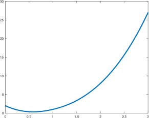
Figure 1: $f_{1}$ over $[0,3]$

We use $f_{1}$, as it appears in Figure 1, and test the effect of changing the denominator upper bound $u$ of (14). We use rational approximations of type $(4,5)$, relatively small degrees, which are sufficient for obtaining uniform error rates of about $0.0009$ via the Remez algorithm and $0.0025$ using (5,5) AAA approximation (the implementation of AAA cannot have $n\neq m$). First, we choose a restrictive $u=2$. This value guarantees that $C_{r}$ of (15) for the optimization approximant will be no bigger than $2$, and so is the condition number of any denominator matrix evaluation. The error rates of this case appear in Figure 2(a). Our optimization method yields an approximation with a uniform error of $0.0051$. This rate is two times higher than the AAA one, as seen in the figure. However, by increasing $u$, we allow a larger search space for the optimization, and $u=4$ is already enough for obtaining a slightly better approximation than the AAA, as seen in Figure 2(b). The AAA denominator satisfies $C_{r}=3.91$. So it is inside the search space of the optimization, which explains how we have been able to find a better approximation in terms of uniform error. Lastly, we set $u=8$. In this case, as seen in Figure 2(c), the optimization successfully recovers a minimax approximation with a uniform error of $0.0009$, as obtained by the Remez algorithm. Indeed, both the Remez and our method approximation introduce the same $C_{r}=6.86$, which lies within the constraint range.

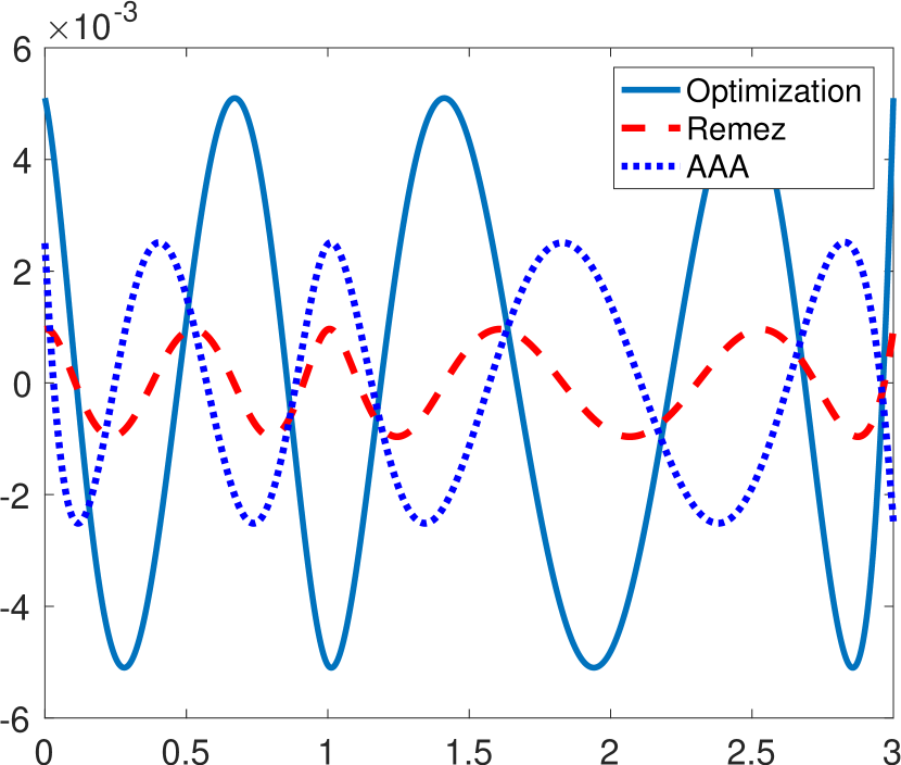
(a) $u=2$

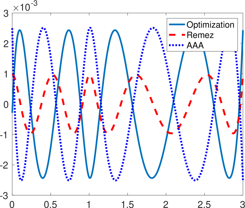
(b) $u=4$

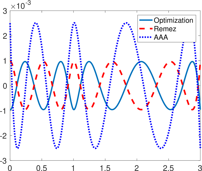
(c) $u=8$

Figure 2: The effect of changing denominator bounds with fixed degrees. We set the rational polynomial degrees to (4,5) and compare our method with the (5,5) AAA and (4,5) Remez approximations. On the left, the upper bound $u$ of (14) is $2$, and the resulted approximation is nonoptimal. Then, as the bound increases to $4$, so is the accuracy of the optimization output. Finally, we recover a minimax rational approximation when setting $u=8$ (on the right). This series of examples illustrates the tradeoff between the denominator bound and the ability to achieve optimal approximation.

In the next test, we further examine our method using $f_{1}$ as a test function, but now fixing $u$ of (14) to be $100$. On the other hand, we let the degrees $m$ of the $(m-1,m)$ approximations to vary from $5$ to $11$. The resulted error rates and absolute denominator change are presented together in Figure 3. The results show that when $u$ is large enough to enable the minimax, the optimization establishes such an approximation. Nevertheless, as the degree increases, the bound for the denominator becomes more restrictive, and the error rates decay a bit slower than the ones of the minimax. Notwithstanding this, the difference in denominator absolute change of the two rational approximations rises dramatically with the degree.

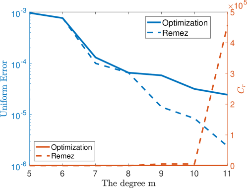
Figure 3: Error rates and denominator absolute change $C_{r}$ of (15) as functions of the degrees. We set $u$ of (14) to $100$ and compare the outputs of our method with the minimax approximations as calculated by the Remez algorithm. While $u$ is smaller than $C_{r}$ of the minimax, the error rates are similar. As degree grows, the $C_{r}$ of Remez increases dramatically. This growth introduces a tradeoff between bounding the $C_{r}$ and increasing the approximation precision

We conclude this section with several snapshots of error rates and absolute denominator changes for the other three test functions. These examples further illustrate the trade-off between accurate approximation and bounding the denominator change, for different functions, with distinct characteristics. In particular, it also shows the performance of other rational approximation (AAA) and the high price tag of attaining a high-precision approximation — expressed as a high $C_{r}$ value. The results are depicted in Figure 4 where we present each test function alongside the error rates of the three methods (optimization, AAA, and Remez) and the resulted denominator polynomial of each approximation. In addition, we mention the uniform error rates and the values $C_{r}$ of (15) as obtained by each method.

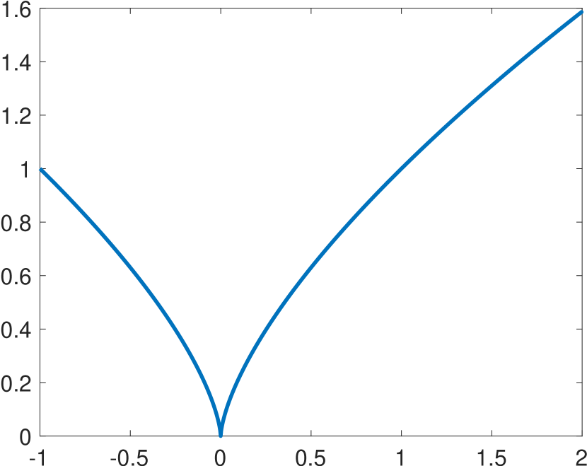
$f_{2}$ over $[-1,2]$

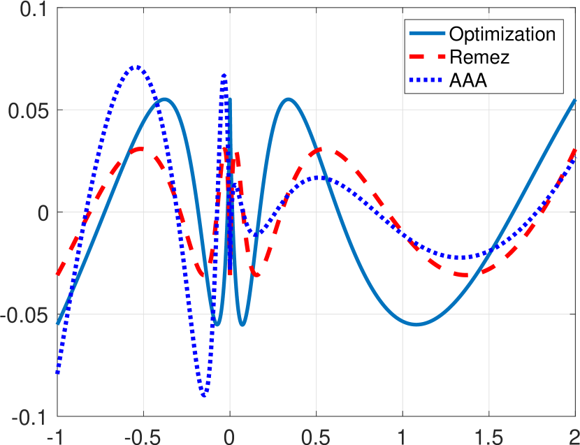
Errors: $0.055$, $0.030$, $0.089$

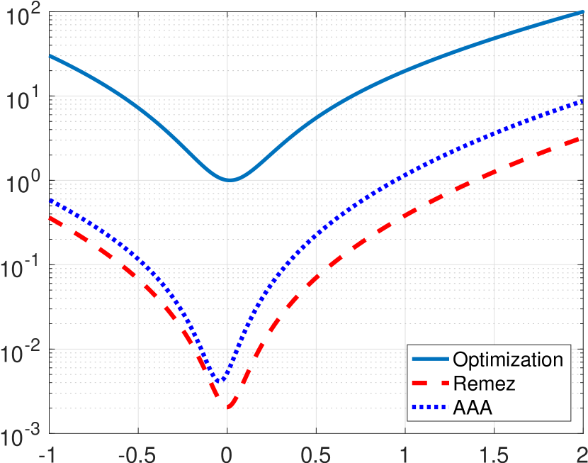
$C_{r}$: $100$, $1571$, $2096$

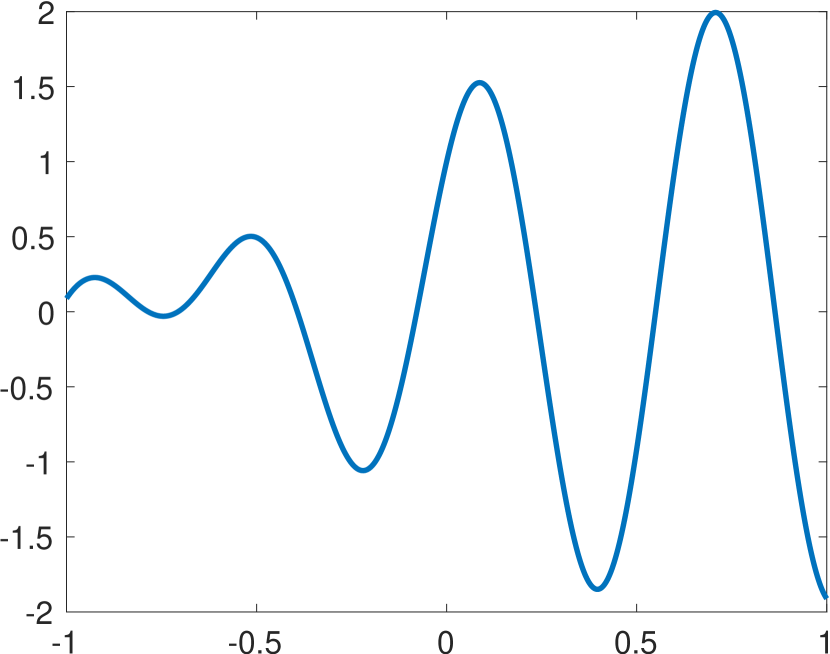
$f_{3}$ over $[-1,1]$

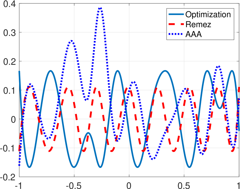
Errors: $0.167$, $0.111$, $0.386$

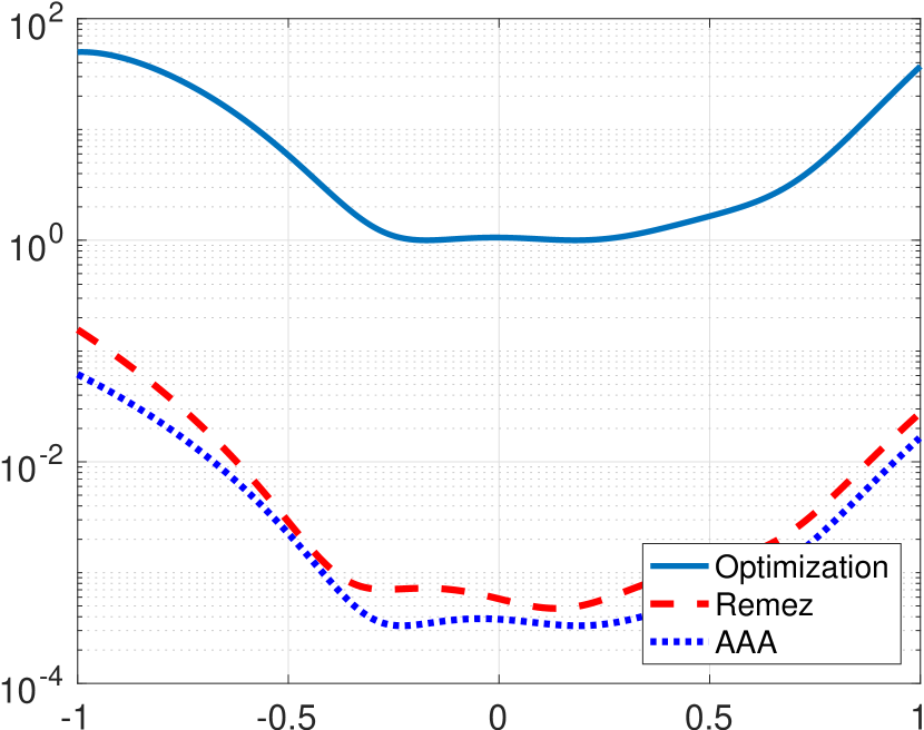
$C_{r}$: $50$, $327$, $185$

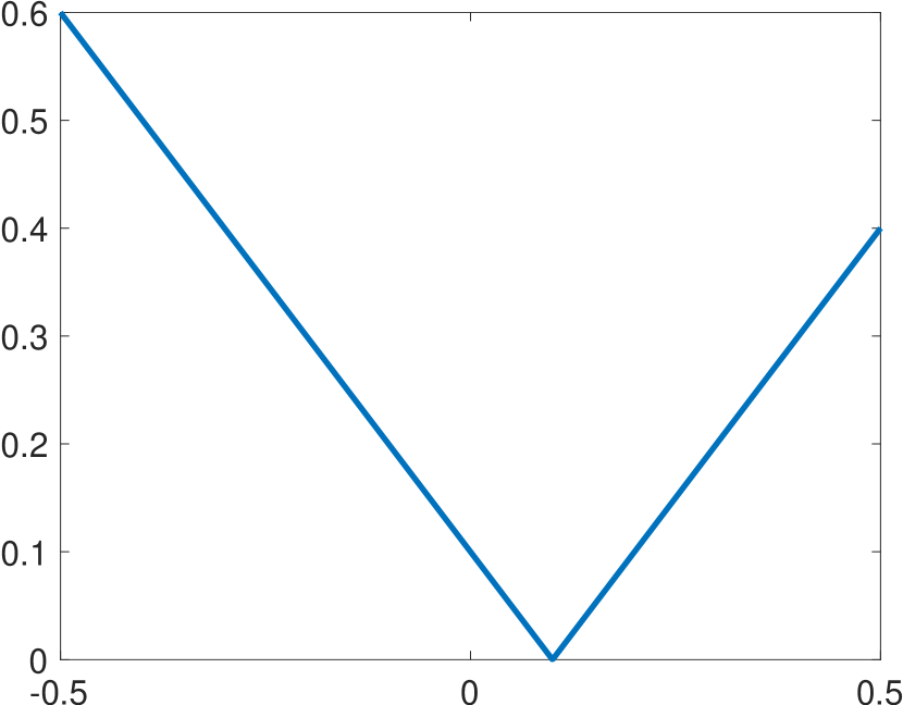
$f_{4}$ over $[-0.5,0.5]$

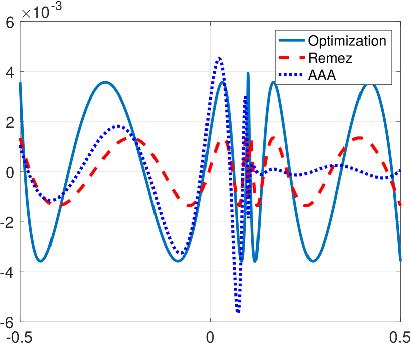
Errors: $0.0039$, $0.0013$, $0.0056$

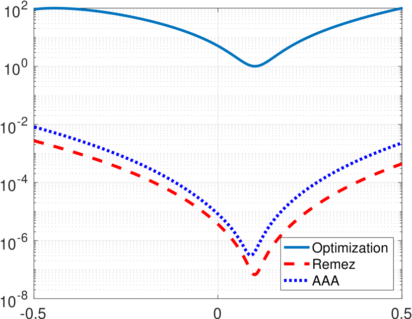
$C_{r}$: $100$, $40,504$, $26,101$

Figure 4: Comparison of the three methods for rational approximation — optimization, Remez, and AAA, using the three test functions $f_{2}$ to $f_{4}$, see Table 1. On the left are the test functions, in the middle column are the error rates, which are reported together with the uniform errors. On the right, the denominator polynomials of the three rational approximations and their associated value $C_{r}$ of (15). The reported values are of the above order (optimization, Remez, AAA)

4 Approximating matrix functions

The notable advantage of rational approximations over polynomials in scalars motivates us to apply it for matrix functions. Calculating rational matrix functions includes several challenges, see for example [54]. However, since matrix polynomials are well understood, the main bottleneck is evaluating the denominator polynomial, which means inverting a matrix polynomial. Two main issues lie in this denominator evaluation. The first is the expensive computational cost. Second, and perhaps more severe in certain situations, is the condition number of the matrix to be inverted. A high condition number indicates the inversion is ill-posed, and the matrix function approximation will contain significant errors. Our general approach for evaluating matrix functions vis scalar rational approximation is illustrated in a diagram on Figure 5.

Figure 5: Illustration of approximating matrix function via scalar rational approximation.

In the following, we introduce two applications of our rational approximation for two different tasks of matrix evaluation. The first one is filtering the spectrum of a given matrix, also known as spectrum slicing. The second one is projecting a symmetric matrix to the cone of positive semidefinite matrices. For both applications, the goal is to introduce an alternative solution that does not explicitly recover the spectral structure of the given matrix. Instead, we design a suitable function and lift it to obtain the desired matrix function.

As in previous section, the entire source code, including all test parameters, is available at  https://github.com/nirsharon/RationalMatrixFunctions. We ran the tests on a 2.9 GHz Dual-Core Intel Core i5 processor with 16 GB RAM using a macOS operation system and Matlab 2017b.

4.1 Spectrum filtering of a matrix

The power method is a classical algorithm to extract the leading eigenvalue of a matrix. Its variants and modern versions appear in many applications and areas of science and engineering. When the eigenvalue we wish to recover is not the largest in magnitude, we can use the inverse power method technique and search for the largest eigenvalue of $(A-\alpha I)^{-1}$ where $\alpha$ is a value close to the required eigenvalue, see, e.g., [69]. Nevertheless, when the spectrum is unknown, and we wish to preserve or manipulate only a subset of the eigenvalues, we need to reveal it extensively. Such direct methods may be costly and, in general, do not scale well. An alternative approach is to filter the spectrum implicitly by lifting it using a matrix function. This ideal was used for spectrum slicing, see, e.g., [8, 47], but can be applied for various broad areas of applications such as improving covariance estimation via shrinkage [44] or optimizing risk factors in financial portfolios [10], just to name a few.

In the next example, we assume that the eigenvalues of a given matrix are real and bounded in absolute value by $1$. The goal is to retain only the eigenvalues at a certain subsegment of $[-1,1]$. In this example, we choose the segment around $0.4$ at radius $0.15$, that is $[0.25,0.55]$. For this task, the ideal filter to be applied on the spectrum is $H(x)=x(h(x-0.25)-h(x-0.55))$ where $h(x)$ is the Heaviside step function. However, this function is not even continuous and so we use a smoother version of it,

$$F(x)=\frac{x}{2}\left(1-\operatorname{erf}(2(\nicefrac{{\mathinner{\!\left\lvert x-c\right\rvert}}}{{r}})-R)\right).$$ (16)

Here, $\operatorname{erf}$ is the Gauss error function, $c=0.4$ is the center of the segment, R = 0.2 is the width (radius), and $r=0.05$ determines the rise rate from zero. This function is continuous with a single jump discontinuity at the first derivative (due to the absolute value). The function, the particular segment where we want the eigenvalues to be preserved, and the ideal filter described above are presented in Figure 6.

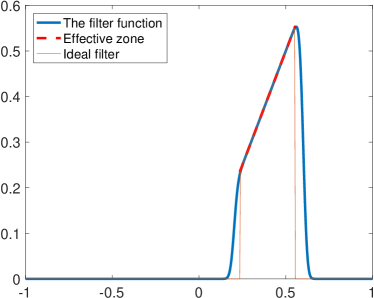
Figure 6: The filter function $F$ of (16). The effective zone of eigenvalue preservation, $[0.25,0.55]$, is marked, together with the corresponding ideal filter function

We approximate $F$ of (16) using three functions: the output of our optimization, the AAA rational approximation, and the minimax polynomial, as obtained by the Remez algorithm. The two rational approximations are of type $(10,10)$ and the polynomial is of degree $20$. Figure 7 presents the approximations, and in particular, Figure 7(a) shows the functions. In Figure 7(b) we present the corresponding error rates, which in uniform norm are $0.0083$, $0.0062$, and $0.0948$ for the optimization, AAA, and Remez’s polynomial, respectively. For our optimization, we set the upper bound $u$ of (14) to be $1000$. The AAA approximation, on the other hand, introduces $C_{r}$ value of about $2.6\times 10^{9}$. The two denominators are depicted in Figure 7(c). As we will see next, the huge change in the denominator of the AAA approximation plays a significant role when applying the rational approximation to matrices.

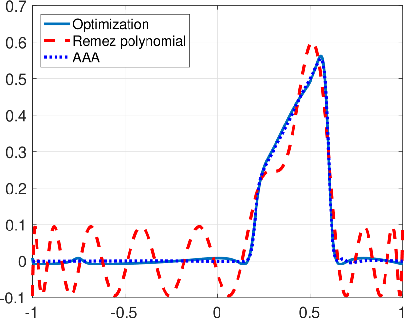
(a) The approximations: $(10,10)$ rational approximations based on our method of optimization and of AAA, and a $(20)$ degree minimax polynomial obtained by the Remez algorithm

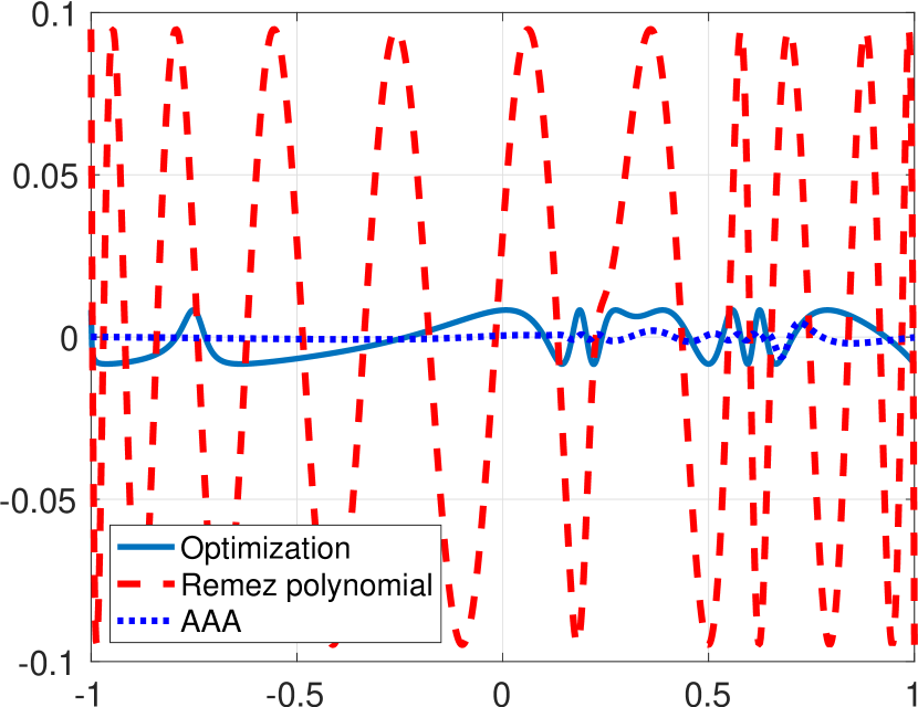
(b) The error rates. In uniform norm the errors are $0.0083$, $0.0062$, and $0.0948$ for the optimization, AAA, and Remez’s polynomial, respectively

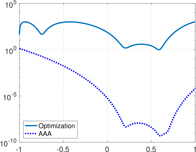
(c) The denominators of the rational approximations. Overall change value $C_{r}$ of (15) is $1000$ and $2.6\times 10^{9}$ for the optimization and AAA, respectively

Figure 7: The approximation of the filter function $F$ of (16)

As the approximations are established, we proceed and apply them on a matrix. We construct a $100\times 100$ matrix as follows: we randomly select an orthogonal matrix $Q$ and use a diagonal matrix $D$ with Chebyshev nodes as its diagonal values. Then we form $A=QDQ^{\ast}$ and $F(A)=QF(D)Q^{\ast}$ where $F$ is the function (16) and $F(D)$ is understood as applying the function on the diagonal element-wise. Each of the above approximations for $F$ will approximate $F(A)$ when applied to $A$. Both spectra of $A$ and $F(A)$ are presented in Figure 8.

For each approximation $s$ of $F$, we measure its relative error by the Frobenius norm, that is

$$\mathinner{\!\left\lVert F(A)-s(A)\right\rVert}_{\mathcal{F}}/\mathinner{\!\left\lVert F(A)\right\rVert}_{\mathcal{F}}.$$

The error values were $0.45$ for the minimax polynomial, $0.039$ for our optimization, and $0.007$ for the more accurate AAA, which was evaluated on the matrix using Horner’s rule (evaluating in barycentric form is extremely costly and risky in terms of conditioning). These results were obtained using the double-precision format. So the nine digits lost by the ill-conditioned denominator of the AAA are not reflected by the above error rates. Nevertheless, when repeating the calculations in single precision, the picture is different. While the minimax polynomial and our rational approximation retain their error rates of $0.45$ and $0.039$, the AAA completely loses its accuracy and shows a relative error of almost $8$, way beyond $100\%$ of error. Note that this scenario is not hypothetical as most modern GPUs which accelerate computations only support single precision.

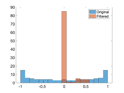
Figure 8: The spectra of the matrix, before and after applying the filter $F$ of (16)

4.2 Applying filtered matrix to a vector

Filtering the spectrum is also applicable for the case of treating the matrix as operator. Namely, when we wish to evaluate $f(A)v$ for a certain filter $f$ and vector $v$. The scenario we consider here is when a rational approximation $r(A)v\approx f(A)v$ is sufficient in terms of accuracy but evaluation time is critical. Then, we wish to further exploit the Chebyshev basis we use and the Clenshaw’s recurrence. In particular, for $r(x)=p(x)/q(x)$ we first evaluate the numerator polynomial by adapting to matrix-vector action the Clenshaw’s algorithm, see e.g., [63, Chapter 5.8]. The result is a fast algorithm for $p(A)v$. Next, we calculate $q(A)$ and solve the linear system $q(A)u=p(A)v$ to obtain $u=q(A)^{-1}p(A)v\approx r(A)v$.

In the next example, we slightly modify the filter F of (16), by setting $R=0.1$ and $r=0.1$ and discarding the identity factor. The resulted filter is a sharp bell that annihilates all components of eigenvectors which are associated with eigenvalues (roughly) outside the segment $[0.25,0.55]$. This filter, together with two of its approximations of type $(5,5)$ and type $(10,10)$, are depicted in Figure 9(a). The rational functions are calculated with an upper bound of $u=1000$ and their approximation errors, in uniform norm, are $0.0395$ and $0.0069$ for the $(5,5)$ and $(10,10)$ approximations, respectively. The matrices are of the form $A=QDQ^{\ast}\in\mathbb{R}^{k\times k}$ where the size $k$ varies from $100$ to $2500$, $Q$ is randomly selected orthogonal matrix and $D$ is a diagonal matrix with eigenvalues drawn uniformly at random over $[-1,1]$. As a benchmark, we calculate the spectral decomposition of $A$, using Matlab’s eig function, and then evaluate the filtered vector as $Q(F(D)(Q^{\ast}v))$, that is by three matrix-vector operations. The accuracy is measured in relative error $\mathinner{\!\left\lVert F(A)v-r(A)v\right\rVert}/\mathinner{\!\left\lVert v\right\rVert}$, and while the spectral decomposition presents errors of about $10^{-10}$, the rational functions obtain relative error of about $1\%$ and $5\%$, for the $(5,5)$ and $(10,10)$ approximations, respectively. Nevertheless, the benefit appears in the form of a better runtime, as presented in Figure 9(b). The runtime is measured in seconds and averaged over $10$ repeated trials. The outcome suggests that our method is faster and the gap increases as the size of the matrix grows.

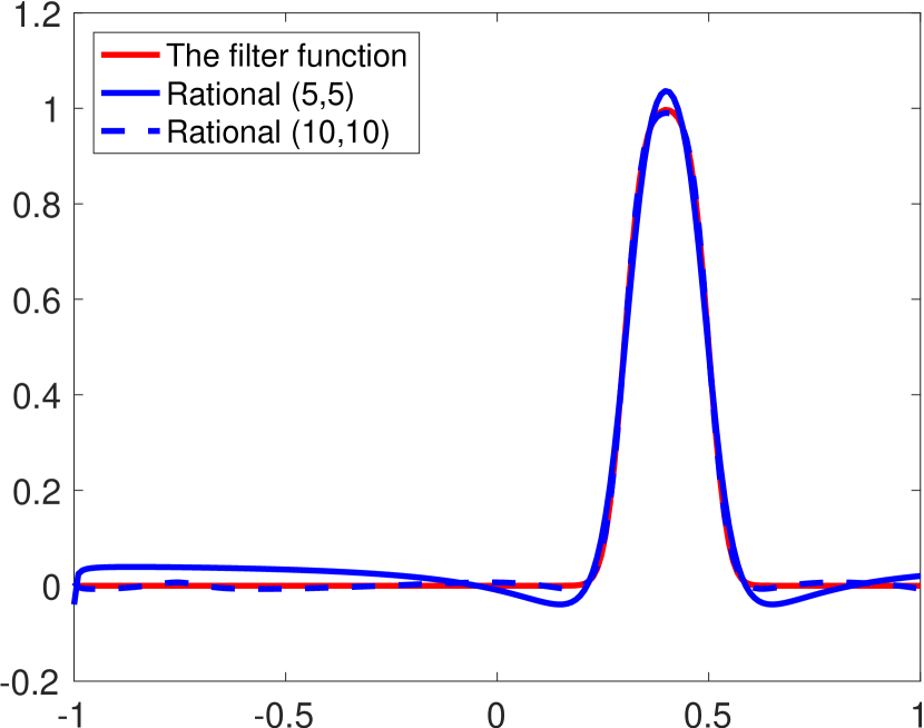
(a) The filter function and its $(5,5)$ and $(10,10)$ rational approximations

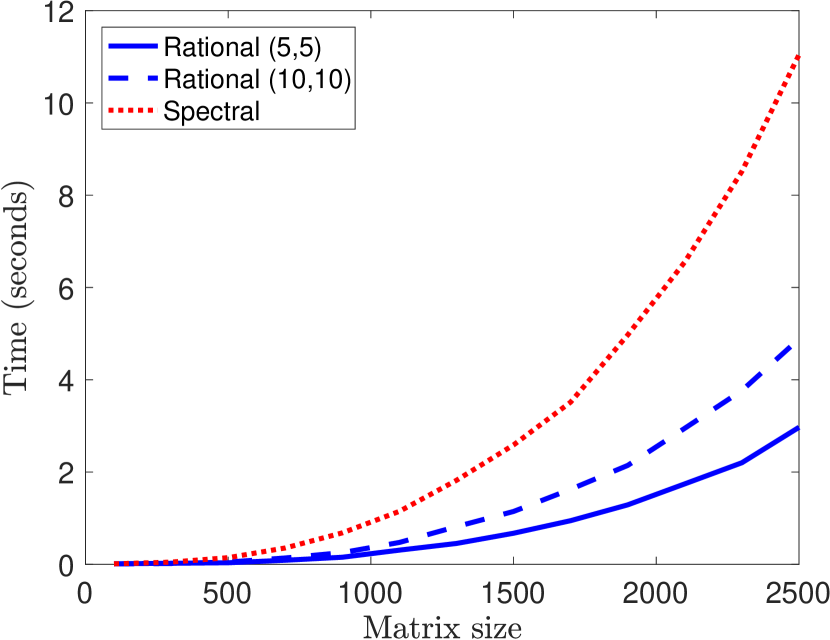
(b) The runtime

Figure 9: A runtime comparison of evaluating $f(A)v$. The results imply that evaluating the rational approximation is faster than extracting the spectral decomposition, and the difference becomes more significant as the matrix grows

4.3 From symmetric matrices to positive semidefinite matrices

While symmetric matrices have real eigenvalues, these eigenvalues are not necessarily nonnegative. The problem of projecting a symmetric matrix to the cone of semi-positive definite matrices, that is, finding the nearest positive semidefinite matrix to a symmetric matrix in the spectral norm appears in many studies, see, e.g., [13], and applications, for example, in finance industry [35] and risk management [18]. Luckily, in its plain form, this problem has a straightforward solution: calculating the spectral decomposition and then zeroing out the negative eigenvalues. This procedure solves projection with respect to the squared Frobenius norm, see e.g., [11, Chapter 8]. Nevertheless, when the matrix size increases, significant time is required to do so. Thus, different methods were proposed over time, see, e.g., [34]. Here, we provide another alternative approach; we propose to apply the function

$$f(x)=\max\{0,x\},$$ (17)

also known as ReLU (Rectified Linear Unit) function, to the symmetric matrix. The following examples illustrate this matrix function technique and compare it with the textbook solution based on the native Matlab implementation of spectral decomposition. We demonstrate the flexibility of our optimization approach, which is manifested by including positivity as a constraint. We then show that under the assumption that a moderate accuracy level is sufficient, the matrix function approach yields an efficient algorithm to solve the above problem.

As in the previous examples, we start with approximating the function, which is, in this case, $\max\{0,x\}$. One caveat of polynomial and rational approximations is that the approximant oscillates, so the required non-negativity is hard to achieve. Solutions like using Fejér kernel or damping the polynomial coefficients with suitable weights usually result in a slow convergence and lower quality approximation, see, e.g., [69]. In our method, we add a positivity constraint to the numerator, merely posing a linear constraint to the optimization problem we solve. The additional restriction reduces the search space, but the resulted accuracy turns to be comparable in magnitude. In particular, the positivity constraint slightly increases the uniform error from $0.0055$ to $0.007$ for a (5,5) type rational function with a denominator upper bound of $u=100$. The rational approximation, together with the best uniform polynomial, and the AAA rational approximation appear in Figure 10. The figure shows how our rational approximation remains positive and keeps the lowest uniform error. In addition, we show how the denominator of the AAA approximation varies across almost four orders of magnitude while our denominator keeps bounded between $1$ and $100$.

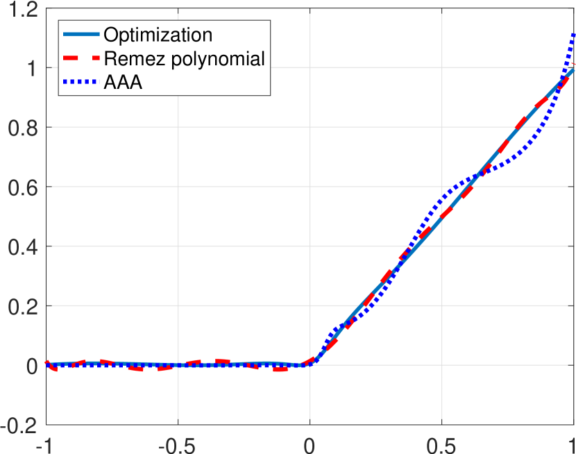
(a) The approximations to the ReLU function: two $(5,5)$ rational approximations based on our method of optimization and of AAA, and a $(10)$ degree minimax polynomial obtained by the Remez algorithm

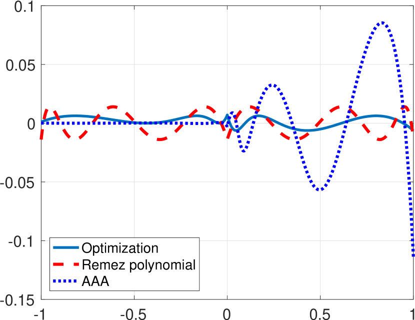
(b) The error rates. In uniform norm, the errors are $0.007$, $0.013$, and $0.114$ for the optimization, AAA, and Remez’s polynomial, respectively. Note that the AAA is much accurate on the segment $[-1,0]$ where it presents a uniform error of $0.0017$

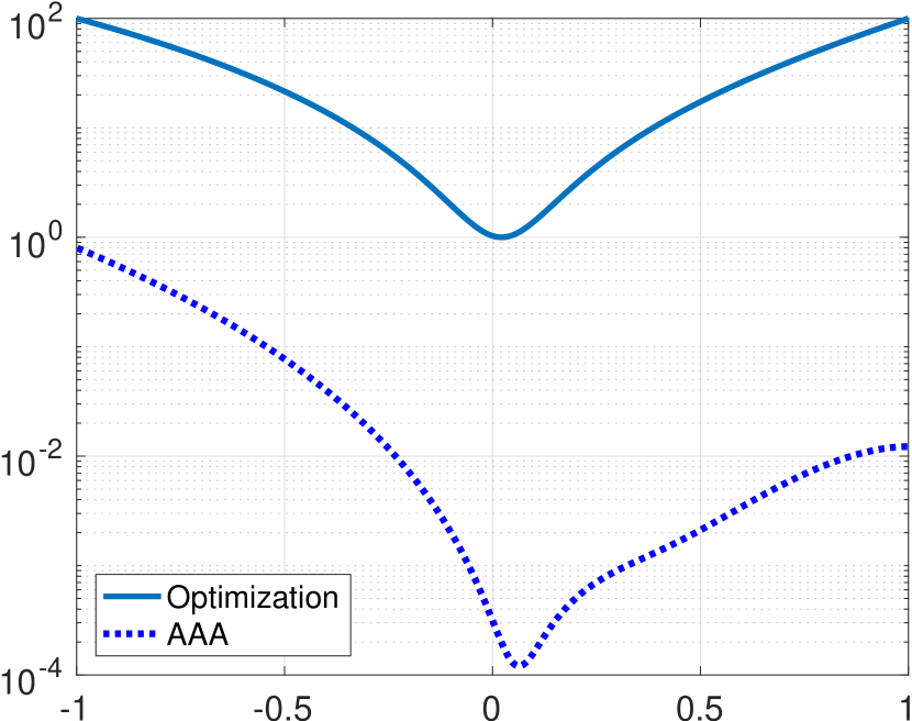
(c) The denominators of the rational approximations. Overall change value $C_{r}$ of (15) is $100$ and $6603$ for the optimization and AAA, respectively

Figure 10: Approximations of the ReLU function $\max\{0,x\}$

We propose to compute the projection of a symmetric matrix $A$ to the cone of positive semidefinite matrices as the matrix function $r(A)$ where $r(x)\approx\max\{0,x\}$. As our first test, we recall from Section 4.1 the symmetric matrix of size $100\times 100$ with Chebyshev nodes as its eigenvalues. We apply the $(5,5)$ non-negative rational approximation, as presented in Figure 10, over the matrix. Then, we plot a histogram of both the matrix and its projected version. This histogram is given in Figure 12 and shows the effect of projection as all eigenvalues are non-negative.

The second test is a time comparison, similar to Section 4.2. In particular, we compare the evaluating of $f(A)v$ where $f$ is the ReLU function of (17) and $A$ and $v$ are given matrix and a vector. The procedure is the same as in Section 4.2, so we omit it for brevity. Nevertheless, in this example, we run the test over two types of matrices. The first has eigenvalues that were uniformly drawn from $[-1,1]$. The second type of matrices has eigenvalues grouped into two narrow segments around $\pm 0.3$. Such clustered spectra are the Achilles heel of many standard spectral decomposition algorithms. Indeed, as seen in Figure 12, the runtime as a function of the matrix size increases rapidly for these matrices compares to the first kind. On the other hand, our matrix function method is blind to the different spectra, presenting similar runtime performances in both cases.

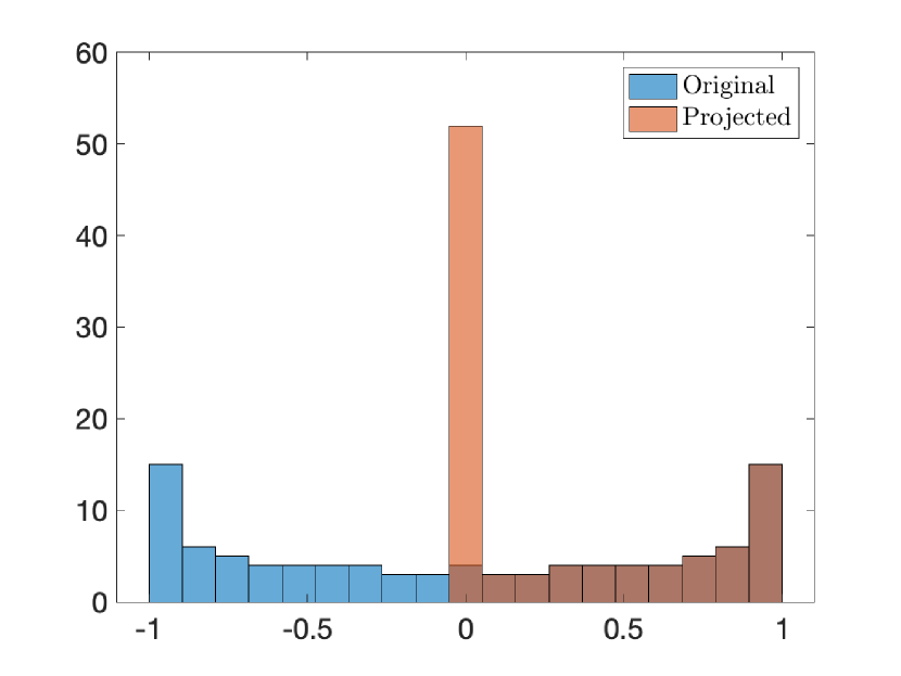
Figure 11: The spectra of the symmetric matrix before and after projection

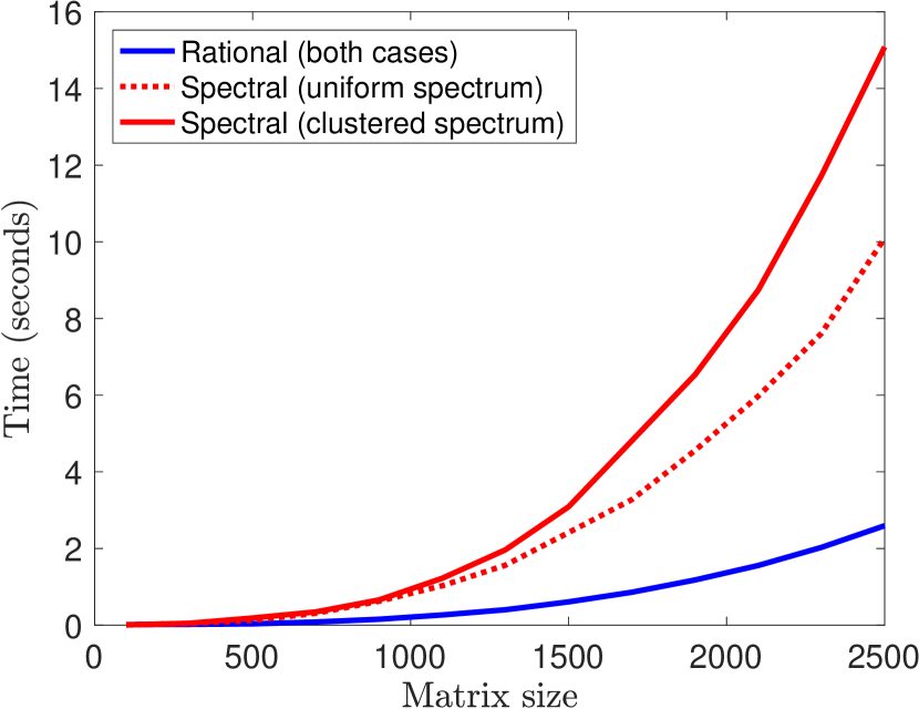
Figure 12: The time comparison of projection onto the cone of SPD matrices

5 Conclusions and future research directions

This paper demonstrates that matrix function lifting, frequently appearing in practical applications, can be tackled through rational and generalized ration approximation of the original function. This approach combines a high level of approximation accuracy and the simplicity of the computational procedures. Another essential advantage of our method is that we may naturally add more constraints to the model without destroying the efficiency. In particular, this observation is valid when the added constraints are linear. Furthermore, this extension gives rise to a number of improvements, particularly the ability to control the conditioning number of the matrices. Finally, the numerical experiments demonstrate the efficiency of our method.

Our future research directions include the possibility of having non-linear constraints as well. The first step is to extend it to the case of quasiaffine (quasilinear) additional constraints since the corresponding feasible sets remain polyhedra.

Appendix A Chebyshev polynomials

Chebyshev polynomials of the first kind of degree $n$ are defined as

$$T_{n}(x)=\cos\left(n\arccos(x)\right),\quad x\in[-1,1],\quad n=0,1,2,\ldots$$ (18)

These polynomials are solutions of the Sturm-Liouville ordinary differential equation

$$(1-x^{2})y^{\prime\prime}-xy^{\prime}+n^{2}y=0$$ (19)

and satisfy the three term recursion

$$T_{n}(x)=2xT_{n-1}(x)-T_{n-2}(x),\quad n=2,3,\ldots$$ (20)

with $T_{0}(x)=1$ and $T_{1}(x)=x$. Therefore, Chebyshev polynomials form an orthogonal basis for $L_{2}([-1,1])$ with respect to the inner product

$$\left\langle f,g\right\rangle_{T}=\frac{2}{\pi}\int_{-1}^{1}\frac{f(t)g(t)}{\sqrt{1-t^{2}}}dt.$$ (21)

The Chebyshev expansion of a function $f$ with a finite norm with respect to (21) is

$$f(x)\sim\sideset{}{{}^{\prime}}{\sum}_{n=0}^{\infty}\alpha_{n}[f]T_{n}(x),\quad\alpha_{n}[f]=\left\langle f,T_{n}\right\rangle_{T},$$ (22)

where the dashed sum $\left(\sideset{}{{}^{\prime}}{\sum}\right)$ denotes that the first term is halved. The truncated Chebyshev expansion is defined as

$$\mathcal{S}_{N}(f)(x)=\sideset{}{{}^{\prime}}{\sum}_{n=0}^{N}\alpha_{n}[f]T_{n}(x).$$ (23)

$\mathcal{S}_{N}(f)(x)$ is a polynomial approximation of $f$ which is the best least squares approximation with respect to the induced norm $\mathinner{\!\left\lVert f\right\rVert}_{T}=\sqrt{\left\langle f,f\right\rangle_{T}}$. Remarkably, this least squares approximation is close to the best minimax polynomial approximation, and in particular the following was established by Bernstein [9]

$$\mathinner{\!\left\lVert f(x)-S_{N}(f)(x)\right\rVert}_{\infty}\leq\Lambda_{N}\mathinner{\!\left\lVert f(x)-p^{\ast}_{N}(x)\right\rVert}_{\infty},\quad f\in C([-1,1]),$$

where $p^{\ast}_{N}$ is the unique best minimax polynomial approximation of degree $N$, and Lebesgue constant $\Lambda_{N}$ behaves asymptotically as $\log(N)$ for large $N$. For the exact value see [62] (and in particular, it is less than $6$ for $N<1000$).

The Chebyshev polynomials satisfy a discrete orthogonality relation as well as the continuous one (with respect to (21)). Specifically, denote by $z_{n}$, $n=1,\ldots,N$ the zeros of $T_{N}$. Then, for any $0\leq\ell\neq k<N$ we have

$$\sum_{n=1}^{N}T_{\ell}(z_{n})T_{k}(z_{n})=0.$$ (24)

The above is essential in calculating $\alpha_{n}$ of (23) and plays a significant role in stabilizing our optimization that uses the representation (6). For more information, we refer the interested reader to [63, Chapter 5].

References

- [1] Mohamed Abdalla. Special matrix functions: characteristics, achievements and future directions. Linear and Multilinear Algebra, 68(1):1–28, 2020.
- [2] Athanasios C Antoulas and Brian DO Anderson. On the scalar rational interpolation problem. IMA Journal of Mathematical Control and Information, 3(2-3):61–88, 1986.
- [3] Francesca Arrigo, Michele Benzi, and Caterina Fenu. Computation of generalized matrix functions. SIAM Journal on Matrix Analysis and Applications, 37(3):836–860, 2016.
- [4] Haim Avron, Michael Kapralov, Cameron Musco, Christopher Musco, Ameya Velingker, and Amir Zandieh. A universal sampling method for reconstructing signals with simple fourier transforms. In Proceedings of the 51st Annual ACM SIGACT Symposium on Theory of Computing, pages 1051–1063, 2019.
- [5] Ian Barrodale, Michael JD Powell, and Frank DK Roberts. The differential correction algorithm for rational approximation. SIAM Journal on Numerical Analysis, 9(3):493–504, 1972.
- [6] Heinz H Bauschke and Adrian S Lewis. Dykstras algorithm with Bregman projections: A convergence proof. Optimization, 48(4):409–427, 2000.
- [7] Bernhard Beckermann, George Labahn, and Ana C Matos. On rational functions without froissart doublets. Numerische Mathematik, 138(3):615–633, 2018.
- [8] Peter Benner, Steffen Börm, Thomas Mach, and Knut Reimer. Computing the eigenvalues of symmetric -matrices by slicing the spectrum. Computing and Visualization in Science, 16(6):271–282, 2013.
- [9] Serge Bernstein. Quelques remarques sur l’interpolation. Mathematische Annalen, 79(1):1–12, 1918.
- [10] Jean-Philippe Bouchaud and Marc Potters. Financial applications of random matrix theory: a short review, 2009.
- [11] Stephen Boyd, Stephen P Boyd, and Lieven Vandenberghe. Convex optimization. Cambridge university press, 2004.
- [12] Stephen Boyd and Lieven Vandenberghe. Convex Optimization. Cambridge University Press, New York, NY, USA, 2010.
- [13] Stephen Boyd and Lin Xiao. Least-squares covariance matrix adjustment. SIAM Journal on Matrix Analysis and Applications, 27(2):532–546, 2005.
- [14] Dietrich Braess. Nonlinear approximation theory, volume 7. Springer Science & Business Media, New York, NY, USA, 2012.
- [15] Claude Brezinski and Michela Redivo-Zaglia. Padé–type rational and barycentric interpolation. Numerische Mathematik, 125(1):89–113, 2013.
- [16] Buck R. Creighton. Applications of duality in approximation theory. In: Approximation of Functions. Elsevier, Amsterdam, Netherlands, 1965.
- [17] Jean Pierre Crouzeix. Conditions for convexity of quasiconvex functions. Mathematics of Operations Research, 5(1):120–125, 1980.
- [18] Stefan Cutajar, Helena Smigoc, and Adrian O’Hagan. Actuarial risk matrices: The nearest positive semidefinite matrix problem. North American Actuarial Journal, 21(4):552–564, 2017.
- [19] Aris Daniilidis, Nicolas Hadjisavvas, and Juan-Enrique Martinez-Legaz. An appropriate subdifferential for quasiconvex functions. SIAM Journal on Optimization, 12:407–420, 2002.
- [20] Bruno De Finetti. Sulle stratificazioni convesse. Annali di Matematica Pura ed Applicata, 30(1):173–183, 1949.
- [21] Emilio Defez, Javier Ibáñez, Jesús Peinado, Jorge Sastre, and Pedro Alonso-Jordá. An efficient and accurate algorithm for computing the matrix cosine based on new hermite approximations. Journal of Computational and Applied Mathematics, 348:1–13, 2019.
- [22] Emilio Defez, Jorge Sastre, Javier Ibanez, and Jesus Peinado. Solving engineering models using hyperbolic matrix functions. Applied Mathematical Modelling, 40(4):2837–2844, 2016.
- [23] Vladimir F Demyanov, Panos M Pardalos, and Mikhail Batsyn. Constructive Nonsmooth Analysis and Related Topics. Springer, New York, NY, USA, 2014.
- [24] Frank R Deutsch. Simultaneous interpolation and approximation in topological linear spaces. SIAM Journal on Applied Mathematics, 14:1180–1190, 1966.
- [25] Vladimir Druskin, Alexander V Mamonov, and Mikhail Zaslavsky. Multiscale s-fraction reduced-order models for massive wavefield simulations. Multiscale Modeling & Simulation, 15(1):445–475, 2017.
- [26] Massimiliano Fasi and Nicholas J Higham. Multiprecision algorithms for computing the matrix logarithm. SIAM Journal on Matrix Analysis and Applications, 39(1):472–491, 2018.
- [27] Massimiliano Fasi and Nicholas J Higham. An arbitrary precision scaling and squaring algorithm for the matrix exponential. SIAM Journal on Matrix Analysis and Applications, 40(4):1233–1256, 2019.
- [28] Silviu-Ioan Filip, Yuji Nakatsukasa, Lloyd N Trefethen, and Bernhard Beckermann. Rational minimax approximation via adaptive barycentric representations. SIAM Journal on Scientific Computing, 40(4):A2427–A2455, 2018.
- [29] Andreas Frommer and Valeria Simoncini. Matrix functions. In Model order reduction: theory, research aspects and applications, pages 275–303. Springer, New York, NY, USA, 2008.
- [30] Evan S Gawlik. Zolotarev iterations for the matrix square root. SIAM journal on matrix analysis and applications, 40(2):696–719, 2019.
- [31] Karl Glashoff and Sven-Åke Gustafson. Linear Optimization and Approximation, volume 45. Springer, New York, NY, USA, 1983.
- [32] Miguel A Goberna and Marco A López. A comprehensive survey of linear semi-infinite optimization theory. In Semi-infinite programming, pages 3–27. Springer, New York, NY, USA, 1998.
- [33] Pedro Gonnet, Stefan Guttel, and Lloyd N Trefethen. Robust padé approximation via svd. SIAM review, 55(1):101–117, 2013.
- [34] Nicholas J Higham. Accuracy and stability of numerical algorithms. SIAM, Philadelphia, USA, 2002.
- [35] Nicholas J Higham. Computing the nearest correlation matrix—a problem from finance. IMA journal of Numerical Analysis, 22(3):329–343, 2002.
- [36] Nicholas J Higham. Functions of matrices: theory and computation, volume 104. SIAM, Philadelphia, PA, USA, 2008.
- [37] Nicholas J Higham and Peter Kandolf. Computing the action of trigonometric and hyperbolic matrix functions. SIAM Journal on Scientific Computing, 39(2):A613–A627, 2017.
- [38] Jeffrey M Hokanson and Caleb C Magruder. Least squares rational approximation, 2018.
- [39] Richard B Holmes. A Course on Optimization and Best Approximation. Springer-Verlag, New York, NY, USA, 1972.
- [40] Richard B Holmes. -splines in Banach spaces. I. Interpolation of linear manifolds. Journal of Mathematical Analysis and Applications, 40:574–593, 1972.
- [41] Narendra Karmarkar. A new polynomial-time algorithm for linear programming. In Proceedings of the sixteenth annual ACM symposium on Theory of computing, pages 302–311, 1984.
- [42] Charles S Kenney and Alan J Laub. The matrix sign function. IEEE transactions on automatic control, 40(8):1330–1348, 1995.
- [43] Pierre Jean Laurent. Approximation et optimisation. Hermann, Paris, France, 1972.
- [44] Olivier Ledoit and Michael Wolf. Analytical nonlinear shrinkage of large-dimensional covariance matrices. Annals of Statistics, 48(5):3043–3065, 2020.
- [45] Ron Levie, Federico Monti, Xavier Bresson, and Michael M Bronstein. Cayleynets: Graph convolutional neural networks with complex rational spectral filters. IEEE Transactions on Signal Processing, 67(1):97–109, 2018.
- [46] Mengmeng Li and JinRong Wang. Exploring delayed mittag-leffler type matrix functions to study finite time stability of fractional delay differential equations. Applied Mathematics and Computation, 324:254–265, 2018.
- [47] Ruipeng Li, Yuanzhe Xi, Lucas Erlandson, and Yousef Saad. The eigenvalues slicing library (evsl): Algorithms, implementation, and software. SIAM Journal on Scientific Computing, 41(4):C393–C415, 2019.
- [48] Henry L Loeb. Algorithms for Chebyshev approximations using the ratio of linear forms. Journal of the Society for Industrial and Applied Mathematics, 8(3):458–465, 1960.
- [49] Juan E Martínez-Legaz. Quasiconvex duality theory by generalized conjugation methods. Optimization, 19(5):603–652, 1988.
- [50] Victor May, Yossi Keller, Nir Sharon, and Yoel Shkolnisky. An algorithm for improving non-local means operators via low-rank approximation. IEEE Transactions on Image Processing, 25(3):1340–1353, 2016.
- [51] Robert Mayans. The Chebyshev equioscillation theorem, 2006.
- [52] Günter Meinardus. Approximation of functions: Theory and numerical methods, volume 13. Springer Science & Business Media, New York, NY, USA, 2012.
- [53] Prashanth Nadukandi and Nicholas J Higham. Computing the wave-kernel matrix functions. SIAM Journal on Scientific Computing, 40(6):A4060–A4082, 2018.
- [54] Yuji Nakatsukasa and Roland W Freund. Computing fundamental matrix decompositions accurately via the matrix sign function in two iterations: The power of zolotarev’s functions. SIAM Review, 58(3):461–493, 2016.
- [55] Yuji Nakatsukasa, Olivier Sète, and Lloyd N Trefethen. The AAA algorithm for rational approximation. SIAM Journal on Scientific Computing, 40(3):A1494–A1522, 2018.
- [56] JX Da Cruz Neto, JO Lopes, and MV Travaglia. Algorithms for quasiconvex minimization. Optimization, 60(8-9):1105–1117, 2011.
- [57] D J Newman. Rational approximation to . The Michigan Mathematical Journal, 11(1):11–14, 1964.
- [58] V Noferini. A formula for the fréchet derivative of a generalized matrix function. SIAM Journal on Matrix Analysis and Applications, 38(2):434–457, 2017.
- [59] Ricardo Pachón and Lloyd N Trefethen. Barycentric-remez algorithms for best polynomial approximation in the chebfun system. BIT Numerical Mathematics, 49(4):721, 2009.
- [60] Vinesha Peiris, Nir Sharon, Nadezda Sukhorukova, and Julien Ugon. Generalised rational approximation and its application to improve deep learning classifiers. Applied Mathematics and Computation, 389:125560, 2021.
- [61] Vinesha Peiris and Nadezda Sukhorukova. The extension of the linear inequality method for generalized rational chebyshev approximation to approximation by general quasilinear functions. Optimization, 71(4):999–1019, 2022.
- [62] Michael J D Powell. On the maximum errors of polynomial approximations defined by interpolation and by least squares criteria. The Computer Journal, 9(4):404–407, 1967.
- [63] William H Press, H William, Saul A Teukolsky, William T Vetterling, A Saul, and Brian P Flannery. Numerical recipes 3rd edition: The art of scientific computing. Cambridge university press, New York, NY, USA, 2007.
- [64] Anthony Ralston. Rational Chebyshev approximation by Remes’ algorithms. Numerische Mathematik, 7(4):322–330, 1965.
- [65] Eugene Y Remez. Sur le calcul effectif des polynomes d’approximation de tchebichef. Comptes Rendus de l’Académie des Sciences de Paris, 199:337–340, 1934.
- [66] Alexander M. Rubinov. Abstract Convexity and Global Optimization. Kluwer Academic Publishers, New York, NY, USA, 2000.
- [67] Alexander M Rubinov and Joydeep Dutta. Abstract convexity. In Handbook of generalized convexity and generalized monotonicity, pages 293–333. Springer, Boston, MA, USA, 2005.
- [68] Alexander M Rubinov and B Simsek. Conjugate quasiconvex nonnegative functions. Optimization, 35(1):1–22, 1995.
- [69] Yousef Saad. Numerical methods for large eigenvalue problems: revised edition. SIAM, Philadelphia, USA, 2011.
- [70] Nir Sharon and Yoel Shkolnisky. Evaluating non-analytic functions of matrices. Journal of Mathematical Analysis and Applications, 462(1):613–636, 2018.
- [71] Herbert Stahl. Uniform rational approximation of| x|. In Methods of approximation theory in complex analysis and mathematical physics, pages 110–130. Springer, 1993.
- [72] Vadim Stotland, Oded Schwartz, and Sivan Toledo. High-performance direct algorithms for computing the sign function of triangular matrices. Numerical Linear Algebra with Applications, 25(2):e2139, 2018.
- [73] Nadezda Sukhorukova and Julien Ugon. Characterization theorem for best polynomial spline approximation with free knots. Transactions of the American Mathematical Society, 369:6389–6405, 2017.
- [74] Lloyd N Trefethen. Approximation Theory and Approximation Practice, Extended Edition. SIAM, Philadelphia, PA, USA, 2019.
- [75] Marc Van Barel and Adhemar Bultheel. A parallel algorithm for discrete least squares rational approximation. Numerische Mathematik, 63(1):99–121, 1992.
- [76] Marcus Webb, Lloyd N Trefethen, and Pedro Gonnet. Stability of barycentric interpolation formulas for extrapolation. SIAM Journal on Scientific Computing, 34(6):A3009–A3015, 2012.
- [77] Yuanzhe Xi and Yousef Saad. Computing partial spectra with least-squares rational filters. SIAM Journal on Scientific Computing, 38(5):A3020–A3045, 2016.
- [78] Shin ya Matsushita and Li Xu. On the finite termination of the Douglas-Rachford method for the convex feasibility problem. Optimization, 65(11):2037–2047, 2016.
- [79] Yuning Yang and Qingzhi Yang. Some modified relaxed alternating projection methods for solving the two-sets convex feasibility problem. Optimization, 62(4):509–525, 2013.
- [80] A. J. Zaslavski. Subgradient projection algorithms and approximate solutions of convex feasibility problems. Journal of Optimization Theory and Applications, 157:803–819, 2013.
- [81] Ahmed I Zayed. Advances in Shannon’s sampling theory. Routledge & CRC, Boca Raton, FL, USA, 2018.
- [82] Xiaopeng Zhao and Markus Arthur Köbis. On the convergence of general projection methods for solving convex feasibility problems with applications to the inverse problem of image recovery. Optimization, 67(9):1409–1427, 2018.