Higgs boson decay to the pair of S- and P-wave $B_{c}$ mesons

Abstract

We investigate the rare production of the pair of S- and P-wave $B_{c}$-meson in the Higgs boson decay in the perturbative Standard Model and relativistic quark model. Relativistic amplitudes and decay widths are constructed with the account of the relative motion of heavy quarks forming $B_{c}$ mesons. When constructing the Higgs boson decay amplitudes, the method of projection operators on the S- and P-wave states of quarks is used. Relativistic corrections are expressed in terms of special relativistic parameters and are calculated numerically in the quark model. The dependence of the decay widths of the Higgs boson on various sources of relativistic corrections is investigated.

I Introduction

The study of properties of the Higgs boson and its decays began immediately after its discovery by the ATLAS and CMS experiments at the LHC [1, 2]. At present, a detailed study of the Higgs sector is the important direction in particle physics. The large mass of the Higgs boson, as well as significant coupling constants with gauge bosons and quarks, provide a variety of decay channels [3, 4, 5, 6, 7, 8, 9]. The analysis of various decays is based on a set of proton-proton collision data collected with detectors at the CERN Large Hadron Collider. Main decay channels of the Higgs boson are connected with the production of photons, W, Z bosons and heavy quarks. Investigation of various mechanisms of heavy quarkonia production in Higgs boson decays is of obvious interest in connection with testing various approaches to describing the production of heavy quarks and their bound states. Among the decay processes of the Higgs boson, one can single out a rare exclusive process in which a pair of $B_{c}$ mesons is formed in different S- and P-states. For a reliable description of the amplitudes of such processes, it is important to have a consistent theory of the production of a pair of bound states of quarks and antiquarks, in which the effects of the relative motion of heavy quarks are strictly taken into account. Such processes are also interesting in the sense that a pair of $B_{c}$ mesons is produced here, which, in contrast to charmonium and bottomonium, have been studied to a much lesser extent experimentally. Bound states of two different heavy quarks $(\bar{b}c)$ with open beauty and charm stand out in a significant way among heavy quarkonia since its decay mechanism differs significantly from the decay mechanism of charmonium or bottomonium. There is a hope that the processes of pair production of $B_{c}$ mesons in various states can be investigated experimentally from the decay products of $B_{c}$ mesons. In this work, we continue the study of relativistic effects during the production of a pair of $B_{c}$ mesons in Higgs boson decays [10], including in the field of study not only S-wave, but also P-wave $B_{c}$ mesons. We study the relativistic corrections both in the production amplitude of two quarks and antiquarks, and in the transformation law of the wave functions of $B_{c}$ mesons during the transition from the rest frame to the moving reference frame. As known from our previous studies the corrections of these types significantly contribute to the production cross section of a pair of heavy quarkonia [11, 12, 13].

Our approach to the study of Higgs boson decays includes a perturbative stage, when two free quarks and two antiquarks are created, and a nonperturbative stage, in which the formation of quarks bound states occurs. The nonperturbative part of the meson production process is described within the framework of the relativistic quark model. This mechanism of production of a pair of $B_{c}$ mesons, which we call quark, is further considered in detail in the following sections. Within this approach, we can systematically take into account relativistic effects at all stages of the decay process, including the formation of $B_{c}$ mesons due to the strong interaction of quarks. Taking into account relativistic effects in the production of heavy quarkonia in various reactions is very important for achieving good accuracy in calculating the observed quantities [14].

One of the first works devoted to the pair production of quarkonia in Higgs boson decays was done in the nonrelativistic approximation in [3]. The production of single quarkonia in the H decay was investigated in [4, 5] with the account of relativistic corrections and one-loop corrections. In the work [6], various channels of the Higgs boson decay into pairs of heavy quarkonia were studied, including $H\to ZZ$, $H\to WW$. Single $B_{c}$ meson and double heavy baryon production rates in Higgs boson decays were calculated in the nonrelativistic QCD framework in [7, 8]. The observations of the Higgs boson decays into a pair $\gamma\gamma$, $WW$, $ZZ$, $b\bar{b}$ and $\tau\tau$ have been reported in [15, 16, 17, 18]. The first experimental searches for decays of the Higgs boson into a pair of $J/\Psi$ and $\Upsilon$ mesons were performed in [19]. If the bound states of the same heavy quarks and antiquarks have been studied experimentally well enough, the bound states of different heavy quarks were observed much less frequently [20]. In fact, $B_{c}$ mesons are known only for the $1S$ and $2S$ states. Therefore, the study of various mechanisms for the production of S-wave and P-wave $B_{c}$ mesons is of obvious interest, which is connected with the study of their properties.

II General formalism

Four quark production amplitudes of the $B_{c}$ meson pair in leading order of the QCD coupling constant $\alpha_{s}$ are presented in Fig. 1. We investigate the production channel of a pair of $B_{c}$ mesons connected with the initial production of a pair of heavy quarks $b$ or $c$ in the Higgs boson decay. There are two stages of $B_{c}$ meson production process. At the first stage, which is described by the perturbative Standard Model, the Higgs boson transforms into a heavy quark-antiquark pair. Then the heavy quark or antiquark emits a virtual gluon which produces another heavy quark-antiquark pair. At the second stage, heavy quarks and antiquarks combine with some probability into bound states.

Four-momenta of heavy quarks and antiquarks can be expressed in terms of relative and total four momenta as follows:

$$p_{1}=\eta_{1}P+p,~{}p_{2}=\eta_{2}P-p,~{}(p\cdot P)=0,~{}\eta_{i}=\frac{M_{1}^{2}\pm m_{1}^{2}\mp m_{2}^{2}}{2M_{1}^{2}},$$ (1)

$$q_{1}=\rho_{1}Q+q,~{}q_{2}=\rho_{2}Q-q,~{}(q\cdot Q)=0,~{}\rho_{i}=\frac{M_{2}^{2}\pm m_{1}^{2}\mp m_{2}^{2}}{2M_{2}^{2}},$$

where $M_{1}$ and $M_{2}$ are the masses of $B_{c}^{+}$ and $B_{c}^{-}$ mesons consisting of $\bar{b}c$ and $\bar{c}b$. $m_{1,2}$ are the masses of $c$ and $b$ quarks. Neglecting the effects of particle coupling, we obtain $\rho_{1}\approx\eta_{1}\approx m_{1}/(m_{1}+m_{2})$, $\rho_{2}\approx\eta_{2}\approx m_{2}/(m_{1}+m_{2})$. $P$, $Q$ are the total four-momenta of mesons $B_{c}^{+}$ and $B_{c}^{-}$, relative quark four-momenta $p=L_{P}(0,{\bf p})$ and $q=L_{P}(0,{\bf q})$ are obtained from the rest frame four-momenta $(0,{\bf p})$ and $(0,{\bf q})$ by the Lorentz transformation to the system moving with the momenta $P$ and $Q$. The index $i=1,2$ corresponds to plus and minus signs in (1). Heavy quarks $c$, $b$ and antiquarks $\bar{c}$, $\bar{b}$ are outside the mass shell in the intermediate state: $p_{1,2}^{2}=\eta_{1,2}^{2}P^{2}-{\bf p}^{2}=\eta_{1,2}^{2}M_{1}^{2}-{\bf p}^{2}\not=m_{1,2}^{2}$, so that $p_{1}^{2}-m_{1}^{2}=p_{2}^{2}-m_{2}^{2}$.

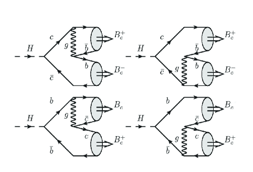
Figure 1: The quark mechanism for the production of a pair of $B_{c}$ mesons in the decay of the Higgs boson. Dashed line shows the Higgs boson and wavy line corresponds to the gluon.

In this work we study the production of S-wave and P-wave $B_{c}$ mesons. It is convenient to begin the construction of the pair production amplitudes with a description of the production of S-wave $B_{c}$ states. Let consider the production amplitude of two pseudoscalar and two vector $B_{c}$ mesons setting $M_{1}=M_{2}=M_{B_{c}}$. Initially it can be written as a convolution of perturbative production amplitude of free quarks and antiquarks and the quasipotential wave functions of $B_{c}$ mesons moving with four-momenta P and Q. Using then the transformation law of the bound state wave functions from the rest frame to the moving one with four-momenta $P$ and $Q$ we can present the meson production amplitude in the form [11, 12, 21]:

$${\cal M}(P,Q)=-i(\sqrt{2}G_{F})^{\frac{1}{2}}\frac{2\pi}{3}M_{B_{c}}\int\frac{d{\bf p}}{(2\pi)^{3}}\int\frac{d{\bf q}}{(2\pi)^{3}}\times$$ (2)

$$\times Tr\left\{\Psi^{\cal P,V}_{B_{c}}(p,P)\Gamma_{1}^{\nu}(p,q,P,Q)\Psi^{\cal P,V}_{B_{c}}(q,Q)\gamma_{\nu}+\Psi^{\cal P,V}_{B_{c}}(q,Q)\Gamma_{2}^{\nu}(p,q,P,Q)\Psi^{\cal P,V}_{B_{c}}(p,P)\gamma_{\nu}\right\},$$

where a superscript ${\cal P}$ indicates a pseudoscalar $B_{c}$ meson, a superscript ${\cal V}$ indicates a vector $B_{c}$ meson, $G_{F}$ is the Fermi constant. $\Gamma_{1,2}$ are the vertex functions defined below. The permutation of subscripts $b$ and $c$ in the wave functions indicates corresponding permutation in the projection operators (see below Eqs.(4)-(6)). The method for producing the amplitudes in the form (2) is described in detail in our previous studies [21, 13, 22]. The transition of free quark-antiquark pair to meson bound states is described in our approach by specific wave functions. Relativistic wave functions of pseudoscalar and vector $B_{c}$ mesons accounting for the transformation from the rest frame to the moving one with four momenta $P$, and $Q$ are

$$\Psi^{\cal P}_{B_{c}}(p,P) = \frac{\Psi^{0}_{B_{c}}({\bf p})}{\sqrt{\frac{\epsilon_{1}(p)}{m_{1}}\frac{(\epsilon_{1}(p)+m_{1})}{2m_{1}}\frac{\epsilon_{2}(p)}{m_{2}}\frac{(\epsilon_{2}(p)+m_{2})}{2m_{2}}}}\left[\frac{\hat{v}_{1}-1}{2}+\hat{v}_{1}\frac{{\bf p}^{2}}{2m_{2}(\epsilon_{2}(p)+m_{2})}-\frac{\hat{p}}{2m_{2}}\right]$$ (4)

$$\times\gamma_{5}(1+\hat{v}_{1})\left[\frac{\hat{v}_{1}+1}{2}+\hat{v}_{1}\frac{{\bf p}^{2}}{2m_{1}(\epsilon_{1}(p)+m_{1})}+\frac{\hat{p}}{2m_{1}}\right],$$

$$\Psi^{\cal V}_{B^{\ast}_{c}}(q,Q) = \frac{\Psi^{0}_{B^{\ast}_{c}}({\bf q})}{\sqrt{\frac{\epsilon_{1}(q)}{m_{1}}\frac{(\epsilon_{1}(q)+m_{1})}{2m_{1}}\frac{\epsilon_{2}(q)}{m_{2}}\frac{(\epsilon_{2}(q)+m_{2})}{2m_{2}}}}\left[\frac{\hat{v}_{2}-1}{2}+\hat{v}_{2}\frac{{\bf q}^{2}}{2m_{1}(\epsilon_{1}(q)+m_{1})}+\frac{\hat{q}}{2m_{1}}\right]$$ (6)

$$\times\hat{\varepsilon}(Q,S_{z})(1+\hat{v}_{2})\left[\frac{\hat{v}_{2}+1}{2}+\hat{v}_{2}\frac{{\bf q}^{2}}{2m_{2}(\epsilon_{2}(q)+m_{2})}-\frac{\hat{q}}{2m_{2}}\right],$$

where the symbol hat denotes convolution of four-vector with the Dirac gamma matrices, $v_{1}=P/M_{B_{c}}$, $v_{2}=Q/M_{B_{c}}$; $\varepsilon^{\lambda}(Q,S_{z})$ is the polarization vector of the $B^{\ast-}_{c}(1^{-})$ meson, relativistic quark energies $\epsilon_{1,2}(p)=\sqrt{p^{2}+m_{1,2}^{2}}$. In (4) and (6) we have complicated factor depending on relative momenta ${\bf p}$, ${\bf q}$ including the bound state wave function in the rest frame $\Psi^{0}_{B_{c}}({\bf p})$. The production amplitude (2) contains the integration over the quark relative momenta ${\bf p}$ and ${\bf q}$. The result of integration essentially depends on the wave functions of bound states of heavy quarks. The color part of the meson wave function in the amplitude (2) is taken as $\delta_{ij}/\sqrt{3}$ (color indexes $i,j,k=1,2,3$). Relativistic wave functions in (4) and (6) are equal to the product of wave functions in the rest frame $\Psi^{0}_{B_{c}}({\bf p})$ and spin projection operators that are accurate at all orders in $|{\bf p}|/m$ and $|{\bf q}|/m$. An expression of spin projector in different form for $(c\bar{c})$ system was obtained in [23] where spin projectors are written in terms of heavy quark momenta $p_{1,2}$ lying on the mass shell. Our derivation of relations (4) and (6) accounts for the transformation law of the bound state wave functions from the rest frame to the moving one with four momenta $P$ and $Q$. This transformation law was discussed in the Bethe-Salpeter approach in [24] and in quasipotential method in [25].

II.1 Production of a pair of $B_{c}$ mesons in S-states

When constructing the decay amplitudes with the production of a pair of S-wave $B_{c}$ mesons, we introduce projection operators $\hat{\Pi}^{\cal P,V}$ for states with total spin $S=0,~{}1$ of the following form:

$$\hat{\Pi}^{\cal P}=[v_{2}(0)\bar{u}_{1}(0)]_{S=0}=\gamma_{5}\frac{1+\gamma^{0}}{2\sqrt{2}},~{}~{}~{}\hat{\Pi}^{\cal V}=[v_{2}(0)\bar{u}_{1}(0)]_{S=1}=\hat{\varepsilon}\frac{1+\gamma^{0}}{2\sqrt{2}}.$$ (7)

After that, the total amplitude of the Higgs boson decay in the leading order in strong coupling constant $\alpha_{s}$ can be represented in the form:

$${\mathcal{M}}=\frac{4\pi}{3}M_{B_{c}}\int\!\frac{d\mathbf{p}}{(2\pi)^{3}}\int\!\frac{d\mathbf{q}}{(2\pi)^{3}}\mathrm{Tr}\bigl{\{}\mathcal{T}_{12}+\mathcal{T}_{34}\bigr{\}},$$ (8)

$${\mathcal{T}_{12}}=\Gamma_{c}\alpha_{b}\Psi^{\cal P,V}_{B_{c}}(p,P)\left[\frac{\hat{p}_{1}-\hat{r}+m_{1}}{(r-p_{1})^{2}-m_{1}^{2}}\,\gamma_{\mu}+\gamma_{\mu}\,\frac{\hat{r}-\hat{q}_{1}+m_{1}}{(r-q_{1})^{2}-m_{1}^{2}}\right]D^{\mu\nu}(k_{2})\Psi^{\cal P,V}_{B_{c}}(q,Q)\gamma_{\nu},$$ (9)

$${\mathcal{T}_{34}}=\Gamma_{b}\alpha_{c}\Psi^{\cal P,V}_{B_{c}}(q,Q)\left[\frac{\hat{p}_{2}-\hat{r}+m_{2}}{(r-p_{2})^{2}-m_{2}^{2}}\,\gamma_{\mu}+\gamma_{\mu}\frac{\hat{r}-\hat{q}_{2}+m_{2}}{(r-q_{2})^{2}-m_{2}^{2}}\,\right]D^{\mu\nu}(k_{1})\Psi^{\cal P,V}_{B_{c}}(p,P)\gamma_{\nu},$$ (10)

where subscripts 12, 34 denote the contributions of amplitudes 1 and 2, 3 and 4 in Fig. 1, $\alpha_{c,b}=\alpha_{s}\left(m_{1,2}^{2}M_{H}^{2}/(m_{1}+m_{2})^{2}\Lambda^{2}\right)$. $\Gamma_{c}=m_{1}(\sqrt{2}G_{F})^{\frac{1}{2}}$, $\Gamma_{b}=m_{2}(\sqrt{2}G_{F})^{\frac{1}{2}}$. The trace calculation in (8) leads to amplitudes ${\cal M}_{PP}$ and ${\cal M}_{VV}$ presented in (14)-(15). Four-momentum of Higgs boson squared $r^{2}=M_{H}^{2}=(P+Q)^{2}=2M_{B_{c}}^{2}+2PQ$, the gluon four-momenta are $k_{1}=p_{1}+q_{1}$, $k_{2}=p_{2}+q_{2}$. Relative momenta $p$, $q$ of heavy quarks enter in the gluon propagators $D_{\mu\nu}(k_{1,2})$ and quark propagators as well as in relativistic wave functions (4) and (6). Accounting for the small ratio of relative quark momenta $p$ and $q$ to the mass of the Higgs boson $M_{H}$, we can simplify the inverse denominators of quark and gluon propagators as follows:

$$\frac{1}{(p_{1}+q_{1})^{2}}=\frac{1}{\eta_{1}^{2}M_{H}^{2}},~{}~{}~{}\frac{1}{(p_{2}+q_{2})^{2}}=\frac{1}{\eta_{2}^{2}M_{H}^{2}},$$ (11)

$$\frac{1}{(r-q_{1})^{2}-m_{1}^{2}}=\frac{1}{\eta_{2}M_{H}^{2}},~{}~{}~{}\frac{1}{(-r-p_{1})^{2}-m_{1}^{2}}=\frac{1}{\eta_{2}M_{H}^{2}},$$ (12)

$$\frac{1}{(r-p_{2})^{2}-m_{1}^{2}}=\frac{1}{\eta_{1}M_{H}^{2}},~{}~{}~{}\frac{1}{(-r-q_{2})^{2}-m_{1}^{2}}=\frac{1}{\eta_{1}M_{H}^{2}}.$$ (13)

In the case of $B_{c}$ meson production of the same mass $\rho_{1}=\eta_{1}$, $\rho_{2}=\eta_{2}$. The formulas (11)-(13) mean that we completely neglect corrections of the form $|{\bf p}|/M_{H}$, $|{\bf q}|/M_{H}$. At the same time, we keep in the amplitudes (9), (10) the second-order correction for small ratios $|{\bf p}|/m_{1,2}$, $|{\bf q}|/m_{1,2}$ relative to the leading order result. As we take relativistic factors in the denominator of the amplitudes (4) and (6) unchanged, the momentum integrals are convergent. Calculating the trace in obtained expression in the package FORM [26], we find relativistic amplitudes of the $B_{c}$ meson pairs production in the form:

$${\cal M_{PP}}=\frac{32\pi}{3M_{H}^{4}}(\sqrt{2}G_{F})^{\frac{1}{2}}M^{2}_{B_{c}}\left[\frac{\alpha_{b}r_{1}}{\eta_{2}^{3}}F_{1P}+\frac{\alpha_{c}r_{2}}{\eta_{1}^{3}}F_{2P}\right]|\tilde{\Psi}_{\cal P}(0)|^{2},$$ (14)

$${\cal M_{VV}}=\frac{32\pi}{3M_{H}^{4}}(\sqrt{2}G_{F})^{\frac{1}{2}}M^{2}_{B_{c}}\varepsilon_{1}^{\lambda}\varepsilon_{2}^{\sigma}\left[\frac{\alpha_{b}r_{1}}{\eta_{2}^{3}}F_{1V}^{\lambda\sigma}+\frac{\alpha_{c}r_{2}}{\eta_{1}^{3}}F_{2V}^{\lambda\sigma}\right]|\tilde{\Psi}_{\cal V}(0)|^{2},$$ (15)

where $\varepsilon_{1}^{\lambda}$, $\varepsilon_{2}^{\sigma}$ are the polarization vectors of spin 1 $B_{c}$ mesons, $r_{1}=m_{1}/M_{B_{c}}$, $r_{2}=m_{2}/M_{B_{c}}$, the parameter $r_{3}=\frac{M_{H}}{M_{B_{c}}}$. The decay widths of the Higgs boson into a pair of pseudoscalar and vector $B_{c}$ mesons are determined by the following expressions [10]:

$$\Gamma_{\cal{PP}}=\frac{512\sqrt{2}\pi G_{F}|\tilde{\Psi}_{\cal P}(0)|^{4}\sqrt{\frac{r_{3}^{2}}{4}-1}}{9M_{H}^{3}r_{3}^{7}}\left[\frac{\alpha_{b}r_{1}}{\eta_{2}^{3}}F_{1P}+\frac{\alpha_{c}r_{2}}{\eta_{1}^{3}}F_{2P}\right]^{2},$$ (16)

$$F_{1P}=-r_{1}-\eta_{1}+\frac{3}{2}r_{3}^{2}-\frac{1}{2}r_{1}r_{3}^{2}-\frac{1}{2}\eta_{1}r_{3}^{2}+\omega_{01}(-12r_{2}+2r_{2}r_{3}^{2})+$$ (17)

$$\omega_{10}(2r_{1}+r_{1}r_{3}^{2})+\omega_{10}\omega_{01}(6r_{2}-2r_{1}-\frac{3}{2}r_{3}^{2}-r_{3}^{2}r_{2}-r_{3}^{2}r_{1}),$$

$$\Gamma_{\cal{VV}}=\frac{512\sqrt{2}\pi G_{F}|\tilde{\Psi}_{\cal V}(0)|^{4}\sqrt{\frac{r_{3}^{2}}{4}-1}}{9M_{H}^{3}r_{3}^{7}}\sum_{\lambda,\sigma}|\varepsilon_{1}^{\lambda}\varepsilon_{2}^{\sigma}\left[\frac{\alpha_{b}r_{1}}{\eta_{2}^{3}}F^{\lambda\sigma}_{1V}+\frac{\alpha_{c}r_{2}}{\eta_{1}^{3}}F^{\lambda\sigma}_{2V}\right]|^{2},$$ (18)

$$F^{\alpha\beta}_{1V}=g_{1}v_{1}^{\alpha}v_{2}^{\beta}+g_{2}g^{\alpha\beta},~{}~{}~{}F^{\alpha\beta}_{2V}=\tilde{g}_{1}v_{1}^{\alpha}v_{2}^{\beta}+\tilde{g}_{2}g^{\alpha\beta},$$ (19)

$$g_{1}=-1+\frac{1}{9}\omega_{10}\omega_{01},~{}~{}~{}g_{2}=-r_{1}-\eta_{1}+\frac{1}{2}r_{3}^{2}-\frac{4}{3}r_{2}\omega_{01}+2r_{1}\omega_{10}+\omega_{10}\omega_{01}(\frac{2}{3}r_{2}-\frac{2}{9}-\frac{1}{18}r_{3}^{2}).$$

The functions $F_{2P}$, $F_{2V}^{\alpha\beta}$ entering in the production amplitude (16), (18) can be obtained from $F_{1P}$, $F_{1V}^{\alpha\beta}$ changing $r_{2}\leftrightarrow r_{1}$, $m_{1}\leftrightarrow m_{2}$ and $\omega_{ij}\to\omega_{ji}$, $\eta_{1,2}\leftrightarrow\rho_{2,1}$.

General expressions for the decay rates (16), (18) contain numerous parameters. One part of the parameters, such as quark masses, the masses of $B_{c}$ mesons are determined within the framework of quark models as a result of calculating the observed quantities. The parameters of quark models are found from the condition of the best agreement with experimental data. Another part of the relativistic parameters can also be found in the quark model as a result of calculating integrals with wave functions of quark bound states in the momentum representation. The corresponding calculation results are discussed in subsection C.

II.2 Production of a pair of $B_{c}$ mesons in S- and P-states

The production of $B_{c}$ mesons in the P-state has its own specific features, which we discuss in this section. We further consider the production of one S-wave and one P-wave $B_{c}$ meson. For definiteness, let us further consider the construction of the pair production amplitude in the states ${}^{3}S_{1}$ and ${}^{3}P_{J}$, where ${\bf J}={\bf S}+{\bf L}$, $J=0,~{}1,~{}2$ is the total momentum of the pair of quark and antiquark with spin $S=1$ and orbital momentum $L=1$. Initially, we introduce two spin polarization vectors, since both quark-antiquark pairs are in states with spin 1:

$${\mathcal{M}}({{}^{3}S_{1}}+{{}^{3}P_{J}})=\frac{4\pi}{3}M_{B_{c}}\int\!\frac{d\mathbf{p}}{(2\pi)^{3}}\int\!\frac{d\mathbf{q}}{(2\pi)^{3}}\mathrm{Tr}\bigl{\{}\mathcal{M}_{12}+\mathcal{M}_{34}\bigr{\}},$$ (20)

$${\mathcal{M}_{12}}=\frac{\Gamma_{c}\alpha_{b}}{\tilde{r}_{2}^{3}M_{H}^{4}}\Psi^{\cal V}_{B_{c}}(p,P)\left[(\hat{p}_{1}-\hat{r}+m_{1})\gamma_{\mu}+\gamma_{\mu}(\hat{r}-\hat{q}_{1}+m_{1})\right]\Psi^{\cal V}_{B_{c}}(q,Q)\gamma_{\mu},$$ (21)

$${\mathcal{M}_{34}}=\frac{\Gamma_{b}\alpha_{c}}{\tilde{r}_{1}^{3}M_{H}^{4}}\Psi^{\cal V}_{B_{c}}(q,Q)\left[(\hat{p}_{2}-\hat{r}+m_{2})\gamma_{\mu}+\gamma_{\mu}(\hat{r}-\hat{q}_{2}+m_{2})\right]\Psi^{\cal V}_{B_{c}}(p,P)\gamma_{\mu},$$ (22)

where we neglect bound state corrections in factors $\eta_{1,2}$, $\rho_{1,2}$ from the propagator denominators setting $\eta_{1,2}\approx\tilde{r}_{1,2}=m_{1,2}/(m_{1}+m_{2})$, $\rho_{1,2}\approx\tilde{r}_{1,2}=m_{1,2}/(m_{1}+m_{2})$. After calculating the trace in (20) and expanding the amplitudes ${\mathcal{M}_{12}}$ and ${\mathcal{M}_{34}}$ in powers of $p$ to the second order and $q$ to the third order, we introduce the polarization vector of the orbital motion as follows:

$$\int\frac{d{\bf q}}{(2\pi)^{3}}q_{\mu}\psi_{LL_{z}}({\bf q})=-i\varepsilon_{\mu}(L_{Z})\sqrt{\frac{3}{4\pi}}R^{\prime}_{P}(0),$$ (23)

where $R^{\prime}_{P}(0)$ is the derivative of the radial wave function at zero. Further, when adding the spin and orbital angular momentum, we can distinguish individual states with the total angular momentum $J=0,~{}1,~{}2$:

$$\Psi_{\alpha\beta}(J,J_{z})=\sum_{L_{z},S_{z}}<1,L_{z};1,S_{z}|J,J_{z}>\varepsilon_{\alpha}(v_{2},L_{z})\varepsilon_{\beta}(v_{2},S_{z})=$$ (24)

$$=\begin{cases}\frac{1}{\sqrt{3}}(g_{\alpha\beta}-v_{2\alpha}v_{2\beta}),~{}J=0,\\ \frac{i}{\sqrt{2}}\varepsilon_{\alpha\beta\mu\nu}v_{2}^{\mu}\varepsilon^{\nu}(v_{2},J_{z}),~{}J=1,\\ \varepsilon_{\alpha\beta}(v_{2},J_{z}),~{}J=2.\\ \end{cases}$$

It is convenient to separate the relativistic corrections of the required order and add the moments in accordance with (24) in the package Form [26]. Omitting some factors in (20), including the value of radial wave function at zero $R_{S}(0)$ and $R^{\prime}_{P}(0)$, the production amplitudes for states ${{}^{3}S_{1}}+{{}^{3}P_{J}}$ can be presented as follows:

$${\mathcal{N}_{1}}({{}^{3}S_{1}}+{{}^{3}P_{0}})=\frac{16M}{3M_{H}^{4}}(\sqrt{2}\pi G_{F})^{\frac{1}{2}}\left[\frac{\alpha_{b}}{\tilde{r}_{2}^{3}}\left(f_{1}+g_{1}\right)+\frac{\alpha_{c}}{\tilde{r}_{1}^{3}}\left(\tilde{f}_{1}+\tilde{g}_{1}\right)\right]\left(v_{2}^{\alpha}\varepsilon_{\alpha}(v_{1},S_{z})\right),$$ (25)

$${\mathcal{N}_{2}}({{}^{3}S_{1}}+{{}^{3}P_{1}})=\frac{16M}{\sqrt{6}M_{H}^{4}}(\sqrt{2}\pi G_{F})^{\frac{1}{2}}\bigl{[}\frac{\alpha_{b}}{\tilde{r}_{2}^{3}}\bigl{(}f_{2}+g_{2}\bigr{)}+\frac{\alpha_{c}}{\tilde{r}_{1}^{3}}\bigl{(}\tilde{f}_{2}+\tilde{g}_{2}\bigr{)}\bigr{]}\varepsilon_{\mu\nu\alpha\beta}v_{1}^{\mu}v_{2}^{\nu}\varepsilon^{\beta}(v_{1},S_{z})\varepsilon^{\alpha}(v_{2},J_{z}),$$ (26)

where functions $f_{i}$, $\tilde{f}_{i}$ (i=1,2,3,4,5) denote a purely nonrelativistic contribution, and $g_{i}$, $\tilde{g}_{i}$ (i=1,2,3,4,5) denote relativistic corrections, $M=m_{1}+m_{2}$. An explicit form of these functions is presented in Appendix A. Note also that the amplitude ${\mathcal{M}}({{}^{3}S_{1}}+{{}^{3}P_{2}})$ vanishes taking into account the properties of the symmetric tensor $\varepsilon_{\alpha\beta}$ describing the state with J=2: $\varepsilon_{\alpha\beta}g_{\alpha\beta}=0$, $\varepsilon_{\alpha\beta}v_{2}^{\alpha}=0$.

Other amplitudes for the production of S- and P-states are constructed in a similar way. For completeness, we also present here their general form. In the case of the final state of a pair of $B_{c}$ mesons, one of the mesons has a spin equal to zero (${{}^{3}S_{1}}$ state). The orbital angular momentum of the quark-antiquark pair gives the total angular momentum $J=1$. The initial expression for the amplitude is determined by formula (8) with one wave function $\Psi^{\cal V}_{B_{c}}(p,P)$ and another wave function $\Psi^{\cal P}_{B_{c}}(q,Q)$. The antisymmetric tensor that appears when calculating the trace in (8) ultimately determines the general structure of the amplitude, which can be represented as follows:

$${\mathcal{N}_{3}}({{}^{3}S_{1}}+{{}^{1}P_{1}})=\frac{16M}{\sqrt{3}M_{H}^{4}}(\sqrt{2}\pi G_{F})^{\frac{1}{2}}\bigl{[}\frac{\alpha_{b}}{\tilde{r}_{2}^{3}}\bigl{(}f_{3}+g_{3}\bigr{)}+\frac{\alpha_{c}}{\tilde{r}_{1}^{3}}\bigl{(}\tilde{f}_{3}+\tilde{g}_{3}\bigr{)}\bigr{]}\varepsilon_{\mu\nu\alpha\beta}v_{1}^{\mu}v_{2}^{\nu}\varepsilon^{\beta}(v_{1},S_{z})\varepsilon^{\alpha}(v_{2},J_{z}).$$ (27)

So far, we have discussed the production amplitudes in which one of the $B_{c}$ mesons is in the state ${{}^{3}S_{1}}$. There are also amplitudes in which this meson is produced in a state ${}^{1}S_{0}$ with spin $S=0$. If the second meson is also produced in a singlet spin state, the amplitude of this process takes the form:

$${\mathcal{N}_{4}}({{}^{1}S_{0}}+{{}^{1}P_{1}})=\frac{16M}{\sqrt{3}M_{H}^{4}}(\sqrt{2}\pi G_{F})^{\frac{1}{2}}\bigl{[}\frac{\alpha_{b}}{\tilde{r}_{2}^{3}}\bigl{(}f_{4}+g_{4}\bigr{)}+\frac{\alpha_{c}}{\tilde{r}_{1}^{3}}\bigl{(}\tilde{f}_{4}+\tilde{g}_{4}\bigr{)}\bigr{]}(v_{1}^{\alpha}\varepsilon_{\alpha}(v_{2},J_{z})).$$ (28)

Finally, the last nonzero amplitude corresponds to the process ${{}^{1}S_{0}}+{{}^{3}P_{1}}$ and has the form:

$${\mathcal{N}_{5}}({{}^{1}S_{0}}+{{}^{3}P_{1}})=\frac{16M}{\sqrt{6}M_{H}^{4}}(\sqrt{2}\pi G_{F})^{\frac{1}{2}}\bigl{[}\frac{\alpha_{b}}{\tilde{r}_{2}^{3}}\bigl{(}f_{5}+g_{5}\bigr{)}+\frac{\alpha_{c}}{\tilde{r}_{1}^{3}}\bigl{(}\tilde{f}_{5}+\tilde{g}_{5}\bigr{)}\bigr{]}(v_{1}^{\alpha}\varepsilon_{\alpha}(v_{2},J_{z})).$$ (29)

Two other amplitudes connected with the production of states ${{}^{1}S_{0}}+{{}^{3}P_{0}}$ and ${{}^{1}S_{0}}+{{}^{3}P_{2}}$ vanish. In the case of state ${{}^{1}S_{0}}+{{}^{3}P_{0}}$ the production amplitude is proportional to the convolution $\varepsilon_{\mu\nu\alpha\beta}v_{1}^{\mu}v_{2}^{\nu}(g^{\alpha\beta}-v_{2}^{\alpha}v_{2}^{\beta})\equiv 0$. For the state ${{}^{1}S_{0}}+{{}^{3}P_{2}}$ we also have a convolution of symmetric and antisymmetric tensors: $\varepsilon_{\mu\nu\alpha\beta}v_{1}^{\mu}v_{2}^{\nu}\varepsilon^{\alpha\beta}\equiv 0$. In both reactions, the conservation law of momentum and parity is not satisfied.

The decay widths of the Higgs boson into a pair of different S- and P-wave $B_{c}$ mesons with masses $M_{1}$ (S-wave meson) and $M_{2}$ (P-wave meson) for all the states discussed above can be represented in the following form:

$$\Gamma({{}^{1}S_{0}}+{{}^{3}P_{1}})=\frac{16\sqrt{2}|{\bf P}|G_{F}M^{2}}{3\pi r_{3}^{4}M_{H}^{6}M_{1}M_{2}}|\tilde{R}_{S}(0)|^{2}|\tilde{R}^{\prime}_{P}(0)|^{2}\left[\frac{1}{4}(r_{3}^{2}-r_{4}-\frac{1}{r_{4}})^{2}-1\right]\times$$ (30)

$$\Biggl{\{}\frac{\alpha_{b}}{\tilde{r}_{2}^{3}}(f_{1}+g_{1})+\frac{\alpha_{c}}{\tilde{r}_{1}^{3}}(\tilde{f}_{1}+\tilde{g}_{1})\Biggr{\}}^{2},~{}~{}~{}|{\bf P}|=\frac{1}{2M_{H}}\sqrt{[M_{H}^{2}-(M_{1}-M_{2})^{2}][M_{H}^{2}-(M_{1}+M_{2})^{2}]},$$

$$\Gamma({{}^{1}S_{0}}+{{}^{1}P_{1}})=\frac{32\sqrt{2}|{\bf P}|G_{F}M^{2}}{3\pi r_{3}^{4}M_{H}^{6}M_{1}M_{2}}|\tilde{R}_{S}(0)|^{2}|\tilde{R}^{\prime}_{P}(0)|^{2}\left[\frac{1}{4}(r_{3}^{2}-r_{4}-\frac{1}{r_{4}})^{2}-1\right]\times$$ (31)

$$\Biggl{\{}\frac{\alpha_{b}}{\tilde{r}_{2}^{3}}(f_{2}+g_{2})+\frac{\alpha_{c}}{\tilde{r}_{1}^{3}}(\tilde{f}_{2}+\tilde{g}_{2})\Biggr{\}}^{2},$$

$$\Gamma({{}^{3}S_{1}}+{{}^{3}P_{0}})=\frac{32\sqrt{2}|{\bf P}|G_{F}M^{2}}{9\pi r_{3}^{4}M_{H}^{6}M_{1}M_{2}}|\tilde{R}_{S}(0)|^{2}|\tilde{R}^{\prime}_{P}(0)|^{2}\left[\frac{1}{4}(r_{3}^{2}-r_{4}-\frac{1}{r_{4}})^{2}-1\right]\times$$ (32)

$$\Biggl{\{}\frac{\alpha_{b}}{\tilde{r}_{2}^{3}}(f_{3}+g_{3})+\frac{\alpha_{c}}{\tilde{r}_{1}^{3}}(\tilde{f}_{3}+\tilde{g}_{3})\Biggr{\}}^{2},$$

$$\Gamma({{}^{3}S_{1}}+{{}^{3}P_{1}})=\frac{8\sqrt{2}|{\bf P}|G_{F}M^{2}}{3\pi r_{3}^{4}M_{H}^{6}M_{1}M_{2}}|\tilde{R}_{S}(0)|^{2}|\tilde{R}^{\prime}_{P}(0)|^{2}\left[\frac{1}{4}(r_{3}^{2}-r_{4}-\frac{1}{r_{4}})^{2}-1\right]\times$$ (33)

$$\Biggl{\{}\frac{\alpha_{b}}{\tilde{r}_{2}^{3}}(f_{4}+g_{4})+\frac{\alpha_{c}}{\tilde{r}_{1}^{3}}(\tilde{f}_{4}+\tilde{g}_{4})\Biggr{\}}^{2},$$

$$\Gamma({{}^{3}S_{1}}+{{}^{1}P_{1}})=\frac{32\sqrt{2}|{\bf P}|G_{F}M^{2}}{3\pi r_{3}^{4}M_{H}^{6}M_{1}M_{2}}|\tilde{R}_{S}(0)|^{2}|\tilde{R}^{\prime}_{P}(0)|^{2}\left[\frac{1}{4}(r_{3}^{2}-r_{4}-\frac{1}{r_{4}})^{2}-1\right]\times$$ (34)

$$\Biggl{\{}\frac{\alpha_{b}}{\tilde{r}_{2}^{3}}(f_{5}+g_{5})+\frac{\alpha_{c}}{\tilde{r}_{1}^{3}}(\tilde{f}_{5}+\tilde{g}_{5})\Biggr{\}}^{2}.$$

The results of the numerical calculation of the decay widths using these formulas are presented in the Table 2 and in the final section of the work.

II.3 Relativistic parameters in the decay widths

The amplitudes of the pair production of $B_{c}$ mesons in the decay of the Higgs boson are expressed in terms of functions $F_{iP}$, $F_{iV}$, $f_{i}$, $g_{i}$, $\tilde{f}_{i}$, $\tilde{g}_{i}$ that are presented in the form of an expansion in ${|\bf p}|/m_{1,2}$, ${|\bf q}|/m_{1,2}$ up to terms of the second order. As a result of algebraic transformations, it turns out to be convenient to express relativistic corrections in terms of relativistic factors $C_{ij}=[(\epsilon_{1}(p)-m_{1})/(\epsilon_{1}(p)+m_{1})]^{i}[(\epsilon_{2}(q)-m_{2})/(\epsilon_{2}(q)+m_{2})]^{j}$ with $i+j\leq 2$. When these factors are integrated with the wave functions of bound states of quarks, $\omega^{P,V}_{nk}$ quantities arise, which represent a set of relativistic parameters of the theory. In the case of S-states $\omega^{P,V}_{nk}$ are determined by the momentum integrals $I_{nk}$ in the form:

$$I_{nk}^{P,V}=\int_{0}^{\infty}p^{2}R^{P,V}(p)\sqrt{\frac{(\epsilon_{1}(p)+m_{1})(\epsilon_{2}(p)+m_{2})}{2\epsilon_{1}(p)\cdot 2\epsilon_{2}(p)}}\left(\frac{\epsilon_{1}(p)-m_{1}}{\epsilon_{1}(p)+m_{1}}\right)^{n}\left(\frac{\epsilon_{2}(p)-m_{2}}{\epsilon_{2}(p)+m_{2}}\right)^{k}dp,$$ (35)

$$\omega^{P,V}_{10}=\frac{I^{P,V}_{10}}{I^{P,V}_{00}},~{}\omega^{P,V}_{01}=\frac{I^{P,V}_{01}}{I^{P,V}_{00}},~{}\omega^{P,V}_{\frac{1}{2}\frac{1}{2}}=\frac{I^{P,V}_{\frac{1}{2}\frac{1}{2}}}{I^{P,V}_{00}},~{}\omega^{P,V}_{20}=\frac{I^{P,V}_{20}}{I^{P,V}_{00}},~{}\omega^{P,V}_{02}=\frac{I^{P,V}_{02}}{I^{P,V}_{00}},~{}\omega^{P,V}_{11}=\frac{I^{P,V}_{11}}{I^{P,V}_{00}},$$ (36)

$$\tilde{R}(0)=\frac{\sqrt{2}}{\sqrt{\pi}}\int_{0}^{\infty}\sqrt{\frac{(\epsilon_{1}(p)+m_{1})(\epsilon_{2}(p)+m_{2})}{2\epsilon_{1}(p)\cdot 2\epsilon_{2}(p)}}p^{2}R(p)dp,$$ (37)

where superscripts $P,V$ denote pseudoscalar and vector states.

In the case of P-states (L=1) we denote relativistic parameters $\tilde{\omega}_{nk}$. They are determined by the momentum integrals $J_{nk}$ in the form:

$$J_{nk}=\int_{0}^{\infty}q^{3}R(q)\sqrt{\frac{(\epsilon_{1}(q)+m_{1})(\epsilon_{2}(q)+m_{2})}{2\epsilon_{1}(q)\cdot 2\epsilon_{2}(q)}}\left(\frac{\epsilon_{1}(q)-m_{1}}{\epsilon_{1}(q)+m_{1}}\right)^{n}\left(\frac{\epsilon_{2}(q)-m_{2}}{\epsilon_{2}(q)+m_{2}}\right)^{k}dq,$$ (38)

$$\tilde{\omega}_{10}=\frac{J_{10}}{J_{00}},~{}\tilde{\omega}_{01}=\frac{J_{01}}{J_{00}},~{}\tilde{\omega}_{\frac{1}{2}\frac{1}{2}}=\frac{J_{\frac{1}{2}\frac{1}{2}}}{J_{00}},~{}\tilde{\omega}_{20}=\frac{J_{20}}{J_{00}},~{}\tilde{\omega}_{02}=\frac{J_{02}}{J_{00}},~{}\tilde{\omega}_{11}=\frac{J_{11}}{J_{00}},$$ (39)

$$\tilde{R}^{\prime}(0)=\frac{\sqrt{2}}{3\sqrt{\pi}}\int_{0}^{\infty}\sqrt{\frac{(\epsilon_{1}(q)+m_{1})(\epsilon_{2}(q)+m_{2})}{2\epsilon_{1}(q)\cdot 2\epsilon_{2}(q)}}q^{3}R(q)dq.$$ (40)

Another source of relativistic corrections is related with the Hamiltonian of the heavy quark bound states which allows to calculate the bound state wave functions of pseudoscalar, vector $B_{c}$ mesons (S-states) and wave functions for the P-states. The exact form of the bound state wave functions $\Psi^{0}_{B_{c}}({\bf q})$ is important to obtain more reliable predictions for the decay widths. In the nonrelativistic approximation the Higgs boson decay width with a production of a pair of $B_{c}$ mesons contains the fourth power of the nonrelativistic wave function at the origin for S-states or second power of derivative of the radial wave function at zero for P-states. The value of the decay width is very sensitive to small changes of $\Psi^{0}_{B_{c}}(0)$, $R_{S}(0)$, $R^{\prime}_{P}(0)$. In the nonrelativistic QCD there exists corresponding problem of determining the magnitude of the color-singlet matrix elements [27]. To account for relativistic corrections to the meson wave functions we describe the dynamics of heavy quarks by the QCD generalization of the standard Breit Hamiltonian in the center-of-mass reference frame [28, 29, 30, 31, 32, 33, 34, 35, 36, 37]:

$$H=H_{0}+\Delta U_{1}+\Delta U_{2},~{}~{}~{}H_{0}=\sqrt{{\bf p}^{2}+m_{1}^{2}}+\sqrt{{\bf p}^{2}+m_{2}^{2}}-\frac{4\tilde{\alpha}_{s}}{3r}+(Ar+B),$$ (41)

$$\Delta U_{1}(r)=-\frac{\alpha_{s}^{2}}{3\pi r}\left[2\beta_{0}\ln(\mu r)+a_{1}+2\gamma_{E}\beta_{0}\right],~{}~{}a_{1}=\frac{31}{3}-\frac{10}{9}n_{f},~{}~{}\beta_{0}=11-\frac{2}{3}n_{f},$$ (42)

$$\Delta U_{2}(r)=-\frac{2\alpha_{s}}{3m_{1}m_{2}r}\left[{\bf p}^{2}+\frac{{\bf r}({\bf r}{\bf p}){\bf p}}{r^{2}}\right]+\frac{2\pi\alpha_{s}}{3}\left(\frac{1}{m_{1}^{2}}+\frac{1}{m_{2}^{2}}\right)\delta({\bf r})+\frac{4\alpha_{s}}{3r^{3}}\left(\frac{1}{2m_{1}^{2}}+\frac{1}{m_{1}m_{2}}\right)({\bf S}_{1}{\bf L})+$$ (43)

$$+\frac{4\alpha_{s}}{3r^{3}}\left(\frac{1}{2m_{2}^{2}}+\frac{1}{m_{1}m_{2}}\right)({\bf S}_{2}{\bf L})+\frac{32\pi\alpha_{s}}{9m_{1}m_{2}}({\bf S}_{1}{\bf S}_{2})\delta({\bf r})+\frac{4\alpha_{s}}{3m_{1}m_{2}r^{3}}\left[\frac{3({\bf S}_{1}{\bf r})({\bf S}_{2}{\bf r})}{r^{2}}-({\bf S}_{1}{\bf S}_{2})\right]-$$

$$-\frac{\alpha_{s}^{2}(m_{1}+m_{2})}{m_{1}m_{2}r^{2}}\left[1-\frac{4m_{1}m_{2}}{9(m_{1}+m_{2})^{2}}\right],$$

where ${\bf L}=[{\bf r}\times{\bf p}]$, ${\bf S}_{1}$, ${\bf S}_{2}$ are spins of heavy quarks, $n_{f}$ is the number of flavours, $\gamma_{E}\approx 0.577216$ is the Euler constant. To improve an agreement of theoretical hyperfine splitting in $(\bar{b}c)$ mesons with experimental data and other calculations in quark models we add to the standard Breit potential (43) the spin confining potential obtained in [28, 38, 39, 40]:

$$\Delta V^{hfs}_{conf}(r)=f_{V}\frac{A}{8r}\left\{\frac{1}{m_{1}^{2}}+\frac{1}{m_{2}^{2}}+\frac{16}{3m_{1}m_{2}}({\bf S}_{1}{\bf S}_{2})+\frac{4}{3m_{1}m_{2}}\left[\frac{3({\bf S}_{1}{\bf r})({\bf S}_{2}{\bf r})}{r^{2}}-({\bf S}_{1}{\bf S}_{2})\right]\right\},$$ (44)

where we take the parameter $f_{V}=0.9$. For the dependence of the QCD coupling constant $\tilde{\alpha}_{s}(\mu^{2})$ on the renormalization point $\mu^{2}$ in the pure Coulomb term in (41) we use the three-loop result [41]:

$$\tilde{\alpha}_{s}(\mu^{2})=\frac{4\pi}{\beta_{0}L}-\frac{16\pi b_{1}\ln L}{(\beta_{0}L)^{2}}+\frac{64\pi}{(\beta_{0}L)^{3}}\left[b_{1}^{2}(\ln^{2}L-\ln L-1)+b_{2}\right],\quad L=\ln(\mu^{2}/\Lambda^{2}).$$ (45)

In other terms of the Hamiltonians (42) and (43) we use the leading order approximation for $\alpha_{s}$. The typical momentum transfer scale in a quarkonium is of order of double reduced mass, so we set the renormalization scale $\mu=2m_{1}m_{2}/(m_{1}+m_{2})$ and $\Lambda=0.168$ GeV. The coefficients $b_{i}$ are written explicitly in [41]. The parameters of the linear potential $A=0.18$ GeV² and $B=-0.16$ GeV have established values in quark models.

Starting with Hamiltonian (41), we construct an effective quark model for the S- and P-states. The main details of this model are described in Appendix B and our previous work [12]. The numerical values of the relativistic parameters entering the decay widths (16), (18), (30)-(34) are obtained by the numerical solution of the Schrödinger equation [42]. They are presented in Table 1. For comparison, we present in Table 1 the values of some parameters $\tilde{\omega}_{20}$, $\tilde{\omega}_{02}$, $\tilde{\omega}_{11}$, that are omitted in analytical expressions, since they give corrections of order of $O({\bf q}^{4})$, $O({\bf p}^{4})$.

Table 1: Numerical values of the relativistic parameters (36), (39).

$n^{2S+1}L_{J}$	$M_{B_{c}}$,	$\tilde{R}(0)$,	$\omega_{10},$	$\omega_{01},$	$\omega_{\frac{1}{2}\frac{1}{2}},$	$\omega_{20},$	$\omega_{02},$	$\omega_{11},$
	GeV	$\tilde{R}^{\prime}(0)$	$\tilde{\omega}_{10}$	$\tilde{\omega}_{01}$	$\tilde{\omega}_{\frac{1}{2}\frac{1}{2}}$	$\tilde{\omega}_{20}$	$\tilde{\omega}_{02}$	$\tilde{\omega}_{11}$
$1^{1}S_{0}$	6.275	0.886	0.0728	0.0089	0.0254	0.0073	0.0001	0.0009
$1^{3}S_{1}$	6.317	0.750	0.0703	0.0086	0.0245	0.0069	0.0001	0.0009
$2^{3}P_{2}$	6.757	0.371	0.1020	0.0129	0.0362	0.0121	0.0002	0.0016
$2^{1}P_{1}$	6.736	0.531	0.1035	0.0131	0.0368	0.0124	0.0002	0.0016
$2^{3}P_{1}$	6.726	0.319	0.0998	0.0126	0.0354	0.0116	0.0002	0.0015
$2^{3}P_{0}$	6.688	0.281	0.0981	0.0123	0.0347	0.0113	0.0002	0.0014

Table 2: Numerical results for the decay widths in the nonrelativistic approximation and with the account for relativistic corrections.

Final state	Nonrelativistic decay width $\Gamma_{nr}\cdot 10^{14}$	Relativistic decay width $\Gamma_{rel}\cdot 10^{14}$
$B_{\bar{b}c}B_{b\bar{c}}$	in GeV	in GeV
$1^{1}S_{0}+1^{1}S_{0}$	125	45
$1^{3}S_{1}+1^{3}S_{1}$	125	20
$1^{1}S_{0}+2^{3}P_{1}$	$0.32$	$0.12$
$1^{1}S_{0}+2^{1}P_{1}$	$0.77$	$0.59$
$1^{3}S_{1}+2^{3}P_{0}$	$9.81$	$1.45$
$1^{3}S_{1}+2^{3}P_{1}$	$0.87$	$0.16$
$1^{3}S_{1}+2^{1}P_{1}$	$0.16$	$0.10$

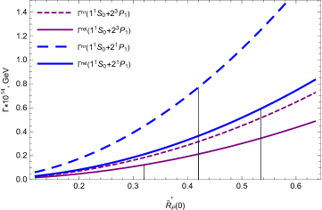
Figure 2: The dependence of the $H$ boson decay width on the value $R^{\prime}_{P}(0)$.

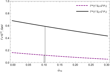
Figure 3: The dependence of the $H$ boson decay width on the value of the largest relativistic parameter $\tilde{\omega}_{10}$.

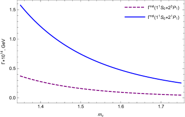
Figure 4: The dependence of the $H$ boson decay width on the value of the c-quark mass.

III Numerical results and conclusion

In this work, we study rare exclusive decays of the Higgs boson into a pair of $B_{c}$ mesons in different S- and P-states. The investigation of various decay channels of the Higgs boson acquired particular relevance after its discovery, although before that, numerous works were carried out to study various mechanisms and decay processes. The study of rare exclusive processes plays an important role in checking the fundamentals of the theory and determining the values of basic parameters. In our work, special attention is paid to relativistic effects connected with taking into account the relative motion of heavy quarks that form $B_{c}$ mesons at the end of the reaction. First, when constructing the Higgs boson decay amplitudes, we take into account the laws of transformation of the relativistic wave functions of mesons and various factors that depend on the relative momenta of the quarks. Then, taking into account the smallness of these relative momenta with respect to the mass of the Higgs boson, some simplifying transformations are made with the extraction of second-order corrections in relative momenta. Relativistic expressions are obtained for the widths of the Higgs boson decay into a pair of different S- and P-wave $B_{c}$ mesons, on the basis of which numerical estimates of these decay widths are made. The decay widths are calculated in the nonrelativistic approximation, and the obtained nonrelativistic results are compared with the results taking into account relativistic effects. We analyzed the dependence of the total decay widths on various sources of relativistic corrections both in the relativistic amplitude of the production of two heavy quarks and antiquarks, and in the operator of the interaction of quarks that compose $B_{c}$ mesons. The role of the main factors $R_{S}(0)$ and $R^{\prime}_{P}(0)$, which affects the numerical results for decay widths, is highlighted. The total degree of these two factors is four, so even a 30 percent decrease in $R_{S}(0)$ and $R^{\prime}_{P}(0)$ leads to a fourfold decrease in the decay widths.

The dependence of the Higgs boson decay width at the production of S- and P-wave $B_{c}$ mesons on the key parameters $R^{\prime}_{P}(0)$, relativistic factor $\tilde{\omega}_{10}$ and the mass of c-quark $m_{1}$ is shown in Fig. 2, Fig. 3, Fig. 4. Our calculations clearly show that taking into account relativistic corrections in the interaction potential of quarks leads to a decrease in the values of $R^{\prime}_{P}(0)$, and, as a consequence, to a decrease in the values of decay widths. When constructing these plots, a fixed value of the wave function at zero for S-states is used. Relativistic corrections in decay amplitudes are determined by $\omega_{ij}$, $\tilde{\omega}_{ij}$ factors. The dependence on the largest relativistic factor $\tilde{\omega}_{10}$ which describes relativistic effects for P-wave mesons is shown in Fig. 3. At the same time, the value of $\omega_{10}$ for S-states was also chosen to be fixed. In this case, there is a decrease in decay widths (some of them are shown in Fig. 3) not exceeding $10\%$. In a separate Fig. 4 the dependence of the calculation results on the c-quark mass for several processes is presented. The obtained numerical values of the decay widths are small in comparison with the total width of Higgs boson $\Gamma=3.2^{+2.8}_{-2.2}\cdot 10^{-3}$ GeV [43]. Therefore, to observe rare decay processes with the formation of a pair of $B_{c}$ mesons, it is necessary to increase the luminosity of the LHC. Possibly that rare decays of the Higgs boson could be investigated at other Higgs factories besides the LHC, such as the ILC (International Linear Collider) and CLIC (Compact Linear Collider) [44].

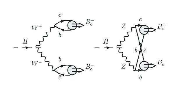
Figure 5: Some amplitudes of the $Z,W$ boson production of a pair of $B_{c}$ mesons in the decay of the Higgs boson.

In this work, a purely quark mechanism for the production of a pair of B mesons in the decay of the H boson is investigated. There are other production mechanisms, which are determined, for example, by the initial decay of the H boson into a pair of ZZ, WW and by other couplings (see Fig. 5). We can obtain an estimate of such contributions using the formalism presented in the previous sections. Considering for definiteness the decay of the Higgs boson into a pair of $ZZ$ with the subsequent production of a pair of pseudoscalar $B_{c}$ mesons, we can represent the width of such a decay in nonrelativistic approximation as follows:

$$\Gamma^{ZZ}_{\cal{PP}}=\frac{\alpha^{3}M_{Z}^{2}M^{3}|\Psi_{\cal P}(0)|^{4}\sqrt{\frac{r_{3}^{2}}{4}-1}}{8\pi M_{H}^{2}(r_{1}^{2}M_{H}^{2}-M_{Z}^{2})(r_{2}^{2}M_{H}^{2}-M_{Z}^{2})\sin^{6}2\theta_{W}}\times$$ (46)

$$\left[1+2a_{c}+2a_{b}-4a_{c}a_{b}-r_{3}^{2}+r_{3}^{2}a_{b}+r_{3}^{2}a_{c}-2r_{3}^{2}a_{c}a_{b}\right]^{2},$$

where $a_{c}=2|q_{c}|\sin^{2}\theta_{W}$, $a_{b}=2|q_{b}|\sin^{2}\theta_{W}$. Numerically, this contribution to the width turns out to be two orders of magnitude smaller than the contribution from the quark decay mechanism studied in this work.

As noted above, for simplicity, when constructing decay amplitudes, we took into account second-order relativistic corrections both in analytical expressions and in numerical calculations, although taking into account corrections of a higher order does not present significant difficulties. The main theoretical errors of the obtained results for decay widths are connected with quark masses, coupling constants, fourth-order corrections in relative momenta $O({\bf p}^{4})$, $O({\bf q}^{4})$ and radiative corrections of order $O(\alpha_{s})$. In the case of production amplitudes for the strong coupling constant $\alpha_{c}$ we use the leading order approximation from (45) where the renormalization scale $\mu=\frac{m_{1}}{m_{1}+m_{2}}M_{H}$ and for $\alpha_{b}$ $\mu=\frac{m_{2}}{m_{1}+m_{2}}M_{H}$. The total theoretical error of the obtained results can be estimated as 40 percent approximately.

Appendix A Explicit form of the functions $f_{i}$, $\tilde{f}_{i}$, $g_{i}$, $\tilde{g}_{i}$ entering the Higgs boson decay widths (30)-(34)

The functions presented here are expressed in terms of mass ratios: $\tilde{r}_{1}=m_{1}/M$, $\tilde{r}_{2}=m_{2}/M$, $r_{5}=M_{2}/M$, $r_{6}=M_{1}/M$, $r_{3}=M_{H}/\sqrt{M_{1}M_{2}}$.

$$f_{1}=-\frac{3}{4}r_{6}+\frac{9}{4}r_{5}+\frac{3}{4}\tilde{r}_{1}\tilde{r}_{2}^{-1}r_{6}+\frac{9}{4}\tilde{r}_{1}\tilde{r}_{2}^{-1}r_{5}+3\tilde{r}_{1}-\frac{3}{2}\tilde{r}_{1}^{2}\tilde{r}_{2}^{-1}-\frac{3}{4}\rho_{1}r_{5}-\frac{3}{4}\rho_{1}\tilde{r}_{1}\tilde{r}_{2}^{-1}r_{5}+\frac{3}{4}\eta_{1}r_{6}-\frac{3}{4}\eta_{1}\tilde{r}_{1}\tilde{r}_{2}^{-1}r_{6},$$ (47)

$$g_{1}=\tilde{\omega}_{\frac{1}{2}\frac{1}{2}}(\frac{3}{2}\tilde{r}_{1})+\tilde{\omega}_{01}(-\frac{3}{4}\tilde{r}_{1}\tilde{r}_{2}^{-1}r_{6}-\frac{9}{4}\tilde{r}_{1}\tilde{r}_{2}^{-1}r_{5}+\frac{3}{2}\tilde{r}_{1}^{2}\tilde{r}_{2}^{-1}+\frac{3}{4}\tilde{r}_{1}^{2}\tilde{r}_{2}^{-1}r_{6}+\frac{3}{4}\tilde{r}_{1}^{2}\tilde{r}_{2}^{-1}r_{5})$$ (48)

$$+\tilde{\omega}_{10}(\frac{3}{4}r_{6}-\frac{9}{4}r_{5}-\frac{3}{2}\tilde{r}_{1}-\frac{3}{4}\tilde{r}_{1}r_{6}+\frac{3}{4}\tilde{r}_{1}r_{5})+\omega_{\frac{1}{2}\frac{1}{2}}(3\tilde{r}_{1})+\omega_{\frac{1}{2}\frac{1}{2}}\tilde{\omega}_{01}(-\frac{3}{2}\tilde{r}_{1})+\omega_{\frac{1}{2}\frac{1}{2}}\tilde{\omega}_{10}(-\tilde{r}_{1})+$$

$$\omega_{01}(-\frac{1}{4}r_{6}+\frac{3}{4}r_{5}-\tilde{r}_{1}+\frac{1}{4}\tilde{r}_{1}r_{6}-\frac{1}{4}\tilde{r}_{1}r_{5})+\omega_{01}\tilde{\omega}_{01}(\frac{1}{4}r_{6}-\frac{3}{4}r_{5}+\tilde{r}_{1}-\frac{1}{4}\tilde{r}_{1}r_{6}+\frac{1}{4}\tilde{r}_{1}r_{5})$$

$$+\omega_{10}(\frac{1}{4}\tilde{r}_{1}\tilde{r}_{2}^{-1}r_{6}+\frac{3}{4}\tilde{r}_{1}\tilde{r}_{2}^{-1}r_{5}-\frac{3}{2}\tilde{r}_{1}-\frac{1}{4}\tilde{r}_{1}^{2}\tilde{r}_{2}^{-1}r_{6}-\frac{1}{4}\tilde{r}_{1}^{2}\tilde{r}_{2}^{-1}r_{5})+$$

$$\omega_{10}\tilde{\omega}_{01}(\frac{1}{2}\tilde{r}_{1})+\omega_{10}\tilde{\omega}_{10}(-\frac{1}{4}\tilde{r}_{1}\tilde{r}_{2}^{-1}r_{6}-\frac{3}{4}\tilde{r}_{1}\tilde{r}_{2}^{-1}r_{5}+\frac{3}{2}\tilde{r}_{1}+\frac{1}{4}\tilde{r}_{1}^{2}\tilde{r}_{2}^{-1}r_{6}+\frac{1}{4}\tilde{r}_{1}^{2}\tilde{r}_{2}^{-1}r_{5}),$$

$$f_{2}=\frac{3}{4}r_{6}-\frac{1}{4}r_{5}-\frac{3}{4}\tilde{r}_{1}\tilde{r}_{2}^{-1}r_{6}-\frac{1}{4}\tilde{r}_{1}\tilde{r}_{2}^{-1}r_{5}-\tilde{r}_{1}+\frac{1}{2}\tilde{r}_{1}^{2}\tilde{r}_{2}^{-1}+\frac{1}{4}\rho_{1}r_{5}+\frac{1}{4}\rho_{1}\tilde{r}_{1}\tilde{r}_{2}^{-1}r_{5}-\frac{1}{4}\eta_{1}r_{6}+\frac{1}{4}\eta_{1}\tilde{r}_{1}\tilde{r}_{2}^{-1}r_{6},$$ (49)

$$g_{2}=\tilde{\omega}_{\frac{1}{2}\frac{1}{2}}(-\frac{1}{2}\tilde{r}_{1})+\tilde{\omega}_{01}(\frac{3}{4}\tilde{r}_{1}\tilde{r}_{2}^{-1}r_{6}+\frac{1}{4}\tilde{r}_{1}\tilde{r}_{2}^{-1}r_{5}-\frac{1}{2}\tilde{r}_{1}^{2}\tilde{r}_{2}^{-1}-\frac{1}{4}\tilde{r}_{1}^{2}\tilde{r}_{2}^{-1}r_{6}-\frac{1}{4}\tilde{r}_{1}^{2}\tilde{r}_{2}^{-1}r_{5})+\tilde{\omega}_{10}(-\frac{3}{4}r_{6}+\frac{1}{4}r_{5}+$$ (50)

$$\frac{1}{2}r_{1}+\frac{1}{4}\tilde{r}_{1}r_{6}-\frac{1}{4}\tilde{r}_{1}r_{5})+\omega_{\frac{1}{2}\frac{1}{2}}(\tilde{r}_{1})+\omega_{\frac{1}{2}\frac{1}{2}}\tilde{\omega}_{01}(\frac{1}{2}\tilde{r}_{1})+\omega_{\frac{1}{2}\frac{1}{2}}\tilde{\omega}_{10}(-\tilde{r}_{1})+\omega_{01}(-\frac{3}{4}r_{6}+\frac{1}{4}r_{5}-\tilde{r}_{1}+\frac{1}{4}\tilde{r}_{1}r_{6}-$$

$$\frac{1}{4}\tilde{r}_{1}r_{5})+\omega_{01}\tilde{\omega}_{01}(\frac{3}{4}r_{6}-\frac{1}{4}r_{5}+\tilde{r}_{1}-\frac{1}{4}\tilde{r}_{1}r_{6}+\frac{1}{4}\tilde{r}_{1}r_{5})+\omega_{10}(\frac{3}{4}\tilde{r}_{1}\tilde{r}_{2}^{-1}r_{6}+\frac{1}{4}\tilde{r}_{1}\tilde{r}_{2}^{-1}r_{5}+\frac{1}{2}\tilde{r}_{1}-\frac{1}{4}\tilde{r}_{1}^{2}\tilde{r}_{2}^{-1}r_{6}-$$

$$\frac{1}{4}\tilde{r}_{1}^{2}\tilde{r}_{2}^{-1}r_{5})+\omega_{10}\tilde{\omega}_{01}(\frac{1}{2}\tilde{r}_{1})+\omega_{10}\tilde{\omega}_{10}(-\frac{3}{4}\tilde{r}_{1}\tilde{r}_{2}^{-1}r_{6}-\frac{1}{4}\tilde{r}_{1}\tilde{r}_{2}^{-1}r_{5}-\frac{1}{2}\tilde{r}_{1}+\frac{1}{4}\tilde{r}_{1}^{2}\tilde{r}_{2}^{-1}r_{6}+\frac{1}{4}\tilde{r}_{1}^{2}\tilde{r}_{2}^{-1}r_{5}),$$

$$f_{3}=-\frac{1}{4}r_{6}-\frac{1}{4}r_{5}-\frac{1}{4}\tilde{r}_{1}\tilde{r}_{2}^{-1}r_{6}+\frac{1}{4}\tilde{r}_{1}\tilde{r}_{2}^{-1}r_{5}),$$ (51)

$$g_{3}=\tilde{\omega}_{01}(\frac{1}{4}\tilde{r}_{1}\tilde{r}_{2}^{-1}r_{6}-\frac{1}{4}\tilde{r}_{1}\tilde{r}_{2}^{-1}r_{5})+\tilde{\omega}_{10}(\frac{1}{4}r_{6}+\frac{1}{4}r_{5})+\omega_{01}(-\frac{1}{12}r_{6}-\frac{1}{12}r_{5})+\omega_{01}\tilde{\omega}_{01}(\frac{1}{12}r_{6}+\frac{1}{12}r_{5})$$ (52)

$$+\omega_{10}(-\frac{1}{12}\tilde{r}_{1}\tilde{r}_{2}^{-1}r_{6}+\frac{1}{12}\tilde{r}_{1}\tilde{r}_{2}^{-1}r_{5})+\omega_{10}\tilde{\omega}_{10}(\frac{1}{12}\tilde{r}_{1}\tilde{r}_{2}^{-1}r_{6}-\frac{1}{12}\tilde{r}_{1}\tilde{r}_{2}^{-1}r_{5}),$$

$$f_{4}=\frac{3}{4}r_{6}-\frac{1}{4}r_{5}-\frac{3}{4}\tilde{r}_{1}\tilde{r}_{2}^{-1}r_{6}-\frac{1}{4}\tilde{r}_{1}\tilde{r}_{2}^{-1}r_{5}-\tilde{r}_{1}+\frac{1}{2}\tilde{r}_{1}^{2}\tilde{r}_{2}^{-1}+\frac{1}{4}\rho_{1}r_{5}+\frac{1}{4}\rho_{1}\tilde{r}_{1}\tilde{r}_{2}^{-1}r_{5}-\frac{1}{4}\eta_{1}r_{6}+\frac{1}{4}\eta_{1}\tilde{r}_{1}\tilde{r}_{2}^{-1}r_{6},$$ (53)

$$g_{4}=\tilde{\omega}_{\frac{1}{2}\frac{1}{2}}(-\frac{1}{2}\tilde{r}_{1})+\tilde{\omega}_{01}(\frac{3}{4}\tilde{r}_{1}\tilde{r}_{2}^{-1}r_{6}+\frac{1}{4}\tilde{r}_{1}\tilde{r}_{2}^{-1}r_{5}-\frac{1}{2}\tilde{r}_{1}^{2}\tilde{r}_{2}^{-1}-\frac{1}{4}\tilde{r}_{1}^{2}\tilde{r}_{2}^{-1}r_{6}-\frac{1}{4}\tilde{r}_{1}^{2}\tilde{r}_{2}^{-1}r_{5})+$$ (54)

$$\tilde{\omega}_{10}(-\frac{3}{4}r_{6}+\frac{1}{4}r_{5}+\frac{1}{2}\tilde{r}_{1}+\frac{1}{4}\tilde{r}_{1}r_{6}-\frac{1}{4}\tilde{r}_{1}r_{5})+\omega_{\frac{1}{2}\frac{1}{2}}(\tilde{r}_{1})+\omega_{\frac{1}{2}\frac{1}{2}}\tilde{\omega}_{01}(\frac{1}{2}\tilde{r}_{1})+\omega_{\frac{1}{2}\frac{1}{2}}\tilde{\omega}_{10}(-\tilde{r}_{1})+$$

$$\omega_{01}(-\frac{3}{4}r_{6}+\frac{1}{4}r_{5}-\tilde{r}_{1}+\frac{1}{4}\tilde{r}_{1}r_{6}-\frac{1}{4}\tilde{r}_{1}r_{5})+\omega_{01}\tilde{\omega}_{01}(\frac{3}{4}r_{6}-\frac{1}{4}r_{5}+\tilde{r}_{1}-\frac{1}{4}\tilde{r}_{1}r_{6}+\frac{1}{4}\tilde{r}_{1}r_{5})+$$

$$\omega_{10}(\frac{3}{4}\tilde{r}_{1}\tilde{r}_{2}^{-1}r_{6}+\frac{1}{4}\tilde{r}_{1}\tilde{r}_{2}^{-1}r_{5}+\frac{1}{2}r_{1}-\frac{1}{4}\tilde{r}_{1}^{2}\tilde{r}_{2}^{-1}r_{6}-\frac{1}{4}\tilde{r}_{1}^{2}\tilde{r}_{2}^{-1}r_{5})+\omega_{10}\tilde{\omega}_{01}(\frac{1}{2}\tilde{r}_{1})$$

$$+\omega_{10}\tilde{\omega}_{10}(-\frac{3}{4}\tilde{r}_{1}\tilde{r}_{2}^{-1}r_{6}-\frac{1}{4}\tilde{r}_{1}\tilde{r}_{2}^{-1}r_{5}-\frac{1}{2}\tilde{r}_{1}+\frac{1}{4}\tilde{r}_{1}^{2}\tilde{r}_{2}^{-1}r_{6}+\frac{1}{4}\tilde{r}_{1}^{2}\tilde{r}_{2}^{-1}r_{5}),$$

$$f_{5}=-\frac{3}{2}r_{6}+\frac{1}{2}r_{5}-\frac{3}{2}\tilde{r}_{1}\tilde{r}_{2}^{-1}r_{6}-\frac{1}{2}\tilde{r}_{1}\tilde{r}_{2}^{-1}r_{5}+2r_{1}+\tilde{r}_{1}^{2}\tilde{r}_{2}^{-1}-\frac{1}{2}\rho_{1}r_{5}+\frac{1}{2}\rho_{1}\tilde{r}_{1}\tilde{r}_{2}^{-1}r_{5}+\frac{1}{2}\eta_{1}r_{6}+\frac{1}{2}\eta_{1}\tilde{r}_{1}\tilde{r}_{2}^{-1}r_{6},$$ (55)

$$g_{5}=\tilde{\omega}_{\frac{1}{2}\frac{1}{2}}(-\tilde{r}_{1})+\tilde{\omega}_{01}(\frac{3}{2}\tilde{r}_{1}\tilde{r}_{2}^{-1}r_{6}+\frac{1}{2}\tilde{r}_{1}\tilde{r}_{2}^{-1}r_{5}-\tilde{r}_{1}^{2}\tilde{r}_{2}^{-1}-\frac{1}{2}\tilde{r}_{1}^{2}\tilde{r}_{2}^{-1}r_{6}-\frac{1}{2}\tilde{r}_{1}^{2}\tilde{r}_{2}^{-1}r_{5})+$$ (56)

$$\tilde{\omega}_{10}(\frac{3}{2}r_{6}-\frac{1}{2}r_{5}-\tilde{r}_{1}-\frac{1}{2}\tilde{r}_{1}r_{6}+\frac{1}{2}\tilde{r}_{1}r_{5})+\omega_{\frac{1}{2}\frac{1}{2}}(-4\tilde{r}_{1})+\omega_{\frac{1}{2}\frac{1}{2}}\tilde{\omega}_{01}(\tilde{r}_{1})+\omega_{\frac{1}{2}\frac{1}{2}}\tilde{\omega}_{10}(2\tilde{r}_{1})+$$

$$\omega_{01}(-\frac{3}{2}r_{6}+\frac{1}{2}r_{5}-2\tilde{r}_{1}+\frac{1}{2}\tilde{r}_{1}r_{6}-\frac{1}{2}\tilde{r}_{1}r_{5})+\omega_{01}\tilde{\omega}_{01}(\frac{3}{2}r_{6}-\frac{1}{2}r_{5}+2\tilde{r}_{1}-\frac{1}{2}\tilde{r}_{1}r_{6}+\frac{1}{2}\tilde{r}_{1}r_{5})+$$

$$\omega_{10}(-\frac{3}{2}\tilde{r}_{1}\tilde{r}_{2}^{-1}r_{6}-\frac{1}{2}\tilde{r}_{1}\tilde{r}_{2}^{-1}r_{5}-r_{1}+\frac{1}{2}\tilde{r}_{1}^{2}\tilde{r}_{2}^{-1}r_{6}+\frac{1}{2}\tilde{r}_{1}^{2}\tilde{r}_{2}^{-1}r_{5})+\omega_{10}\tilde{\omega}_{01}(\tilde{r}_{1})+$$

$$\omega_{10}\tilde{\omega}_{10}(\frac{3}{2}\tilde{r}_{1}\tilde{r}_{2}^{-1}r_{6}+\frac{1}{2}\tilde{r}_{1}\tilde{r}_{2}^{-1}r_{5}+\tilde{r}_{1}-\frac{1}{2}\tilde{r}_{1}^{2}\tilde{r}_{2}^{-1}r_{6}-\frac{1}{2}\tilde{r}_{1}^{2}\tilde{r}_{2}^{-1}r_{5}).$$

The functions $\tilde{f}_{i}$, $\tilde{g}_{i}$ can be obtained from $f_{i}$, $g_{i}$ as a result of the replacement $\tilde{r}_{1}\leftrightarrow\tilde{r}_{2}$, $\tilde{\omega}_{ij}\leftrightarrow\tilde{\omega}_{ji}$.

Appendix B The construction of an effective Hamiltonian

Using potential (41), we construct an effective model of the quark interaction of the Schrödinger-type and calculate the relativistic parameters included in the decay widths. The first step in the construction of the model is related to the rationalization of the kinetic energy operator as follows:

$$T=\sqrt{{\bf p}^{2}+m_{1}^{2}}-m_{1}+\sqrt{{\bf p}^{2}+m_{2}^{2}}-m_{2}=\frac{{\bf p}^{2}}{\sqrt{{\bf p}^{2}+m_{1}^{2}}+m_{1}}+\frac{{\bf p}^{2}}{\sqrt{{\bf p}^{2}+m_{2}^{2}}+m_{2}}\approx$$ (57)

$$\frac{{\bf p}^{2}}{E_{1}+m_{1}}+\frac{{\bf p}^{2}}{E_{2}+m_{2}}=\frac{{\bf p}^{2}}{2\tilde{m}_{1}}+\frac{{\bf p}^{2}}{2\tilde{m}_{2}}=\frac{{\bf p}^{2}}{2\tilde{\mu}},$$

where we change relativistic particle energies $\varepsilon_{1,2}({\bf p})$ by their effective values $E_{1,2}$ so that $M_{B_{c}}=E_{1}+E_{2}$ or what is the same ${\bf p}^{2}\to{\bf p}^{2}_{eff}$. The effective quark masses $\tilde{m}_{1,2}$ are used further in the program for the numerical solution of the Schrödinger equation. ${\bf p}^{2}_{eff}$ should be considered as a new parameter which effectively accounts for relativistic corrections.

Another part of the relativistic corrections in the Breit Hamiltonian is determined by the term:

$$\Delta\tilde{U}=-\frac{2\alpha_{s}}{3m_{1}m_{2}r}\left[{\bf p}^{2}-\frac{d^{2}}{dr^{2}}\right].$$ (58)

In order to replace it by the effective term containing the power-like potentials, we use the approximate bound state wave functions which can be written for S- and P-wave states as follows:

$$\Psi_{\cal S}({\bf r})=\frac{\beta^{3/2}}{\pi^{3/4}}e^{-\frac{1}{2}\beta^{2}r^{2}},~{}~{}\Psi_{\cal P}({\bf r})=\sqrt{\frac{8}{3}}\frac{\beta^{3/2}}{\pi^{3/4}}\beta re^{-\frac{1}{2}\beta^{2}r^{2}}Y_{1m}(\theta,\phi).$$ (59)

The parameter $\beta$ entering here is chosen in such a way that the calculated value of $R_{S}(0)$ and $R^{\prime}_{P}(0)$ is obtained. The operator ${\bf p}^{2}$ is changed by its nonrelativistic expression: ${\bf p}^{2}=2\mu\left(E_{nr}+\frac{4\alpha_{s}}{3r}-Ar-B\right)$, where nonrelativistic energy $E_{nr}$ is obtained by the numerical solution of the Schrödinger equation in the nonrelativistic approximation.

In the case of S-wave states it is necessary to change the $\delta$-like term of the potential by known smeared $\delta$-function of the Gaussian form:

$$\tilde{\delta}({\bf r})=\frac{b^{3}}{\pi^{3/2}}e^{-b^{2}r^{2}}$$ (60)

with the additional parameter $b$ which defines the hyperfine splitting in the $(b\bar{c})$ system.

The second step in constructing an effective model of quark interaction is connected with the angular averaging of the spin-orbit and spin-spin terms. This averaging is performed separately for the considered S- and P-states [45]. In this case, we use a basis transformation of the following form:

$$\Psi_{SLFM_{F}}=\sum_{J}(-1)^{s_{1}+s_{2}+L+F}\sqrt{(2S+1)(2J+1)}\Biggl{\{}\begin{array}[]{ccc}L&~{}s_{1}&~{}J\\ s_{2}&~{}F&~{}S\end{array}\Biggr{\}}\Psi_{Js_{2}FM_{F}},$$ (61)

where ${\bf J}={\bf L}+{\bf s_{1}}$ is the total nomentum of quark 1, ${\bf S}={\bf s}_{1}+{\bf s}_{2}$, ${\bf F}={\bf S}+{\bf L}={\bf J}+{\bf s}_{2}$. For diagonal matrix elements we have the expression:

$$<Js_{2}FM_{F}|[({\bf L}{\bf s}_{2})+3({\bf s}_{1}{\bf n})({\bf s}_{2}{\bf n})-({\bf s}_{1}{\bf s}_{2})]|Js_{2}FM_{F}>=\frac{L(L+1)}{J(J+1)}[F(F+1)-J(J+1)-s_{2}(s_{2}+1)].$$ (62)

The matrix elements of the spin-orbit $T_{1}={\bf L}{\bf s}_{2}$ and spin-spin interactions $T_{2}=3({\bf s}_{1}{\bf n})({\bf s}_{2}{\bf n})-({\bf s}_{1}{\bf s}_{2})$ off-diagonal in $J$ with $F=1$ are determined as follows:

$$<J^{\prime}s_{2}FM_{F}|T_{1}|Js_{2}FM_{F}>=(-1)^{-J-F-s_{2}+L+3/2+J^{\prime}}\sqrt{(2J^{\prime}+1)(2J+1)}\times$$ (63)

$$\sqrt{(2s_{2}+1)(s_{2}+1)s_{2}(2L+1)(L+1)L}\Biggl{\{}\begin{array}[]{ccc}J&~{}s_{2}&~{}F\\ s_{2}&~{}J^{\prime}&~{}1\end{array}\Biggr{\}}\Biggl{\{}\begin{array}[]{ccc}L&~{}J^{\prime}&~{}1/2\\ J&~{}L&~{}1\end{array}\Biggr{\}}.$$

As a result $<J^{\prime}s_{2}FM_{F}|T_{1}|Js_{2}FM_{F}>=2<J^{\prime}s_{2}FM_{F}|T_{2}|Js_{2}FM_{F}>=-\frac{\sqrt{2}}{3}$. After angular averaging an effective Hamiltonians are obtained describing the states ${}^{3}S_{1}$, ${}^{1}S_{0}$, ${}^{3}P_{J}$, ${}^{1}P_{1}$.

Finally, the third final step is related to the numerical solution of the Schrödinger equation with obtained effective Hamiltonians. We use a calculation program in the system Mathematica [42]. The obtained numerical results are presented in Table 1. They are in good agreement with previous calculations [32, 35, 36].

References

• [1] G. Aad et al. [the ATLAS Collaboration], Phys. Lett. B 716, 1 (2012).
• [2] S. Chartchyan et al. [the CMS Collaboration], Phys. Lett. B 716, 30 (2012).
• [3] W. J. Keung, Phys. Rev. D 27, 2762 (1983).
• [4] M. A. Shifman and M. I. Vysotsky, Nucl. Phys. B 186, 475 (1981).
• [5] G. T. Bodwin, H. S. Chung, J.-H. Ee, J. Lee and F. Petriello, Phys. Rev. D 90, 113010 (2014).
• [6] V. Kartvelishvili, A. V. Luchinsky, and A. A. Novoselov, Phys. Rev. D 79, 114015 (2009).
• [7] J. Jiang and C.-F. Qiao, Phys. Rev. D 93, 054031 (2016).
• [8] J.-J. Niu, L.  Guo, H.-H. Ma, X.-G. Wu, Eur. Phys. J. C 79, 339 (2019).
• [9] A. L. Kataev and V. T. Kim, Mod. Phys. Lett. A 9, 1309 (1994).
• [10] I. N. Belov, A. V. Berezhnoy, A. E. Dorokhov et al., Nucl. Phys. A 1015, 122285 (2021).
• [11] A. E. Dorokhov, R. N. Faustov, A. P. Martynenko, and F .A. Martynenko, Phys. Rev. D 102, 016027 (2020).
• [12] E. N. Elekina and A. P. Martynenko, Phys. Rev. D 81, 054006 (2010).
• [13] A. P. Martynenko and A. M. Trunin, Phys. Rev. D 86, 094003 (2012).
• [14] N. Brambilla, S. Eidelman, B.K. Heltsley et al. Eur. Phys. J. C 71, 1534 (2011).
• [15] G. Aad et al. [the ATLAS Collaboration], Physical Review D 90, 112015 (2014).
• [16] G. Aad et al. [the ATLAS Collaboration], JHEP 08, 137 (2015).
• [17] A. M. Sirunyan et al. [the CMS Collaboration], Phys. Rev. Lett. B 797, 121801 (2018).
• [18] S. Chatrchyan et al. [the CMS Collaboration], JHEP 05, 104 (2014).
• [19] A. M. Sirunyan et al. [the CMS Collaboration], Phys. Lett. B 797, 134811 (2019).
• [20] A. V. Berezhnoy, I. N. Belov, A. K. Likhoded and, A. V. Luchinsky, Mod. Phys. Lett. A 34, 40 (2019).
• [21] A. V. Berezhnoy, A. P. Martynenko and F. A. Martynenko and O. S. Sukhorukova, Nucl. Phys. A 986, 34 (2019).
• [22] A. A. Karyasov, A. P. Martynenko and F. A. Martynenko, Nucl. Phys. B 911, 36 (2016).
• [23] G. T. Bodwin and A. Petrelli, Phys. Rev. D 66, 094011 (2002).
• [24] S. J. Brodsky and J. R. Primack, Ann. Phys. 52, 315 (1969).
• [25] R. N. Faustov, Ann. Phys. 78, 176 (1973).
• [26] J. Kuipers, T. Ueda, J. A. M. Vermaseren, and J. Vollinga, Comput. Phys. Commun. 184, 1453 (2013).
• [27] G. T. Bodwin, E. Braaten and G. P. Lepage, Phys. Rev. D 51, 1125 (1995).
• [28] S. N. Gupta, S. F. Radford and W. W. Repko, Phys. Rev. D 26, 3305 (1982).
• [29] N. Brambilla, A. Pineda, J. Soto and A. Vairo, Rev. Mod. Phys. 77, 1423 (2005).
• [30] S. Capstick and N. Isgur, Phys. Rev. D 34, 2809 (1986).
• [31] S. Godfrey and N. Isgur, Phys. Rev. D 32, 189 (1985).
• [32] S. S. Gershtein, V. V. Kiselev, A. K. Likhoded, and A. V. Tkabladze, Phys. Usp. 38, 1 (1995).
• [33] S. Godfrey, Phys. Rev. D 70, 054017 (2004).
• [34] W. Lucha and F. F. Schöberl, Phys. Rev. A 51, 4419 (1995).
• [35] D. Ebert, R. N. Faustov and V. O. Galkin, Phys. Rev. D 67, 014027 (2003).
• [36] D. Ebert, R. N. Faustov and V. O. Galkin, Eur. Phys. J. C 71, 1825 (2011).
• [37] D. Ebert, R. N. Faustov, V. O. Galkin and A. P. Martynenko, Phys. Atom. Nucl. 68, 784 (2005).
• [38] S. F. Radford and W. W. Repko, Phys. Rev. D 75, 074031 (2007).
• [39] S. N. Gupta, Phys. Rev. D 35, 1736 (1987).
• [40] S. N. Gupta, J. M. Johnson, W. W. Repko and C. J. Suchyta, Phys. Rev. D 49, 1551 (1994).
• [41] K. G. Chetyrkin, B. A. Kniehl and M. Steinhauser, Phys. Rev. Lett. 79, 2184 (1997).
• [42] W. Lucha and F. F. Schöberl, Int. J. Mod. Phys. C 10, 607 (1999).
• [43] P. A. Zyla et al. (Particle Data Group), Prog. Theor. Exp. Phys. 2020, 083C01 (2020).
• [44] J. de Blas, R. Franceschini, F. Riva, P. Roloff, U. Schnoor et al., CERN Yellow Rep. Monogr. Vol. 3 (2018); arXiv:1812.02093 [hep-ph].
• [45] V. K. Khersonsky, E. V. Orlenko and D. A. Varshalovich,, Quantum theory of angular momentum and its applications Vol.2, M., Nauka, 2017.