Influence Selection for Active Learning

Abstract

The existing active learning methods select the samples by evaluating the sample’s uncertainty or its effect on the diversity of labeled datasets based on different task-specific or model-specific criteria. In this paper, we propose the Influence Selection for Active Learning(ISAL) which selects the unlabeled samples that can provide the most positive Influence on model performance. To obtain the Influence of the unlabeled sample in the active learning scenario, we design the Untrained Unlabeled sample Influence Calculation(UUIC) to estimate the unlabeled sample’s expected gradient with which we calculate its Influence. To prove the effectiveness of UUIC, we provide both theoretical and experimental analyses. Since the UUIC just depends on the model gradients, which can be obtained easily from any neural network, our active learning algorithm is task-agnostic and model-agnostic. ISAL achieves state-of-the-art performance in different active learning settings for different tasks with different datasets. Compared with previous methods, our method decreases the annotation cost at least by 12%, 13% and 16% on CIFAR10, VOC2012 and COCO, respectively.

1 Introduction

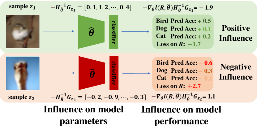
Figure 1: Using UUIC to calculate the influence of unlabeled samples. These two samples will be annotated as ’Bird’ if they are selected. In UUIC, we calculate the influence of the sample by calculating $-\nabla_{\theta}l(R,\hat{\theta})^{T}H_{\hat{\theta}}^{-1}G_{z_{i}}$. The more negative the influence value is, the more positive influence on model performance the sample provides. Base on the result from UUIC, our ISAL algorithm selects the sample $z_{1}$ for annotation.

Active learning is a kind of sampling algorithm that aims to reduce the annotation cost by helping the model to achieve better performance with fewer labeled training samples. In those areas with a limited annotation budget or the areas that need large amounts of labeled samples, active learning plays an important and irreplaceable role. However, unlike the rapid progress of weakly supervised learning and semi-supervised learning, the development of active learning is limited. Especially in the computer vision area, most of the existing active learning algorithms are restricted to the image classification problem.

Given a pool of unlabeled images, different active learning algorithms evaluate the importance of each image with different criteria, which can be divided into uncertainty-based methods and diversity-based methods. The uncertainty-based methods [19, 14, 34, 8, 40] use different criteria to evaluate the uncertainty of an image and select the images that the trained model is less confident about. However, the neural network shows over-confidence [13] toward the unfamiliar samples, indicating that using the uncertainty to estimate the samples’ importance may not be accurate, deteriorating the performance of the active learning algorithm.

The diversity-based methods [24, 39, 10, 31] aim to select a subset from the whole unlabeled dataset with the largest diversity. These methods do not consider the model state. Besides, some of them need to measure the distance between each labeled image and each unlabeled image, meaning that their computation complexity are quadratic with respect to the size of the dataset. This disadvantage will become more apparent on the large-scale dataset.

In addition to image classification, object detection is also an important area that has large amounts of applications. The annotation for the datasets  [20, 35, 6] of object detection is extremely time-consuming. Thus, active learning for object detection is well demanded. However, the research in active learning for object detection [30, 15, 4, 11] is rare and most of the proposed methods are designed for specific architecture, e.g., Faster R-CNN [27] or SSD [21].

In this paper, instead of designing a task or even architecture-specific algorithms, we propose an algorithm that can be generally applied to different tasks and architectures. There are already some successful attempts like the diversity-based coreset [31] and the uncertainty-based learning loss [40] algorithm, which proves that the general algorithm for active learning is possible. Unlike these two algorithms that select samples by measuring the feature distance or the expected loss which are assumed to be correlated with the potential influence on the model, our method estimates the samples’ influence directly.

Our method, Influence Selection for Active Learning(ISAL), selects samples with the most positive influence, i.e. the model performance will be enhanced most by adding this sample with full annotation into the labeled dataset. The influence measurement was first proposed by Cook [3] for robust statistics. However, the scenario for the influence estimation in our work is entirely different. In our case, the samples are unlabeled and untrained. We design the Untrained Unlabeled sample Influence Calculation(UUIC) to calculate the influence of the unlabeled and untrained sample by estimating its expected gradient. Figure. 1 shows how UUIC evaluates unlabeled samples and helps ISAL select samples. Since UUIC just needs to use the model gradients, which can be easily obtained in a neural network no matter what task is and how complex the model structure is, our proposed ISAL is task-agnostic and model-agnostic.

ISAL achieves state-of-the-art performance among all comparing active learning algorithms for both the image classification and object detection task in the commonly used active learning setting with different representative datasets. Our method saves 12%, 13%, 16% annotation than the best comparing methods in CIFAR10 [17], VOC2012 [6] and COCO [20], respectively. In addition, the existing methods for object detection perform better than random sampling only when the trained model’s performance is far lower than the ones trained on the full dataset, indicating that some selected samples may not be the best choice. Thus, we apply ISAL to a large-scale active learning setting for object detection. ISAL decreases the annotation cost at least by 8% than all comparing methods when the detector reaches 94.4% performance of the model trained on the full COCO dataset.

The contribution of this paper is summarized as follows:

1. We propose Influence Selection for Active Learning(ISAL), a task-agnostic and model-agnostic active learning algorithm, which selects samples based on the calculated influence.

2. We design the Untrained Unlabeled sample Influence Calculation(UUIC), a method to calculate the influence of the unlabeled and untrained sample by estimating its expected gradient. To validate UUIC’s effectiveness, we provide both theoretical and experimental analyses.

3. ISAL achieves state-of-the-art performance in different experiment settings for both image classification and object detection.

2 Related Work

The existing active learning methods [26] can be divided into two categories: uncertainty-based and diversity-based methods. Many of them are designed for image classification or can be used in classification without much change.

Uncertainty-based Methods. The uncertainty has been widely used in active learning to estimate samples’ importance. It can be defined as the posterior probability of a predicted class [19, 18, 38], the posterior probability margin between the first and the second predicted class [14, 29], or the entropy of the posterior probability distribution [32, 14, 22, 33]. In addition to directly using the posterior probability, researchers design some different methods for evaluating the samples’ uncertainty. Seung [34] trains multiple models to construct a committee and measures uncertainty by the consensus between the multiple predictions from the committee. Gal [8] proposes an active learning method that obtains uncertainty estimation through multiple forward passes with Monte Carlo Dropout. Yoo [40] creates a module that learns how to predict the unlabeled images’ loss and chooses the unlabeled image with the highest predicted loss. Freytag [7] selects the images with the biggest expected model output changes, which can be also regarded as the uncertainty-based method.

Diversity-based Method. It aims to solve the sampling bias problem in batch querying. To achieve this goal, a clustering algorithm is applied [24] or a discrete optimization problem [39, 5, 9] is solved. The core-set approach [31] attempts to solve this problem by constructing a core subset. In addition to using k-Center-Greedy to calculate the core subset, its performance can be further enhanced by solving a mixed-integer program. The context-aware methods [10, 23] consider the distance between the samples and their surrounding points to enrich the diversity of the labeled dataset. Sinha [36] trains a variational autoencoder and an adversarial network to discriminate between unlabeled and labeled samples, which can also be regarded as a diversity-based method.

Active Learning for Object Detection. The research in active learning for object detection is rare and most of the existing methods need complicated design. Roy [30] selects the images with the biggest offset between the bounding boxes(bboxes) predicted in intermediate layers and the last layer of the SSD [21] model. Kao [15] proposes to use the intersection over union(IoU) between the bboxes predicted by the Region Proposal Network(RPN) head and Region of Interest(RoI) head of Faster R-CNN [27] to measure the image uncertainty, or measuring the uncertainty of an image by the change of the predicted bboxes under different levels of data augmentation, and chooses the images with the highest uncertainty. Desai [4] measures the bbox-level uncertainty and proposes a new method that chooses bboxes for active learning instead of images. Haussmann [11] examines different existing methods in the scenario of large-scale active learning for object detection. He finds that the method which achieves the best performance chooses the images with more bboxes, increasing the annotation cost which is contradictory to the purpose of the active learning. In fact, most of the researches ignore that the annotation cost of object detection is closely relative to the bboxes number instead of the image number.

Influence Function. Cook [3] first introduces influence function for robust statistics. The influence function evaluates the importance of a trained sample by measuring how the model parameters change as we upweight this sample by an infinitesimal amount. Recently, Koh [16] uses the influence function to understand the neural network model behavior. Ren [28] evaluates the trained unlabeled sample in semi-supervised learning by influence function. However, as far as we know, none of the existing publications uses the influence function on the untrained sample. Besides, Cook’s derivation of influence function is also based on the trained sample. Thus there is no solid theoretical support for using the influence function on the untrained sample so far.

3 Method

In this section, we start with the problem definition of active learning. In Section 3.2, we provide a derivation for evaluating the influence of an untrained sample. In Section 3.3, we introduce Untrained Unlabeled sample Influence Calculation(UUIC) to estimate an untrained unlabeled sample’s expected gradient with which we calculate the influence of this sample. In Section 3.4, we show our proposed Influence Selection for Active Learning algorithm.

3.1 Problem Definition

In this section, we formally define the problem of active learning. We focus on some traditional computer vision tasks such as image classification and object detection.

In real-world setting, we gather a large pool of unlabeled samples $U_{0}$. We randomly select a small amount of samples $S_{0}$ from $U_{0}$ and annotate them, the $U_{1}=U_{0}\setminus S_{0}$. The $S_{0}$ will be split into two parts, the initial labeled samples $L_{1}$, and the validation set $V$, which will be used to measure the trained model performance. The $L_{1}$ will be used to train the first model $M_{1}$ in active learning iteration. Then all unlabeled samples in $U_{1}$ will be evaluated according to some specific criteria. In our proposed method, we calculate the unlabeled sample’s influence on model performance and use influence value as the criterion to evaluate the importance of the untrained sample. Based on the evaluation result, a new group of unlabeled samples $S_{1}$ will be selected and annotated. The labeled and unlabeled dataset will be updated, $U_{2}=U_{1}\setminus S_{1}$, and the $L_{2}=L_{1}\cup S_{1}$. Then $L_{2}$ will be used to train another model $M_{2}$, and $U_{2}$ will be evaluated and $S_{2}$ will be selected. This iteration will be repeated until the model achieves a satisfactory performance on $V$ or until we have exhausted the budget for annotation. Fig. 2 shows the pipeline of active learning.

Figure 2: The pipeline of active learning. The iteration will be repeated until the model achieves a satisfactory performance or until we have exhausted the budget for annotation.

3.2 The Influence of an Untrained Sample

In each step of the active learning, except the initial step, we have an unlabeled dataset $U_{i}$ and a labeled dataset $L_{i}$. With all the samples in $L_{i}=\{z_{1},z_{2},\cdots,z_{n}\}$ and loss function $\mathcal{L}(\theta)=\frac{1}{n}{\textstyle\sum_{j=1}^{n}}l(z_{j},\theta)$, we train a model with its parameters $\theta\in\Theta$. The model would converge to $\hat{\theta}\in\Theta$, where $\hat{\theta}\overset{def}{=}\arg\min\;_{\theta\in\Theta}\;\frac{1}{n}{\textstyle\sum_{j=1}^{n}}l(z_{j},\theta)$.

Next, we need to evaluate each unlabeled sample and select the most useful samples. We first measure the model parameters change due to adding a new sample $z^{{}^{\prime}}\in U_{i}$ into the labeled dataset. We evaluate $z^{{}^{\prime}}$ with the assumption that we already have its ground truth label. The change of the parameter is $\hat{\theta}_{z^{{}^{\prime}}}-\hat{\theta}$, where $\hat{\theta}_{z^{{}^{\prime}}}=\arg\min\;_{\theta\in\Theta}\;\frac{1}{n+1}\textstyle\sum_{z^{{}^{\prime}}\cup L_{i}}l(z,\theta)$. However, retraining the model is time-consuming, and it’s impossible to retrain a model for each unlabeled sample. Inspired by the motivation of the influence function [3], we can compute approximation of the parameter change by adding a small influence from sample $z^{{}^{\prime}}$ to the loss function $\mathcal{L}(\theta)$, giving us new parameters $\hat{\theta}_{\varepsilon,z^{{}^{\prime}}}=\arg\min\;_{\theta\in\Theta}\;\frac{1}{n}{\textstyle\sum_{j=1}^{n}}l(z_{j},\theta)+\varepsilon l(z^{{}^{\prime}},\theta)$. Assuming that the loss function is twice-differentiable and strictly convex in $\theta$, the influence of sample $z^{{}^{\prime}}$ on parameter $\hat{\theta}$ is given by

$$I(z^{{}^{\prime}})={\left.\frac{\displaystyle\operatorname{d}\hat{\theta}_{\varepsilon,z^{{}^{\prime}}}}{\displaystyle\operatorname{d}\varepsilon}\right|}_{\varepsilon=0}=-H_{\hat{\theta}}^{-1}\nabla_{\theta}l(z^{{}^{\prime}},\hat{\theta})$$ (1)

where $-H_{\hat{\theta}}^{-1}=\frac{1}{n}{\textstyle\sum_{j=1}^{n}\nabla_{\theta}^{2}}l(z_{j},\hat{\theta})$ is the Hessian and is positive definite by assumption. See the supplementary material for the derivation in detail.

However, the model parameters change could not directly reflect the model performance change caused by the sample $z^{{}^{\prime}}$. Thus, we randomly select and annotate a subset of unlabeled dataset $U_{0}$. This subset, named as reference set $R$, can represent the distribution of $U_{0}$. Next, we apply the chain rule to evaluate the influence of sample $z^{{}^{\prime}}$ on model performance which is evaluated by the change of the model loss on reference set $R$:

$$I(z^{{}^{\prime}},R) ={\left.\frac{\displaystyle\operatorname{d}l(R,{\hat{\theta}}_{\varepsilon,z^{{}^{\prime}}})}{\displaystyle\operatorname{d}\varepsilon}\right|}_{\varepsilon=0}$$ (2)

$$=\nabla_{\theta}l(R,\hat{\theta})^{T}\;{\left.\frac{\displaystyle\operatorname{d}{\hat{\theta}}_{\varepsilon,z^{{}^{\prime}}}}{\displaystyle\operatorname{d}\varepsilon}\right|}_{\varepsilon=0}$$

$$=-\nabla_{\theta}l(R,\hat{\theta})^{T}H_{\hat{\theta}}^{-1}\nabla_{\theta}l(z^{{}^{\prime}},\hat{\theta})$$

The more negative $I(z^{{}^{\prime}},R)$ is, the more positive on model performance influence $z^{{}^{\prime}}$ can provide. In practice, we select the validation set $V$ created in the first step of active learning as reference set, since this would not cause additional annotation. Our ablation study in Section 4.4.3 shows, it’s possible for us to use the labeled dataset as $R$ to calculate the $I(z^{{}^{\prime}},R)$ in active learning, though using the validation set as reference set will perform better.

Algorithm 1 Untrained Unlabeled sample Influence Calculation

1:Input: $s_{test}$, $z^{{}^{\prime}}$

2:Forward the $z^{{}^{\prime}}$ into model $M_{i}$

3:if Task is Image Classification then

4: Use the class with the highest posterior probability as $P$

5:else if Task is Object Detection then

6: Filter the predicted bboxes with a given threshold

7: Select the remaining bboxes as $P$

8:else

9: Generate the pseudo-label $P$ based on the task

10:end if

11:Calculate the loss $\mathcal{L}_{z^{{}^{\prime}}}=l(z^{{}^{\prime}},P,\hat{\theta})$

12:Back Propagate the $\mathcal{L}_{z^{{}^{\prime}}}$ and get the $G_{z^{{}^{\prime}}}$

13:Return $I(z^{{}^{\prime}},R)=-s_{test}\cdot G_{z^{{}^{\prime}}}$

3.3 Untrained Unlabeled sample Influence Calculation

In our active learning setting, we need to evaluate an untrained sample $z^{{}^{\prime}}\in U_{i}$ without the ground truth label. Therefore, we propose the Untrained Unlabeled sample Influence Calculation(UUIC) to calculate the influence of each sample in the unlabeled dataset. Our aim is to measure the expected gradient $G_{z^{{}^{\prime}}}$ of sample $z^{{}^{\prime}}$ and to replace the $\nabla_{\theta}l(z^{{}^{\prime}},\hat{\theta})$ with $G_{z^{{}^{\prime}}}$ in equation 2 for influence calculation.

We first focus on the expected gradient in image classification. The most intuitive design of the expected gradient is to use the top $K$ classes $\{label_{0},label_{1},\cdots,label_{K}\}$ in the posterior probability as ground truth label to calculating the loss. We backpropagate the losses to the model and obtain the gradients with respect to class $label_{i}$. Then, we use the posterior probability $pred_{i}$ of class $label_{i}$ as a weight to average the backpropagated gradients. The expected gradient $G_{z^{{}^{\prime}}}$ is defined as

$$G_{z^{{}^{\prime}}}=\sum_{i=1}^{K}\;\nabla_{\theta}l(z,label_{i},\hat{\theta})\cdot pred_{i}$$ (3)

Our experiments in 4.4.1 shows that when $K$ is equal to 1, using the $G_{z^{{}^{\prime}}}$ to calculate the unlabeled sample influence for active learning, our algorithm achieves the best performance. This indicates that we can use the pseudo-label $P$ as ground truth label to calculate the gradient of sample $z^{{}^{\prime}}$ as $G_{z^{{}^{\prime}}}$ in active learning. We further apply this simple but effective way to calculate the $G_{z^{{}^{\prime}}}$ in object detection, it also helps our active learning algorithm to achieve state-of-the-art performance.

After obtaining the $G_{z^{{}^{\prime}}}$, we replace the $\nabla_{\theta}l(z^{{}^{\prime}},\hat{\theta})$ in equation 2 with it. Thus the influence of untrained unlabeled sample could be evaluated as

$$I(z^{{}^{\prime}},R)=-\nabla_{\theta}l(R,\hat{\theta})^{T}H_{\hat{\theta}}^{-1}G_{z^{{}^{\prime}}}$$ (4)

Since in equation 4 the Hessian matrix $H_{\hat{\theta}}$ is symmetric, and $\nabla_{\theta}l(R,\hat{\theta})$ and $G_{z^{{}^{\prime}}}$ is a vector, the order of multiplication would not matter. In practice, we do not calculate the inverse matrix of the Hessian matrix. Instead we calculate the stochastic estimation [1] of Hessian-vector products $s_{test}=\nabla_{\theta}l(R,\hat{\theta})H_{\hat{\theta}}^{-1}$ , which ensures that the computation complexity of our algorithm is $O(n)$. See the supplementary material for more implement details of $s_{test}$ calculation. After obtaining $s_{test}$, we calculate $I(z^{{}^{\prime}},R)=-s_{test}\cdot G_{z^{{}^{\prime}}}$. The algorithm 1 shows Untrained Unlabeled sample Influence Calculation.

3.4 Influence Selection for Active Learning

The algorithm 2 shows how Influence Selection for Active Learning algorithm uses UUIC to select samples from the unlabeled dataset.

Algorithm 2 Influence Selection for Active Learning

1:Compute the model gradient on reference set $\nabla_{\theta}l(R,\hat{\theta})$

2:Compute the $s_{test}$ with $\nabla_{\theta}l(R,\hat{\theta})$

3:for each sample $z^{{}^{\prime}}$ in $U_{i}$ do

4:    Compute the $I(z^{{}^{\prime}},R)$ by algorithm 1 with input $s_{test}$, $z^{{}^{\prime}}$

5:end for

6:Sort all unlabeled samples base on $I(z^{{}^{\prime}},R)$

7:Select $|S_{i}|$ samples base on the active learning setting

4 Experiment

Since the active learning algorithm is a sampling algorithm, indicating that the performance of the algorithm may be sensitive to the dataset. Therefore, we evaluate ISAL on different benchmarks in both classification and object detection to show its generalization ability and compare it with other methods that can be generally adapted to these tasks. We further evaluate ISAL performance with the object detection dataset within a large-scale setting, which has not been mentioned before as far as we know. Finally, we conduct the ablation study with visualization analysis.

The main experimental results have been provided as plots due to the limited space. We provide tables in which we report the performance mean for each plot and implement details of all comparing methods in the supplementary material.

4.1 Image Classification

Image classification is the most common task which is used in the previous works to validate their methods. In this task, the neural network model is trained to recognize the categories of the input images. The category of the image needs to be labeled in the active learning task.

Datasets. Both CIFAR10 and CIFAR100 contains 50000 images for training and 10000 images for testing. SVHN has 73257 images for training, 26032 images for testing. We use the train set as an unlabeled set and evaluate the model performance on the test set. We use classification accuracy as the evaluation metric.

Active Learning Settings. For the experiments on CIFAR10, we randomly select 1000 images from the unlabeled set as the initial labeled dataset, and in each of the following steps, we add 1000 images to the labeled dataset. For CIFAR100, we randomly select 5000 images from the unlabeled set first and add 1000 images in the following steps. For SVHN, we randomly select 2% of the unlabeled set as the initial labeled dataset, and we add the same number of images in each of the following steps. We simulate 10 active learning steps and stop the active learning iteration. We use the default data augmentation in pycls [25], which includes random flip and crop. We normalize the images using the channel mean and standard deviation of the training set. We repeat the experiment 5 times.

Target Model. We use ResNet-18 [12] to verify our method, we implement the model and different active learning methods base on pycls. We train the model for 200 epochs with the mini-batch size of 128 and the initial learning rate of 0.1. After training 160 epochs, we decrease the learning rate to 0.01. The momentum and the weight decay are 0.9 and 0.0005 respectively.

Implement Details. For all datasets, we use all parameters in ResNet-18 to calculate the influence, and we use the test set as reference set. When calculating the $s_{test}$, we random sample 250 images from the labeled set. We repeatedly calculate the $s_{test}$ 4 times and use the value after averaging. We compare our method with random sampling, coreset sampling [31] and learning loss sampling [40].

Results. The results on CIFAR10, CIFAR100 and SVHN are shown in Figure 3, Figure 3 and Figure 3 respectively. We show how much annotations our method can save when it reaches other methods’ final performance, the trained model performance after 10 active learning iterations. For CIFAR10, our method uses roughly 1200 images fewer than the coreset sampling when achieving the final performance of coreset sampling, saving 12% of annotation. When comparing with random sampling, our method saves roughly 2300 images when achieving the final performance of random sampling, saving 23% of annotation. For CIFAR100, our method uses roughly 400 and 1300 images fewer than the coreset sampling and random sampling, saving 2.9% and 9.3% of annotation respectively. For SVHN, our method uses roughly 1800 and 2100 images fewer than the coreset sampling and random sampling, saving 12% and 14% of annotation respectively.

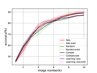
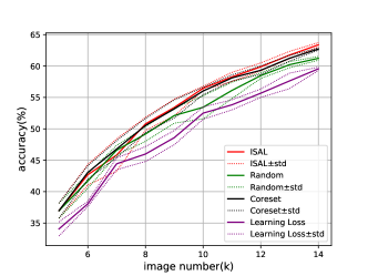
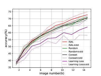
Figure 3: Result for Image Classification. (a) Result on CIFAR10. (b) Result on CIFAR100. (c) Result on SVHN.

4.2 Object Detection

Object detection aims to detect instances of semantic objects of a certain class in images. The detectors are trained to localize the object by drawing bounding boxes(bboxes) and classifying the object inside the bounding box. The bboxes need to be drawn for the specific classes and the category of the object in the bboxes need to be annotated in the active learning task. In practice, we found that the annotation cost of each image differs largely from others. Take COCO dataset as an example, the image in it at most has 63 bboxes and at least has zero bboxes. Thus, the cost of annotating a set of images is highly correlated with the number of bboxes instead of the number of images. Thus, in the following experiments for object detection, we plot the average number of the bounding box and average mAP/AP from three tries.

Datasets. We choose the VOC2012 [6], which has been widely used in other active learning methods for object detection [15, 40], and COCO [20], a dataset that is commonly used to evaluate the performance of a detector. VOC2012 has 5717 images for training and 5823 images for validation, we use the trainset as the unlabeled dataset and use the validation set to evaluate the trained model performance. We use the mAP as the evaluation metric. COCO dataset has 118k images for training and 5000 images for validation. We use the trainset as the unlabeled dataset, and validate the model performance on the validation set. We use AP as the evaluation metric. We use the default data preparation pipeline which includes the random flipping, image normalization with channel mean and standard deviation, image resizing, and padding from the mmdetection [2].

Active Learning Settings. For the experiments on VOC2012, we randomly select 500 images from the unlabeled set as the initial labeled dataset, and in each of the following steps of the active learning cycle, we add the 500 images to the labeled set. We simulate 10 active learning iteration steps. For COCO, we randomly select 5000 images from the unlabeled set first and add 1000 images in the following step. Since the number of bounding boxes selected by different methods has huge differences, for clearer comparison, we continue the active learning iteration until the trained model achieves $22\pm 0.3\%$ in AP.

Target Model. We use FCOS [37] detector with backbone ResNet-50 implemented in mmdetection to verify our method. We also implement the active learning pipeline and different active learning methods base on mmdetection. We train the model for 12 epochs with the mini-batch size of 8 and the initial learning rate of 0.01. After training 8 and 11 epochs, we decrease the learning rate by 0.1 respectively. The momentum and the weight decay are 0.9 and 0.0001 respectively.

Implement Details. For both datasets, when calculating the influence of the unlabeled data, we backpropagate the loss to the parameters in FCOS’s last convolution layer, which contains three kernels used to generate the final prediction of classification, regression, and centerness score. We use the validation set as reference set. When calculating the $s_{test}$, we random sample at most 5000 images from the labeled set. We repeatedly calculate the $s_{test}$ 4 times and use the value after averaging. We compare our method with random sampling, coreset sampling [31], learning loss sampling [40] and localization stability sampling [15].

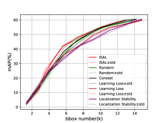
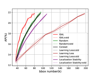
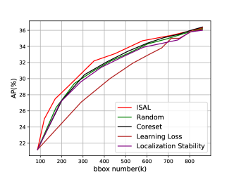
Figure 4: Result for Object Detection. (a) Result on VOC2012. (b) Result on COCO. (c) Result on COCO within a large-scale setting.

Results. The result on VOC2012 and COCO are shown in Figure 4 and Figure 4 respectively. For VOC2012 dataset, when the trained model achieves 42% in mAP, our method uses roughly 850 bboxes fewer than coreset sampling, saving 13% of annotations, and saves roughly 2000 bboxes than localization stability sampling, decreasing the annotations by 26%. Since the VOC2012 only has less than 6000 images, in the last iteration of active learning, different methods have selected similar images. Thus, all methods achieve similar performance. Our method becomes more effective when it is applied to a large dataset.

For COCO, when achieving the target AP, it costs 15.3k fewer bounding boxes than random and 117k fewer bounding boxes than the learning loss sampling, saving 16% and 59% annotation respectively. Our implementations show that all comparing methods perform worse than random sampling, meaning that their reported performance enhancement over random sampling is mainly caused by selecting the image with more bounding boxes. Choose these images significantly enhance the annotation cost, which is contradictory to the purpose of active learning.

4.3 Large Scale Experiment in Object Detection

In this section, we conduct experiments on the large-scale active learning setting for object detection. It aims to prove that our method can be effective when the trained model performance is close to the performance of the model trained on the full dataset. This experiment further validates the superiority of ISAL which can precisely select the samples with the most positive influence on model performance.

Datasets and Experiment Details. We use the COCO trainset as the unlabeled dataset, and validate the trained model performance on the validation set. We plot the number of the bounding boxes and AP to show the model performance. We randomly select 10% images from the unlabeled set first and add the same number of images as the first step in the following steps. We iterate an active learning pipeline 10 times. We continue to use the FCOS detector with backbone ResNet-50 implemented in mmdetection to verify our method. All other experiment details are the same as we described in Section 4.2.

Results. The result is shown in Figure 4. When the trained model performance achieve 34% in AP, which is close to the performance of the FCOS trained on full COCO dataset, our method uses roughly 40k bounding boxes fewer than the coreset sampling, which has the best performance in all comparing methods, decreasing the annotation cost by 8%. This also indicates that achieving 94.4% performance of the model trained on full COCO dataset, we just need 60.7% of the annotations of the dataset.

4.4 Ablation Study

In this section, to validate the effectiveness of UUIC and ISAL, we conduct experiments to discuss the properties of each element in $-\nabla_{\theta}l(R,\hat{\theta})^{T}H_{\hat{\theta}}^{-1}G_{z^{{}^{\prime}}}$. We conduct all the ablation studies on CIFAR10. All the experiment details are the same as mentioned in section 4.1.

4.4.1 The Effect of K in Expected gradient

In this section, we discuss the effect of $K$ in the expected gradient $G_{z^{{}^{\prime}}}$ with which we calculate the influence of the unlabeled sample. Tab. 1 shows the results. When $K$ is equal to 1, our active learning algorithm achieves the best result in each step. Our analysis shows that, in some cases, the direction of the gradient vector computed with the label of the first predicted class is just the opposite of the one computed with the label of the second predicted class. Therefore, when averaging the gradient, some value in the $G_{z^{{}^{\prime}}}$ will be diminished, making the influence of $z^{{}^{\prime}}$ inaccurate.

$K$	number of CIFAR10 images
	1000	3000	5000	7000	9000
1	45.52	67.72	81.24	85.96	89.26
2	45.52	65.65	81.20	85.37	88.15
5	45.52	65.19	78.52	85.43	89.13
10	45.52	62.26	72.28	80.14	83.03

Table 1: The effect of $K$ in $G_{z^{{}^{\prime}}}$.

4.4.2 The Effect of $H_{\hat{\theta}}^{-1}$

In this section, we discuss the effect of $H_{\hat{\theta}}^{-1}$. We compare the performance of ISAL with Gradient Similarity. They use $-\nabla_{\theta}l(R,\hat{\theta})^{T}H_{\hat{\theta}}^{-1}G_{z^{{}^{\prime}}}$ and $-\nabla_{\theta}l(R,\hat{\theta})^{T}G_{z^{{}^{\prime}}}$ to evaluate and select the unlabeled samples, respectively. $-\nabla_{\theta}l(R,\hat{\theta})^{T}G_{z^{{}^{\prime}}}$ measures the similarity of gradients on reference set and the expected gradients of an untrained and unlabeled samples.

Tab. 2 shows that Gradient Similarity has a similar performance as ISAL, though the ISAL performs better. In essence, the Gradient Similarity uses the gradients on the reference set to evaluate which parameters in the model have not been learned well and selects the unlabeled images with a similar expected gradient to train in the next step. This will help the model to obtain the biggest backpropagated gradients on specific model parameters, moving to the global optimal quickly. However, some unlabeled images with different expected gradients also provide a positive influence on the model. A similar phenomenon is mentioned in  [16]. $H_{\hat{\theta}}^{-1}$ helps ISAL to find these samples and enhances ISAL performance.

Method	number of CIFAR10 images
	1000	3000	5000	7000	9000
ISAL	45.52	67.72	81.24	85.96	89.26
Grad Simi	45.52	67.54	80.54	85.72	88.60

Table 2: The effect of $H_{\hat{\theta}}^{-1}$ on the performance of ISAL.

4.4.3 The Selection of Reference Set

In this section, we try different substitutes for using the validation set as the reference set. We try using the $L_{1}$ as the reference set in each step of the iteration, named as ISAL_v2, and using the labeled dataset of each step $L_{i}$ as the reference set, named as ISAL_v3.

Tab. 3 shows that the ISAL_v2 and ISAL_v3 performance is slightly worse than the ISAL, but they still perform much better than random sampling. In essence, the gradients on the reference set represent whether the model parameters have fit in with the data distribution or not. Thus, to ensure that the calculated influence value can precisely represent the model performance change, the distribution of the reference set needs to be similar to the distribution of the $U_{0}$. Since the $L_{1}$ is also randomly sampled from $U_{0}$, the performance of ISAL_v2 is more close to ISAL than ISAL_v3. However, $L_{1}$ has been trained. The model gradients on $L_{1}$ become smaller than the gradients on the validation set, and the calculated influence value may not be precise, explaining why ISAL_v2 performs worse than ISAL.

Method	number of CIFAR10 images
	1000	3000	5000	7000	9000
ISAL	45.52	67.72	81.24	85.96	89.26
ISAL_v2	45.52	67.06	80.57	85.71	88.92
ISAL_v3	45.52	67.12	80.11	84.88	88.71
coreset	45.52	67.66	79.93	85.36	88.61
random	45.52	67.55	77.77	83.09	86.50

Table 3: Comparision of different reference set.

4.5 Visualization Analysis

Figure. 5 shows the tSNE embeddings of the CIFAR10 training set. The red dots represent the images in $S_{1}$ selected by ISAL. Our proposed method tends to choose more images with cat, bird, and deer. Our analysis shows that $M_{1}$ has lower accuracy in these three classes. Thus selecting the images of these three classes can provide a more positive influence on the model performance. In addition, the $M_{1}$ is trained on $L_{1}$ which is randomly sampled, but the model performs worse in these three classes than the other, indicating that these three classes are hard to learn. Thus, evenly sampling images from all classes would lead to data redundancy. Instead, our proposed method selects samples in bias enhancing the learning efficiency.

Figure. 6 shows some selected images of COCO dataset in $S_{1}$ by different methods. Our proposed method selects images with fewer bboxes, while the bboxes’ size in the selected images is significantly larger than the one selected by other methods. In addition, the bboxes in the selected images of our proposed method have a lower overlap ratio. This indicates that the clear and large object in the image helps the model learn more effectively. In the latter of the iteration, our proposed method will select the images with more objects and more complex scenarios, this would help the model to learn from the easy to the difficult step by step.

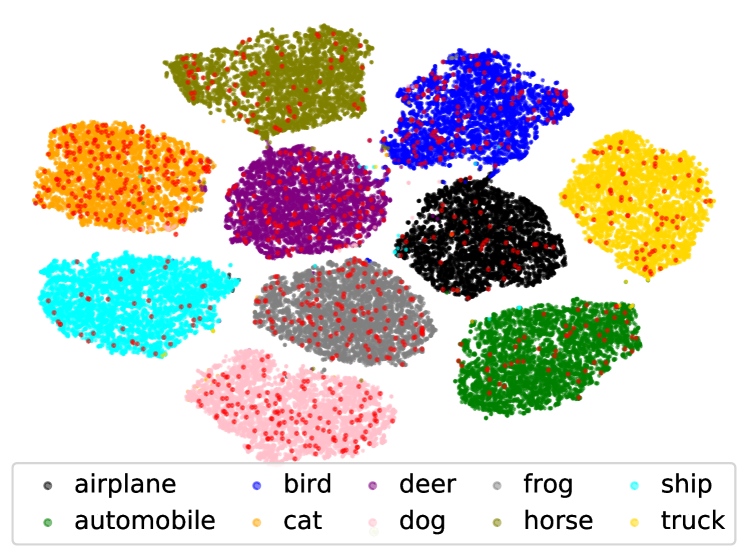
Figure 5: The tSNE embeddings of the CIFAR10 training set. The red dots represent the images in $S_{1}$ selected by ISAL.

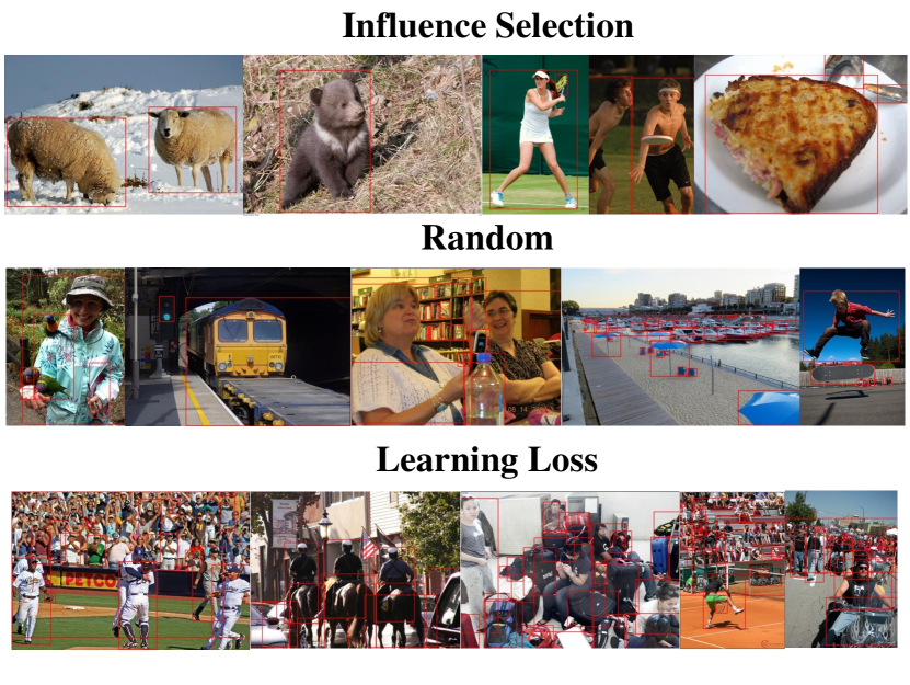
Figure 6: The selected images in COCO dataset by different active learning algorithms.

5 Conclusion

We have proposed a task-agnostic and model-agnostic active learning algorithm, Influence Selection for Active Learning(ISAL), helping neural networks model to learn more effectively and decreasing the annotation cost. By making use of the Untrained Unlabeled sample Influence Calculation(UUIC) to calculate the influence value for each unlabeled sample, ISAL selects the samples which can provide the most positive influence on model performance. ISAL achieves state-of-the-art performance on different tasks in both commonly use settings and a newly-designed large-scale setting. We believe that ISAL can be extended to solve many active learning problems in other areas, and it would not be restricted to the tasks in computer vision.

Acknowledgement: We thank Zheng Zhu for implementing the classification pipeline, Bin Wang and Xizhou Zhu for helping with the experiments, and thank Yuan Tian and Jiamin He for discussing the mathematic derivation.

Supplementary Material

In this supplementary material, we provide additional details which we could not include in the main paper due to space constraints. The material is composed as follows:

1. The derivation of the influence of untrained samples.

2. The implementation details of $s_{test}$ calculation.

3. The time complexity analysis.

4. The implementation details of comparing methods.

5. Additional experiments on CIFAR10 dataset and COCO dataset.

6. The tables in which we report the average performance for each plot.

Appendix A The Derivation of the Influence of Untrained Samples

Newton Step and Quadratic Approximation. Assuming that we have labeled dataset $L_{i}$ and loss function $\mathcal{L}(\theta)=\frac{1}{n}\textstyle\sum_{z\in L_{i}}l(z,\theta)$. After training a model on $L_{i}$, we have the model parameters $\hat{\theta}\in\Theta$, where $\hat{\theta}=\arg\min\;_{\theta\in\Theta}\;\frac{1}{n}\sum_{z\in L_{i}}l(z,\theta)$. Our purpose is to estimate the parameters of model which is trained on $L_{i}$ and the new added sample $z^{{}^{\prime}}$. The new loss function is $\mathcal{L}_{z^{{}^{\prime}}}(\theta)=\frac{1}{n+1}\textstyle\sum_{z^{{}^{\prime}}\cup L_{i}}l(z,\theta)$, giving new trained model parameter $\hat{\theta}_{z^{{}^{\prime}}}=\arg\min\;_{\theta\in\Theta}\;\frac{1}{n+1}\textstyle\sum_{z^{{}^{\prime}}\cup L_{i}}l(z,\theta)$.

Considering the quadratic approximation of the $\mathcal{L}_{z^{{}^{\prime}}}(\hat{\theta}_{z^{{}^{\prime}}})$

$$\mathcal{L}_{z^{{}^{\prime}}}(\hat{\theta}_{z^{{}^{\prime}}})=\mathcal{L}_{z^{{}^{\prime}}}(\hat{\theta})+(\hat{\theta}_{z^{{}^{\prime}}}-\hat{\theta})^{T}\nabla_{\theta}\mathcal{L}_{z^{{}^{\prime}}}(\hat{\theta})+$$ (5)

$$\frac{1}{2}(\hat{\theta}_{z^{{}^{\prime}}}-\hat{\theta})^{T}\nabla_{\theta}^{2}\mathcal{L}_{z^{{}^{\prime}}}(\hat{\theta})(\hat{\theta}_{z^{{}^{\prime}}}-\hat{\theta})$$

If the $H_{\hat{\theta}}^{-1}$ is positive definite, the quadratic approximation is minimized at

$$\hat{\theta}_{z^{{}^{\prime}}}-\hat{\theta} =-\frac{\nabla_{\theta}\mathcal{L}_{z^{{}^{\prime}}}(\hat{\theta})}{\nabla_{\theta}^{2}\mathcal{L}_{z^{{}^{\prime}}}(\hat{\theta})}$$ (6)

$$=-[\nabla_{\theta}^{2}\mathcal{L}_{z^{{}^{\prime}}}(\hat{\theta})]^{-1}[\nabla_{\theta}\mathcal{L}_{z^{{}^{\prime}}}(\hat{\theta})]$$

Thus, the quadratic approximation of $\hat{\theta}_{z^{{}^{\prime}}}$ is equal to $\hat{\theta}-[\nabla_{\theta}^{2}\mathcal{L}_{z^{{}^{\prime}}}(\hat{\theta})]^{-1}[\nabla_{\theta}\mathcal{L}_{z^{{}^{\prime}}}(\hat{\theta})]$, and $-[\nabla_{\theta}^{2}\mathcal{L}_{z^{{}^{\prime}}}(\hat{\theta})]^{-1}[\nabla_{\theta}\mathcal{L}_{z^{{}^{\prime}}}(\hat{\theta})]$ is the newton step.

Evaluate the Influence of an Untrained Sample. First we add a small influence from $z^{{}^{\prime}}$ to the loss function $\mathcal{L}(\theta)$, the new loss function is

$$\mathcal{L}_{\varepsilon,z^{{}^{\prime}}}(\theta) =\arg\min\;_{\theta\in\Theta}\;\frac{1}{n}\sum_{z\in L_{i}}l(z,\theta)+\varepsilon l(z^{{}^{\prime}},\theta)$$ (7)

$$=\mathcal{L}(\theta)+\varepsilon l(z^{{}^{\prime}},\theta)$$

With new loss function, the model new parameters is obtained $\hat{\theta}_{\varepsilon,z^{{}^{\prime}}}=\arg\min\;_{\theta\in\Theta}\;\mathcal{L}_{\varepsilon,z^{{}^{\prime}}}(\theta)$. We evaluate a sample $z^{{}^{\prime}}$ importance by calculating the ${\left.\frac{\displaystyle\operatorname{d}\hat{\theta}_{\varepsilon,z^{{}^{\prime}}}}{\displaystyle\operatorname{d}\varepsilon}\right|}_{\varepsilon=0}$

From equation 6 we know that

$$\hat{\theta}_{\varepsilon,z^{{}^{\prime}}}-\hat{\theta}= -[\nabla_{\theta}^{2}\mathcal{L}_{\varepsilon,z^{{}^{\prime}}}(\hat{\theta})]^{-1}[\nabla_{\theta}\mathcal{L}_{\varepsilon,z^{{}^{\prime}}}(\hat{\theta})]$$ (8)

$$= -[\nabla_{\theta}^{2}\mathcal{L}(\hat{\theta})+\varepsilon\nabla_{\theta}^{2}l(z^{{}^{\prime}},\hat{\theta})]^{-1}$$

$$\qquad[\nabla_{\theta}\mathcal{L}(\hat{\theta})+\varepsilon\nabla_{\theta}l(z^{{}^{\prime}},\hat{\theta})]$$

Since $\hat{\theta}$ minimizes $\mathcal{L}(\theta)$, $\nabla_{\theta}\mathcal{L}(\hat{\theta})$ is equal to 0. Dropping the $O(\varepsilon^{2})$ terms, we have

$$\hat{\theta}_{\varepsilon,z^{{}^{\prime}}}-\hat{\theta}\approx-[\nabla_{\theta}^{2}\mathcal{L}(\hat{\theta})]^{-1}\varepsilon\nabla_{\theta}l(z^{{}^{\prime}},\hat{\theta})$$ (9)

We define $H_{\hat{\theta}}^{-1}\overset{def}{=}[\nabla_{\theta}^{2}\mathcal{L}(\hat{\theta})]^{-1}$, and we have

$$\hat{\theta}_{\varepsilon,z^{{}^{\prime}}}-\hat{\theta}\approx-H_{\hat{\theta}}^{-1}\varepsilon\nabla_{\theta}l(z^{{}^{\prime}},\hat{\theta})$$ (10)

Thus, we can evaluate a untrained sample by:

$${\left.\frac{\displaystyle\operatorname{d}\hat{\theta}_{\varepsilon,z^{{}^{\prime}}}}{\displaystyle\operatorname{d}\varepsilon}\right|}_{\varepsilon=0} ={\left.\frac{\hat{\theta}_{\varepsilon,z^{{}^{\prime}}}-\hat{\theta}}{\displaystyle\operatorname{\varepsilon}}\right|}_{\varepsilon=0}$$ (11)

$$={\left.\frac{-\varepsilon H_{\hat{\theta}}^{-1}\nabla_{\theta}l(z^{{}^{\prime}},\hat{\theta})}{\displaystyle\operatorname{\varepsilon}}\right|}_{\varepsilon=0}$$

$$=-H_{\hat{\theta}}^{-1}\nabla_{\theta}l(z^{{}^{\prime}},\hat{\theta})$$

Appendix B The Implementation Details of $s_{test}$ Calculation

To evaluate an untrained unlabeled sample, $I(z^{{}^{\prime}},R)=-\nabla_{\theta}l(R,\hat{\theta})^{T}H_{\hat{\theta}}^{-1}G_{z^{{}^{\prime}}}$ needs to be calculated. However, it’s impossible to calculate the inverse matrix of the Hessian matrix due to the memory constrain of GPU and the time complexity, especially for the deep neural network. We use the method proposed by Agarwal [1] to effectively approximate the $s_{test}\overset{def}{=}H_{\hat{\theta}}^{-1}\nabla_{\theta}l(R,\hat{\theta})$ and then calculate $I(z^{{}^{\prime}},R)=-s_{test}\cdot G_{z^{{}^{\prime}}}$ for each samples.

Dropping the $\hat{\theta}$ subscript for clarity, we define

$$H_{j}^{-1}\overset{def}{=}\textstyle\sum_{i=0}^{j}(I-H)^{i}$$ (12)

as the first j terms in the Taylor expansion of $H^{-1}$. When $j\rightarrow\infty$, we have $H_{j}^{-1}\rightarrow H^{-1}$.

From equation 12, we have

$$H_{j}^{-1}=I+(I-H)H_{j-1}^{-1}$$ (13)

The key idea of stochastic estimation is that we can substitute the full $H$ in equation 13 with the any unbiased estimator of $H$ to form $\tilde{H}_{j}$. Since $\mathbb{E}[\tilde{H}_{j}^{-1}]=H_{j}^{-1}$, we still have $\mathbb{E}[\tilde{H}_{j}^{-1}]=H^{-1}$, when $j\rightarrow\infty$. In practice, we can randomly sample $z_{i}$ and use $\nabla_{\theta}^{2}l(z_{i},\hat{\theta})$ as the unbiased estimator of $H$. Algorithm 3 shows how we approximate the $s_{test}$.

Algorithm 3 The calculation of $s_{test}$

1:Input: $v=\nabla_{\theta}l(R,\hat{\theta})$

2:Random sample $k$ images $\{z_{1},z_{2},\cdots,z_{k}\}$ from labeled dataset

3:initial the $s_{test_{0}}=v$

4:for $i$ in range($1$, $k+1$) do

5:    $s_{test_{i}}=v+(I-\nabla_{\theta}^{2}l(z_{i},\hat{\theta}))s_{test_{i-1}}$

6:end for

7:take the $s_{test_{k}}$ as the unbiased estimator of $s_{test}$

8:Return $s_{test}$

In practice, we calculate the Hessian-vector products of $\nabla_{\theta}^{2}l(z_{i},\hat{\theta})s_{test_{i-1}}$ instead of calculating the Hessian matrix $\nabla_{\theta}^{2}l(z_{i},\hat{\theta})$. We will repeat the algorithm 3 $p$ times, and use the averaged result as the final estimation of $s_{test}$.

Appendix C The Time Complexity Analysis

As demonstrated in Section B, our method can be divided into two sections. First, instead of directly calculate the $H_{\hat{\theta}}^{-1}$, we sample images from the labeled dataset to calculate the $s_{test}$, which is the stochastic estimation of $\nabla_{\theta}l(R,\hat{\theta})^{T}H_{\hat{\theta}}^{-1}$. Since the number of sampled images is fixed, the time complexity is a constant $C$. Then, we calculate the influence for each unlabeled sample with $s_{test}$. Noted that $|U|=n$, the time complexity is $O(n)$.

Appendix D The Implementation Details of Comparing Methods

D.1 Image Classification

For coreset sampling [31], we follow [40] and implement the K-Ceter-Greedy algorithm, which is just slightly worse than the mixed-integer program but much less time-consuming. We run the algorithm by using the feature before the classification layer as [31] reported. For the learning loss sampling, we connect the learning loss module to each block of ResNet-18, stopping the loss prediction module gradient from back-propagating to the model after 120 epochs, and set the $\lambda$ to 1 as [40] do. We first randomly select a subset with 10000 images from unlabeled samples before predicting the loss and selecting the image with the largest predicted loss.

D.2 Object Detection

For coreset sampling, we implement the K-Ceter-Greedy algorithm. We apply global average pooling on the feature after the regression branch and the classification branch of FCOS [37], then we concatenate the features from both branches and use this to run the algorithm. We also tried using the feature from the Feature Pyramid Network(FPN) of FCOS to run the algorithm, but it does not perform better.

For the learning loss sampling, we use the 5 feature maps from the FPN of FCOS. We stopping the loss of the loss prediction module from back-propagating to the backbone, otherwise, the detector performance would deteriorate significantly. We set the $\lambda$ to 1.

For localization stability sampling [15], we implement the Localization Stability method in the paper, since its performance is evaluated on both VOC2012 [6] and COCO [20] datasets.

D.3 Large Scale Experiment in Object Detection

All the implementation details of the comparing methods are exactly the same as D.2

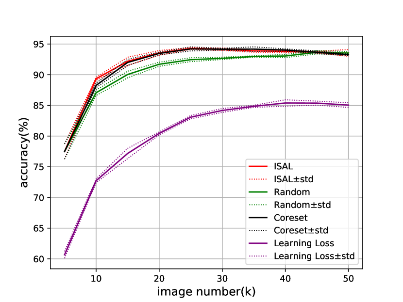
Figure 7: Result for CIFAR10 in large-scale active learning setting.

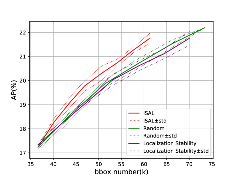
Figure 8: Result for COCO with Faster R-CNN.

Appendix E Additional Experiments

E.1 Image Classification

In this section, we provide additional experiments on image classification with CIFAR10 in large scale active learning setting.

Active Learning Settings. For the experiments on CIFAR10, we randomly select 5000 images from the unlabeled set as the initial labeled dataset, and in each of the following steps, we add 5000 images to the labeled dataset. The simulate 10 active learning steps and stop the active learning iteration. All other implementation details are exactly the same as we described in the main paper.

Results. The results on CIFAR10 with large-scale active learning setting are shown in Figure 7. Our proposed method outperforms all comparing methods before step 6. Our implementation shows that both our method and coreset sampling achieve the best performance at step 5, and the performance of the trained model deteriorates when we keep enlarging the labeled dataset. In practice, it is not necessary to continue the active learning iteration after step 5. This phenomenon indicates that, when using the ResNet-18 as the classifier and using the test set of CIFAR10 as the benchmark to evaluate the model performance, some images in the training set of CIFAR10 provide a negative influence on the model’s performance. Active learning algorithm does help trained model to achieve better performance with fewer annotations.

E.2 Object Detection

In this section, we provide additional experiments on object detection with the COCO dataset.

Active Learning Settings. We randomly select 5000 images from the unlabeled set first and add 1000 images in the following steps. Since the number of bounding boxes selected by different methods has huge differences, for clearer comparison, we continue the active learning iteration until the trained model achieves $22\pm 0.3\%$ in AP.

Target Model. We use Faster R-CNN [27] detector with backbone ResNet-50 implemented in mmdetection [2] to verify our method. We train the model for 12 epochs with the mini-batch size of 8 and the initial learning rate of 0.01. After training 8 and 11 epochs, we decrease the learning rate by 0.1 respectively. The momentum and the weight decay are 0.9 and 0.0001 respectively.

Implementation Details. When calculating the influence of the unlabeled data, we backpropagate the loss to the parameters in the last convolution layer for regression and classification in Region Proposal Network(RPN), and to fully connected layer for regression result and classification result in Region of Interest Network(RoI) of Faster R-CNN. We use the validation set as reference set. When calculating the $s_{test}$, we random sample at most 500 images from the labeled set. We repeatedly calculate the $s_{test}$ 4 times and use the value after averaging. We compare our method with random sampling and localization stability sampling [15], which can be implemented in Faster R-CNN easily. For localization stability sampling [15], we implement the Localization Stability method in the paper.

Results. The results on Faster R-CNN are shown in Figure 8. When achieving $21.8$ in AP, our method cost 7.1k fewer bounding boxes than random sampling, saving 10.4% annotations. This result shows that our method can be effective in both one-stage and two-stage detectors. It further substantiates that our method is task-agnostic and model-agnostic.

Appendix F The Experiment Results

Table 4, table 5 and table 6 show the experiment results on the image classification of the main paper. Table 7 shows the experiment result of Section E.1 in supplementary material.

Table 8, table 9 and table 10 show the experiment results on the object detection of the main paper. Table 11 shows the experiment result of Section E.2 in supplementary material.

Methods	5 times average of Accuracy(%) in each step
	1	2	3	4	5
ISAL	45.51799931	54.86599902	67.72399840	76.69599825	81.23799817
coreset	45.51799931	58.29599852	67.65599847	75.99799808	79.93399816
random	45.51799931	58.40199852	67.44199847	72.30399829	77.86199819
learningloss	45.91599973	58.88999852	69.14799823	75.80599807	80.11599825
Methods	5 times average of Accuracy(%) in each step
	6	7	8	9	10
ISAL	83.61199812	85.95799826	88.05599827	89.26399810	89.95799797
coreset	81.53599801	85.36399841	87.19999817	88.61399807	89.05199809
random	81.93599806	83.05799810	84.75199825	86.45999833	87.28999833
learningloss	82.25999810	84.46999836	85.10199790	86.66799833	87.07999842

Table 4: The experiment results on CIFAR10 with ResNet-18.

Methods	5 times average of Accuracy(%) in each step
	1	2	3	4	5
ISAL	36.97799921	42.69599870	45.82199922	50.78799950	53.40799696
coreset	36.97799921	43.06599873	46.78799956	50.53399960	53.17999910
random	36.97799921	41.70599863	46.59999991	49.17400009	52.11799930
learningloss	34.06799937	38.06399904	44.43599916	45.98999956	48.60199980
Methods	5 times average of Accuracy(%) in each step
	6	7	8	9	10
ISAL	56.45799872	58.26799854	59.87199865	61.7459986	63.37799866
coreset	56.02399869	58.10799861	59.32599477	61.24399836	62.70399857
random	53.43599904	56.11799880	58.47799854	60.21399841	61.22999834
learningloss	52.50199925	53.82599889	55.67399864	57.63399866	59.55999863

Table 5: The experiment results on CIFAR100 with ResNet-18.

Methods	5 times average of Accuracy(%) in each step
	1	2	3	4	5
ISAL	37.82575205	47.63829102	54.23709167	57.31100053	61.49200840
coreset	37.82575205	48.01090959	53.73232837	57.43315776	60.21665482
random	37.82575205	48.01090931	52.56760825	57.24646455	60.07759528
learningloss	38.82068125	43.61785414	50.38337374	52.06561057	55.83128330
Methods	5 times average of Accuracy(%) in each step
	6	7	8	9	10
ISAL	65.13214355	66.81315140	69.44836955	71.31146101	72.86339711
coreset	62.84495852	65.01152269	66.76705426	68.27980783	70.82436816
random	62.97172561	65.16671630	65.52473728	69.23401795	70.40181142
learningloss	56.31453489	59.98309629	58.65165838	61.91687003	64.04348344

Table 6: The experiment results on SVHN with ResNet-18.

Methods	5 times average of Accuracy(%) in each step
	1	2	3	4	5
ISAL	77.48999786	89.33399824	92.19199778	93.55399844	94.27999855
coreset	77.48999786	88.25799831	92.00199783	93.46399852	94.20599862
random	77.48999786	87.05999821	90.03599803	91.70399761	92.44999793
learningloss	60.66199856	72.72399856	77.17199846	80.43999806	83.08399811
Methods	5 times average of Accuracy(%) in each step
	6	7	8	9	10
ISAL	94.15999845	93.89199833	93.80199861	93.68999855	93.54599838
coreset	94.15399850	94.16999856	94.02599862	93.66199836	93.24799830
random	92.66799801	92.97199826	93.04599803	93.65399836	93.53199820
learningloss	84.17599796	84.85199794	85.39199788	85.36999783	85.04999776

Table 7: The experiment results on CIFAR10 in large-scale setting with ResNet-18.

Method		3 times average of results in each step
		1	2	3	4	5
ISAL	mAP	0.02366667	0.12766667	0.24633333	0.32366667	0.42
	bbox num	1338	2777.66667	3606.66667	4446	5616
	10k $\times$ mAP / bbox num	0.17688092	0.45961839	0.68299445	0.72799520	0.74786325
Coreset	mAP	0.02366667	0.13	0.25733333	0.38466667	0.459
	bbox num	1338	2624.66667	4149.33333	5736.66667	7292.66667
	10k $\times$ mAP / bbox num	0.17688092	0.49530099	0.62017995	0.67054038	0.62939940
Random	mAP	0.02366667	0.11666667	0.24133333	0.342	0.43666667
	bbox num	1338	2683.66667	4097.66667	5450.66667	6833.66667
	10k $\times$ mAP / bbox num	0.17688092	0.43472861	0.58895306	0.62744618	0.63899322
Learningloss	mAP	0.023	0.13	0.25233333	0.35933333	0.42433333
	bbox num	1338	2780.66667	4161.66667	5627	7236
	10k $\times$ mAP / bbox num	0.17189836	0.46751379	0.60632759	0.63858776	0.58641975
Localization stability	mAP	0.02366667	0.136	0.243	0.33233333	0.4245
	bbox num	1338	2713.33333	3940.66667	5653	7601.66667
	10k $\times$ mAP / bbox num	0.17688092	0.50122850	0.61664693	0.58788844	0.55843017
Method		3 times average of results in each step
		6	7	8	9	10
ISAL	mAP	0.47166667	0.515	0.55233333	0.57666667	0.596
	bbox num	7190.33333	8703.66667	10160	11503	12967.6667
	10k $\times$ mAP / bbox num	0.65597330	0.59170465	0.54363517	0.50131850	0.45960466
Coreset	mAP	0.51033333	0.552	0.57666667	0.59666667	0.604
	bbox num	8812	10286.3333	11635	12888.3333	14194.3333
	10k $\times$ mAP / bbox num	0.57913451	0.53663437	0.49563100	0.46295099	0.42552192
Random	mAP	0.4845	0.53533333	0.56133333	0.57866667	0.595
	bbox num	8188.33333	9575.66667	11011.6667	12426	13813
	10k $\times$ mAP / bbox num	0.59169550	0.55905594	0.50976237	0.46569022	0.43075364
Learningloss	mAP	0.49566667	0.54866667	0.566	0.58266667	0.59866667
	bbox num	8752.33333	10368	11750	12981.6667	14119.3333
	10k $\times$ mAP / bbox num	0.56632517	0.52919239	0.48170213	0.44883811	0.42400491
Localization stability	mAP	0.46533333	0.52766667	0.55933333	0.59	0.60466667
	bbox num	9169.66667	11056.3333	12580	13853.6667	14843.6667
	10k $\times$ mAP / bbox num	0.50747028	0.47725286	0.44462109	0.42588003	0.40735667

Table 8: The experiment results on VOC2012 with FCOS.

Method		3 times average of results in each step
		1	2	3	4	5
ISAL	AP	0.12833333	0.14433333	0.153	0.16233333	0.166
	bbox num	36603.6667	37934	40028.3333	42021	43947.3333
	10k $\times$ AP / bbox num	0.03506024	0.03804854	0.03822293	0.03863148	0.03777249
Coreset	AP	0.12833333	0.15266667	0.17333333	0.18766667	0.19833333
	bbox num	36603.6667	47194	57032.3333	66384.3333	75564.3333
	10k $\times$ AP / bbox num	0.03506024	0.03234875	0.03039212	0.02826972	0.02624695
Random	AP	0.12833333	0.15033333	0.16566667	0.17733333	0.188
	bbox num	36603.6667	44055.6667	51381.3333	58653.6667	66240
	10k $\times$ AP / bbox num	0.03506024	0.03412350	0.03224258	0.03023397	0.02838164
Learningloss	AP	0.127	0.147	0.163	0.17766667	0.185
	bbox num	36603.6667	62127.6667	84566.3333	105900.333	126722.333
	10k $\times$ AP / bbox num	0.03469598	0.02366096	0.01927481	0.01677678	0.01459885
Localization stability	AP	0.12833333	0.149	0.16566667	0.179	0.191
	bbox num	36603.6667	47503.3333	58252.6667	69085.6667	79574.6667
	10k $\times$ AP / bbox num	0.03506024	0.03136622	0.02843933	0.02590986	0.02400261
Method		3 times average of results in each step
		6	7	8	9	10
ISAL	AP	0.172	0.18666667	0.18333333	0.189	0.19133333
	bbox num	45810	47864.6667	49865	51930.6667	54414.3333
	10k $\times$ AP / bbox num	0.03754639	0.03899884	0.03676594	0.03639468	0.03516230
Coreset	AP	0.20933333	0.21766667	N/A	N/A	N/A
	bbox num	84924	94075.6667	N/A	N/A	N/A
	10k $\times$ AP / bbox num	0.02464949	0.02313740	N/A	N/A	N/A
Random	AP	0.199	0.20533333	0.21433333	0.22	N/A
	bbox num	73457	80720.6667	88030.6667	95464.3333	N/A
	10k $\times$ AP / bbox num	0.02709068	0.02543752	0.02434758	0.02304526	N/A
Learningloss	AP	0.19433333	0.20233333	0.21166667	0.21766667	N/A
	bbox num	145197	163798	181040.333	197804	N/A
	10k $\times$ AP / bbox num	0.01338412	0.01235261	0.01169169	0.01100416	N/A
Localization stability	AP	0.2	0.20866667	0.217	N/A	N/A
	bbox num	89557.3333	99480.6667	109179.333	N/A	N/A
	10k $\times$ AP / bbox num	0.02233206	0.0209756	0.01987556	N/A	N/A
Method		3 times average of results in each step
		11	12	13	14	15
ISAL	AP	0.19466667	0.197	0.20233333	0.207	0.20933333
	bbox num	56457	59059	61677	64093.3333	66729
	10k $\times$ AP / bbox num	0.03448052	0.03335647	0.03280531	0.03229665	0.03137067
Method		3 times average of results in each step
		16	17	18	19	20
ISAL	AP	0.21	0.21133333	0.216	0.21633333	0.218
	bbox num	69402	72282.3333	74690	77545.6667	80139
	10k $\times$ AP / bbox num	0.03025849	0.02923720	0.02891953	0.0278975	0.02720274

Table 9: The experiment results on COCO with FCOS.

Method		Results in each step
		1	2	3	4	5
ISAL	AP	0.212	0.25	0.275	0.291	0.305
	bbox num	86838	118762	169688	232923	286589
	10k $\times$ AP / bbox num	0.02441328	0.02105050	0.01620621	0.01249340	0.01064242
Coreset	AP	0.212	0.273	0.305	0.321	0.334
	bbox num	86838	201072	307552	413095	510927
	10k $\times$ AP / bbox num	0.02441328	0.01357723	0.00991702	0.00777061	0.00653714
Random	AP	0.212	0.264	0.294	0.309	0.322
	bbox num	86838	173507	259539	345013	430922
	10k $\times$ AP / bbox num	0.02441328	0.01521552	0.01132778	0.00895618	0.00747235
Learningloss	AP	0.212	0.271	0.3	0.319	0.33
	bbox num	86838	291934	426039	532231	609475
	10k $\times$ AP / bbox num	0.02441328	0.00928292	0.00704161	0.00599364	0.00541450
Localization stability	AP	0.212	0.271	0.296	0.314	0.327
	bbox num	86838	194677	289580	385590	485663
	10k $\times$ AP / bbox num	0.02441328	0.01392049	0.0102217	0.00814337	0.00673306
Method		Results in each step
		6	7	8	9	10
ISAL	AP	0.322	0.331	0.347	0.354	0.363
	bbox num	351747	449780	579039	719234	860001
	10k $\times$ AP / bbox num	0.00915431	0.00735915	0.00599269	0.00492190	0.00422093
Coreset	AP	0.344	0.351	0.355	0.36	0.364
	bbox num	601362	680853	748513	806205	860001
	10k $\times$ AP / bbox num	0.00572035	0.00515530	0.00474274	0.00446537	0.00423255
Random	AP	0.332	0.343	0.349	0.356	0.362
	bbox num	516689	602084	688451	774142	860001
	10k $\times$ AP / bbox num	0.00642553	0.0056969	0.00506935	0.0045986	0.00420930
Learningloss	AP	0.338	0.35	0.35	0.358	0.361
	bbox num	668558	713657	751218	805063	860001
	10k $\times$ AP / bbox num	0.00505566	0.00490432	0.0046591	0.00444686	0.00419767
Localization stability	AP	0.339	0.344	0.348	0.358	0.36
	bbox num	583831	674087	744716	801876	860001
	10k $\times$ AP / bbox num	0.00580648	0.00510320	0.00467292	0.00446453	0.00418604

Table 10: The experiment results on COCO in large-scale setting with FCOS.

Method		3 times average of results in each step
		1	2	3	4	5
ISAL	AP	0.17233333	0.18266667	0.19066667	0.19766667	0.203
	bbox num	36603.6667	40120.3333	43547.3333	46840.6667	50633.3333
	10k $\times$ AP / bbox num	0.04708089	0.04552970	0.04378378	0.04219980	0.04009217
Random	AP	0.17233333	0.18633333	0.19866667	0.207	0.21533333
	bbox num	36603.6667	44055.6667	51381.3333	58653.6667	66240
	10k $\times$ AP / bbox num	0.04708089	0.04229498	0.03866514	0.03529191	0.03250805
Localization stability	AP	0.17333333	0.18266667	0.19133333	0.20033333	0.20633333
	bbox num	36603.6667	42171	47576.3333	53144.6667	59066.3333
	10k $\times$ AP / bbox num	0.04735410	0.04331571	0.04021607	0.03769585	0.03493248
Method		3 times average of results in each step
		1	2	3	4	5
ISAL	AP	0.20733333	0.21266667	0.21766667	N/A	N/A
	bbox num	54060.3333	57655	61360.3333	N/A	N/A
	10k $\times$ AP / bbox num	0.03835221	0.03688608	0.03547351	N/A	N/A
Random	AP	0.222	N/A	N/A	N/A	N/A
	bbox num	73457	N/A	N/A	N/A	N/A
	10k $\times$ AP / bbox num	0.03022176	N/A	N/A	N/A	N/A
Localization stability	AP	0.21133333	0.21766667	N/A	N/A	N/A
	bbox num	64631.3333	70119.3333	N/A	N/A	N/A
	10k $\times$ AP / bbox num	0.03269828	0.03104232	N/A	N/A	N/A

Table 11: The experiment results on COCO with Faster R-CNN.

References

- [1] Naman Agarwal, Brian Bullins, and Elad Hazan. Second-order stochastic optimization in linear time. stat, 1050:15, 2016.
- [2] Kai Chen, Jiaqi Wang, Jiangmiao Pang, Yuhang Cao, Yu Xiong, Xiaoxiao Li, Shuyang Sun, Wansen Feng, Ziwei Liu, Jiarui Xu, et al. Mmdetection: Open mmlab detection toolbox and benchmark. arXiv preprint arXiv:1906.07155, 2019.
- [3] R Dennis Cook and Sanford Weisberg. Residuals and influence in regression. New York: Chapman and Hall, 1982.
- [4] Sai Vikas Desai and Vineeth N Balasubramanian. Towards fine-grained sampling for active learning in object detection. In Proceedings of the IEEE/CVF Conference on Computer Vision and Pattern Recognition Workshops, pages 924--925, 2020.
- [5] Ehsan Elhamifar, Guillermo Sapiro, Allen Yang, and S Shankar Sasrty. A convex optimization framework for active learning. In Proceedings of the IEEE International Conference on Computer Vision, pages 209--216, 2013.
- [6] M. Everingham, L. Van Gool, C. K. I. Williams, J. Winn, and A. Zisserman. The PASCAL Visual Object Classes Challenge 2012 (VOC2012) Results. http://www.pascal-network.org/challenges/VOC/voc2012/workshop/index.html.
- [7] Alexander Freytag, Erik Rodner, and Joachim Denzler. Selecting influential examples: Active learning with expected model output changes. In European Conference on Computer Vision, pages 562--577. Springer, 2014.
- [8] Yarin Gal and Zoubin Ghahramani. Dropout as a bayesian approximation: Representing model uncertainty in deep learning. In international conference on machine learning, pages 1050--1059. PMLR, 2016.
- [9] Yuhong Guo. Active instance sampling via matrix partition. In NIPS, pages 802--810, 2010.
- [10] Mahmudul Hasan and Amit K Roy-Chowdhury. Context aware active learning of activity recognition models. In Proceedings of the IEEE International Conference on Computer Vision, pages 4543--4551, 2015.
- [11] Elmar Haussmann, Michele Fenzi, Kashyap Chitta, Jan Ivanecky, Hanson Xu, Donna Roy, Akshita Mittel, Nicolas Koumchatzky, Clement Farabet, and Jose M Alvarez. Scalable active learning for object detection. In 2020 IEEE Intelligent Vehicles Symposium (IV), pages 1430--1435. IEEE, 2020.
- [12] Kaiming He, Xiangyu Zhang, Shaoqing Ren, and Jian Sun. Deep residual learning for image recognition. In Proceedings of the IEEE conference on computer vision and pattern recognition, pages 770--778, 2016.
- [13] Matthias Hein, Maksym Andriushchenko, and Julian Bitterwolf. Why relu networks yield high-confidence predictions far away from the training data and how to mitigate the problem. In Proceedings of the IEEE/CVF Conference on Computer Vision and Pattern Recognition, pages 41--50, 2019.
- [14] Ajay J Joshi, Fatih Porikli, and Nikolaos Papanikolopoulos. Multi-class active learning for image classification. In 2009 IEEE Conference on Computer Vision and Pattern Recognition, pages 2372--2379. IEEE, 2009.
- [15] Chieh-Chi Kao, Teng-Yok Lee, Pradeep Sen, and Ming-Yu Liu. Localization-aware active learning for object detection. In Asian Conference on Computer Vision, pages 506--522. Springer, 2018.
- [16] Pang Wei Koh and Percy Liang. Understanding black-box predictions via influence functions. In International Conference on Machine Learning, pages 1885--1894. PMLR, 2017.
- [17] Alex Krizhevsky, Geoffrey Hinton, et al. Learning multiple layers of features from tiny images. 2009.
- [18] David D Lewis and Jason Catlett. Heterogeneous uncertainty sampling for supervised learning. In Machine learning proceedings 1994, pages 148--156. Elsevier, 1994.
- [19] David D Lewis and William A Gale. A sequential algorithm for training text classifiers. In SIGIR’94, pages 3--12. Springer, 1994.
- [20] Tsung-Yi Lin, Michael Maire, Serge Belongie, James Hays, Pietro Perona, Deva Ramanan, Piotr Dollár, and C Lawrence Zitnick. Microsoft coco: Common objects in context. In European conference on computer vision, pages 740--755. Springer, 2014.
- [21] Wei Liu, Dragomir Anguelov, Dumitru Erhan, Christian Szegedy, Scott Reed, Cheng-Yang Fu, and Alexander C Berg. Ssd: Single shot multibox detector. In European conference on computer vision, pages 21--37. Springer, 2016.
- [22] Wenjie Luo, Alex Schwing, and Raquel Urtasun. Latent structured active learning. Advances in Neural Information Processing Systems, 26:728--736, 2013.
- [23] Oisin Mac Aodha, Neill DF Campbell, Jan Kautz, and Gabriel J Brostow. Hierarchical subquery evaluation for active learning on a graph. In Proceedings of the IEEE conference on computer vision and pattern recognition, pages 564--571, 2014.
- [24] Hieu T Nguyen and Arnold Smeulders. Active learning using pre-clustering. In Proceedings of the twenty-first international conference on Machine learning, page 79, 2004.
- [25] Ilija Radosavovic, Justin Johnson, Saining Xie, Wan-Yen Lo, and Piotr Dollár. On network design spaces for visual recognition. In ICCV, 2019.
- [26] Pengzhen Ren, Yun Xiao, Xiaojun Chang, Po-Yao Huang, Zhihui Li, Xiaojiang Chen, and Xin Wang. A survey of deep active learning. arXiv preprint arXiv:2009.00236, 2020.
- [27] Shaoqing Ren, Kaiming He, Ross Girshick, and Jian Sun. Faster r-cnn: Towards real-time object detection with region proposal networks. arXiv preprint arXiv:1506.01497, 2015.
- [28] Zhongzheng Ren, Raymond A Yeh, and Alexander G Schwing. Not all unlabeled data are equal: learning to weight data in semi-supervised learning. arXiv preprint arXiv:2007.01293, 2020.
- [29] Dan Roth and Kevin Small. Margin-based active learning for structured output spaces. In European Conference on Machine Learning, pages 413--424. Springer, 2006.
- [30] Soumya Roy, Asim Unmesh, and Vinay P Namboodiri. Deep active learning for object detection. In BMVC, page 91, 2018.
- [31] Ozan Sener and Silvio Savarese. Active learning for convolutional neural networks: A core-set approach. arXiv preprint arXiv:1708.00489, 2017.
- [32] Burr Settles. Active learning. Synthesis lectures on artificial intelligence and machine learning, 6(1):1--114, 2012.
- [33] Burr Settles and Mark Craven. An analysis of active learning strategies for sequence labeling tasks. In Proceedings of the 2008 Conference on Empirical Methods in Natural Language Processing, pages 1070--1079, 2008.
- [34] H Sebastian Seung, Manfred Opper, and Haim Sompolinsky. Query by committee. In Proceedings of the fifth annual workshop on Computational learning theory, pages 287--294, 1992.
- [35] Shuai Shao, Zeming Li, Tianyuan Zhang, Chao Peng, Gang Yu, Xiangyu Zhang, Jing Li, and Jian Sun. Objects365: A large-scale, high-quality dataset for object detection. In Proceedings of the IEEE/CVF International Conference on Computer Vision, pages 8430--8439, 2019.
- [36] Samarth Sinha, Sayna Ebrahimi, and Trevor Darrell. Variational adversarial active learning. In Proceedings of the IEEE/CVF International Conference on Computer Vision, pages 5972--5981, 2019.
- [37] Zhi Tian, Chunhua Shen, Hao Chen, and Tong He. Fcos: Fully convolutional one-stage object detection. In Proceedings of the IEEE/CVF International Conference on Computer Vision, pages 9627--9636, 2019.
- [38] Keze Wang, Dongyu Zhang, Ya Li, Ruimao Zhang, and Liang Lin. Cost-effective active learning for deep image classification. IEEE Transactions on Circuits and Systems for Video Technology, 27(12):2591--2600, 2016.
- [39] Yi Yang, Zhigang Ma, Feiping Nie, Xiaojun Chang, and Alexander G Hauptmann. Multi-class active learning by uncertainty sampling with diversity maximization. International Journal of Computer Vision, 113(2):113--127, 2015.
- [40] Donggeun Yoo and In So Kweon. Learning loss for active learning. In Proceedings of the IEEE/CVF Conference on Computer Vision and Pattern Recognition, pages 93--102, 2019.