On the Optimal Control of Propagation Fronts

Abstract

We consider a controlled reaction-diffusion equation, motivated by a pest eradication problem. Our goal is to derive a simpler model, describing the controlled evolution of a contaminated set. In this direction, the first part of the paper studies the optimal control of 1-dimensional traveling wave profiles. Using Stokes’ formula, explicit solutions are obtained, which in some cases require measure-valued optimal controls. In the last section we introduce a family of optimization problems for a moving set. We show how these can be derived from the original parabolic problems, by taking a sharp interface limit.

1 Introduction

The control of parabolic equations is by now a classical subject [18, 19, 22, 26]. More specifically, several studies have been devoted to the optimal harvesting of spatially distributed populations [13, 14, 23]. Our present interest in the control of reaction-diffusion equations is primarily motivated by models of pest eradication [2, 3, 17, 27]. The controlled spreading of a population, in a simplest form, can be described by a semilinear parabolic equation

$$u_{t}~{}=~{}f(u)+\Delta u-g(u,\alpha).$$ (1.1)

Here $u=u(t,x)$ denotes the population density at time $t$, at a location $x\in{\mathbb{R}}^{2}$. The function $f$ describes the reproduction rate, while $\alpha=\alpha(t,x)$ is a distributed control. In a harvesting problem, the control function $\alpha$ accounts for the harvesting effort, while $g(u,\alpha)$ is the local amount of harvested biomass. In the case of pest control, one may think of $\alpha(t,x)$ as the quantity of pesticides sprayed at time $t$ at location $x$, while $g(u,\alpha)$ describes the amount of population which is eliminated by this strategy. We shall focus on the optimization problem

• Given an initial profile $u(0,x)=u_{0}(x)$ and a time interval $[0,T]$, determine a control $\alpha=\alpha(t,x)\geq 0$ so that, calling $u(t,x)$ the corresponding solution to (7.2), the total cost

  $${\cal J}~{}\doteq~{}\int_{0}^{T}\phi\left(\int\alpha(t,x)\,dx\right)\,dt+\kappa_{1}\int_{0}^{T}\int u(t,x)\,dx\,dt+\kappa_{2}\,\int u(T,x)\,dx$$ (1.2)

  is minimized.

Here we think of $\int\alpha(t,x)dx$ as the global control effort at time $t$.

Several results are known on the existence of an optimal control, together with necessary conditions. However, one rarely finds explicit formulas, and optimal solutions can only be numerically computed. Aim the present paper is to derive a simplified model, for which optimal strategies can be more easily found. By taking a sharp interface limit, our goal is to approximate the problem (OP1) with an optimal control problem for a moving set $\Omega(t)\subset{\mathbb{R}}^{2}$. Assuming that $f(1)=0$, $f^{\prime}(1)<0$, so that $u=1$ is a stable equilibrium, we take

$$\Omega(t)~{}=~{}\big{\{}x\in{\mathbb{R}}^{2}\,;~{}u(t,x)\approx 1\big{\}}.$$ (1.3)

In connection with the cost functional (1.2), in Section 7 we will introduce a corresponding functional for the moving set $\Omega(t)$, and study its relation with (OP1).

Throughout the following, on the source function $f$ in (1.1) we shall assume either one of the following conditions (see Fig. 1):

• $f\in{\cal C}^{2}$, and moreover

  $$f(0)~{}=~{}f(1)~{}=~{}0,\qquad f^{\prime\prime}(u)\,<\,0\qquad\hbox{for all}~{}u\in[0,1].$$ (1.4)

• $f\in{\cal C}^{2}$, and moreover

  $$f(0)~{}=~{}f(1)~{}=~{}0,\qquad f^{\prime}(0)\,<\,0,\qquad f^{\prime}(1)\,<\,0.$$ (1.5)

  In addition, $f$ vanishes at only one intermediate point $u^{*}\in\,]0,1[\,$, where $f^{\prime}(u^{*})>0$.

In addition, on the function $\phi$ we shall assume

• $\phi\in{\cal C}^{2}$, and moreover

  $$\phi(0)\,=\,0,\qquad\phi^{\prime}(0)\geq 0,\qquad\phi^{\prime\prime}(s)>0\quad\hbox{for all}~{}s>0.$$ (1.6)

Figure 1: Two possible shapes of the function $f$, satisfying the assumptions (A1) (monostable case), and (A2) (bistable case), respectively.

Finally, we shall consider two simple choices of the function $g$ in (1.1). Either

$$g(u,\alpha)~{}=~{}\alpha,$$ (1.7)

or else

$$g(u,\alpha)~{}=~{}\alpha\,u.$$ (1.8)

In (1.7) the decrease of the pest population is proportional to the control effort. On the other hand, (1.8) follows the more realistic harvesting model studied in [8, 13, 14], where the local catch is proportional to the product of the harvesting effort times the population density.

Remark 1.1

As in [8, 13, 14], the cost (1.2) has only linear growth w.r.t. the local control effort $\alpha=\alpha(t,x)$. Because of this, the optimal control may well be a measure, not necessarily absolutely continuous w.r.t. Lebesgue measure [24, 25].

In order to derive a cost functional for the motion of the set $\Omega(t)$ in (1.3), the key step lies in the analysis of traveling profiles for (1.1). Indeed, the minimum cost associated to a traveling profile with speed $c$ will determine the local cost for moving the boundary $\partial\Omega(t)$ with speed $c$ in the normal direction.

The remainder of the paper is organized as follows. Section 2 contains a brief review of the classical theory of traveling profiles for 1-dimensional reaction diffusion equations [20]. In Section 3 we consider traveling profiles having a prescribed speed $c$ and requiring a minimal control effort, i.e., minimizing the norm $\|\alpha\|_{{\bf L}^{1}}$ of the control function in (1.1). We show that the above cost, associated with the traveling profile $u(t,x)=U(x-ct)$, is computed by a line integral along the path $x\mapsto(U(x),U^{\prime}(x))\subset{\mathbb{R}}^{2}$. Implementing a technique introduced in [21] (see also [5]), one can thus use Stokes’ formula to estimate the difference in cost between any two controlled traveling profiles. In some cases, this allows us to explicitly determine the unique optimal profile. In the remaining cases, in Section 4 we prove the existence of a (possibly not unique) optimal profile. Again, the optimal control $\alpha(\cdot)$ here can be a measure.

In Section 5 we study how the minimum cost $E(c)\doteq\min_{\alpha}\|\alpha\|_{{\bf L}^{1}}$ varies, depending on the wave speed $c$. As $c\to+\infty$, this cost always has linear growth. Indeed, an explicit formula (5.2) for the asymptotic behavior of the function $E$ can be given. In the monostable case (1.4), we also show that this cost is a convex function. A partial extension of these results, to traveling profiles in a 2-dimensional space, is given in Section 6.

Section 7 is the core of the paper. Based on the cost function $E(c)$ for optimal traveling profiles, we introduce an optimization problem (OP2) for moving sets $t\mapsto\Omega(t)$. Our main result shows that this new cost (7.7) can be attained as a limit of the costs corresponding to a sequence of solutions of suitably rescaled parabolic problems.

We remark that, in order to fully justify (OP2) as a sharp interface limit of (OP1), one should perform a detailed study of a corresponding $\Gamma$-limit. In the present paper, the problem of characterizing the $\Gamma$-limit of the functionals in (7.8) is left largely open. Under the assumptions (A1), two (small) steps in this direction are worked out here. Proposition 5.3 proves the convexity of the function $E(c)$. Moreover, Proposition 6.1 shows that the optimal traveling profiles found in the 1-dimensional case are still optimal in two (or more) space dimensions. Namely, more general traveling profiles of the form $u(x_{1},x_{2})~{}=~{}U(x_{1}-ct,x_{2})$ do not achieve a lower cost, compared with profiles of the form $u(x_{1},x_{2})=U(x_{1}-ct)$ which depend on the single variable $x_{1}$. For the definition and basic properties of $\Gamma$-limits we refer to [4].

Optimal control problems for moving sets, as in (OP2), are studied in [7], deriving necessary conditions for optimality and providing some explicit formulas for the solutions. Several other types of optimization problems for moving sets have been considered in [6, 9, 11, 15, 16], motivated by different applications.

2 Traveling wave solutions

As a preliminary, we review some basic facts on traveling waves for reaction-diffusion equations of the form

$$u_{t}~{}=~{}f(u)+u_{xx}\,.$$ (2.1)

By definition, a traveling profile for (2.1) with speed $c$ is a solution of the form

$$u(t,x)~{}=~{}U(x-ct).$$ (2.2)

This can be found by solving

$$U^{\prime\prime}+cU^{\prime}+f(U)~{}=~{}0.$$ (2.3)

Assuming that $f(0)=f(1)=0$, we seek a solution $U:{\mathbb{R}}\mapsto[0,1]$ of (2.3) with asymptotic conditions

$$U(-\infty)~{}=~{}0,\qquad U(+\infty)~{}=~{}1.$$ (2.4)

Setting $P=U^{\prime}$, we thus need to find a heteroclinic orbit of the system

$$\left\{\begin{array}[]{rl}U^{\prime}&=~{}P,\\[2.84526pt] P^{\prime}&=~{}-cP-f(U).\end{array}\right.$$ (2.5)

connecting the equilibrium points $(0,0)$ with $(0,1)$. A phase plane analysis of the system (2.5) yields

Theorem 2.1

Consider the problem (2.3)-(2.4).

• If $f$ satisfies (A1), then, for some number $c^{*}<0$, there exists a traveling profile $U$ for every speed $c\leq c^{*}$.

• If $f$ satisfies (A2), then there exists a unique $c^{*}\in{\mathbb{R}}$ and a unique (up to a translation) traveling profile $U$ with speed $c=c^{*}$.

For a detailed proof, see Theorem 4.15 in [20]. In all cases, it can be shown that the traveling profile $U$ is monotone increasing. A phase portrait of the system (2.5) in the bistable case (1.5) is sketched in Fig. 2.

The Jacobian matrix at a point $(U,P)$ is

$$J(U,P)~{}=~{}\begin{pmatrix}0&&1\\[2.84526pt] -f^{\prime}(U)&&-c\end{pmatrix}.$$ (2.6)

We observe that the assumption (1.4) implies that $(0,0)$ and $(1,0)$ are both saddle points in $(U,P)$ plane. The Jacobian matrix has real eigenvalues of opposite signs. Indeed, solving

$$\lambda^{2}+c\lambda+f^{\prime}(U)~{}=~{}0$$

one obtains

$$\lambda~{}=~{}{-c\pm\sqrt{c^{2}-4f^{\prime}(U)}\over 2}\,.$$ (2.7)

We observe that, from (2.5), it follows

$${dP\over dU}~{}=~{}-c-{f(U)\over P}\,,\qquad P(0)\,=\,P(1)\,=\,0.$$ (2.8)

Multiplying by $P$ and integrating over the interval $[0,1]$ one obtains

$$\int_{0}^{1}P\,{dP\over dU}\,dU+\int_{0}^{1}cP(U)\,dU~{}=~{}-\int_{0}^{1}f(U)\,dU.$$ (2.9)

Therefore, the wave speed satisfies

$$c\,\int_{0}^{1}P(U)\,dU~{}=~{}-\int_{0}^{1}f(U)\,dU.$$ (2.10)

Since $U^{\prime}=P>0$, this implies

$$\hbox{sign}~{}c~{}=~{}-\hbox{sign}\int_{0}^{1}f(U)\,dU.$$ (2.11)

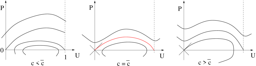
Figure 2: A traveling profile for (2.1) corresponds to a heteroclinic orbit for the system (2.5), connecting the points $(0,0)$ and $(1,0)$. Under the assumptions (A2), such an orbit exists for one specific value $c=c^{*}$.

3 Optimal control of the wave speed

In the setting of Theorem 2.1, consider a speed $c>c^{*}$, so that the equation (2.1) does not admit any traveling profile with speed $c$. Given the function $g$ at (1.7) or (1.8), we then consider the controlled equation

$$u_{t}~{}=~{}f(u)+u_{xx}-g(u,\alpha).$$ (3.1)

Two questions now arise.

• Does there exists a control $\alpha=\alpha(x-ct)\geq 0$ such that (3.1) admits a traveling wave solution with the prescribed speed $c$ ?

• In the positive case, can this be achieved by an optimal control $\alpha(\cdot)$, minimizing the cost $\|\alpha\|_{{\bf L}^{1}}$ ?

Since the above cost has linear growth, to ensure the existence of an optimal solution we must reformulate the problem in a measure-valued setting. Traveling profiles (2.2) thus correspond to solutions of

$$U^{\prime\prime}+cU^{\prime}+f(U)~{}=~{}\mu,$$ (3.2)

with asymptotic conditions

$$U(-\infty)\,=\,0,\quad U(+\infty)\,=\,1.$$ (3.3)

Definition 3.1

By ${\cal M}_{c}$ we denote the set of all positive, bounded Radon measures on the real line, such that the problem (3.2)-(3.3) has a monotonically increasing solution.

More specifically, two optimization problems will be considered.

• Assuming that $f$ satisfies either (A1) or (A2), given a speed $c>c^{*}$, find a measure $\mu\in{\cal M}_{c}$ which minimizes

  $$J_{0}(\mu)\,\doteq\,\mu({\mathbb{R}}).$$ (3.4)

• In the bi-stable case where $f$ satisfies (A2), given a speed $c>c^{*}$, find a measure $\mu\in{\cal M}_{c}$ which minimizes

  $$J_{1}(\mu)\,\doteq\,\int_{{\mathbb{R}}}{1\over u}\,d\mu.$$ (3.5)

3.1 The optimal solution for problem (P1).

Setting $P=U^{\prime}$, a solution to (3.2)-(3.3) corresponds to a solution of

$$\left\{\begin{array}[]{rl}U^{\prime}&=~{}P,\\[2.84526pt] P^{\prime}&=~{}-cP-f(U)+\mu,\end{array}\right.$$ (3.6)

starting at $(0,0)$ and reaching $(1,0)$. Since $f$ is bounded and the measure $\mu$ has finite total mass, any such solution will have bounded total variation.

We observe that, at a point $\bar{x}$ where $\mu$ concentrates a positive mass, the derivative $P$ has an upward jump:

$$U^{\prime}(\bar{x}+)-U^{\prime}(\bar{x}-)~{}=~{}\mu(\{\bar{x}\})~{}>~{}0.$$

Following [10, 25], to the graph

$$\bigl{\{}(U,P)=(U(x),U^{\prime}(x))\,;~{}~{}x\in{\mathbb{R}}\big{\}}$$

we add a (finite or countable) set of vertical segments, at places where $P=U^{\prime}$ has an upward jump. By a suitable parameterization, this yields a Lipschitz curve

$$s~{}\mapsto~{}\gamma(s)~{}=~{}\bigl{(}U(s),P(s)\bigr{)},\qquad\quad s\in[0,\bar{s}],$$ (3.7)

containing the graph of the solution of (3.6).

The cost $J_{0}$ in (3.4) can now be expressed as

$$J_{0}(\gamma)~{}=~{}\int_{0}^{\bar{s}}\left[\Big{(}{f(U)\over P}+c\Big{)}U^{\prime}(s)+P^{\prime}(s)\right]ds~{}=~{}\int_{\gamma}\left[\Big{(}{f(U)\over P}+c\Big{)}dU+dP\right].$$ (3.8)

This is to be minimized over a family ${\cal A}_{c}$ of admissible curves, defined as follows.

Definition 3.2

Given a wave speed $c$, we call ${\cal A}_{c}$ the set of all 1-Lipschitz curves of the form $s\mapsto\gamma(s)=(U(s),P(s)\in{\mathbb{R}}^{2}$ such that, for some interval $[0,\bar{s}]$, one has

$$\gamma(0)=(0,0),\qquad\gamma(\bar{s})=(1,0),\qquad P(s)\geq 0\qquad\hbox{for all}~{}s\in[0,\bar{s}],$$ (3.9)

$$\bigl{|}\gamma(s_{1})-\gamma(s_{2})\bigr{|}~{}\leq~{}|s_{1}-s_{2}|\qquad\hbox{for all}~{}s_{1},s_{2}\in[0,\bar{s}],$$ (3.10)

$$U^{\prime}(s)\,\geq\,0,\qquad P^{\prime}(s)~{}\geq~{}\bigl{(}-f(U(s))-c\bigr{)}U^{\prime}(s)\qquad\hbox{for a.e.~{}}s\in[0,\bar{s}].$$ (3.11)

Following an idea introduced in [21], we use Stokes’ theorem to compute the difference in cost between any two paths $\gamma_{1},\gamma_{2}\in{\cal A}_{c}$. Defining the vector field

$${\bf v}~{}=~{}\left({f(U)\over P}+c\,,~{}1\right),$$

by (3.8) we obtain

$$J_{0}(\gamma_{1})-J_{0}(\gamma_{2})~{}=~{}\left(\int_{\gamma_{1}}-\int_{\gamma_{2}}\right){\bf v}~{}=~{}\left(\int\!\!\!\int_{\Omega^{+}}-\int\!\!\!\int_{\Omega^{-}}\right)\omega.$$ (3.12)

Here

$$\omega~{}=~{}\hbox{curl }{\bf v}~{}=~{}{f(U)\over P^{2}}\,,$$ (3.13)

while $\Omega=\Omega^{+}\cup\Omega^{-}$ is the region enclosed between the two curves. As shown in Fig. 3, we call $\Omega^{+}$ the portion of this region whose boundary is traversed counterclockwise, and $\Omega^{-}$ the portion whose boundary is traversed clockwise, when traveling first along $\gamma_{1}$, then along $\gamma_{2}$.

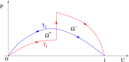
Figure 3: Estimating the difference in cost (3.12) between two paths $\gamma_{1}$ and $\gamma_{2}$.

The formula (3.12) allows to immediately determine the optimal traveling wave profile, for the cost functional $J_{0}$.

• In the monostable case, where $f$ satisfies (1.4), we have $\omega\geq 0$ throughout the domain. As shown in Fig. 4, left, consider the solution of (2.5) through the saddle point $(1,0)$. Since we are assuming $c>c^{*}$, this solution will cross the $P$-axis at some point $b>0$. We then take $\gamma_{1}\in{\cal A}_{c}$ to be the path consisting of a vertical segment from $(0,0)$ to $(0,b)$, together with the trajectory of (2.5) from $(0,b)$ to $(1,0)$. We claim that $\gamma_{1}$ is optimal.

  Indeed, let $\gamma_{2}\in{\cal A}_{c}$ be any other admissible path. Our definition of $\gamma_{1}$ implies that, by moving first along $\gamma_{1}$ then along $\gamma_{2}$, the boundary of the region enclosed by the two curves is traversed clockwise. Hence (3.12) implies

  $$J_{0}(\gamma_{1})-J_{0}(\gamma_{2})~{}=~{}-\int\!\!\!\int_{\Omega^{-}}\omega~{}=~{}-\int\!\!\!\int_{\Omega^{-}}{f(U)\over P^{2}}\,dPdU~{}\leq~{}0.$$ (3.14)

  Hence $\gamma_{1}$ is optimal.

• In the bistable case, where $f$ satisfies (1.5), the function $\omega$ is negative for $u<u^{*}$ and positive for $u>u^{*}$. As shown in Fig. 4, right, let $(u^{*},a)$ be the point reached by the trajectory of (2.5) through $(0,0)$, when it crosses the vertical line $\{U=u^{*}\}$. Similarly, let $(u^{*},b)$ be the point reached by the trajectory of (2.5) through $(1,0)$, when it crosses the vertical line $\{U=u^{*}\}$. Since we are assuming $c>c^{*}$, it follows that $a<b$.

  Define $\gamma_{1}\in{\cal A}_{c}$ to be the path obtained by concatenating these two trajectories, together with a vertical segment joining $(u^{*},a)$ with $(u^{*},b)$. We claim that $\gamma_{1}$ is optimal.

  Indeed, let $\gamma_{2}$ be any other admissible path, connecting $(0,0)$ with $(1,0)$. Our definition of $\gamma_{1}$ implies that, by moving first along $\gamma_{1}$ then along $\gamma_{2}$, the boundary of the region enclosed by the two curves is traversed counterclockwise for $u<u^{*}$ and clockwise for $u>u^{*}$. Hence (3.12) implies

  $$J_{0}(\gamma_{1})-J_{0}(\gamma_{2})~{}=~{}\left(\int\!\!\!\int_{\Omega^{+}}-\int\!\!\!\int_{\Omega^{-}}\right)\omega~{}=~{}\left(\int\!\!\!\int_{\Omega^{+}}-\int\!\!\!\int_{\Omega^{-}}\right){f(U)\over P^{2}}\,dPdU~{}\leq~{}0,$$ (3.15)

  because the ratio $f(U)/P$ is negative on $\Omega^{+}$ and positive on $\Omega^{-}$. Hence $\gamma_{1}$ is optimal.

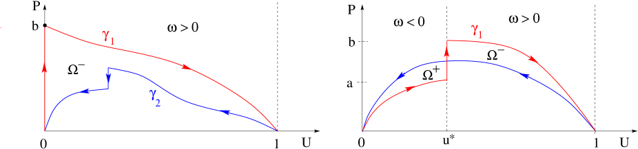
Figure 4: Left: if $f$ is always positive, then the curve $\gamma_{1}$ yields a lower cost, compared with any other admissible curve $\gamma_{2}$. Right: if $f$ is negative for $u<u^{*}$ and positive for $u>u^{*}$, then the curve $\gamma_{1}$ is the optimal one.

We summarize the above analysis, stating the results in the original coordinates $u=u(t,x)$. Consider the problem of minimizing the total mass $\mu({\mathbb{R}})$ among all positive measures for which the equations (3.2)-(3.3) have a solution.

Theorem 3.1

For every $c>c^{*}$, the problem (P1) has a unique solution (up to translations).

• In the monostable case, where $f$ satisfies (1.4), the optimal traveling profile can be uniquely determined by the equations

  $$\left\{\begin{array}[]{rll}U(x)&=~{}0&\hbox{if}~{}~{}x\leq 0,\\[5.69054pt] U^{\prime\prime}+cU^{\prime}+f(U)&=~{}0&\hbox{if}~{}~{}x\leq 0,\\[5.69054pt] \displaystyle\lim_{x\to+\infty}U(x)&=~{}1.\end{array}\right.$$ (3.16)

• In the bistable case, where $f$ satisfies (1.5), the optimal traveling profile can be uniquely determined by the equations

  $$\left\{\begin{array}[]{rl}U^{\prime\prime}+cU^{\prime}+f(U)&=~{}0\qquad\hbox{separately for $x<0$ and for $x>0$},\\[5.69054pt] U(0)&=~{}u^{*},\\[5.69054pt] \lim_{x\to-\infty}U(x)&=~{}0,\qquad\lim_{x\to+\infty}U(x)~{}=~{}1\,.\end{array}\right.$$ (3.17)

In both cases one has $f(u(0))=0$, and the optimal measure $\mu$ is a point mass located at the origin. The minimum cost is

$$C_{min}~{}=~{}\mu\bigl{(}\{0\}\bigr{)}~{}=~{}U^{\prime}(0+)-U^{\prime}(0-).$$ (3.18)

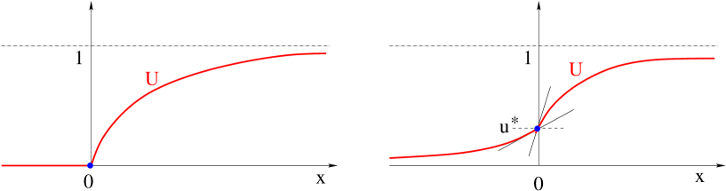
Figure 5: The optimal traveling profiles described in Theorem 3.1. Left: the profile (3.16). Right: the profile (3.17).

3.2 The optimal solution for problem (P2).

Next, consider the bistable case, but with cost functional (3.5). Integrating along paths in the $U$-$P$ plane, instead of (3.8) we now find

$$J_{1}(\gamma)~{}=~{}\int_{0}^{\bar{s}}{1\over U}\left[\Big{(}{f(U)\over P}+c\Big{)}U^{\prime}(s)+P^{\prime}(s)\right]ds~{}=~{}\int_{\gamma}\left[\Big{(}{f(U)\over UP}+{c\over U}\Big{)}dU+{1\over U}dP\right].$$ (3.19)

Again, this is to be minimized among all admissible curves $\gamma\in{\cal A}_{c}$. Defining the vector field

$${\bf v}~{}=~{}\left({f(U)\over UP}+c\,,~{}{1\over U}\right),$$

and recalling (3.19) we now obtain

$$J_{1}(\gamma_{1})-J_{1}(\gamma_{2})~{}=~{}\left(\int_{\gamma_{1}}-\int_{\gamma_{2}}\right){\bf v}~{}=~{}\left(\int\!\!\!\int_{\Omega^{+}}-\int\!\!\!\int_{\Omega^{-}}\right)\omega,$$ (3.20)

where now

$$\omega~{}=~{}\hbox{curl }{\bf v}~{}=~{}{f(U)\over UP^{2}}-{1\over U^{2}}\,.$$ (3.21)

The region where $\omega>0$ is found to be

$${\cal D}^{+}~{}\doteq~{}\Big{\{}(U,P)\,;~{}\omega(U,P)>0\Big{\}}~{}=~{}\Big{\{}(U,P)\,;~{}0<P<P^{*}(U)\Big{\}}.$$ (3.22)

where

$$P^{*}(U)~{}\doteq~{}\sqrt{U\,f(U)}.$$ (3.23)

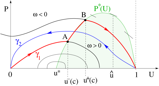
Figure 6: By Stokes’ theorem, the path $\gamma_{1}$ going from $(0,0)$ to $A$, then from $A$ to $B$, then from $B$ to $(1,0)$ has a lower cost than any other admissible path $\gamma_{2}\in{\cal A}_{c}$.

Consider the situation shown in Fig. 6. Let $\gamma_{1}$ be the path obtained by concatenating:

• The trajectory of (2.5) exiting from $(0,0)$, until it reaches a point $A$ on the curve where $P=P^{*}(U)$.

• The trajectory of (2.5) starting from $(1,0)$, and moving backwards until it reaches a point $B$ on the curve where $P=P^{*}(U)$.

• The arc of the curve where $P=P^{*}(U)$, between $A$ and $B$.

Assume that the abode two trajectories of (2.5), passing through the points $A$ and $B$ respectively, do not have further intersections with the curve $P=P^{*}(U)$, for $u^{*}<U<1$. Then $\gamma_{1}$ is optimal.

We give here a sufficient condition that guarantees that every trajectory of (2.5) can cross the curve $P=P^{*}(U)$ only twice, thus ruling out the configuration in Fig. 7.

Along this curve we have

$${d\over dU}{P^{*}(U)}~{}=~{}{f(U)+Uf^{\prime}(U)\over 2\sqrt{Uf(U)}}\,.$$ (3.24)

Writing the equation (3.6) in the form

$$P^{\prime}~{}=~{}-c-{f(U)\over P}+z^{*}(U),$$ (3.25)

a direct computation shows that, in the region where $P=P^{*}$ we must have

$$z^{*}(U)~{}=~{}{3f(U)+Uf^{\prime}(U)\over 2\sqrt{Uf(U)}}+c\,.$$ (3.26)

This leads us to consider the function

$$2g(u)~{}\doteq~{}\bigl{[}3f(u)+uf^{\prime}(u)\bigr{]}\cdot\bigl{[}uf(u)\bigr{]}^{-1/2},$$ (3.27)

and seek a condition that will ensure that this function is monotonically decreasing. A straightforward differentiation yields

$$\begin{array}[]{l}2g^{\prime}(u)~{}=~{}\bigl{[}3f^{\prime}(u)+f^{\prime}(u)+uf^{\prime\prime}(u)\bigr{]}\cdot\bigl{[}uf(u)\bigr{]}^{-1/2}\\[8.53581pt] \qquad\qquad\qquad\displaystyle-{1\over 2}\bigl{(}3f(u)+uf^{\prime}(u)\bigr{)}\bigl{(}f(u)+uf^{\prime}(u)\bigr{)}\cdot\bigl{[}uf(u)\bigr{]}^{-3/2}\\[8.53581pt] \displaystyle~{}=~{}\bigg{[}\Big{(}4uf(u)f^{\prime}(u)+u^{2}f(u)f^{\prime\prime}(u)\Big{)}-{1\over 2}\Big{(}3f^{2}(u)+4uf(u)f^{\prime}(u)+u^{2}(f^{\prime}(u))^{2}\Big{)}\bigg{]}\cdot\bigl{[}uf(u)\bigr{]}^{-3/2}\\[11.38109pt] \displaystyle~{}=~{}\bigg{[}2uf(u)f^{\prime}(u)+u^{2}f(u)f^{\prime\prime}(u)-{3\over 2}f^{2}(u)-{1\over 2}u^{2}(f^{\prime}(u))^{2}\bigg{]}\cdot\bigl{[}uf(u)\bigr{]}^{-3/2}.\end{array}$$

Hence the inequality we need is

$$-3f^{2}(u)-u^{2}(f^{\prime}(u))^{2}+4uf(u)f^{\prime}(u)+2u^{2}f(u)f^{\prime\prime}(u)~{}\leq~{}0.$$ (3.28)

By the inequality $2\sqrt{3}uf(u)f^{\prime}(u)\leq 3f^{2}(u)+u^{2}(f^{\prime}(u))^{2}$, it follows that (3.28) holds if, in addition to (A2), the function $f$ satisfies:

• For all $u\in[u^{*},1]$, one has $(4-2\sqrt{3})f^{\prime}(u)+2uf^{\prime\prime}(u)\leq 0$.

Theorem 3.2

Let $f$ be a function satisfying the assumptions (A2) and (A4) Then the inequality (3.28) holds for every $u\in[0,1]$.

Moreover, for every wave speed $c>c^{*}$, the optimization problem (P2) admits a unique solution. The optimal measure is absolutely continuous w.r.t. Lebesgue measure. There exists two points $u^{*}<u^{-}(c)<u^{+}(c)<1$ such that the optimal solution in (3.25) has the form

$$z^{*}(u)~{}=~{}\left\{\begin{array}[]{cl}\displaystyle{3f(U)+Uf^{\prime}(U)\over 2\sqrt{Uf(U)}}+c&\hbox{if}\quad u\in[u^{-}(c),u^{+}(c)],\\[8.53581pt] 0&\hbox{otherwise.}\end{array}\right.$$ (3.29)

Proof. As shown in Fig. 6, in the region

$$J^{+}~{}\doteq~{}\bigl{\{}u\in[u^{*},1]\,;~{}z^{*}(u)>0\bigr{\}}$$

where the control is strictly positive, the graph of the function $P^{*}$ intersects transversally all trajectories of the system (2.5). Therefore, if we can prove that the set $J^{+}$ is an interval, say $J^{+}=\,]u^{*},\widehat{u}[\,$ as shown in Fig. 6, we are done. We start observing that, under the assumptions (A2) on $f$, the function $z^{*}$ defined at (3.26) satisfies

$$z^{\ast}(u^{\ast})>0\quad\hbox{ and }\quad z^{\ast}(1)<0,$$

hence by continuity of $z^{\ast}$ there exists at least one point $\bar{u}\in[u^{\ast},1]$ such that $z^{\ast}(\bar{u})=0$. We claim that for any $c>c^{*}$ this point is unique. Indeed, consider the function

$$h(u)~{}\doteq~{}-{3\,f(u)+u\,f^{\prime}(u)\over 2\,\sqrt{u\,f(u)}}\,,\qquad\quad u\in[u^{\ast},1].$$ (3.30)

Since

$$\lim_{u\rightarrow u^{*}+}h(u)~{}=\,-\infty,\qquad\qquad\lim_{u\rightarrow 1-}h(u)~{}=\,+\infty\,,$$ (3.31)

our claim will be proved by showing that $h$ is strictly increasing. Indeed, this is true because $h=-g$, with $g$ defined in (3.27).

Remark 3.1

There is a large set of functions satisfying (A2) and (A4). For example, the cubic $f(u)=-x(x-1)(x-2/3)$ satisfies (A4) with a strict inequality. Therefore the same is true for any small perturbation in ${\cal C}^{2}_{0}\bigl{(}[0,1]\bigr{)}$.

4 Existence of optimal traveling profiles

For more general source functions $f$, satisfying (A2) but not (A4) we still prove existence of an optimal measure $\mu$ yielding the traveling profile. However, in the situation shown in Fig. 7 the structure of this measure can be more complicated than in the case covered by Theorem 3.1.

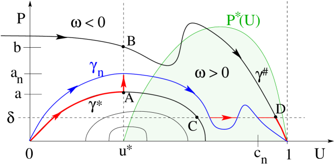
Figure 7: The construction in step 2 of the proof of Theorem 3.2. An admissible path $\gamma_{n}$ is replaced by a path having smaller cost, and having the additional properties (i)–(iii). Notice that this is a case where the trajectory $\gamma^{\sharp}$ of (2.5) through the point $(1,0)$ has multiple intersections with the curve $P=P^{*}(U)$. When this happens, Theorem 3.2 cannot be applied.

Theorem 4.1

Let $f$ satisfy the assumptions (A2), and let $c^{*}$ be the speed of a traveling wave for (2.1). Then, for every $c\geq c^{*}$ the minimization problem (P2) has a measure valued solution.

Proof. 1. As shown in Fig. 7, let $\gamma^{*}$ be the trajectory of (2.5) originating from $(0,0)$, and let $\gamma^{\sharp}$ the trajectory of (2.5) reaching $(1,0)$. Notice that every admissible path $\gamma\in{\cal A}_{c}$ is contained in the region bounded by $\gamma^{*}$, $\gamma^{\sharp}$, and the $U$-axis.

Under the assumption $c\geq c^{*}$, a path with finite cost does exist. Indeed, let $A=(u^{*},a)$ and $B=(u^{*},b)$ be the points where the trajectories $\gamma^{*},\gamma^{\sharp}$ cross the vertical line $\{U=u^{*}\}$, respectively. Then the path $\gamma$ obtained by concatenating

• the portion of $\gamma^{*}$ from $(0,0)$ to $A$,

• the vertical segment from $A$ to $B$, and

• the portion of $\gamma^{\sharp}$ from $B$ to $(1,0)$

is an admissible path with cost $J_{1}(\gamma)={b-a\over u^{*}}<+\infty$. Notice that this is the path that minimizes the cost functional $J_{0}$, but of course it may not be optimal for $J_{1}$. 2. We can now consider a minimizing sequence of paths $\gamma_{n}\in{\cal A}_{c}$, say

$$s~{}\mapsto~{}\gamma_{n}(s)~{}=~{}\bigl{(}U_{n}(s),P_{n}(s)\bigr{)},\qquad s\in[0,s_{n}],\quad n\geq 1,$$

such that

$$\lim_{n\to\infty}~{}J_{1}(\gamma_{n})~{}=~{}\inf_{\gamma\in{\cal A}_{c}}J_{1}(\gamma).$$

Adapting the arguments used in the previous section, based on Stokes’ theorem, we now replace each path $\gamma_{n}$ with a modified path $\widetilde{\gamma}_{n}$ having some additional properties. As shown in Fig. 7, let $(u^{*},a_{n})$ be the first point where the path $\gamma_{n}$ intersects the vertical line $U=u^{*}$. We can then replace the portion of $\gamma_{n}$ between $(0,0)$ and $(u^{*},a)$ with the portion of $\gamma^{*}$ from $(0,0)$ to the point $A=(u^{*},a)$, together with a vertical segment joining $(u^{*},a)$ with $(u^{*},a_{n})$.

Next, consider the portion of $\gamma_{n}$ in a neighborhood of the terminal point $(1,0)$. Since the measure $\mu$ is positive, that this portion must lie below the trajectory $\gamma^{\sharp}$ of (2.5) through $(1,0)$. Moreover, in a neighborhood of $(1,0)$ the path $\gamma^{\sharp}$ lies below the curve $P=P^{*}(U)$. Indeed, in view of (3.24),

$$\lim_{U\to 1-}{d\over dU}P^{*}(U)~{}=~{}\lim_{U\to 1-}\left({\sqrt{f(U)}\over 2U}+{\sqrt{U}\,f^{\prime}(U)\over 2f(U)}\right)~{}=~{}-\infty,$$

while, along $\gamma^{\sharp}$, by (2.6)-(2.7) we have

$$\lim_{U\to 1-}{dP\over dU}~{}=~{}{-c-\sqrt{c^{2}-4f^{\prime}(1)}\over 2}\,.$$

We now choose $\delta>0$ small enough so that, calling $C,D$ the points where the horizontal line $\{P=\delta\}$ intersects the trajectories $\gamma^{*}$ and $\gamma^{\sharp}$ respectively, one has

$$-f(U)-cP~{}\leq~{}0$$

along the horizontal segment with endpoints $C,D$. In other words, all trajectories of (2.5) cross this segment downward.

Call $(c_{n},\delta)$ the last point where the path $\gamma_{n}$ crosses the horizontal line $\{P=\delta\}$. We then replace the last portion of $\gamma_{n}$ with a horizontal segment joining $(c_{n},\delta)$ with $D$, together with the portion of trajectory $\gamma^{\sharp}$ joining $D$ with $(1,0)$. Furthermore, we replace any additional portions of the path $\gamma_{n}$ lying below the line $\{P=\delta\}$ with horizontal segments.

After these modifications, we obtain a new path $\widetilde{\gamma}_{n}$. Since the function $\omega$ at (3.21) is negative on the strip where $U<u^{*}$, by (3.15) we have

$$J_{1}(\widetilde{\gamma}_{n})\,\leq\,J_{1}(\gamma_{n}).$$

In view of the above construction we can now assume that every path $\gamma_{n}$ in our minimizing sequence has the following properties:

• The initial portion of $\gamma_{n}$ coincides with the path $\gamma^{*}$, from $(0,0)$ to the point $A=(u^{*},a)$.

• The final portion of $\gamma_{n}$ coincides with the path $\gamma^{\sharp}$, from the point $D$ to $(1,0)$.

• The intermediate portion of $\gamma_{n}$, between $A$ and $D$, remains inside the domain where $U\in[u^{*},1]$ and $P\geq\delta$.

3. By parameterizing each path $\gamma_{n}$ by arc-length, we can assume that all maps $\gamma_{n}$ are 1-Lipschitz and that the intervals $[0,s_{n}]$ are uniformly bounded. By possibly taking a subsequence, and using Ascoli’s theorem, we achieve the convergence

$$s_{n}\to\bar{s},\qquad\gamma_{n}(s)\to\gamma(s)\qquad\hbox{for all}~{}s\in[0,\bar{s}[\,.$$

Moreover, for any fixed $\varepsilon>0$ the convergence is uniform on the subinterval where $s\in[0,\bar{s}-\varepsilon]$. 4. We claim that the limit path is admissible, namely $\gamma\in{\cal A}_{c}$. Indeed, the identities (3.9) are clear. Moreover, the limit of 1-Lipschitz curves is still 1-Lipschitz, hence (3.10) holds as well. Finally, we observe that the differential constraint (3.11) can be formulated in terms of the differential inclusion

$$\gamma^{\prime}(s)~{}\in~{}F(\gamma(s)),$$ (4.1)

where

$$F(U,P)~{}=~{}\Big{\{}(\dot{u},\dot{p})\in{\mathbb{R}}^{2}\,;~{}\dot{u}^{2}+\dot{p}^{2}\leq 1\,,\quad\dot{u}\geq 0,~{}~{}\dot{p}~{}\geq~{}(-f(U)-c)\dot{u}\Big{\}}.$$

Since the multifunction $F$ is continuous, with compact, convex values, the set of solutions to the differential inclusion (4.1) is closed under uniform convergence [1]. This shows that $\gamma\in{\cal A}_{c}$. 4. It now remains to show that the limit path $\gamma$ is optimal. Namely

$$J_{1}(\gamma)~{}=~{}\int_{\gamma}\left[\Big{(}{f(U)\over UP}+{c\over U}\Big{)}dU+{1\over U}dP\right]~{}=~{}\lim_{n\to\infty}J_{1}(\gamma_{n}).$$ (4.2)

Using (3.15)-(3.21) we obtain

$$\lim_{n\to\infty}\Big{(}J_{1}(\gamma)-J_{1}(\gamma_{n})\Big{)}~{}=~{}\lim_{n\to\infty}\left(\int\!\!\!\int_{\Omega^{+}_{n}}-\int\!\!\!\int_{\Omega^{-}_{n}}\right)\left({f(U)\over UP^{2}}-{1\over U^{2}}\right)~{}=~{}0.$$ (4.3)

Indeed, by construction, for every $n\geq 1$ the region $\Omega_{n}=\Omega_{n}^{+}\cup\Omega_{n}^{-}$ enclosed between the two curves is contained within the region where $U\geq u^{*}$ and $P\geq\delta$. On this region, the integrand in (4.3) is continuous and uniformly bounded. Since the area of $\Omega_{n}$ shrinks to zero, we conclude that the above limit vanishes, proving the optimality of $\gamma$.MM     

The above theorem provides the existence of an optimal profile, but it does not guarantee its uniqueness (up to translation). From step 2 of the proof, we can obtain some information about the optimal measure $\mu$. Namely $\mu$ is supported on a region where $U\in[u^{*},1-\varepsilon]$, for some $\varepsilon>0$. In particular, the optimal profile coincides with a solution of (2.3) for $U\in\,]0,u^{*}]$ and for $U\in[1-\varepsilon,1[\,$.

5 The minimum cost, depending on the wave speed

In setting considered in Theorem 3.2, the optimal control has the form (3.29). Calling $[u^{-}(c),u^{+}(c)]$ the interval where the control is nonzero (see Fig. 6), the minimum cost is thus

$$\begin{array}[]{rl}E(c)&\displaystyle=~{}\int_{u^{-}(c)}^{u^{+}(c)}{z^{*}(u)\over u}\,du~{}=~{}\int_{u^{-}(c)}^{u^{+}(c)}{3f(u)+uf^{\prime}(u)+2c\sqrt{uf(u)}\over 2u\sqrt{uf(u)}}\,du\\[11.38109pt] &\displaystyle=~{}{3\over 2}\int_{u^{-}(c)}^{u^{+}(c)}{\sqrt{f(u)}\over u\sqrt{u}}\,du+{1\over 2}\int_{u^{-}(c)}^{u^{+}(c)}{f^{\prime}(u)\over\sqrt{uf(u)}}\,\,du+c\ln\left({u^{+}(c)\over u^{-}(c)}\right).\end{array}$$ (5.1)

The first two terms on the right hand side of (5.1) are uniformly bounded. The last term is the only one that grows without bound, as $c\to+\infty$. The next proposition yields more precise information on the asymptotic behavior of $E(c)$.

Proposition 5.1

Let $f$ be a function satisfying the assumptions (A2) and (A4). As in Theorem 3.2, let $z^{*}$ in (3.29) be the optimal control for the problem (P2). Then, as $c\to+\infty$, one has $u^{-}(c)\to u^{*}$, $u^{+}(c)\to 1$. Moreover, the function $E(c)$ in (5.1) has the asymptotic behavior

$$E(c)~{}=~{}c\,|\ln u^{*}|+\int_{u^{*}}^{1}\left({3\sqrt{f(u)}\over 2u\sqrt{u}}+{f^{\prime}(u)\over 2\sqrt{uf(u)}}\right)du+e(c),$$ (5.2)

where the additional term has size $e(c)={\cal O}(1)\cdot{1\over c}$.

Proof. All of the above conclusions will be proved by showing that there exists a constant $\alpha>0$ such that

$$u^{-}(c)-u^{*}~{}\leq~{}{\alpha\over c^{2}}\,,\qquad\qquad 1-u^{-}(c)~{}\leq~{}{\alpha\over c^{2}}\,.$$ (5.3)

1. Consider the equation

$${dP\over dU}~{}=~{}-c-{f(U)\over P},\,$$ (5.4)

associated with the system (2.5). One can observe that for $c>0$,

$${dP\over dU}~{}\leq~{}-c\qquad\hbox{ on }\text{ }[u^{\ast},1].$$ (5.5)

Therefore $P$ attains its maximum at some point in the interval $[0,u^{\ast}]$, where the right hand side of (5.4) vanishes. For $u\in[0,u^{*}]$ one has $f_{\text{min}}\leq f(u)\leq 0$. Therefore

$$0~{}\leq~{}P(U)~{}\leq~{}-{f_{\text{min}}\over c}\qquad\qquad\hbox{for all}~{}U\in[0,1].$$ (5.6)

In turn, (5.6) implies

$$-{f_{min}\over c}~{}\geq~{}\sqrt{{u^{-}(c)f(u^{-}(c))}}.$$ (5.7)

As $c\to+\infty$, both sides of (5.7) approach zero, hence $f(u^{-}(c))\to 0$ and $u^{-}(c)\to u^{*}$. Moreover, performing a Taylor approximation at $u=u^{*}$, for a suitable constant $\alpha>0$ we find

$$\sqrt{u^{-}(c)-u^{*}}~{}\leq~{}{\sqrt{\alpha}\over c}\,.$$ (5.8)

proving the first inequality in (5.3).

2. To achieve an estimate on $u^{+}(c)$ we observe that, for every $c>0$, the function

$$Z(U)~{}=~{}c(1-U)\qquad\qquad U\in[u^{*},1]\,,$$

is a subsolution of

$${d\over dU}P(U)~{}=~{}-c-{f(U)\over P}\,,\qquad\qquad P(1)=0.$$

Indeed,

$$Z^{\prime}~{}=~{}-c~{}\geq~{}-c-{f(U)\over Z}\qquad\qquad U\in[u^{*},1]\,.$$

In turn, this implies

$$P^{*}(u^{+}(c))~{}=~{}\sqrt{u^{+}(c))f(u^{+}(c))}~{}\geq~{}Z(u^{+}(c))~{}=~{}c\bigl{(}1-u^{+}(c)\bigr{)}.$$

Once again, for a suitable constant $\alpha>0$ this implies

$$\sqrt{\alpha(1-u^{+}(c))}~{}\geq~{}c\bigl{(}1-u^{+}(c)\bigr{)},$$

proving the second inequality in (5.3). 3. The asymptotic expansion (5.2) is now a consequence of (5.1), together with the inequalities in (5.3). MM     

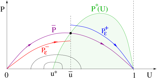
Figure 8: When $c=c^{*}$ there exists a heteroclinic orbit $P=\overline{P}(U)$ of (2.5) through $(0,0)$ and $(1,0)$. When $c=c^{*}+\varepsilon$ with $\varepsilon>0$, one obtains an unstable manifold $P=P^{-}_{\varepsilon}(U)$ through $(0,0)$, and a stable manifold $P=P^{+}_{\varepsilon}(U)$ through $(1,0)$.

Next, we analyze the behavior of $E(c)$ as $c\downarrow c^{*}$. Going back to the system (2.5), we observe that the unstable manifold through $(0,0)$ and the stable manifold through $(1,0)$ depend continuously on the parameter $c$. This impliies

$$\lim_{c\to c^{*}}u^{-}(c)~{}=~{}\lim_{c\to c^{*}}u^{+}(c)~{}=~{}\bar{u}.$$ (5.9)

As shown in Fig. 8, here $\bar{u}$ is the point where the heteroclicic orbit $P=\overline{P}(U)$ connecting $(0,0)$ with $(1,0)$ intersects the graph of the function $P=P^{*}(U)\doteq\sqrt{Uf(U)}$, in the case $c=c^{*}$.

Setting $c=c^{*}+\varepsilon$, we now denote by $P=P^{-}_{\varepsilon}(U)$ and $P=P^{+}_{\varepsilon}(U)$ the corresponding unstable and stable manifolds through $(0,0)$ and $(1,0)$, respectively (see Fig. 8). By definition, the functions $P^{-}_{\varepsilon},P^{+}_{\varepsilon}$ thus provide the solutions to

$${dP\over dU}~{}=~{}-{f(U)\over P}-(c^{*}+\varepsilon),$$ (5.10)

respectively with boundary conditions

$$P_{\varepsilon}^{-}(0)~{}=~{}0,\qquad\qquad P_{\varepsilon}^{+}(1)~{}=~{}0.$$

Differentiating (5.10) w.r.t. the parameter $\varepsilon$, we obtain the asymptotic expansions

$$P^{-}_{\varepsilon}(U)~{}=~{}\overline{P}(U)+\varepsilon Y^{-}(U)+o(\varepsilon),\qquad\qquad P^{+}_{\varepsilon}(U)~{}=~{}\overline{P}(U)+\varepsilon Y^{+}(U)+o(\varepsilon),$$ (5.11)

where $o(\varepsilon)$ denotes a higher order term, as $\varepsilon\to 0$. Here the functions $Y^{-},Y^{+}$ are determined by solving the linearized equations

$${dY\over dU}~{}=~{}{f(U)\over[\overline{P}(U)]^{2}}\,Y-1,$$ (5.12)

with boundary conditions

$$\lim_{U\to 0+}Y^{-}(U)~{}=~{}0,\qquad\qquad\lim_{U\to 1-}Y^{+}(U)~{}=~{}0,$$

respectively. In view of the formula (5.1), we now obtain

Proposition 5.2

In the same setting as Proposition 5.1, we have the asymptotic expansion

$$E(c^{*}+\varepsilon)~{}=~{}\varepsilon\cdot{Y^{+}(\bar{u})-Y^{-}(\bar{u})\over\bar{u}}+o(\varepsilon).$$ (5.13)

where $o(e)$ denotes a higher order infinitesimal as $\varepsilon\downarrow 0$.

Proof. For notational convenience, set

$$v^{-}~{}\doteq~{}{d\over d\varepsilon}u^{-}(c^{*}+\varepsilon)\bigg{|}_{\varepsilon=0}\,,\qquad\qquad v^{+}~{}\doteq~{}{d\over d\varepsilon}u^{+}(c^{*}+\varepsilon)\bigg{|}_{\varepsilon=0}\,.$$

Differentiating w.r.t. $\varepsilon$ the identities

$$P_{\varepsilon}^{-}\bigl{(}u^{-}(c^{*}+\varepsilon)\bigr{)}~{}=~{}P^{*}\bigl{(}u^{-}(c^{*}+\varepsilon)\bigr{)},\qquad\qquad P_{\varepsilon}^{+}\bigl{(}u^{-}(c^{*}+\varepsilon)\bigr{)}~{}=~{}P^{*}\bigl{(}u^{+}(c^{*}+\varepsilon)\bigr{)},$$

and using (5.11), we obtain

$$Y^{\pm}(\bar{u})+\left(-c^{*}-{f(\bar{u})\over\bar{u}}\right)v^{\pm}~{}=~{}(P^{*})^{\prime}(\bar{u})\cdot v^{\pm}.$$ (5.14)

It is now convenient to write the minimum cost (5.1) in the form

$$E(c)~{}=~{}\int_{u^{-}(c)}^{u^{+}(c)}{z^{*}(u)\over u}\,du~{}=~{}\int_{u^{-}(c)}^{u^{+}(c)}{1\over u}\left(c+{f(u)\over P^{*}(u)}+(P^{*})^{\prime}(u)\right)\,du\,.$$ (5.15)

Differentiating (5.15) w.r.t. $c$, when $c=c^{*}$ and $u^{-}(c^{*})=u^{+}(c^{*})=\bar{u}$ we obtain

$$E^{\prime}(c^{*})~{}=~{}{1\over\bar{u}}\left(c^{*}+{f(\bar{u})\over P^{*}(\bar{u})}+(P^{*})^{\prime}(\bar{u})\right)\cdot(v^{+}-v^{-})~{}=~{}{Y^{+}(\bar{u})-Y^{-}(\bar{u})\over\bar{u}}\,,$$

where the second identity follows from (5.14). This yields (5.13). MM     

The last result in this section is concerned with minimum cost $J_{0}$ in (3.4), as a function of the wave speed $c$, but now in the mono-stable case (1.4). In this case, we can prove that the function $E(c)$ is convex.

Proposition 5.3

Consider the minimization problem (P1), assuming that $f$ satisfies (A1). Then the minimum cost $E(c)$ is an increasing, convex function of the speed $c\in[c^{*},+\infty[\,$.

Proof. As shown by Theorem 3.1, in this case the optimal control consists of a point mass at the origin. The minimum cost is thus simply $P(0)$, where $P=P(U)$ is the solution to

$${dP\over dU}~{}=~{}-cP-{f(U)\over P},\qquad\qquad P(1)=0.$$ (5.16)

We shall write $P=P(U,c)$ to emphasize the dependence of the solution on the additional parameter $c$. Our main concern is the convexity of the map $c\mapsto P(0,c)$. To understand this issue, we set  $w={\partial P\over\partial c}$. This function satisfies the linear ODE

$${dw\over dU}~{}=~{}-1+{f(U)\over P^{2}(U)}\,w,\qquad\qquad w(1)=0.$$ (5.17)

If now $c_{1}<c_{2}$, then $P(U,c_{1})<P(U,c_{2})$. Therefore

$$-1+{f(U)\over P^{2}(U,c_{1})}~{}>~{}-1+{f(U)\over P^{2}(U,c_{2})}\,.$$

In view of (5.17), this yields

$$w(U,c_{1})~{}<~{}w(U,c_{2})\qquad\qquad\hbox{for all}~{}U\in[0,1[\,.$$ (5.18)

showing that the map $c\mapsto P(U,c)$ is convex, for every $U\in[0,1]$. MM     

6 Traveling profiles in two space dimensions

In Theorem 3.1 we proved that, for any speed $c>c^{*}$, the optimization problem (P1) admits a unique optimal solution. The optimal measure is a point mass located at a point where $f(u)=0$.

Aim of this section is to prove a similar result for traveling waves in two space dimensions. We thus consider the corresponding parabolic equation on the 2-dimensional strip $\bigl{\{}(x_{1},x_{2})\in{\mathbb{R}}\times\,]0,1[\,\bigr{\}}$, namely

$$u_{t}~{}=~{}f(u)+\Delta u-z(x),$$ (6.1)

with Neumann boundary conditions:

$$u_{x_{2}}(x_{1},0)~{}=~{}u_{x_{2}}(x_{1},1)~{}=~{}0\qquad\hbox{for all}~{}x_{1}\in{\mathbb{R}}.$$ (6.2)

Given a speed $c>c^{*}$, we consider a traveling wave profile $u=u(x_{1},x_{2})$ which satisfies

$$f(u)+cu_{x_{1}}+\Delta u-z~{}=~{}0,$$ (6.3)

together with (6.2) and with limits

$$\lim_{x_{1}\to-\infty}u(x_{1},x_{2})~{}=~{}0,\qquad\lim_{x_{1}\to+\infty}u(x_{1},x_{2})~{}=~{}1.$$ (6.4)

Among all such profiles, obtained by different choices of the function $z=z(x_{1},x_{2})\geq 0$, we seek to minimize the total effort

$$\|z\|_{{\bf L}^{1}}~{}\doteq~{}\int_{{\mathbb{R}}\times[0,1]}\bigl{|}z(x)\bigr{|}\,dx.$$ (6.5)

We claim that, even by choosing control functions $z$ which depend on both variables $x_{1},x_{2}$, one cannot achieve a smaller cost compared with the 1-dimensional case, where $z$ is a function of the variable $x_{1}$ alone.

Proposition 6.1

Let $f$ satisfy the assumptions (A1). Given $c>c^{*}$, let $u=u(x_{1},x_{2})$ be a solution to (6.2)–(6.4), for some nonnegative smooth function $z=z(x_{1},x_{2})$. Calling $C_{min}$ the minimum cost for the 1-dimensional problem at (3.18), one has

$$\|z\|_{{\bf L}^{1}}~{}\geq~{}C_{min}\,.$$ (6.6)

Proof. 1. By (6.3) and the boundary conditions (6.2), (6.4), one has

$$\|z\|_{{\bf L}^{1}}~{}=~{}\int_{{\mathbb{R}}\times[0,1]}f(u)\,dx+c.$$ (6.7)

Introducing the level sets

$$\Sigma(s)~{}\doteq~{}\Big{\{}x\in{\mathbb{R}}\times[0,1]\,;~{}u(x)=s\Big{\}},$$

the integral on the right hand side of (6.7) can be written as

$$\int_{0}^{1}\left(\int_{\Sigma(s)}{1\over|\nabla u(x)|}\,d\ell\right)f(s)\,ds.$$ (6.8)

Here $d\ell$ denotes the arc-length along the level curve $\Sigma(s)$. 2. Assuming that $f$ satisfies (1.4), let $U:{\mathbb{R}}_{+}\mapsto[0,1]$ be the optimal traveling profile constructed at (3.16). For every $s\in[0,1]$, define

$$\psi(s)~{}\doteq~{}\int_{\{u(x)>s\}}f(u(x))\,dx,\qquad\qquad\Psi(s)~{}\doteq~{}\int_{\{U(x)>s\}}f(U(x))\,dx\,.$$ (6.9)

We claim that, for every $s\in[0,1]$,

$$\psi(s)~{}\geq~{}\Psi(s).$$ (6.10)

Toward a proof of (6.10) we shall use the divergence theorem on the set $\{u(x)>s\}$. Choosing ${\bf n}=\nabla u/|\nabla u|$ as inner unit normal vector, by (6.1) we have

$$\int_{\Sigma(s)}|\nabla u|\,d\ell~{}=~{}\int_{\Sigma(s)}\nabla u\cdot{\bf n}\,d\ell~{}=~{}-\int_{\{u(x)>s\}}\Delta u\,dx~{}=~{}\int_{\{u(x)>s\}}\bigl{(}f(u)+cu_{x_{1}}-z\bigr{)}\,dx$$ (6.11)

The inequality (6.10) trivially holds when $s=1$, because in this case both sides vanish. Let us decrease $s$ and check at what rate the two integrals increase. Taking the average values, and applying Jensen’s inequality for the convex function $y\mapsto 1/y$, for any $c\in{\mathbb{R}}$ we obtain

$$\begin{array}[]{rl}\displaystyle-{d\over ds}\psi(s)&\displaystyle=~{}f(s)\cdot\int_{\Sigma(s)}{1\over|\nabla u(x)|}\,d\ell(s)\\[11.38109pt] &\displaystyle=~{}f(s)\cdot\hbox{meas}\bigl{(}\Sigma(s)\bigr{)}\cdot-\!\!\!\!\!\!\!\int_{\Sigma(s)}{1\over|\nabla u(x)|}\,d\ell(s)\\[11.38109pt] &\displaystyle\geq~{}f(s)\cdot\hbox{meas}\bigl{(}\Sigma(s)\bigr{)}\cdot\left(-\!\!\!\!\!\!\!\int_{\Sigma(s)}|\nabla u(x)|\,d\ell(s)\right)^{-1}\\[11.38109pt] &\displaystyle=~{}f(s)\cdot\Big{[}\hbox{meas}\bigl{(}\Sigma(s)\bigr{)}\Big{]}^{2}\cdot\left(\int_{\{u(x)>s\}}(f(u)+cu_{x_{1}}-z)\,dx\right)^{-1}\\[11.38109pt] &\geq~{}f(s)\cdot\Big{[}\hbox{meas}\bigl{(}\Sigma(s)\bigr{)}\Big{]}^{2}\cdot\bigl{[}\psi(s)+c(1-s)\bigr{]}^{-1},\end{array}$$ (6.12)

$$\begin{array}[]{rl}\displaystyle-{d\over ds}\Psi(s)&\displaystyle=~{}{f(s)\over U^{\prime}(x(s))}~{}=~{}f(s)\cdot\left[\int_{x(s)}^{+\infty}f(U(x))\,dx+c(1-s)\right]^{-1}\\[11.38109pt] &\displaystyle=~{}f(s)\cdot\bigl{[}\Psi(s)+c(1-s)\bigr{]}^{-1}.\end{array}$$ (6.13)

Comparing (6.12) with (6.13), we see that

• either  $\psi(s)\geq\Psi(s)$,

• or else   $\displaystyle-{d\over ds}\psi(s)~{}\geq~{}-{d\over ds}\Psi(s)$.

Since $\psi(1)=\Psi(1)=0$, letting $s$ decrease from 1 to 0 by a comparison argument we conclude that (6.10) holds. MM     

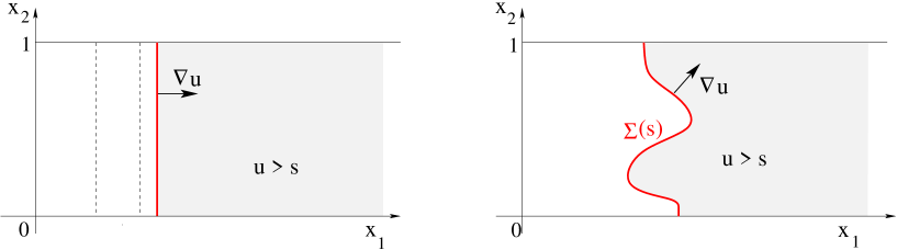
Figure 9: Left: the regions where $u(x_{1},x_{2})=U(x_{1})$ is $>s$. Right: the region where a general solution $u$ of (6.3) is $>s$.

7 The two-dimensional sharp interface limit

We now return to the optimization problem introduced in Section 1, but with a possibly measure-valued dissipative source:

$$u_{t}~{}=~{}f(u)+\Delta u-\mu\,.$$ (7.1)

We are interested in the sharp interface limit, obtained by letting $\varepsilon\to 0$ in the equation

$$u_{t}~{}=~{}{1\over\varepsilon}f(u)+\varepsilon\,\Delta u-\mu\,.$$ (7.2)

Notice that (7.2) can be derived from (7.1) simply by a rescaling of the independent variables $t\mapsto\varepsilon t$, $x\mapsto\varepsilon x$. Here $\mu$ as a (possibly measure-valued) non-negative control. For $\varepsilon\approx 0$ we expect that the solution to (7.2) will be a function taking values close to either 0 or 1 over most of its domain. We thus seek to replace the controlled parabolic equation (7.2) with a control problem for a moving set.

The following notation will be used. On the unit circumference $S=\{\xi\in{\mathbb{R}}^{2}\,;~{}|\xi|=1\}$ we use the arc-length measure, normalized so that $\int_{S}d\xi=1$. For any vector $v=(v_{1},v_{2})\in{\mathbb{R}}^{2}$, the perpendicular vector (rotated by $90^{o}$) is $v^{\perp}=(-v_{2},v_{1})$. By ${\bf 1}_{V}$ we denote the characteristic function of a set $V\subset{\mathbb{R}}^{2}$, while $m_{2}(V)$ denotes its 2-dimensional Lebesgue measure.

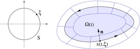
Figure 10: At time $t$, the boundary $\partial\Omega(t)$ of the moving set is parameterized by the variable $\xi\in S^{1}$. An annulus of radius $\varepsilon^{1/2}$ around this boundary is parameterized by $(\xi,s)\mapsto x(t,\xi)+s{\bf n}(t,\xi)$.

Consider a set valued map $t\mapsto\Omega(t)\subset{\mathbb{R}}^{2}$. For $t\in[0,T]$, let

$$\partial\Omega(t)~{}=~{}\{x(t,\xi)\,;~{}\xi\in S\}$$ (7.3)

be a ${\cal C}^{1}$ parameterization of the boundary of $\Omega(t)$, oriented counterclockwise (see Fig. 10). We shall always assume that $x_{\xi}(t,x)\not=0$ for all $t,\xi$, so that the unit inward normal vector to $\Omega(t)$ at $x(t,\xi)$ is well defined by the formula

$${\bf n}(t,\xi)~{}\doteq~{}{x_{\xi}^{\perp}(t,\xi)\over|x_{\xi}(t,\xi)|}\,.$$ (7.4)

The normal velocity of the set boundary is given by the inner product

$$\beta(t,\xi)~{}\doteq~{}\big{\langle}{\bf n}(t,\xi)\,,\,x_{t}(t,\xi)\big{\rangle}.$$ (7.5)

Throughout this section, we assume that the source function $f$ satisfies (A2) and (A4), so that Theorem 3.2 applies. In connection with the optimization problem (P2) for a traveling wave, for every speed $c\geq c^{*}$ let $E(c)$ in (5.1) be the minimum cost (3.5), among all measure-valued controls yielding a traveling profile with speed $c$. One can extend $E$ to all values $c\in{\mathbb{R}}$ by setting

$$E(c)\,=\,0\qquad\hbox{for}\qquad c\leq c^{*}.$$

Integrating this cost along the boundary of a moving set, this leads to

Definition 7.1

Consider a moving set $\Omega(t)$, with boundary parameterized as in (7.3). At each time $t\in[0,T]$, the instantaneous effort to achieve this motion is defined as

$${\cal E}(t)~{}\doteq~{}\int_{S}E(\beta(t,\xi))\,\bigl{|}x_{\xi}(t,\xi)\bigr{|}\,d\xi\,.$$ (7.6)

Given a convex function $\phi:{\mathbb{R}}_{+}\,\mapsto{\mathbb{R}}_{+}$ and two constants $\kappa_{1},\kappa_{2}\geq 0$, together with the optimization problem (OP1) introduced in Section 1, we now consider a problem of optimal control for the moving set $\Omega(t)$, $t\in[0,T]$.

• Given an initial set $\Omega(0)=\Omega_{0}$, determine a controlled evolution $t\mapsto\Omega(t)$ so that the total cost

  $$J~{}\doteq~{}\int_{0}^{T}\phi\bigl{(}{\cal E}(t)\bigr{)}\,dt+\kappa_{1}\int_{0}^{T}m_{2}\bigl{(}\Omega(t)\bigr{)}\,dt+\kappa_{2}\,m_{2}\bigl{(}\Omega(T)\bigr{)}$$ (7.7)

  is minimized.

A rigorous derivation of (OP2) would require a study of the $\Gamma$-limit of the functionals

$${\cal F}_{\varepsilon}(u)~{}\doteq~{}\int_{0}^{T}\int{[\varepsilon\Delta u+\varepsilon^{-1}f(u)-u_{t}]_{+}\over u}\,dx\,dt$$ (7.8)

as $\varepsilon\to 0$. Here $[s]_{+}=\max\{s,0\}$. However, this analysis is outside the scope of the present paper. Here we only take some partial steps in this direction. The main result of this section shows that the cost $J$ at (7.7) can be achieved as the limit of the cost (1.2), for a family of solutions to the rescaled parabolic equations

$$u^{\varepsilon}_{t}~{}=~{}{1\over\varepsilon}f(u^{\varepsilon})+\varepsilon\,\Delta u^{\varepsilon}-u^{\varepsilon}\alpha^{\varepsilon}\,,\qquad\qquad t\in[0,T],~{}x\in{\mathbb{R}}^{2}.$$ (7.9)

Theorem 7.1

Let $f$ satisfy the assumptions (A2)-(A3). For $t\in[0,T]$, let $t\mapsto\Omega(t)\subset{\mathbb{R}}^{2}$ denote a moving set, whose boundary admits a ${\cal C}^{1}$ parameterization as in (7.3). Moreover, assume that the normal velocity in (7.5) satisfies $\beta(t,\xi)\geq c^{*}$ for all $t,\xi$. Then there exists a family of control functions $\alpha^{\varepsilon}$ and solutions $u^{\varepsilon}$ to (7.9) such that the following two limits hold, uniformly for $t\in[0,T]$.

$$\lim_{\varepsilon\to 0}\Big{\|}u^{\varepsilon}(t,\cdot)-{\bf 1}_{\Omega(t)}\Big{\|}_{{\bf L}^{1}}~{}=~{}0,$$ (7.10)

$$\lim_{\varepsilon\to 0}\int_{{\mathbb{R}}^{2}}\alpha^{\varepsilon}(t,x)\,dx~{}=~{}\int_{S^{1}}E\bigl{(}\beta(t,\xi)\bigr{)}\,\bigl{|}x_{\xi}(t,\xi)\bigr{|}\,d\xi.$$ (7.11)

Proof. 1. By an approximation argument, we can assume that the function $x=x(t,\xi)$ is smooth, and that the normal speeds satisfy the strict inequality $\beta(t,\xi)>c^{*}$. More precisely, we can choose constants $c_{1},c_{2},c_{3}$ such that

$$c^{*}\,<c_{1}\,<c_{2}\,<\,c_{3},\qquad\qquad\beta(t,\xi)\,\in\,[c_{2},c_{3}]\quad\hbox{for all}~{}t\in[0,T],~{}\xi\in S.$$ (7.12)

The solutions $u^{\varepsilon}$ will be obtained by constructing suitable lower and upper solutions $u^{\varepsilon}_{-}\leq u^{\varepsilon}_{+}$.

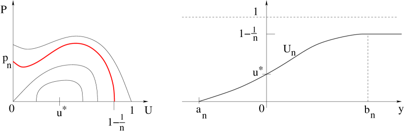
Figure 11: The construction of lower solutions. Left: the trajectory of (7.13) through the point $(1-n^{-1},0)$ crosses the $P$-axis at some point $(0,p_{n})$. Right: the corresponding traveling profile at (7.15)-(7.16) is uniquely determined by requiring that $U_{n}(0)=u^{*}$. By construction we have $U_{n}^{\prime}(a_{n})=p_{n}>0$, while $U_{n}^{\prime}(b_{n})=0$.

2. Toward the construction of lower solutions (see Fig. 11), let $c_{1}>c^{*}$ be given. For every $n\geq 1$ large enough, the trajectory of the system

$$\left\{\begin{array}[]{rl}U^{\prime}&=~{}P,\\[2.84526pt] P^{\prime}&=~{}-f(U)-c_{1}P,\end{array}\right.$$ (7.13)

that goes through the point $(1-n^{-1},\,0)$ will cross the $P$-axis at a point $(0,p_{n})$, with

$$p_{n}\,>\,0,\qquad\lim_{n\to\infty}p_{n}~{}=~{}\bar{p}~{}>~{}0.$$ (7.14)

This yields a traveling profile $U_{n}=U_{n}(y)$ which satisfies

$$U_{n}(0)=u^{*},\qquad\qquad U_{n}^{\prime\prime}+c_{3}U_{n}^{\prime}+f(U_{n})~{}=~{}0\quad\hbox{for}~{}~{}y\in[a_{n},b_{n}],$$ (7.15)

$$\left\{\begin{array}[]{rl}U_{n}(a_{n})&=~{}0,\\[5.69054pt] U^{\prime}_{n}(a_{n})&=~{}p_{n}~{}>~{}0,\end{array}\right.\qquad\left\{\begin{array}[]{rl}U_{n}(b_{n})&=~{}1-{1\over n},\\[5.69054pt] U^{\prime}_{n}(b_{n})&=~{}0,\end{array}\right.$$ (7.16)

for some values $a_{n}<0<b_{n}$. We can extend it outside the interval $[a_{n},b_{n}]$ by setting

$$U_{n}(y)~{}=~{}\left\{\begin{array}[]{cl}0&\hbox{if}\quad y\leq a_{n}\,,\\[5.69054pt] 1-{1\over n}&\hbox{if}\quad y\geq b_{n}\,.\end{array}\right.$$ (7.17)

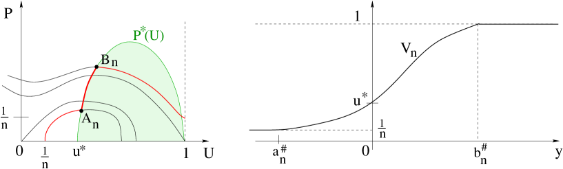
Figure 12: The construction of upper solutions. Left: a concatenation of a trajectory of (2.5) through $(n^{-1},0)$, followed by an arc along the curve where $P=P^{*}(U)$, followed by a trajectory of (2.5) through $(1,n^{-1})$. Right: the corresponding traveling profile in (7.20)-(7.21), shifted so that $V_{n}(0)=u^{*}$. By construction we have $V_{n}^{\prime}(a^{\prime}_{n})=0$, while $V_{n}^{\prime}(b^{\prime}_{n})>0$.

3. Toward the construction of upper solutions, consider again the 1-dimensional equation

$$u_{t}~{}=~{}f(u)+u_{xx}-u\,\alpha\,,$$ (7.18)

where $\alpha=\alpha(t,x)\geq 0$ is the control function. For a given wave speed $c>c^{*}$, a traveling profile $u(t,x)=U(x-ct)$ is an upper solution provided that

$$U^{\prime\prime}+cU^{\prime}+f(U)-\alpha\,U~{}\leq~{}0.$$ (7.19)

Assuming that $f$ satisfies (A2)-(A3), we consider the path $\gamma_{n}$ obtained by concatenating the following three curves (see Fig. 12, left)

• The trajectory of (2.5) starting at $(n^{-1},0)$, up to the point $A_{n}$ where it intersects the curve $P=P^{*}(U)\doteq\sqrt{Uf(U)}$.

• The trajectory of (2.5) ending at $(1,n^{-1})$, continued backward up to a point $B_{n}$ along the curve where $P=P^{*}(U)$.

• The portion of the curve $P=P^{*}(U)$ between $A_{n}$ and $B_{n}$.

As shown in Fig. 12, right, this yields a traveling profile for (7.18), say $u(t,x)=V_{n}(x-ct)$, which satisfies

$$V_{n}(0)=u^{*},\qquad\qquad V_{n}^{\prime\prime}+cV_{n}^{\prime}+f(V_{n})+V_{n}\alpha_{n}~{}=~{}0\quad\hbox{for}~{}~{}y\in[a^{\sharp}_{n},b^{\sharp}_{n}],$$ (7.20)

$$\left\{\begin{array}[]{rl}V_{n}(a^{\sharp}_{n})&=~{}{1\over n},\\[5.69054pt] V^{\prime}_{n}(a^{\sharp}_{n})&=~{}0,\end{array}\right.\qquad\left\{\begin{array}[]{rl}V_{n}(b^{\sharp}_{n})&=~{}1,\\[5.69054pt] V^{\prime}_{n}(b^{\sharp}_{n})&>~{}0,\end{array}\right.$$ (7.21)

for some values $a^{\sharp}_{n}<0<b^{\sharp}_{n}$ and a suitable control $\alpha_{n}\geq 0$. We can extend $V_{n}$ outside the interval $[a^{\sharp}_{n},b^{\sharp}_{n}]$ by setting

$$V_{n}(y)~{}=~{}\left\{\begin{array}[]{cl}{1\over n}&\hbox{if}\quad y\leq a^{\sharp}_{n}\,,\\[5.69054pt] 1&\hbox{if}\quad y\geq b^{\sharp}_{n}\,.\end{array}\right.$$ (7.22)

We remark that the above profiles $V_{n}$, as well as the interval $[a^{\sharp}_{n},b^{\sharp}_{n}]$, all depend on the wave speed $c$. To be reminded of this fact, we shall use the notations $V_{n}^{c}$, $a^{\sharp}_{n}(c)$, $b^{\sharp}_{n}(c)$.

In connection with (7.12) we observe that, as long as the speed $c\in[c_{2},c_{3}]$ remains in a bounded interval, also the intervals $\bigl{[}a^{\sharp}_{n}(c),b^{\sharp}_{n}(c)\bigr{]}$ remain uniformly bounded 4. Using the above traveling profiles $U_{n},V_{n}$, we are now ready to construct sequences of upper and lower solutions.

Choose a sequence $\varepsilon_{n}\downarrow 0$ such that, for every $n\geq 1$,

$${1\over\sqrt{\varepsilon_{n}}}~{}\geq~{}(b_{n}-a_{n})+\bigl{(}b^{\sharp}_{n}(c)-a^{\sharp}_{n}(c)\bigr{)}\quad\qquad\hbox{for all}~{}~{}c\in[c_{2},c_{3}].$$ (7.23)

Define the rescaled profiles

$$\widetilde{U}_{n}(y)~{}=~{}U_{n}\left(y-\sqrt{\varepsilon_{n}}\over\varepsilon_{n}\right),\qquad\qquad\widetilde{V}_{n}^{c}(y)~{}\doteq~{}V_{n}^{c}\left(y+\sqrt{\varepsilon_{n}}\over\varepsilon_{n}\right).$$ (7.24)

Notice that, by the definitions of $U_{n}$ and $V_{n}^{(c)}$, this implies

$$\widetilde{U}_{n}(y)~{}=~{}\left\{\begin{array}[]{cl}0&\hbox{if}~{}~{}y\leq 0,\\[2.84526pt] 1-n^{-1}&\hbox{if}~{}~{}y\geq 2\sqrt{\varepsilon_{n}}\,,\end{array}\right.\qquad\qquad\widetilde{V}^{c}_{n}(y)~{}=~{}\left\{\begin{array}[]{cl}n^{-1}&\hbox{if}~{}~{}y\leq-2\sqrt{\varepsilon_{n}},\\[2.84526pt] 1&\hbox{if}~{}~{}y\geq 0\,.\end{array}\right.$$ (7.25)

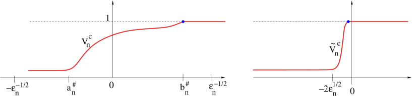
Figure 13: The traveling profile $V^{c}_{n}$, providing an upper solution, and its rescaled version $\widetilde{V}^{c}_{n}$ at (7.25).

Recalling the parameterization (7.3) of the boundary $\partial\Omega(t)$, consider the annular domain

$${\cal D}_{n}(t)~{}\doteq~{}\Big{\{}x(t,\xi)+y\,{\bf n}(t,\xi)\,;\quad\xi\in S,\quad|y|\leq 2\sqrt{\varepsilon_{n}}\Big{\}}.$$ (7.26)

Thanks to our earlier assumptions on the map $(t,\xi)\mapsto x(t,\xi)$, for all $\varepsilon_{n}>0$ small enough the map

$$(\xi,y)~{}\mapsto~{}x(t,\xi)+y\,{\bf n}(t,\xi)\qquad\qquad x(t,\xi)+y\,{\bf n}(t,\xi)$$

has a smooth inverse, for every $t\in[0,T]$.

We now define a lower solution $u^{-}_{n}$ by setting

$$u^{-}_{n}\Big{(}x(t,\xi)+y\,{\bf n}(t,\xi)\Big{)}~{}\doteq~{}\widetilde{U}_{n}(y)\qquad\qquad\hbox{for all}~{}~{}|y|\leq 2\sqrt{\varepsilon_{n}},$$ (7.27)

and extending $u_{n}^{-}$ outside the annulus ${\cal D}_{n}(t)$ as a constant function. Namely: $u_{n}^{-}(t,x)=0$ in the interior of $\Omega(t)$, while $u_{n}^{-}(t,x)=1-n^{-1}$ outside $\Omega(t)$. This is possible because of (7.25).

Similarly, we define an upper solution $u^{+}_{n}$ by setting

$$u^{+}_{n}\Big{(}x(t,\xi)+y\,{\bf n}(t,\xi)\Big{)}~{}\doteq~{}\widetilde{V}^{\beta(t,\xi)}_{n}(y),$$ (7.28)

and extending $u_{n}^{-}$ outside the annulus ${\cal D}_{n}(t)$ as a constant function. Namely: $u_{n}^{+}(t,x)=n^{-1}$ in the interior of $\Omega(t)$, while $u_{n}^{-}(t,x)=1$ outside $\Omega(t)$. Again, this is possible because of (7.25).

By construction, it is clear that $0\leq u^{-}_{n}(t,x)\leq u^{+}_{n}(t,x)\leq 1.$ Moreover,

$$u_{n}^{-}(t,\cdot)\to{\bf 1}_{\Omega(t)}\qquad\hbox{in}\qquad{\bf L}^{1}({\mathbb{R}}^{2}).$$

However, we only have

$$u_{n}^{+}(t,\cdot)\to{\bf 1}_{\Omega(t)}\qquad\hbox{in}\qquad{\bf L}^{1}_{loc}({\mathbb{R}}^{2}),$$

because $u_{n}^{+}(t,x)\geq n^{-1}$ and hence this upper solution is not integrable on ${\mathbb{R}}^{2}$.

To cope with this problem, observing that the minimum between two upper solutions is an upper solution, we can proceed as follows. Let $R>0$ be a radius large enough so that all sets $\Omega(t)$ remain inside the disc $B(0,R)\subset{\mathbb{R}}^{2}$. Consider the radially symmetric function

$$\phi(x)~{}\doteq~{}\begin{cases}1\quad&|x|\leq R,\\ e^{-|x|+R}\quad&|x|\geq R\end{cases}$$ (7.29)

Notice that, for $\varepsilon$ small enough, this is a time-independent upper solution of

$$u_{t}~{}=~{}\varepsilon\Delta u+{1\over\varepsilon}f(u),$$

integrable over the entire plane ${\mathbb{R}}^{2}$.

Replacing the functions $u_{n}^{+}$ with

$$v_{n}(t,x)~{}=~{}\min~{}\Big{\{}u_{n}^{+}(t,x),\,\phi(x)\Big{\}},$$

we obtain a new sequence of upper solutions. We claim that this sequence converges to ${\bf 1}_{\Omega(t)}$ in ${\bf L}^{1}({\mathbb{R}}^{2})$, for every $t\in[0,T]$. Indeed, for every $n\geq 1$ sufficiently large one has

$$\begin{array}[]{rl}\displaystyle\int_{{\mathbb{R}}^{2}}|v_{n}(t,x)-{\bf 1}_{\Omega(t)}|\,dx~{}=~{}\int_{B(0,R+\ln n)\setminus\Omega(t)}u^{+}_{n}(t,x)\,dx~{}+~{}\int_{|x|>R+\ln n}\phi(x)\,dx\\[11.38109pt] \displaystyle~{}\leq~{}\hbox{meas}({\cal D}_{n}(t)\setminus\Omega(t))+{\pi(R+\ln n)^{2}\over n}+\int_{|x|>R+\ln n}e^{-|x|+R}\,dx,\end{array}$$ (7.30)

and each term on the right hand side of (7.30) goes to zero as $n\to\infty$. 5. For each $n\geq 1$, we now consider the cost of a control which renders $v_{n}$ an upper solution. The smallest control function $\alpha$ that fulfils this requirement is

$$\alpha_{n}~{}\doteq~{}{\bigl{[}\varepsilon_{n}\Delta v_{n}+\varepsilon_{n}^{-1}f(v_{n})-(v_{n})_{t}\bigr{]}_{+}\over v_{n}}$$ (7.31)

By construction, we already know that $v_{n}$ satisfies

$$\varepsilon_{n}\,\Delta v_{n}+\varepsilon_{n}^{-1}f(v_{n})~{}\leq~{}0~{}=~{}(v_{n})_{t}\qquad\hbox{for}~{}~{}x\notin{\cal D}_{n}(t).$$

It thus remains to estimate the integral

$$\int_{{\cal D}_{n}(t)}\alpha_{n}(t,x)\,dx,$$ (7.32)

and show that it converges to the right hand side of (7.11). 6. Over the set ${\cal D}_{n}(t)$, we shall use the coordinates $(\xi,y)\in S\times[-2\sqrt{\varepsilon_{n}},\,2+\sqrt{\varepsilon_{n}}]$ corresponding to the point

$$x~{}=~{}x(t,\xi)+y\,{\bf n}(t,\xi)\,.$$ (7.33)

Computing the Laplacian of $v_{n}$ in terms of the coordinates $\xi,y$, and calling $r=r(t,\xi,y)$ is the local radius of curvature (which is uniformly positive throughout the domain), we find

$$\begin{array}[]{rl}\Delta_{x}v_{n}&\displaystyle=~{}(v_{n})_{yy}+{1\over r}(v_{n})_{y}+{(v_{n})_{\xi\xi}-x_{\xi\xi}\cdot(v_{n})_{\xi}\ \over|x_{\xi}|^{2}}\\[8.53581pt] &\displaystyle=~{}{1\over\varepsilon_{n}^{2}}\bigl{(}V_{n}^{\beta(t,\xi)}\bigr{)}^{\prime\prime}\left(y+\sqrt{\varepsilon_{n}}\over\varepsilon_{n}\right)+{\cal O}(1)\cdot{1\over\varepsilon_{n}}+{\cal O}(1)\,.\end{array}$$ (7.34)

On the other hand,

$$\begin{array}[]{rl}\partial_{t}v_{n}&\displaystyle=~{}-{\beta(t,\xi)\over\varepsilon_{n}}\bigl{(}V_{n}^{\beta(t,\xi)}\bigr{)}^{\prime}\left(y+\sqrt{\varepsilon_{n}}\over\varepsilon_{n}\right)+{\cal O}(1).\end{array}$$ (7.35)

Using (7.20), with the speed $c=\beta(t,\xi)$, one obtains

$$\bigl{(}V_{n}^{\beta(t,\xi)}\bigr{)}^{\prime\prime}+\beta(t,\xi)\bigl{(}V_{n}^{\beta(t,\xi)}\bigr{)}^{\prime}+f\bigl{(}V_{n}^{\beta(t,\xi)}\bigr{)}+V_{n}^{\beta(t,\xi)}\cdot\alpha_{n}~{}=~{}0.$$

Combining the above estimates, we obtain

$$\varepsilon_{n}\Delta_{x}v_{n}+{1\over\varepsilon}f(v_{n})-\partial_{t}v_{n}~{}=~{}{1\over\varepsilon_{n}}V_{n}^{\beta(t,\xi)}\cdot\alpha_{n}+{\cal O}(1),$$ (7.36)

where $\alpha_{n}$ is the optimal control on the portion of curve from $A_{n}$ to $B_{n}$ in Fig. 12. 7. We now integrate (7.36) over the entire domain ${\cal D}_{n}$. Computing the Jacobian determinant of the transformation (7.33), we obtain

$$dx_{1}dx_{2}~{}=~{}\bigl{|}x_{\xi}(\xi,y)\bigr{|}\cdot\varepsilon_{n}\,d\xi dy.$$

Therefore, at any given time $t\in[0,T]$, there holds

$$\begin{array}[]{rl}\displaystyle\int_{{\mathbb{R}}^{2}}\alpha_{n}\,dx&\displaystyle=~{}\int_{{\cal D}_{n}}{\bigl{[}\varepsilon_{n}\Delta v_{n}+\varepsilon_{n}^{-1}f(v_{n})-(v_{n})_{t}\bigr{]}_{+}\over v_{n}}\,dx\\[11.38109pt] &\displaystyle=~{}\int_{S\times[-2\sqrt{\varepsilon_{n}},~{}2\sqrt{\varepsilon_{n}}]}\left[{\alpha_{n}(\xi,y)\over\varepsilon_{n}}+{\cal O}(1)\right]\,\bigl{|}x_{\xi}(\xi,y)\bigr{|}\varepsilon_{n}\,d\xi dy\\[11.38109pt] &\displaystyle=~{}\int_{S}E\bigl{(}\beta(t,\xi)\bigr{)}|x_{\xi}(t,\xi)\bigr{|}\,d\xi+{\cal O}(1)\cdot\varepsilon_{n}\,.\end{array}$$ (7.37)

Taking the limit as $\varepsilon_{n}\to 0$, this yields (7.11). 8. Having constructed a sequence of lower solutions $u_{n}^{-}$ and of upper solutions $v_{n}$ which both converge to the characteristic function ${\bf 1}_{\Omega(t)}$, by a comparison argument we obtain a sequence of solutions to

$$u_{n,t}~{}=~{}{1\over\varepsilon_{n}}f(u_{n})+\varepsilon_{n}\,\Delta u_{n}-u_{n}\alpha_{n}\,,\qquad\qquad t\in[0,T],~{}x\in{\mathbb{R}}^{2},$$ (7.38)

with $u_{n}^{-}\leq u_{n}\leq v_{n}$. By (7.37), these solutions satisfy

$$\lim_{n\to\infty}\Big{\|}u_{n}(t,\cdot)-{\bf 1}_{\Omega(t)}\Big{\|}_{{\bf L}^{1}}\,=~{}0,\qquad\quad\lim_{n\to\infty}\int_{{\mathbb{R}}^{2}}\alpha_{n}(t,x)\,dx~{}=~{}\int_{S}E(\beta(t,\xi))\,\bigl{|}x_{\xi}(t,\xi)\bigr{|}\,d\xi.$$ (7.39)

This achieves the proof. MM     

Remark 7.1

We expect that an entirely similar result could be proved in the case where $g(u,\alpha)=\alpha$, and $f$ satisfies either (1.4) or (1.5). In this case, the optimal traveling profiles are the ones described in Theorem 3.1, while the formulas (7.9) and (7.8) should be replaced respectively by

$$u^{\varepsilon}_{t}~{}=~{}{1\over\varepsilon}f(u^{\varepsilon})+\varepsilon\,\Delta u^{\varepsilon}-\alpha^{\varepsilon}\,,\qquad\qquad{\cal F}_{\varepsilon}(u)~{}\doteq~{}\int_{0}^{T}\int[\varepsilon\Delta u+\varepsilon^{-1}f(u)-u_{t}]_{+}\,dx\,dt\,.$$

References

- [1] J. P. Aubin and A. Cellina, Differential Inclusions, Springer-Verlag, Berlin, 1984.
- [2] S. Aniţa, V. Capasso, and G. Dimitriu, Regional control for a spatially structured malaria model. Math. Meth. Appl. Sci. 42 (2019), 2909–2933.
- [3] S. Aniţa, V. Capasso, and A. M. Mosneagu, Global eradication for spatially structured populations by regional control. Discr. Cont. Dyn. Syst., Series B, 24 (2019), 2511–2533.
- [4] A. Braides, -convergence for beginners. Oxford University Press, Oxford, 2002.
- [5] U. Boscain and B. Piccoli, Optimal Syntheses for Control Systems on 2-D Manifolds, Springer, New York, 2004.
- [6] A. Bressan, Differential inclusions and the control of forest fires, J. Differential Equations (special volume in honor of A. Cellina and J. Yorke), 243 (2007), 179–207.
- [7] A. Bressan, M. T. Chiri, and N. Salehi, Optimal control problems for moving sets. To appear.
- [8] A. Bressan, G. Coclite, and W. Shen, A multi-dimensional optimal harvesting problem with measure valued solutions, SIAM J. Control Optim. 51 (2013), 1186–1202 .
- [9] A. Bressan, M. Mazzola, and K. T. Nguyen, Approximation of sweeping processes and controllability for a set valued evolution, SIAM J. Control Optim. 57 (2019), 2487–2514.
- [10] A.Bressan and F. Rampazzo, On differential systems with vector-valued impulsive controls, Boll. Un. Matematica Italiana 2-B, (1988), 641–656.
- [11] A. Bressan and D. Zhang, Control problems for a class of set valued evolutions, Set-Valued Var. Anal. 20 (2012), 581?601.
- [12] L. Cesari, Optimization Theory and Applications, Springer-Verlag, 1983.
- [13] G. M. Coclite and M. Garavello, A time dependent optimal harvesting problem with measure valued solutions, SIAM J. Control Optim. 55 (2017), 913–935.
- [14] G. M. Coclite, M. Garavello, and L. V. Spinolo, Optimal strategies for a time-dependent harvesting problem, Discrete Contin. Dyn. Syst. Ser. S, 11 (2018), 865–900.
- [15] R. M. Colombo and N. Pogodaev, On the control of moving sets: Positive and negative confinement results, SIAM J. Control Optim. 51 (2013), 380–401.
- [16] R. M. Colombo, T. Lorenz and N. Pogodaev, On the modeling of moving populations through set evolution equations. Discrete Contin. Dyn. Syst. 35 (2015), 73–98.
- [17] R. M. Colombo and E. Rossi, A modeling framework for biological pest control. Math. Biosci. Eng. 17 (2020), 1413–1427.
- [18] J. M. Coron, Control and Nonlinearity, American Mathematical Society, Boston, 2007.
- [19] H. O. Fattorini and T. Murphy, Optimal control problems for nonlinear parabolic boundary control systems: the Dirichlet boundary condition. Diff. Integral Equat. 7 (1994), 1367–1388.
- [20] P. C. Fife, Mathematical Aspects of Reacting and Diffusing Systems. Springer Lecture Notes in Biomathematics, Springer, 1979.
- [21] H. Hermes and G. Haynes, On the nonlinear control problem with control appearing linearly. SIAM J. Control 1 (1963), 85–108.
- [22] I. Lasiecka, and R. Triggiani, Control theory for partial differential equations: continuous and approximation theories. I. Abstract parabolic systems. Encyclopedia of Mathematics and its Applications, 74. Cambridge University Press, Cambridge, 2000.
- [23] S. M. Lenhart and J. A. Montero, Optimal control of harvesting in a parabolic system modeling two subpopulations, Math. Models Methods Appl. Sci., 11 (2001), 1129–1141.
- [24] B. Miller and E. Rubinovich, Impulsive Control in Continuous and Discrete-Continuous Systems. Kluwer Academic/Plenum Publishers, New York, 2003.
- [25] R. W. Rishel, An extended Pontryagin maximum principle for control systems whose control laws contain measures, SIAM J. Control 3 (1965), 191–205.
- [26] D. Ruiz-Balet and E. Zuazua, Control under constraints for multi-dimensional reaction-diffusion monostable and bistable equations. J. Math. Pures Appl. 143 (2020) 345–375.
- [27] L. Seirin, R. Baker, E. Gaffney, and S. White, Optimal barrier zones for stopping the invasion of Aedes aegypti mosquitoes via transgenic or sterile insect techniques. Theoretical Ecology 6 (2013) 427–442.