A Sample of Massive Black Holes in Dwarf Galaxies Detected via [Fe X] Coronal Line Emission: Active Galactic Nuclei and/or Tidal Disruption Events

Abstract

The massive black hole (BH) population in dwarf galaxies ($M_{\rm BH}\lesssim 10^{5}~{}M_{\odot}$) can provide strong constraints on the origin of BH seeds. However, traditional optical searches for active galactic nuclei (AGNs) only reliably detect high-accretion, relatively high-mass BHs in dwarf galaxies with low amounts of star formation, leaving a large portion of the overall BH population in dwarf galaxies relatively unexplored. Here, we present a sample of 81 dwarf galaxies ($M_{\star}\leq 3\times 10^{9}~{}M_{\odot}$) with detectable [Fe X]$\lambda$6374 coronal line emission indicative of accretion onto massive BHs, only two of which were previously identified as optical AGNs. We analyze optical spectroscopy from the Sloan Digital Sky Survey and find [Fe X]$\lambda$6374 luminosities in the range $L_{[Fe\textsc{x}]}\approx 10^{36}$–$10^{39}$ erg s^-1, with a median value of $1.6\times 10^{38}$ erg s^-1. The [Fe X]$\lambda$6374 luminosities are generally much too high to be produced by stellar sources, including luminous Type IIn supernovae (SNe). Moreover, based on known SNe rates, we expect at most 8 Type IIn SNe in our sample. On the other hand, the [Fe X]$\lambda$6374 luminosities are consistent with accretion onto massive BHs from AGNs or tidal disruption events (TDEs). We find additional indicators of BH accretion in some cases using other emission line diagnostics, optical variability, X-ray and radio emission (or some combination of these). However, many of the galaxies in our sample only have evidence for a massive BH based on their [Fe X]$\lambda$6374 luminosities. This work highlights the power of coronal line emission to find BHs in dwarf galaxies missed by other selection techniques and to probe the BH population in bluer, lower mass dwarf galaxies.

1 Introduction

Supermassive black holes (BHs) are known to live in the nuclei of almost all massive galaxies (e.g., Kormendy & Richstone, 1995; Kormendy & Ho, 2013), but merger-driven galaxy growth has effectively erased their initial formation conditions (Volonteri, 2010; Natarajan, 2014). There are several proposed theories for the formation of the intial BH “seeds” in the early Universe, including remnants from Population III stars (Bromm & Yoshida, 2011), the direct collapse of gas clouds (Loeb & Rasio, 1994; Begelman et al., 2006; Lodato & Natarajan, 2006; Choi et al., 2015) and stellar collisions in dense star clusters (Portegies Zwart et al., 2004; Devecchi & Volonteri, 2009; Davies et al., 2011; Lupi et al., 2014; Stone et al., 2017). Each of these processes creates different size BH seeds; the remnants of Population III stars would create $M_{\rm BH}\sim 100~{}M_{\odot}$ (Bond et al., 1984; Heger & Woosley, 2002), while direct collapse and star cluster collisions would create $M_{\rm BH}\sim 10^{3}$–$10^{5}~{}M_{\odot}$.

While it is not feasible to observe the first BH seeds at high redshift, nearby dwarf galaxies can place strong constraints on their properties (see Reines & Comastri, 2016; Greene et al., 2020, and references therein). Dwarf galaxies have relatively quiet merger histories compared to their more massive counterparts (Bellovary et al., 2011), and may experience strong supernova feedback that stunts BH growth (Anglés-Alcázar et al., 2017; Habouzit et al., 2017). Therefore, if a dwarf galaxy does harbor a BH, it should have a mass relatively close to the initial seed mass (e.g., $M_{\rm BH}\lesssim 10^{5}$).

Unfortunately, the smaller masses and lower luminosities of BHs in dwarf galaxies make them difficult to detect. In the optical regime, narrow-line ratios consistent with active galactic nuclei (AGN) photoionization as well as broad H$\alpha$ emission have been used to identify BHs in dwarf galaxies (e.g., Reines et al., 2013; Baldassare et al., 2016). These studies incorporated the commonly used Baldwin, Phillips and Terlevich diagrams, (BPT diagrams; Baldwin et al., 1981) also referred to as the Veilleux & Osterbrock (1987, VO87) diagrams which use narrow-line ratios to differentiate between the spectral energy distributions of star forming regions and AGNs. However, these diagrams struggle with low-luminosity AGNs (LLAGNs), low ionization nuclear emission regions (LINERs) and contributions from shocks (see Ho, 2008; Kewley et al., 2019, for a review). Therefore, these studies often only detect the brightest, highest-accretion rate objects, leaving a large portion of the lower-mass, lower-accretion rate BHs relatively unexplored (Greene et al., 2020). Additionally, optical AGN indicators may be diluted by emission from the host galaxy, even in objects with low star-formation rates (SFRs; Moran et al., 2002; Groves et al., 2006; Stasińska et al., 2006; Cann et al., 2019). Any combination of these factors can easily hide AGN activity in optical surveys.

Infrared (IR) colors have also been used to identify AGNs in massive galaxies (Jarrett et al., 2011; Mateos et al., 2012; Stern et al., 2012), but is often confused with star formation in dwarf galaxies (Hainline et al., 2016; Condon et al., 2019; Latimer et al., 2021). Hard X-ray emission is a clean diagnostic when searching for AGN activity at high luminosities, but can be confused with high-mass X-ray binaries at low luminosities and can also miss obscured AGNs (Hickox & Alexander, 2018; Latimer et al., 2021). Similarly, radio emission is not affected by reddening due to dust and is produced by almost all AGNs (see Ho, 2008, and references therein), but the expected radio emission from BHs in dwarf galaxies could be similar to that from H II regions, supernova remnants or supernovae (e.g., Reines et al., 2008; Chomiuk & Wilcots, 2009; Johnson et al., 2009; Aversa et al., 2011; Kepley et al., 2014; Varenius et al., 2019; Reines et al., 2020). Therefore, it is challenging to find low accretion-rate, low-mass BHs using these detection methods.

Recently, Molina et al. (2021) and Kimbro et al. (2021) confirmed the presence of low-accretion rate BHs in the dwarf galaxies SDSS J122011.26+302008.1 (J1220+3020; ID 82 in Reines et al., 2020) and Mrk 709 S (Reines et al., 2014), respectively. Interestingly, both objects had clear detections of the coronal line [Fe X]$\lambda$6374. Due to its high ionization potential (262.1 eV; Oetken, 1977), [Fe X]$\lambda$6374 and other coronal lines are considered to be a reliable signature of AGN activity in galaxies (e.g., Penston et al., 1984; Prieto & Viegas, 2000; Prieto et al., 2002; Reunanen et al., 2003). While coronal-line emission is often considered to be produced by gas photoionized by the hard AGN continuum (e.g., Nussbaumer & Osterbrock, 1970; Korista & Ferland, 1989; Oliva et al., 1994; Pier & Voit, 1995), [Fe X]$\lambda$6374 emission can also be mechanically excited by radiative shock waves that are driven into the host galaxy by radio jets from the AGN (Wilson & Raymond, 1999). As both BHs studied in Molina et al. (2021) and Kimbro et al. (2021) had low accretion rates and strong radio detections, they conclude that the coronal-line emission is created mechanically by jet-driven winds. Given the presence of [Fe X]$\lambda$6374 emission in two different objects, one of which was detected in the Sloan Digital Sky Survey (SDSS) 3″ single-fiber spectrum, this discovery opens a new method for detecting low accretion-rate BHs in dwarf galaxies.

In this work we present the first systematic search for [Fe X]$\lambda$6374-selected massive BHs in dwarf galaxies, making use of SDSS 3″ single-fiber spectra. We describe our sample selection in Section 2. We then use various data sets to search for additional AGN markers in our sample. The analysis of the SDSS optical spectra, including several emission-line ratio diagnostics, are presented in Section 3. We then search for AGN-like optical variability in Section 4. Finally, we use archival Chandra data and radio surveys to search for X-ray and radio emission consistent with AGN activity in Sections 5 and 6. We discuss our results in Section 7 and summarize our findings in Section 8. In this paper, we assume a $\Lambda\textrm{CDM}$ cosmology with $\Omega_{\rm m}=0.3$, $\Omega_{\Lambda}=0.7$ and H${}_{0}=73$ km s^-1 Mpc^-1.

2 Dwarf Galaxies with [Fe X]$\lambda$6374 Emission

2.1 Sample Selection and Measurements

We selected our sample of dwarf galaxies from version v1_0_1 of the NASA-Sloan Atlas (NSA; Blanton et al., 2011). This updated version of the NSA was used to create the galaxy sample for the SDSS-IV Mapping Nearby Galaxies at Apache Point Observatory (MaNGA; Bundy et al., 2015; Yan et al., 2016; Blanton et al., 2017) survey, and is publicly available via the SDSS Data Release 16 (DR16; Ahumada et al., 2020). We note that any reference to NSA IDs in this paper use those from the v1_0_1 catalog. In this work, we used the single-fiber SDSS spectra to identify our sample of dwarf galaxies with [Fe X] emission. The spectra were taken with the 2.5-meter wide-field Sloan Foundation Telescope and the 640-fiber double spectrograph at Apache Point Observatory, New Mexico (Gunn et al., 2006). The fibers are 3″ in diameter, cover a wavelength range of 3800–9200 Å, and have an instrumental dispersion of 69 km s^-1 per pixel. All spectra in DR16 were processed using the version v5_13_0 of the idlspec2d pipeline (Bolton et al., 2012; Dawson et al., 2013), which performs both the data reduction and emission-line measurements.

As we are interested in limiting our search to dwarf galaxies, we use the same mass constraint as Reines et al. (2013), i.e., $M_{*}\leq 3\times 10^{9}~{}{\rm M}_{\odot}$, and require that each galaxy has a single-fiber SDSS spectrum. We identify 46,530 objects that meet these criteria. While we relied on the NSA to identify our parent sample of dwarf galaxies, we wrote our own software to search for and measure the [Fe X]$\lambda$6374 line.

After we defined our parent sample of dwarf galaxies, we identified all galaxies with [Fe X] emission. Previous work on [Fe X]-emitting dwarf galaxies by Molina et al. (2021) and Kimbro et al. (2021) demonstrated that the [Fe X] emission will be both relatively weak, even compared to the [O I] doublet, and well-described by a single Gaussian. Additionally, Molina et al. (2021) found that the [Fe X] emission in J1220+3020 was confined to the central 1″ using Gemini IFU spectroscopy. We therefore expect weak [Fe X]$\lambda$6374 emission in the much larger 3″ aperture that may not exhibit the typical asymmetric profiles seen in AGNs in more massive galaxies (e.g., Gelbord et al., 2009). In order to account for both of these issues, we created a pipeline that fits both the [O I] doublet and any potential, weak [Fe X]$\lambda$6374 emission. Our processing pipeline utilizes the python packages astropy (Astropy Collaboration et al., 2013, 2018), matplotlib (Hunter, 2007) and pyspeckit (Ginsburg & Mirocha, 2011), which is a program that wraps around the python package MPFIT and is customized to fit astronomical spectra.

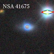
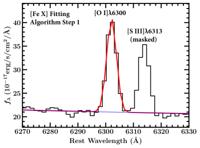
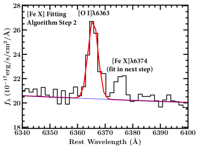
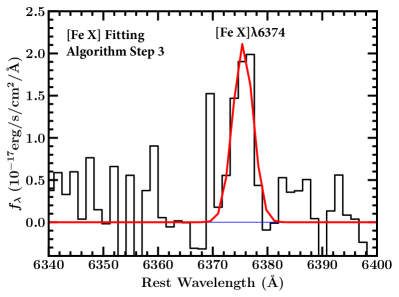
Figure 1: Top Left: The DESI Legacy Imaging Survey SkyViewer $grz$ image of the [Fe X]-emitting dwarf galaxy NSA 41675. The position of the galaxy nucleus as defined by the NSA is shown as the red cross, and the spatial extent of the SDSS 3″ fiber is shown as the the red circle. Top Right: The fit of the [O III]$\lambda$6300 line in NSA 41675, and first step in the [Fe X] fitting algorithm. The data are in black, the model is shown as the solid red line, and the baseline is shown as the solid blue line. The [S III]$\lambda$6313 line is detected and masked in this fit. Bottom left: The second step in the [Fe X] fitting algorithm, with the data shown as a solid black line. In this step the [O III]$\lambda$6363 emission-line model is precisely defined by the fitted [O III]$\lambda$6300 line. The [O III]$\lambda$6363 emission line and baseline fit (blue solid line) are added together to create the total model shown as the red line. The total model is subtracted to create the residual spectrum with the [Fe X] line. Bottom Right: Fit to the [Fe X]$\lambda$6374 emission line in the residual spectrum after subtracting the [O I] emission and continuum. The data are in black, the model is over-plotted in red, and the “continuum” baseline is shown in blue. We show the galaxy and the fitted [Fe X] emission line for all 81 dwarf galaxies in the Appendix.

We first required that the stronger line in the [O I] doublet, [O I]$\lambda$6300, was detected with a signal-to-noise (S/N) $\geq$ 3 in the automated SDSS spectroscopy pipeline, idlspec2d. This S/N check is important for two reasons: (1) strong [O I] emission was seen in the two previous AGN candidates with [Fe X]$\lambda$6374 emission and is generally associated with AGN activity (Kewley et al., 2006; Reines et al., 2020; Molina et al., 2021; Kimbro et al., 2021), and (2) a strong [O I]$\lambda$6300 detection will ensure a clean subtraction of the weaker line in the doublet, [O I]$\lambda$6363 which could be blended with the [Fe X]$\lambda$6374 emission.

If this criterion is met, we then fit the [O I]$\lambda$6300 line using pyspeckit. We simultaneously fit a second-order polynomial to describe the continuum around the [O I]+[Fe X] complex (spanning $\sim 150$Å) and a single Gaussian to describe [O I]$\lambda$6300. We mask the emission line [S III]$\lambda$6313 if present to ensure a good fit to the continuum. In all cases, the [O I]$\lambda$6300 and [S III]$\lambda$6313 emission lines were not blended. We repeat the fitting process using a 2-Gaussian model, and select the 2-Gaussian model if it results in a reduced $\chi^{2}$ that is 10% smaller than the 1-Gaussian model. An example of an [O I]$\lambda$6300 fit is shown in the top right panel of Figure 1.

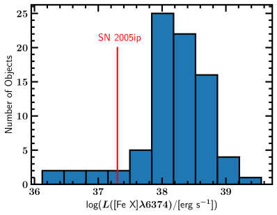
Figure 2: The distribution of [Fe X]$\lambda$6374 luminosities in our sample. The red line denotes the [Fe X] luminosity of the type IIn supernova SN 2005ip at its most luminous state at $\sim$100 days post-explosion. A majority of our objects fall well above that line, indicating that a single type IIn supernova cannot explain the observed emission. See Section 7.1 for a more in-depth discussion.

We use the [O I]$\lambda$6300 line as a template to perfectly describe the [O I]$\lambda$6363 line. Specifically, we shift the model according to their rest wavelengths of 6365.536 and 6302.046, respectively, constrain the widths to be the same in velocity, and require a flux ratio of [O I]$\lambda$6300/[O I]$\lambda 6363=3$. For the 2-Gaussian models, we also require that the relative position and height ratios are the same for the [O I]$\lambda 6363$ model. We then fit the continuum around the [O I]+[Fe X] complex ($\sim 150$Å) with a second-order polynomial and subtract both the continuum fit and the [O I]$\lambda 6363$ model. This process leaves a residual spectrum, with a potential [Fe X]$\lambda$6374 line. An example of an [O I]$\lambda$6363 fit is shown in the bottom left panel of Figure 1.

We then fit a single Gaussian to the residual spectrum to model the [Fe X]$\lambda$6374 emission line and measure the root mean square (rms) of the two continuum windows on either side of [Fe X], which are each approximately $50$Å wide. This measurement represents the $\sigma$, or noise in the residual spectrum. We accept the fit if the full-width at half maximum (FWHM) of the Gaussian is greater than or equal to the instrumental resolution at the observed wavelength of the [Fe X]$\lambda$6374 line, the peak of the Gaussian is at least 2$\sigma$ above the noise in the residual spectrum and the integrated flux has a ${\rm S/N}\geq 2$. Using these criteria, the pipeline identified 213 galaxies with detected [Fe X] emission. In all cases, a single Gaussian best describes the observed [Fe X] emission, and the residuals are consistent with the surrounding noise.

The automated pipeline described above was purposely inclusive as [Fe X] is predicted to be a weak line. We therefore expected some of the flagged objects to be “false positives”, such that the “detected” [Fe X] emission is actually noise. We visually inspected all of the fits and removed a total of 130 objects that appeared to be false positives. 70 out of the 130 rejected [Fe X] Gaussian fits were driven by one or two pixels, while the remaining 60 were very broad fits to noise. After that cut, we then removed 2 additional galaxies from the sample that were directly behind larger, foreground galaxies. Our final sample consists of 81 objects. Figure 1 shows an example of an accepted [Fe X]$\lambda$6374 fit, along with the image of the host galaxy from the Dark Energy Spectroscopic Instrument (DESI) Legacy Imaging Survey (Dey et al., 2019). The rest of the [Fe X] emission line and galaxy pairs are shown in Appendix A. We note that some of the [Fe X] profiles do appear somewhat asymmetric similar to that seen in previous coronal-line studies (e.g., Gelbord et al., 2009), but given their low S/N we do not attempt to characterize their profiles. The 81 dwarf galaxies in our final sample have a range of [Fe X]$\lambda$6374 luminosities given by $L_{[Fe\textsc{x}]}\approx 10^{36}$–$10^{39}$ erg s^-1, and a median value of $1.6\times 10^{38}$ erg s^-1. We show the distribution of the [Fe X] luminosities in Figure 2.

We find that all of the SDSS spectra are within 3″ of the galaxy nucleus as defined by the NSA, and only 4 spectra have centroids farther than 1$\farcs$5 away from the galactic center. We list the relative distance between the spectroscopic fiber and the galaxy center and the basic properties of the host galaxy in Table 1. The [Fe X] line measurements are listed in Table 2. Notes on individual objects, such as their inclusion in previous studies, are also given in the Appendix.

=0.5in

Table 1: Sample of 81 [Fe X]$\lambda$6374-emitting Dwarf Galaxies

Galaxy Properties										Previous Studies
NSAID	RAGal	DECGal	RASpec	DECSpec	$\Delta$Spec	$z$	$\log(M_{*}/M_{\odot})$	SFR	12+log([O/H])	Reference	Class.
(1)	(2)	(3)	(4)	(5)	(6)	(7)	(8)	(9)	(10)	(11)	(12)
50	146.00780	-0.64226	146.00779	-0.64227	0.05	0.00478	7.8	0.17	7.7	Reines+20	SF
6055	173.70484	-1.06324	173.70481	-1.06331	0.27	0.04641	9.5	0.40	8.5	BGG20	AGN
10870	199.48543	1.11862	199.48541	1.11860	0.1	0.03106	9.4	0.40	8.5
15288	225.98677	-0.70008	225.98675	-0.70007	0.08	0.14134	9.4	6.13	8.2
21569	199.19674	-3.04933	199.19659	-3.04942	0.63	0.01876	9.1	0.10	8.3
30143	343.15207	-0.55478	343.15162	-0.55493	1.71	0.0543	9.1	0.95	8.3
41675	8.07754	15.00393	8.07747	15.00394	0.25	0.01787	8.2	0.51	8.1
46653	118.01749	42.75672	118.01755	42.75673	0.16	0.04113	9.3	0.38	8.5
50800	131.36501	53.14802	131.36507	53.14805	0.17	0.03107	8.5	1.59	8.1
61382	177.82335	67.31233	177.82341	67.31234	0.09	0.04599	9.4	0.45	8.3
61601	175.77729	68.12157	175.77723	68.12160	0.13	0.04892	8.9	1.88	8.2
63560	211.73123	65.91572	211.73115	65.91572	0.12	0.05995	9.4	3.15	8.4
95985	234.26741	55.26406	234.26740	55.26406	0.02	0.00225	7.5	0.03	8.1	BWA20	AGN
102990	316.78814	-7.42285	316.78811	-7.42287	0.13	0.02830	8.8	0.17	8.4
107232	9.14935	-10.05103	9.14942	-10.05099	0.29	0.02080	9.5	0.38	8.6
108471	12.84411	-11.14529	12.84402	-11.14531	0.33	0.02085	9.0	0.20	8.4
115843	53.95511	-0.65364	53.95512	-0.65364	0.04	0.03067	8.9	0.17	8.4
131809	140.10780	50.82773	140.10764	50.82762	0.54	0.03444	9.2	0.24	8.5	BGG20	AGN
140290	47.31564	-0.94906	47.31566	-0.94902	0.16	0.05718	8.8	0.59	8.2
140756	49.07568	1.00611	49.07570	1.00607	0.16	0.03311	8.7	0.31	8.3
141378	52.61371	-0.85374	52.61371	-0.85377	0.11	0.05243	9.3	0.57	8.5
141686	47.26619	0.64633	47.26618	0.64630	0.11	0.03009	8.1	0.21	7.9
144266	253.94519	36.67987	253.94519	36.67990	0.11	0.06234	9.0	1.21	8.2
162936	126.20782	38.58743	126.20768	38.58737	0.45	0.03041	8.8	0.16	8.5
164449	137.39846	45.95532	137.39844	45.95529	0.12	0.02733	8.8	0.13	8.5
174326	127.60643	33.05816	127.60641	33.05816	0.06	0.02086	9.1	0.19	8.5
201943	314.23197	-0.40761	314.23196	-0.40758	0.11	0.02946	8.7		8.3
213780	53.97134	-0.66295	53.97135	-0.66295	0.04	0.03016	8.8	0.21	8.4
220716	229.68660	51.20768	229.68655	51.20773	0.21	0.01418	8.8	0.05	8.3
237974	180.71961	10.24299	180.71954	10.24300	0.25	0.06167	9.4	0.87	8.4
256515	185.24312	56.35518	185.24313	56.35515	0.11	0.03461	9.5	0.38	8.6
256802	185.92845	58.24618	185.92837	58.24615	0.19	0.01437	9.4	0.14	8.4	Reines+13	AGN
258576	201.97411	55.64514	201.97408	55.64516	0.09	0.03845	8.9	0.38	8.4
270622	162.36197	42.24777	162.36176	42.24761	0.80	0.02410	8.2	0.06	8.4
275961	207.85572	40.21324	207.85573	40.21327	0.11	0.00823	9.4	0.25	8.6	Reines+13	Compos
ite 282978	230.02922	37.99824	230.02922	37.99821	0.11	0.06432	9.5	0.75	8.5
300542	198.27999	46.09894	198.27964	46.09844	2.00	0.02965	9.3	0.12	8.4	Reines+13	Sne
305229	19.43879	-1.17564	19.43877	-1.17558	0.23	0.10881	8.9	1.87	8.1
321197	160.50153	12.33491	160.50154	12.33493	0.08	0.00257	8.1	0.01	8.3
328894	180.55578	6.28306	180.55576	6.28311	0.19	0.03634	8.7	0.34	8.5
331005	189.78945	8.14025	189.78975	8.13952	2.84	0.04948	8.9	0.44	8.5
331627	213.86196	36.40828	213.86185	36.40825	0.34	0.02817	9.4	0.52	8.5
345375	191.88671	13.61817	191.88671	13.61815	0.07	0.08469	9.2	1.16	8.5
366027	133.68095	8.94791	133.68087	8.94795	0.32	0.02962	9.1	0.32	8.1
393631	214.09711	33.12361	214.09713	33.12359	0.09	0.08324	9.4	2.88	8.5
401495	123.37373	54.74468	123.37383	54.74482	0.55	0.03234	8.7	0.27	8.4
402252	125.55366	58.02834	125.55370	58.02836	0.10	0.01645	8.3	0.06	8.2
409020	137.05685	26.70089	137.05690	26.70085	0.22	0.07682	9.2	3.02	8.2
418928	169.03563	30.37582	169.03562	30.37583	0.05	0.04164	9.4	0.25	8.6
421523	192.17151	38.57556	192.17129	38.57556	0.62	0.04121	9.4	0.27	8.6
422297	185.79998	37.99107	185.79997	37.99108	0.05	0.00752	7.8	0.01	8.2
426303	162.33047	37.87624	162.33031	37.87614	0.58	0.02526	9.2	0.18	8.4
426824	176.12647	32.56818	176.12646	32.56815	0.11	0.03072	8.7	0.30	8.3
427201	199.01634	29.38181	199.01632	29.38169	0.44	0.03779	9.1	4.92	8.3	Reines+13	SF+BHa
437653	198.02611	39.15767	198.02636	39.15771	0.71	0.02147	9.2	0.16	8.5
442120	204.73782	36.59586	204.73785	36.59584	0.11	0.01940	8.8	0.09	8.3
442212	203.50222	36.70000	203.50220	36.70002	0.09	0.05988	8.6	1.43	8.0
442427	201.58173	36.86264	201.58171	36.86266	0.09	0.05588	9.4	0.91	8.5
452253	216.75820	28.25949	216.75819	28.25950	0.05	0.04027	9.3	0.27	8.5
452914	216.15493	26.34413	216.15507	26.34419	0.50	0.03539	9.2	0.12	8.6
457940	224.50743	26.22497	224.50738	26.22500	0.19	0.03552	9.2	0.38	8.5
458829	161.33505	9.39698	161.33508	9.39697	0.11	0.05487	9.1	7.54	8.2
472272	245.46907	15.31555	245.46905	15.31555	0.07	0.03434	8.7	2.92	8.3
472333	246.57067	16.32011	246.57065	16.32012	0.08	0.01295	9.1	0.07	8.5
473078	167.42962	25.63336	167.42962	25.63335	0.04	0.04121	9.4	0.30	8.6
491412	139.91023	19.59117	139.91025	19.59119	0.10	0.05696	9.1	2.10	8.2
501341	157.95713	23.41739	157.95712	23.41741	0.08	0.00408	7.8	0.03	8.1
524413	178.57025	24.97274	178.57023	24.97274	0.07	0.02866	9.2	0.20	8.5
525522	237.71971	15.73100	237.71970	15.73099	0.05	0.03506	9.2	0.25	8.4
532026	138.83771	12.43752	138.83769	12.43755	0.13	0.03330	9.1	0.47	8.4
533731	147.32514	16.87894	147.32513	16.87896	0.08	0.05199	9.7	7.18	8.4	Kimbro+21	AGN
536931	157.45538	16.18098	157.45535	16.18091	0.27	0.01089	9.0	0.18	8.3
541112	202.54870	16.65336	202.54873	16.65332	0.18	0.03016	9.0	0.27	8.3
553772	208.69741	15.50116	208.69740	15.50120	0.15	0.02404	9.2	0.20	8.5
557918	206.56320	17.91621	206.56323	17.91624	0.15	0.02571	9.3	0.25	8.4
571629	231.46649	17.70089	231.46631	17.70061	1.18	0.02922	9.3	0.18	8.5
577169	129.78605	33.30856	129.78601	33.30857	0.13	0.05438	9.1	1.23	8.3
625882	166.28381	44.74638	166.28383	44.74646	0.29	0.02154	9.3	5.11	8.2
632355	225.98191	0.43211	225.98190	0.43214	0.11	0.00529	7.8	0.04	8.0
656364	163.93653	46.37194	163.93590	46.37180	1.64	0.05065	8.5	0.74	8.4
670127	191.12724	40.73691	191.12728	40.73690	0.11	0.01790	9.3	1.29	8.4

Note. — Column (1): The NSA IDs from version v1_0_1 of the NSA Catalog. Columns (2)–(5): The RA and DEC values in degrees of the galaxy center (denoted with Gal) and the spectroscopic SDSS fiber (denoted with Spec). Column (6): The offset between the spectroscopic fiber and the galaxy center in arcseconds. Columns (7) – (8): The redshift and stellar mass (in units of solar masses) from the NSA, assuming $h=0.73$. Column (9): The total star formation rate in units of $M_{\odot}$ yr^-1 calculated from the GALEX FUV and WISE W4 measurements as described in Section 2.2. Column (10): Metallicity calculated via Pettini & Pagel (2004), assuming the [N II] and H$\alpha$ flux measurements that are measured directly from the SDSS 3″ spectra in this work. The emission-line flux measurements are presented in Table 3. Column (11): The inclusion of this object in previous studies; Reines+13 refers to Reines et al. (2013), BGG20 refers to Baldassare et al. (2020), BWA20 refers to Birchall et al. (2020), Reines+20 refers to Reines et al. (2020) and Kimbro+21 refers to Kimbro et al. (2021). Column (12) provides the designation of the object from previous studies.

Table 2: [Fe X]$\lambda$6374 Measurements

NSAID	$f$([Fe X])	log($L_{\rm[FeX]}$)	$\sigma_{\rm peak}$	$S/N_{\rm line}$	$L$([Fe X])${}_{\rm gal}/L$([Fe X])SN2005ip
(1)	(2)	(3)	(4)	(5)	(6)
50	$11.7\pm 3.8$	$36.7\pm 0.5$	3.1	3.1	0.3
6055	$6.1\pm 3.0$	$38.4\pm 0.3$	2.1	2.0	12.2
10870	$10.2\pm 4.6$	$38.3\pm 0.4$	2.3	2.2	9.2
15288	$8.9\pm 4.3$	$39.6\pm 0.3$	3.2	2.1	165.4
21569	$8.6\pm 4.3$	$37.8\pm 0.3$	2.9	2.0	2.8
30143	$11.5\pm 4.4$	$38.8\pm 0.4$	2.2	2.6	31.6
41675	$9.8\pm 4.0$	$37.8\pm 0.4$	3.9	2.5	2.9
46653	$4.0\pm 2.0$	$38.1\pm 0.3$	3.6	2.0	6.3
50800	$8.2\pm 3.8$	$38.2\pm 0.3$	2.3	2.2	7.4
61382	$4.2\pm 1.9$	$38.3\pm 0.4$	4.2	2.2	8.3

Note. — The entirety of Table 2 is published in the electronic edition of The Astrophysical Journal. We show a portion here to give information on its form and content. Column (1): NSA identification number. Column (2): The measured [Fe X]$\lambda$6374 flux in units of $10^{-17}$ erg s^-1 cm^-2. Column (3): The measured [Fe X]$\lambda$6374 luminosity in units of erg s^-1. Column (4): The strength of the line peak in units of the residual spectrum noise, $\sigma$. Column (5): The S/N of the integrated line flux. Column (6): The ratio of the measured [Fe X]$\lambda$6374 luminosity from column (3) to the peak [Fe X]$\lambda$6374 lumionsity in SN2005ip, $\sim 2\times 10^{37}$ erg s^-1.

2.2 Properties of the Host Galaxies

The [Fe X]$\lambda$6374-emitting dwarf galaxies span a mass range of $7.5\leq\log(M_{*}/M_{\odot})\leq 9.5$, with a median mass of $\log(M_{*}/M_{\odot})=9.1$. All reported masses are from the NSA except for Mrk 709S (NSA 533731), which is taken from Reines et al. (2014). The stellar mass for Mrk 709S from Reines et al. (2014) is estimated to be $\log(M_{*}/M_{\odot})=9.4$, which is derived using photometry that separates the northern and southern galaxies in the pair. The NSA automated pipeline value is $\log(M_{*}/M_{\odot})=9.7$ which is likely higher due to additional light from the other components in the system. The galaxies span a redshift range of $0.00225\leq z\leq 0.14134$, with a median $z=0.03107$. All of our objects are relatively nearby; only two objects have $z>0.1$, while 76% of the galaxies have $z<0.05$. The distribution of the galaxy redshifts in our sample is shown in Figure 3.

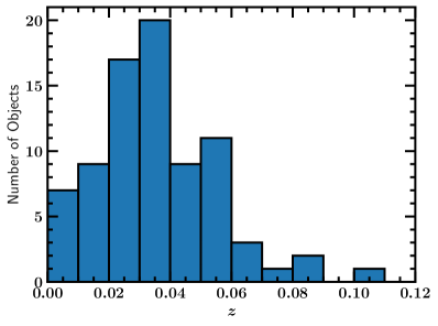
Figure 3: The distribution of the host galaxy redshifts in our sample. Only two objects have $z>0.1$, and 76% have $z<0.05$.

The galaxies in our sample vary in size, with $r$-band half-light radii ranging from $\sim$0.7″–16.2″ (0.1–16.3 kpc) with a median value of 3.6″ (2.1 kpc). While 11 objects in our sample were classified as spiral galaxies by Galaxy Zoo 1 (Lintott et al., 2011), a majority appear irregular in morphology. One interesting feature of this sample is how blue, and thus vigorously star-forming, a majority of the galaxies are, as clearly seen in the Legacy Survey images in the Appendix. In fact, the median $g-r$ color is 0.37, and spans the range $-0.42\leq g-r\leq 0.68$. We show the $g-r$ vs. $M_{*}$ diagram in Figure 4.

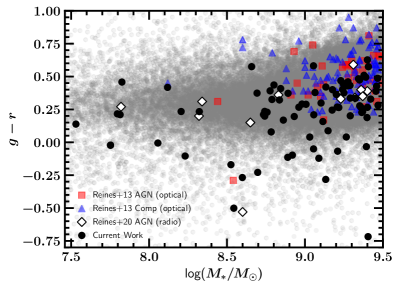
Figure 4: The $g-r$ vs. stellar mass plot. The [Fe X]$\lambda$6374-emitting AGN candidates from this work are shown in black circles, the optically-selected AGN and composite objects from Reines et al. (2013) are shown as red squares and blue triangles, respectively and the radio-selected AGNs from Reines et al. (2020) are shown as unfilled white diamonds. These four samples are plotted over the distribution of dwarf galaxies from the NSA. The Reines et al. (2013) optically-selected sample tends to have higher-mass, redder host galaxies, while the Reines et al. (2020) radio-selected sample and the [Fe X]-selected galaxies in this work tend to trace a lower-mass, bluer population.

We quantified the global star formation rates (SFRs) of the dwarf galaxies via their far-ultraviolet (FUV; 1528 Å) and mid-infrared (MIR; 25 $\mu$m) luminosities (Kennicutt & Evans, 2012; Hao et al., 2011) using the following equations:

$$\begin{split}\log({\rm SFR}/[M_{\odot}~{}{\rm yr}^{-1}])=\log(L({\rm FUV})_{\rm corr}-43.35\\ L({\rm FUV})_{\rm corr}=L({\rm FUV})_{\rm obs}+3.89L(25~{}\mu{\rm m}).\end{split}$$ (1)

We use the elliptical Petrosian Galaxy Evolution Explorer (GALEX) measurements reported in the NSA for our FUV measurements, and rely on the W4 (22 $\mu$m) luminosities from the All Wide-field Infrared Survey Explorer (ALLWISE) catalog. As the ratio between 22 $\mu$m and 25 $\mu$m luminosities is expected to be of order unity (Jarrett et al., 2013), and all but one of the objects are detected in WISE, we use the W4 observations in place of 25 $\mu$m measurements from the Infrared Astronomical Satellite (IRAS).

The SFR vs. stellar mass plot is presented in Figure 5, with Mrk 709S and J1220+3020, the objects studied in Kimbro et al. (2021) and Molina et al. (2021), denoted by the green star and square respectively. Out of the two, Mrk 709S is included in our sample, while J1220+3020 does not have detectable [Fe X] emission in its SDSS spectrum. We over-plot the star forming main sequence using dwarf galaxies as calculated by McGaugh et al. (2017). We note that 37 of our galaxies lie above the 1-$\sigma$ intrinsic scatter in the relation, indicating particularly high SFRs. Indeed, we find that our galaxies have a median mass-specific SFR (${\rm sSFR}={\rm SFR}/{\rm M}_{*}$) of $\log({\rm sSFR})\sim-9.6$, with the highest log$({\rm sSFR})=-8.2$. We note that there is no correlation between the [Fe X]$\lambda$6374 equivalent width (EW) and the sSFR, as seen in Figure 6. A similar result is seen when comparing the [Fe X] EWs to both the $g-r$ and $g-i$ colors. There is also no observed trend between the [Fe X] luminosities and the sSFR, $g-r$ or $g-i$ colors. Therefore, it is unlikely that the [Fe X]$\lambda$6374 emission is driven by stellar processes associated with young stellar populations. We will revisit this discussion in more depth in Section 7.1.

We also estimate the metallicities of our galaxies via our log([N II]/H$\alpha$) ratio measurements, described in Section 3, using the relation from Pettini & Pagel (2004). The metallicities range from $12+\log([{\rm O}/{\rm H}])=7.8\mbox{--}8.6$, and are all below the solar metallicity of 8.7 (Allende Prieto et al., 2001). We note that the Pettini & Pagel (2004) metallicity relation is calibrated for star-forming regions, and thus does not account for AGN activity. However, all but two objects in our sample have [N II]/H$\alpha$ ratios consistent with star formation as shown in Figure 8. Furthermore, the optical metallicity indicators that include contributions from AGNs in Storchi-Bergmann et al. (1998) are calibrated for metallicites $12+\log([{\rm O}/{\rm H}])\geq 8.4$. 77/81 of the measured metallicities in our sample using the [N II]/H$\alpha$ relation in Section 3 of Storchi-Bergmann et al. (1998) are less than 8.4, making that measurement unreliable. Therefore, we adopt the Pettini & Pagel (2004) metallicity models to calculate the host galaxy metallicity. The basic properties of the galaxies including their SFRs and metallicities and any overlap with previous studies are given in Table 1.

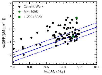
Figure 5: SFR vs. stellar mass for the 81 dwarf galaxies in our sample. We calculated the SFR using GALEX and WISE data as described in Section 2.2. The star forming main sequence from McGaugh et al. (2017) is shown as a blue solid line, and the 1-$\sigma$ intrinsic scatter in the fit is shown by the two blue dashed lines. A total of 37 objects lie above the 1-$\sigma$ scatter of the relation, indicating the presence of vigorous star formation.

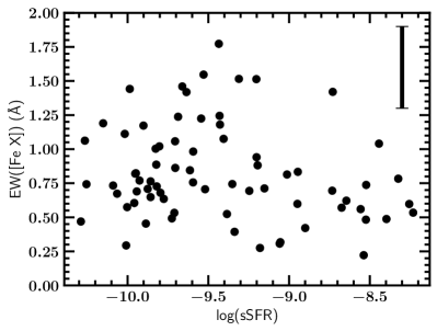
Figure 6: The [Fe X]$\lambda$6374 EW vs. mass-specific SFR for the [Fe X]$\lambda$6374-emitting dwarf galaxy sample. We show the characteristic uncertainty for [Fe X] EW in the top right. We note that there is no clear trend, indicating that the [Fe X] emission is likely not related to stellar processes associated with young stellar populations. Similarly, we see no trend with the [Fe X] luminosity and the mass-specific SFR. See Section 7.1 for a more in-depth discussion.

3 Additional Spectral Analysis

In addition to searching for [Fe X]$\lambda$6374 in the SDSS spectra of dwarf galaxies as described above, we are also interested in searching for AGN activity using other diagnostic emission lines. We created custom codes in python to subtract the stellar continuum, separate the broad and narrow components in H$\alpha$ and H$\beta$ and measure the fluxes of various emission lines. Our codes used the same packages described in Section 2 as well as the Penalized PiXel-Fitting (pPXF; Cappellari, 2017) code to fit the stellar continuum. While pPXF can fit both the emission lines and the stellar continua simultaneously, we wrote our own emission-line fitting software that follows the methodology described in Reines et al. (2013).

3.1 Stellar Continuum Subtraction

Most of the galaxies in our sample are quite blue, indicating a significant amount of star formation. The stellar continuum, which usually dominates the continuum in the SDSS spectra, can contain stellar absorption lines which can severely affect our hydrogen Balmer emission-line measurements. This is especially true for potential weak broad H$\alpha$ and H$\beta$ emission. We therefore remove the stellar continuum using the pPXF fitting code. As our primary goal is to measure the emission lines, we sought good fits to the stellar continua but did not fully explore the entire parameter space.

We used the Bruzual & Charlot (2003, BC03) template spectra, which were used in Tremonti et al. (2004). They were originally selected to describe the SDSS-DR1 galaxies in the $D_{n}(4000)$–H$\delta_{A}$ plane. The template spectra include instantaneous burst single stellar population (SSP) models at ten different ages (0.005, 0.025, 0.10, 0.29, 0.64, 0.90, 1.4, 2.5, 5, and 11 Gyr) and three different metallicities ($Z=0.008,0.02,0.05$). For the 81 galaxies in our sample, we modeled the spectra with pPXF using single-metallicity SSP models and a low-order multiplicative polynomial to account for reddening due to extinction. We accepted the fit for the template family with the lowest reduced $\chi^{2}$, which for all cases was the sub-solar $Z=0.008$ models. One object, NSA 50, did not show any stellar absorption lines and pPXF did not fit any stellar templates to the galaxy continuum. For this object, we employed a third-order polynomial to remove the continuum emission in the SDSS spectrum. We show an example of a stellar continuum fit in the top panel of Figure 7.

3.2 Emission Line Measurements

We fitted the emission lines in the continuum-subtracted SDSS spectra following the same methodology as Reines et al. (2013). We include a linear fit to the continuum in all of the emission-line fitting processes described below to account for uncertainty associated with the stellar continuum fit.

We first fit the [S II]$\lambda\lambda$6716,6731 doublet with a single Gaussian for each line, assuming the same width in velocity, and constraining their separation according to their laboratory wavelengths. We then perform a second fit on [S II]$\lambda\lambda$6716,6731, but using two Gaussians per line. In this case, we constrain the relative heights, widths and positions of the two-component model to be the same for the two lines. We accept the 2-Gaussian model if the reduced $\chi^{2}$ is at least 10% lower than that of the single Gaussian model.

We then use the [S II] model as a template for the [N II]$\lambda\lambda$6548,6583 doublet and the narrow component of the H$\alpha$ line as all three are known to have well-matched profiles (e.g., Filippenko & Sargent, 1988, 1989; Ho et al., 1997; Greene & Ho, 2004; Reines et al., 2013). Specifically, we require that the widths are the same in velocity for the single-Gaussian model, and the relative velocity widths, position and height ratios are constrained to be the same in the 2-Gaussian model. If the [S II] model is a single Gaussian, we allow the H$\alpha$ narrow line width to increase by as much as 25%. This constraint accounts for the fact that H$\alpha$ is emitted physically closer to the power source than [S II] (Ho, 2008) and thus likely has a broader profile, and has been shown to accurately describe the narrow H$\alpha$ emission seen in dwarf galaxies by Reines et al. (2013). For the [N II] doublet, we further constrain the relative flux to be [N II]$\lambda$6583/[N II]$\lambda 6548=3$. This fit is performed again, this time with the inclusion of a broad H$\alpha$ component. We accept the broad+narrow H$\alpha$ fit if the reduced $\chi^{2}$ is at least 20% smaller than that of the narrow-only H$\alpha$ fit, and the broad H$\alpha$ component has a FWHM of at least 500 km s^-1. We accept the [O I]$\lambda\lambda$6300,6363 and [Fe X]$\lambda$6374 measurement as described in Section 2.1 as there are no strong stellar absorption lines in that spectral region. We then fit the H$\beta$ emission line both with and without a broad component, using the same constraints used for the H$\alpha$ line. We accept the broad+narrow component fit if the reduced $\chi^{2}$ is 20% lower than the narrow-only fit.

Finally, we perform fits on the [O III]$\lambda\lambda$4959,5007 doublets, as well as the He II$\lambda$4686, [Fe VII]$\lambda$6087, and [O II]$\lambda\lambda 7320,7330$ emission lines. We fit the [O III] emission with one- and two-Gaussian models, and accept the two-Gaussian model if the reduced $\chi^{2}$ is improved by at least 20%. We placed no constraints on the [Fe VII]$\lambda$6087 and He II$\lambda$4686 emission lines apart from only using a single-Gaussian fit. We constrained the widths of the [O II]$\lambda\lambda 7320,7330$ doublet to be the same, but did not put any constraints on the flux ratio. The broad- and narrow-line measurements for all lines except [Fe X]$\lambda$6374 are given in Table 3, and the [Fe X]$\lambda$6374 measurements are given in Table 2. We show example fits for all the measured emission lines in Figure 7.

Table 3: Emission Line Fluxes

NSAID	He II$\lambda 4686$	H$\beta$(n)	H$\beta$(b)	[O III]$\lambda 5007$	[O I]$\lambda 6300$	H$\alpha$(n)	H$\alpha$(b)	[N II]$\lambda 6583$	[S II]$\lambda 6716$	[S II]$\lambda 6731$	[O II]$\lambda 7320$	[O II]$\lambda 7330$
50	$77\pm 6$	$6740\pm 40$	$\dots$	$38100\pm 300$	$188\pm 6$	$29400\pm 200$	$\dots$	$282\pm 4$	$630\pm 6$	$499\pm 5$	$149\pm 5$	$121\pm 5$
6055	$\dots$	$82\pm 5$	$\dots$	$80\pm 20$	$14\pm 3$	$289\pm 4$	$\dots$	$61\pm 2$	$75\pm 3$	$55\pm 3$	$\dots$	$\dots$
10870	$\dots$	$37\pm 5$	$\dots$	$35\pm 5$	$6\pm 2$	$116\pm 4$	$\dots$	$28\pm 2$	$37\pm 4$	$20\pm 3$	$\dots$	$\dots$
15288	$\dots$	$464\pm 6$	$\dots$	$2110\pm 50$	$37\pm 3$	$1560\pm 20$	$\dots$	$80\pm 2$	$123\pm 4$	$97\pm 3$	$12\pm 5$	$13\pm 4$
21569	$\dots$	$294\pm 8$	$\dots$	$680\pm 10$	$32\pm 4$	$1152\pm 9$	$\dots$	$120\pm 3$	$174\pm 5$	$124\pm 4$	$11\pm 3$	$9\pm 3$
30143	$\dots$	$95\pm 3$	$\dots$	$244\pm 7$	$10\pm 2$	$295\pm 7$	$\dots$	$25\pm 2$	$49\pm 4$	$34\pm 3$	$\dots$	$\dots$
41675	$26\pm 7$	$3140\pm 20$	$\dots$	$15900\pm 100$	$89\pm 5$	$9300\pm 100$	$150\pm 30$	$305\pm 4$	$521\pm 8$	$383\pm 7$	$66\pm 4$	$50\pm 3$
46653	$\dots$	$57\pm 3$	$\dots$	$72\pm 3$	$7\pm 1$	$196\pm 4$	$\dots$	$41\pm 1$	$49\pm 2$	$37\pm 2$	$\dots$	$\dots$
50800	$\dots$	$1960\pm 20$	$\dots$	$11400\pm 300$	$100\pm 5$	$6760\pm 60$	$100\pm 10$	$239\pm 3$	$394\pm 7$	$276\pm 5$	$56\pm 3$	$45\pm 3$
61382	$\dots$	$55\pm 3$	$\dots$	$130\pm 40$	$10\pm 3$	$172\pm 4$	$\dots$	$16\pm 1$	$33\pm 2$	$20\pm 2$	$\dots$	$\dots$

Note. — The entirety of Table 3 is published in the electronic edition of The Astrophysical Journal. We show a portion here to give information on its form and content. All fluxes are presented in units of $10^{-17}$ erg s^-1 cm^-2, and are not corrected for reddening. While the weaker lines in the [O III] and [N II] doublets were simultaneously fit with the stronger doublet line, we do not list their fluxes as they are weaker by a fixed factor of 3. The [O I] doublet is fit as described in Section 2.1. H$\alpha$ and H$\beta$ fluxes are split into the narrow (n) and broad (b) components, where applicable.

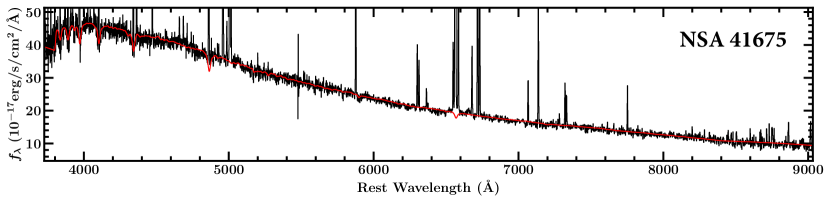
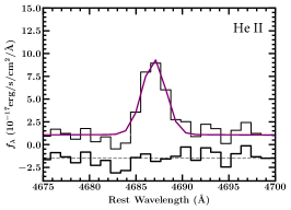
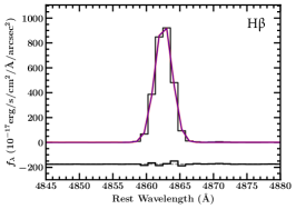
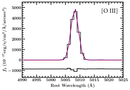
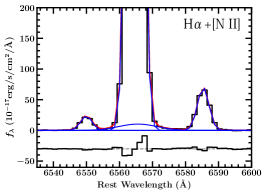
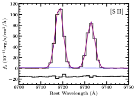
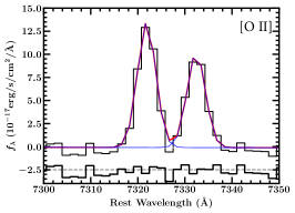
Figure 7: Top: The redshift-corrected spectrum of NSA 41675. The data are in black and the stellar continuum fit is over-plotted in red. Middle and Bottom: The emission-line fits for NSA 41675 on the continuum-subtracted spectrum. We do not show the [O I]$\lambda\lambda$6300,6363 and [Fe X]$\lambda$6374 fits as they are presented in Figure 1. The data are shown in black, the total model is over-plotted in red and the individual components are shown in blue. The residuals are shown below each fit. See Section 3.3.2 for details.

3.3 AGN Indicators

The 81 [Fe X]-emitting dwarf galaxies presented in this work are considered strong AGN candidates given their high [Fe X] luminosities ($L_{\rm[FeX]}\gtrsim 10^{36}$ erg s^-1). In order to search for additional evidence of AGN activity, we employed several supplemental AGN detection techniques using our emission-line measurements. We note that the vigorous star formation seen in the host galaxies may dilute or effectively hide the AGN signal in more traditional emission-line diagnostic indicators, similar to the two previously detected AGN with coronal-line emission, J1220+3020 and Mrk 709S (see Molina et al., 2021; Kimbro et al., 2021, for details). We describe each detection technique in detail below.

3.3.1 He II and [Fe VII]$\lambda$6087

The emission line He II $\lambda 4686$ has a relatively high ionization potential (54.4 eV), and thus needs a hard ionization field to be produced. Therefore, luminous He II detections can be a useful indicator of AGN activity. The log(He II/H$\beta)$ ratio has been used to search for AGN activity in dwarf galaxies by Sartori et al. (2015), given that He II is less affected by star formation than [O III]$\lambda 5007$. In our sample, 5 objects show He II emission with a $\rm{S/N}>3$. We adopt a stricter criterion than Sartori et al. (2015) for AGN selection, setting a limit of log(He II/H$\beta)>-1$ as neither X-ray Binaries (XRBs) nor Wolf-Rayet (WR) stars can reproduce that line ratio (Shirazi & Brinchmann, 2012; Schaerer et al., 2019). We find that 4 out of the 5 objects (NSA IDs 50, 41675, 256802 and 275961) meet this criterion. We therefore consider these objects as very strong AGN candidates given their [Fe X] and He II emission. Meanwhile, the only object to exhibit [Fe VII]$\lambda$6087 emission is NSAID 256802, which was previously identified as an AGN in Reines et al. (2013, their ID 20).

3.3.2 Broad H$\alpha$

Virialized gas that orbits close to a BH will exhibit broad-line emission due to the bulk motion of the gas. This emission will be most clearly seen in the recombination hydrogen Balmer lines, particularly H$\alpha$ as it is less affected by dust attenuation than H$\beta$. However, not all AGNs exhibit broad-line emission (see Ho, 2008, and references therein), and we therefore do not exclude objects without broad-line emission from our AGN candidate sample. We detected strong broad H$\alpha$ emission ($L[{\rm H}\alpha]>10^{40}$ erg s^-1) in 2/81 objects. Both galaxies, NSA 256802 and 427201, were included in Reines et al. (2013, their ID 20 and ID N). NSA 256802 was determined to be a broad-line AGN by Reines et al. (2013). While NSA 427201 was classified as star-forming with broad H$\alpha$ emission in Reines et al. (2013), we note that it could be a TDE (See Section 7.1). Weak broad-line emission ($L[{\rm H}\alpha]<10^{40}$ erg s^-1) was detected in an additional 9 BPT star-forming objects, but since weak broad H$\alpha$ can be produced by stellar processes (e.g., Baldassare et al., 2016), the origin of the broad H$\alpha$ is unclear.

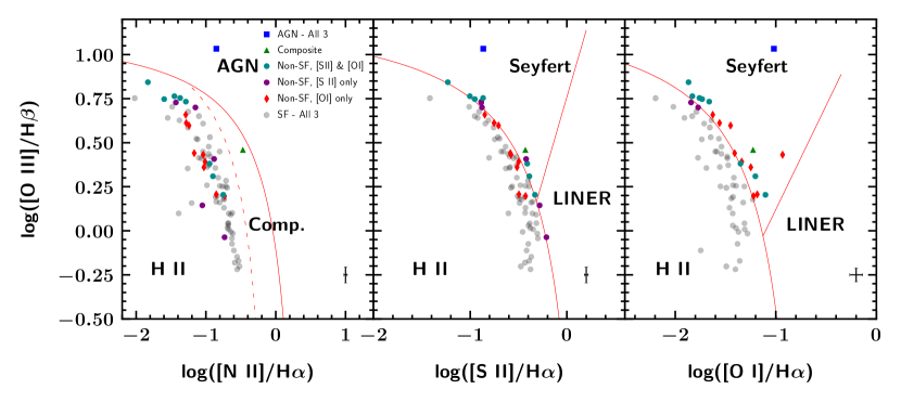
Figure 8: The BPT or VO87 diagrams for the 81 objects in our sample. Given their high [Fe X] luminosities, all of these objects are considered strong AGN candidates whose AGN signal may be hidden in traditional diagnostics due to the intense host-galaxy star formation. The theoretical extreme starburst and Seyfert lines from Kewley et al. (2006) are shown as solid red lines, while the empirical composite line from Kauffmann et al. (2003) is shown as the red dashed line. We show characteristic uncertainties for each line ratio in the bottom right corner of each panel. One object is AGN-like in all three diagrams (shown by the blue square), and one object falls in the composite region (green triangle). Both of these objects are also in the Reines et al. (2013) survey (IDs 20 and 105, respectively). Of the remaining objects, 10% are non-star-forming in both the [S II]/H$\alpha$ and [O I]/H$\alpha$ diagrams (shown as teal circles), 6% are non-star-forming in only the [S II]/H$\alpha$ diagram (shown as purple circles), and 11% are non-star-forming in only the [O I]/H$\alpha$ diagram (red diamonds).

3.3.3 Narrow Line Diagnostic Diagrams

Diagnostic emission-line ratio diagrams can help separate galaxies dominated by AGN activity from star-forming galaxies. We created the narrow-line diagnostic diagrams shown in Figure 8, which are presented in Veilleux & Osterbrock (1987, VO87) and are based on the BPT diagrams (Baldwin et al., 1981). These diagrams take [O III]/H$\beta$ versus [N II]/H$\alpha$, [S II]/H$\alpha$, and [O I]/H$\alpha$. We include both the empirical composite line from Kauffmann et al. (2003), and the theoretical extreme starburst lines and Seyfert-LINER lines from Kewley et al. (2006). The AGN and Composite objects denoted by the blue square and green triangle, respectively, are from Reines et al. (2013, their IDs 20 and 105).

Approximately 30% of our sample appears Seyfert- or LINER-like in at least one of the diagnostic diagrams, where 1 object is Seyfert-like in all three diagrams, 10% appear non-star-forming in both the [S II]/H$\alpha$ and [O I]/H$\alpha$ diagrams, 6% are non-star-forming in only the [S II]/H$\alpha$ diagram, and 11% are non-star-forming in only the [O I]/H$\alpha$ diagram. Given the known metallicity dependence of [N II]/H$\alpha$ ratio, the sensitivity of [S II]/H$\alpha$ to shocks, and the inability of standard stellar processes to produce enhanced [O I] emission (e.g., Kewley et al., 2006, 2019; Molina et al., 2018), we consider the objects that show Seyfert or LINER-like [O I] emission to be the strongest AGN candidates based on the VO87 diagrams. We do note that the emission-line ratios from the 3″ SDSS single-fiber spectra for both Mrk 709S and J1220+3020 appear star-forming in all three VO87 diagrams, even though both have confirmed AGN activity and detected [Fe X] emission (Reines et al., 2020; Molina et al., 2021; Kimbro et al., 2021). Therefore, we still consider all of these objects as AGN candidates based on their [Fe X] emission.

In addition to the typical VO87 diagrams, there are near-infrared (NIR) diagnostic diagrams that can be used to distinguish AGN from stellar activity. The [S II]$\lambda\lambda 9069,9531$/H$\alpha$ vs. [S II]$\lambda\lambda 6716,6731$/H$\alpha$, [S II]$\lambda\lambda 9069,9531$/H$\alpha$ vs. [O II]$\lambda\lambda 7320,7330$/H$\alpha$ and [S II]$\lambda\lambda 6716,6731$/H$\alpha$ vs. [O II]$\lambda\lambda 7320,7330$/H$\alpha$ from Osterbrock et al. (1992) were recently used by Bohn et al. (2021) to determine the presence of AGN activity in dwarf galaxies. Given the wavelength range of the SDSS spectra, we utilize only one of the three diagrams, [S II]$\lambda\lambda 6716,6731$/H$\alpha$ vs. [O II]$\lambda\lambda 7320,7330$/H$\alpha$ to search for AGN activity in our sample. We show this diagram in Figure 9.

These diagrams are strictly empirical, and so we employ cuts in our data to identify objects that are clustered with the Seyfert-like objects in the diagram, denoted by the dark-blue dashed line in Figure 9. We employ a purity cut, such that all H II regions are avoided in our AGN selection region. We thus consider the 16 objects with log([S II]$\lambda\lambda 6716,6731$/H$\alpha)>-0.7$ and log([O II]$\lambda\lambda 7320,7330$/H$\alpha)>-1.95$ to be strong AGN candidates based on this NIR diagnostic diagram and their strong [Fe X] emission. We present the results of both the VO87 and NIR diagnostic diagrams in Table 4.

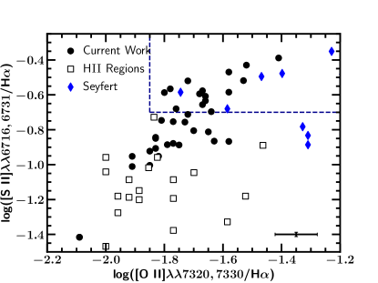
Figure 9: The log([S II]$\lambda\lambda 6716,6731$/H$\alpha$) vs. log([O II]$\lambda\lambda 7320,7330$/H$\alpha$) diagram for our sample. Here we only include the 36 objects that have [O II]$\lambda\lambda 7320,7330$ detections. The data from this work are shown as black filled circles, and the star forming or H II regions and Seyfert galaxies from Osterbrock et al. (1992) are shown as unfilled squares and blue diamonds, respectively. The characteristic error bars for the line ratios in our sample is shown in the bottom left. The dashed box indicates the region we consider AGN-like given the clustering of the Seyfert and H II region data. 16 out of the 36 objects with [O II]$\lambda\lambda 7320,7330$ detections are consistent with AGN activity. We note that given their high [Fe X] luminosities, all of these objects are considered strong AGN candidates whose AGN signal may be hidden in traditional diagnostics due to the intense host-galaxy star formation.

Table 4: Results of Narrow-Line Diagnostic Diagrams

	VO87 Diagrams			NIR Diagram
NSA ID	[N II]/H$\alpha$	[S II]/H$\alpha$	[O I]/H$\alpha$	[O II]/H$\alpha$
(1)	(2)	(3)	(4)	(5)
50	SF	Sy	Sy	SF
15288	SF	SF	Sy	SF
21569	SF	SF	SF	AGN
50800	SF	Sy	Sy	SF
61382	SF	SF	Sy	…
63560	SF	SF	SF	AGN
95985	SF	Sy	Sy	SF
102990	SF	SF	SF	AGN
140290	SF	Sy	Sy	…
140756	SF	Sy	SF	…
141686	SF	Sy	Sy	…
144266	SF	SF	Sy	AGN
162936	SF	LINER	SF	…
164449	SF	Sy	SF	…
174326	SF	SF	SF	AGN
213780	SF	SF	SF	AGN
220716	SF	SF	Sy	…
237974	SF	SF	Sy	…
256802	AGN	Sy	Sy	SF
270622	SF	Sy	Sy	…
275961	Comp.	Sy	Sy	AGN
300542	SF	Sy	Sy	AGN
305229	SF	Sy	Sy	SF
328894	SF	Sy	Sy	…
345375	SF	SF	Sy	AGN
393631	SF	SF	SF	AGN
401495	SF	Sy	SF	…
426824	SF	SF	Sy	…
442120	SF	SF	SF	AGN
442212	SF	Sy	Sy	SF
442427	SF	LINER	SF	…
457940	SF	Sy	Sy	…
458829	SF	Sy	Sy	SF
491412	SF	SF	Sy	SF
501341	SF	Sy	SF	SF
524413	SF	SF	Sy	…
532026	SF	SF	SF	AGN
553772	SF	SF	SF	AGN
577169	SF	SF	SF	AGN
656364	SF	SF	SF	AGN
670127	SF	SF	SF	AGN

Note. — We only present objects that are Seyfert (Sy), Composite (Comp.), LINER or AGN-like in at least one diagram in this table. The remaining 40 objects were either star-forming in all three VO87 diagrams, and are either consistent with star formation or do not have detected [O II] emission needed for the NIR diagram. Column (1): NSA IDs. Columns (2-4): Classifications from the [O III]/H$\beta$ vs. [N II]/H$\alpha$, [S II]/H$\alpha$, and [O I]/H$\alpha$ diagrams, as shown in Figure 8. Column (5): NIR [S II]/H$\alpha$ vs. [O II]/H$\alpha$ diagram as shown in Figure 9.

4 Optical Variability

The variability observed in some AGN light curves is well-described by a damped random walk (DRW) model (e.g., Kelly et al., 2009; MacLeod et al., 2010), which is distinct from the variability expected from supernovae and supernova remnants (i.e., a clear decline in brightness after the initial peak post-explosion). While studying optical variability is a well-known technique used to detect AGN activity in high-mass galaxies, recent work by Baldassare et al. (2018, 2020) has demonstrated that it can be effective in identifying optically-variable AGN in the dwarf galaxy regime.

In order to search for AGN-like variability in our sample, we created and analyzed light curves of the physical region covered by the SDSS spectroscopic fiber using data from the Palomar Transient Factory (PTF; Rau et al., 2009; Law et al., 2009). The PTF is a wide-field optical survey designed to systematically explore the optical variable and transient sky. Data collection for the PTF began in 2009, which is $\sim 9$ years after a majority of the SDSS single-fiber spectra were taken. Conversely, most of the optical decline seen in supernovae occur within the first 3–5 years (e.g. Filippenko, 1997; Smith et al., 2009, 2017). Therefore, while we can search for variability consistent with a DRW model and thus indicative of AGN activity, we may not be able to attribute signatures of SNe-like variability to the observed emission seen in the SDSS spectra.

4.1 Data Analysis and Results

We followed the methodology first presented in Baldassare et al. (2020), which we briefly describe here. We rely on the $R$-band images from PTF as they have significantly better sky coverage, long baselines and larger number of observations than the $g$-band data, and limit our data collection to PTF images with seeing better than 3″. These cuts result in approximately 70 observations per object. We then create a template of the host galaxy emission using the Difference Imaging and Analysis Pipeline 2 (DIAPL2), which is a modified version of the Difference Imaging Analysis software (Wozniak, 2000). This template is then modified to match the seeing and background levels of each individual exposure. The template is then subtracted from each exposure creating a difference image.

We then construct light curves by performing aperture photometry on the template and difference images, such that the flux value for each data point is the template plus the difference image measurements. We use an aperture of 3″ centered on the position of the SDSS fiber as listed in the NSAv1. After our light curves are constructed, we search for DRW-like variability using the software QSO_fit (Butler & Bloom, 2011). Objects are then classified as candidate variable AGN if they have $\sigma_{\rm var}>2$, $\sigma_{\rm QSO}>2$ and $\sigma_{\rm QSO}\gtrsim\sigma_{\rm notQSO}$. Here, $\sigma_{\rm var}$ gives the significance that the object is variable; $\sigma_{\rm QSO}$ is the significance that the $\chi^{2}$ for the DRW model is better than that for non-AGN-like variability and $\sigma_{\rm notQSO}$ gives the significance that the source variability is better described by random variability. Out of the 50 total objects with adequate PTF data, the only galaxy to show AGN-like variability was NSA 131809 (NSAv0 26828), which was also detected as variable AGN candidate in Baldassare et al. (2020). We also found supernova-like variability in NSA 331627, however this SNe event occurred about 7 years after the SDSS spectrum was taken and thus it cannot explain the observed [Fe X] emission. We note that the previously identified AGN NSA 256802 (ID 20 from Reines et al., 2013) did not exhibit variability in the PTF data, demonstrating that not all AGN may be optically variable. We therefore do not exclude any objects as AGN candidates based on this detection technique.

5 X-ray Detections

Table 5: Chandra Observations

NSAID	Date observed	Obs ID	Exp. time (ks)	$N_{\rm background}$
256802	2010 Jul 25	11464	1.8	0.0034
533731	2013 Jan 13	13929	20.8	0.0075
472272	2013 Jun 02	14911	15.8	0.0062
625882	2018 Jun 06	19441	29.6	0.1417
50	2017 Mar 11	19463	14.9	0.1199
275961	2018 Aug 17	20773	15.0	0.1751

Note. — $N_{\rm background}$ is the number of expected 2-10 keV $N(>S)$ background sources within $3r_{50}$, using Moretti et al. (2003).

Table 6: X-ray Sources

NSAID	R.A.	Decl.	Offset	Net Counts		Flux ($10^{-15}$ erg s-1 cm-2)		Luminosity (log(erg s-1))
	(deg)	(deg)	(arcsec)	0.5-2 keV	2-7 keV	0.5-2 keV	2-10 keV	0.5-2 keV	2-10 keV
(1)	(2)	(3)	(4)	(5)	(6)	(7)	(8)	(9)	(10)
256802$-$X1	185.928452	58.246088	0.3	296.50$\pm 29.78$	124.76$\pm 19.94$	719.25	1475.86	41.6	41.8
533731$-$X1	147.325040	16.878966	0.3	23.31$\pm 8.92$	8.55$\pm 5.26$	5.73	8.88	40.5	40.7
472272$-$X1	245.468974	15.315684	0.5	9.27$\pm 5.32$	3.08${}^{+4.11}_{-2.46}$	3.20	4.31	39.9	40.0
625882$-$X1	166.283858	44.748226	6.4	10.26${}^{+7.47}_{-4.91}$	7.25$\pm 4.92$	2.91	5.52	39.4	39.7
625882$-$X2	166.284416	44.747104	2.8	17.40$\pm 7.79$	15.01${}^{+8.72}_{-6.12}$	4.94	11.41	39.7	40.0
625882$-$X3	166.284419	44.747115	2.8	9.00$\pm 5.29$	$\cdots$	2.56	$<$1.67	39.4	$<$39.2
50$-$X1	146.008247	$-0.643140$	3.5	95.64$\pm 17.31$	67.44$\pm 14.89$	49.44	100.45	39.5	39.8
50$-$X2	146.007968	$-0.642340$	0.7	5.17${}^{+4.87}_{-3.22}$	12.22${}^{+8.15}_{-5.47}$	2.68	18.23	38.2	39.0
275961$-$X1	207.855629	40.213289	0.3	10.54${}^{+7.41}_{-4.87}$	36.25$\pm 11.1$	6.09	55.24	38.9	39.9

Note. — Column 1: Identification number in the NSA. Column 2: right ascension of hard X-ray source (when present). Column 3: declination of hard X-ray source (when present). Column 4: distance between hard X-ray source and center of SDSS spectroscopic Fiber. Columns 5-6: net counts after applying a 90% aperture correction. Error bars represent 90% confidence intervals. Columns 7-8: fluxes corrected for Galactic absorption. Columns 9-10: log luminosities corrected for Galactic absorption; calculated using a photon index of $\Gamma=1.8$.

Hard X-ray photons are emitted by the hot corona surrounding the accretion disk (e.g., Liang & Nolan, 1984; Haardt & Maraschi, 1991). If the observed hard X-ray luminosity is much larger than that expected from X-ray binaries, this can signify the presence of an AGN in a galaxy. However, AGNs with low luminosities (e.g., due to low accretion rates) may not exhibit enhanced X-ray emission. To search for AGN activity at X-ray wavelengths, we cross-referenced our sample with the Chandra data archive using a search radius of 5″. Out of the 81 galaxies in our sample, 6 have been previously observed. The Chandra observations were taken between 2010 Jul 25 and 2018 Aug 17, with exposure times ranging between 1.8 and 29.6 ks, as summarized in Table 5. While some of these objects have been presented in various references (e.g., Dong et al., 2012; Reines et al., 2014; He et al., 2019; Kimbro et al., 2021), we downloaded the data and performed a consistent analysis for this work. We followed the general methodology laid out in Latimer et al. (2021), which we summarize below.

5.1 Data Reduction and Measurements

We used CIAO v4.13 (Fruscione et al., 2006) to reduce each observation, applying calibration files (CALDB 4.9.5) to create new level 2 event files. We then aligned the Chandra astrometry to the SDSS frame. We created a list of X-ray point sources on the S3 chip using wavdetect on the image filtered from 0.5-7 keV, excluding any wavdetect sources falling within 3$r_{50}$ of the target galaxy. We then used the CIAO function wcs_match to match the remaining X-ray sources to optical point sources in the SDSS DR12 catalog with $i$-band magnitudes $<22$. This resulted in updated astrometry for four of the six galaxies, with astrometric shifts ranging between $\pm$0.12-1.70 pixels ($0\farcs 06$-$0\farcs 83$).

Next we searched for X-ray point sources that could indicate the presence of AGNs in the galaxies. First, we checked our images for background flares and remove time intervals where the background rate was $>3\sigma$. We then re-ran wavedetect on the corrected images of the S3 chip, filtered from 0.5-7 keV. We also set a significance threshold of $10^{-6}$, corresponding to approximately one false source detection over the entire S3 chip. Further analysis is restricted to wavdetect sources that lie within 3$r_{50}$ of the target galaxies.

We extracted source counts using circular apertures corresponding to the 90% enclosed energy fraction at 4.5 keV, or ${\sim}2\arcsec$ for our X-ray sources. Background counts were estimated using source-centered circular annuli having an inner radius equal to the source aperture radius and an outer radius of $12~{}\times$ the inner radius. We considered a source to be detected if the source counts are above the background counts in the source aperture to within a 95% confidence level, following the Bayesian methods in Kraft et al. (1991) for Poisson counting statistics in the presence of a background. All detected sources pass this test.

We calculated net counts by subtracting the background counts in the source aperture from the source counts and applying a 90% aperture correction. We detected a total of nine X-ray point sources across six galaxies, and report their properties in Table 6. An additional X-ray source was detected near NSAID 275961; we exclude this from analysis because it was $\sim 24\arcsec$ offset from the SDSS spectroscopic fiber, which is 3 times larger than the $r$-band half-light radius and thus not within the galaxy. Unabsorbed hard (2-10 keV) and soft (0.5-2 keV) X-ray fluxes are calculated using the CIAO function srcflux. We use Galactic column densities from Dickey & Lockman (1990) maps and a power-law spectral model with photon index $\Gamma=1.8$, which is typical for low-luminosity AGN (Ho, 2008, 2009) and ultraluminous X-ray sources at these energies (Swartz et al., 2008). The 2-10 keV luminosities have a range of log$(L_{\rm 2-10keV}/{\rm erg~{}s}^{-1})=39.0$–$41.8$. We use the estimated minimum fluxes to provide upper limits on X-ray source luminosities for sources that are not detected in both bands (e.g. source X3 in NSAID 625882). Table 6 summarizes the unabsorbed fluxes and corresponding luminosities. Any potential absorption intrinsic to the sources is not accounted for, so these values should be taken as lower limits.

We estimated hardness ratios using the Bayesian Estimation of Hardness Ratios code (BEHR; Park et al., 2006), as it is useful in the Poisson regime of low counts and additionally works even if only one of the hard or soft bands has a source detection. Here we define hardness ratio as $(H-S)/(H+S)$, where $H$ and $S$ are the number of detected counts in the hard (2-7 keV) and soft (0.5-2 keV) X-ray bands, respectively. We have nine X-ray sources with detections in at least one of the two bands, with the resulting hardness ratios displayed in Figure 10. We also use the Portable, Interactive Multi-Mission Simulator (PIMMS) to estimate the hardness ratios for unabsorbed power laws with $\Gamma=1.8$, 2.0, and 2.5. We plot these in Figure 10 as well.

We estimated the 95% positional uncertainties for each source using Equation 5 from Hong et al. (2005), an empirical formula involving the wavdetect counts and off-axis position of the sources. Error bars on net counts represent 90% confidence intervals. For source counts $<10$, we calculate errors using the formalism of Kraft et al. (1991), which takes background counts into account. For source counts $\geq 10$ we use confidence intervals from Gehrels (1986), which assume negligible background counts.

Finally, we find how many background X-ray sources we would expect to fall within 3$r_{50}$ of the target galaxy. We use Equation 2 from Moretti et al. (2003), which takes in an input flux and returns the expected number of background sources we would expect to see with that flux or higher (per square degree). For our input fluxes we use our minimum flux sensitivity, which we estimate by assuming a source with 2 counts. The resulting 2-10 keV (0.5-2 keV) minimum fluxes range from $S_{min}\sim 1.7\textrm{-}26.2$ ($0.5\textrm{-}5.1$) in units of $10^{-15}$ erg s^-1 cm^-2 for the six Chandra observations. Using these fluxes results in the expected number of hard band (soft band) background sources within 3$r_{50}$ of our target galaxies ranging between ${\sim}$0.003-0.175 (0.006-0.121).

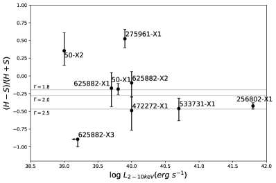
Figure 10: Hardness ratio vs. log 2-10 keV X-ray luminosity for our 9 X-ray sources that were detected in at least one of the two bands. The hardness ratio was calculated using BEHR (see Section 5.1). The error bars are the 68% confidence intervals. Hardness ratios for unabsorbed power laws with $\Gamma=1.8$, 2.0, and 2.5 are shown as grey solid lines.

5.2 Contribution from X-ray Binaries

We compared the measured X-ray emission to that expected from XRBs in order to search for enhanced X-ray emission that would likely indicate the presence of an AGN. The expected galaxy-wide X-ray luminosity from XRBs scales with SFR for high-mass XRBs (Grimm et al., 2003) and with stellar mass for low-mass XRBs (Gilfanov, 2004). Using the relation from Gilfanov (2004) to estimate the expected low-mass XRB luminosities from stellar masses, we find that our observed X-ray luminosities are higher than the expected low-mass XRB luminosities by at least ${\sim}1.3$ dex. We conclude that low-mass XRBs are unlikely to meaningfully contribute to the X-ray luminosities of our observed sources, and thus limit our focus to high-mass XRBs (HMXRBs).

We generally follow the same method as outlined in Latimer et al. (2021). To predict the expected X-ray luminosity from HMXRBs, we use the model from Lehmer et al. (2021), which relates the gas-phase metallicity, SFR, and expected XRB X-ray luminosity. Note that the X-ray luminosities used in this model are in the 0.5-8 keV band; to match, we re-analyze our Chandra data in this band, following the same methodology presented in Section 5.1. Also, while the scatter in the Lehmer et al. (2021) relation is metallicity-dependant, for metallicities $>8.0$ the scatter is more consistent and we find a 1$\sigma$ scatter of ${\sim}0.2$ dex. This applies to all of our X-ray detected galaxies with the exception of NSAID 50. We use the SFRs and metallicities described in Section 2.2, which are summarized in Table 1.

A comparison between the expected cumulative XRB luminosity for each galaxy and our observed galaxy-wide X-ray luminosities can be seen in Figure 11. Two galaxies have observed values significantly ($>3\sigma$) above expectations for XRBs: NSAIDS 256802 and 275961, which are ${\sim}15\sigma$ and ${\sim}3.5\sigma$ higher than the expected values from XRBs, respectively. We therefore consider these two objects X-ray-detected AGNs. In addition to the archival Chandra data analyzed here, we note that one other galaxy in our sample, NSA 95985 (SDSS J153704.18+551550.5), was determined to be an X-ray-selected AGN candidate by Birchall et al. (2020), who utilized the 3XMM DR7 catalog (Rosen et al., 2016) to search for AGN activity.

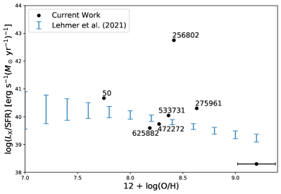
Figure 11: Log ratio of X-ray luminosity over host galaxy SFR vs. metallicity. The values and error bars in blue are the expected X-ray luminosity from XRBs from Lehmer et al. (2021). The ${\sim}0.18$ uncertainty in the metallicities is shown in black in the lower right-hand corner. While only two objects (NSA 256802 and 275961) are X-ray-detected AGNs, we still consider all of the objects in our sample as AGN candidates due to their strong [Fe X] emission.

6 Radio Detections

6.1 Catalog Data

Almost all AGNs, including LLAGNs produce radio emission, which is not obscured by dust attenuation (see Ho, 2008, and references therein). Additionally, bright radio emission consistent with an accreting BH was seen in both Mrk 709S (Reines et al., 2014; Kimbro et al., 2021) and SDSS J122011.26+30200 (ID82; Reines et al., 2020; Molina et al., 2021), both of which also presented strong [Fe X]$\lambda$6374 emission in their optical spectra. Therefore, we cross-referenced our sample of [Fe X]-detected dwarf galaxies with both the Very Large Array (VLA) Faint Images of the Radio Sky at Twenty-centimeters (FIRST) survey (Becker et al., 1995) and the first epoch of the Very Large Array Sky Survey (VLASS; Lacy et al., 2020) using a maximum separation of 5″. The single-epoch VLASS data comprises 3 GHz observations with a spatial resolution of 2$\farcs$5, and a sensitivity threshold of $\approx 0.12$ mJy, while the FIRST survey includes 1.4 GHz observations with a sensitivity of 0.15 mJy and a spatial resolution of 5″. Five total objects have FIRST detections, and three of those are also detected in VLASS. The FIRST and VLASS Quick Look Catalog (Gordon et al., 2020) detections and integrated fluxes for our sample are given in Table 7, and the FIRST radio detections are shown in Figure 12. We note that two objects in our sample, NSA 427201 and 50, were also in the Reines et al. (2020) VLA sample as their IDs 98 and 38, respectively.

Table 7: Radio Detections

NSAID	FIRST		VLASS
	$S_{1.4~{}\textrm{GHz}}$	Offset	$S_{3~{}\textrm{GHz}}$	log($L_{3~{}\textrm{GHz}}$)	Major Axis	Minor Axis	P.A.	Offset
472272	1.07	0.9	…	…	…	…	…	…
50	1.30	0.4	…	…	…	…	…	…
427201	1.59	2.1	$0.7\pm 0.2$	$21.30$	$3.0\pm 0.6$	$2.4\pm 0.4$	$166\pm 38$	0.8
533731	3.14	0.8	$1.7\pm 0.5$	21.95	$4\pm 1$	$2.9\pm 0.5$	$53\pm 27$	0.4
625882	11.64	2.5	$5.9\pm 0.7$	21.74	$5.8\pm 0.6$	$4.8\pm 0.4$	$174\pm 24$	0.3

6.2 Contribution from HII Regions, SNRs and SNe

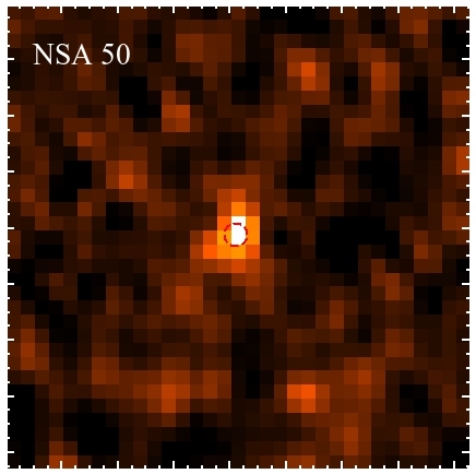
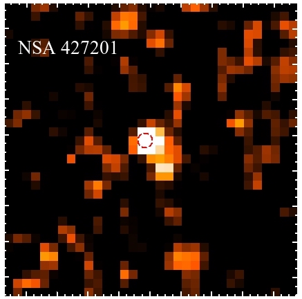
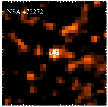
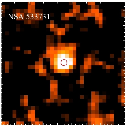
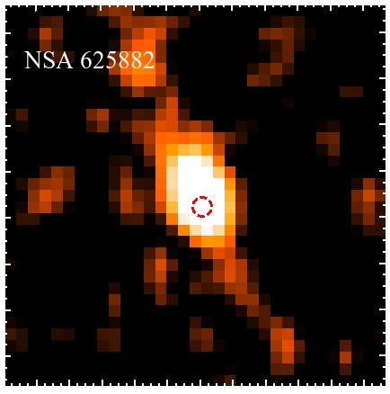
Figure 12: The FIRST 1.4 GHz observations for the 5 detected galaxies in our sample. The red dotted circle shows the position and spatial extent of the SDSS 3″ fiber. Most of the objects have centrally-concentrated radio emission, except for NSA 625882 which clearly extended. All but NSA 50 have radio emission strongly indicating AGN activity. However, all of the objects in our sample are still considered AGN candidates due to their strong [Fe X] emission.

In order to test for radio AGN activity, we employed the same criteria as Reines et al. (2020). We relied on the FIRST 1.4 GHz data in our analysis as all 5 objects are detected in FIRST. We first compared the estimated SFR from the radio source to the global SFR of the galaxy calculated via GALEX+WISE data, assuming that the radio emission is thermal. We used equation 2 from Condon (1992) to calculate the production rate of Lyman continuum photons, $Q_{\textrm{Lyc}}$:

$$\begin{split}\left(\frac{Q_{\textrm{Lyc}}}{s^{-1}}\right)\gtrsim 6.3\times 10^{52}\left(\frac{T_{e}}{10^{4}~{}\textrm{K}}\right)^{-0.45}\left(\frac{\nu}{\textrm{GHz}}\right)^{0.1}\\ \times\left(\frac{L_{\nu,\textrm{thermal}}}{10^{20}~{}\textrm{W~{}Hz}^{-1}}\right).\end{split}$$ (2)

Here, we assume $T_{e}=10^{4}$ K and $\nu=1.4$ GHz to match the FIRST observations. We estimate $Q_{\textrm{Lyc}}\sim 10^{52\mbox{--}54}$ photons s^-1 for all 5 radio sources. We then estimate the instantaneous SFR for the radio source, assuming it is purely thermal, using equation 2 from Kennicutt (1998):

$$\textrm{SFR}(M_{\odot}~{}yr^{-1})=1.08\times 10^{-53}Q_{\textrm{Lyc}}(s^{-1}).$$ (3)

We find that the estimated global SFRs from Section 2.2 are lower than the estimates from the radio detections by a factor of $\sim 2.5\mbox{--}15$, implying that thermal H II regions cannot fully explain the observed radio emission.

We then compared our FIRST detections to that expected from individual supernovae or supernova remnants. In order to estimate the radio luminosity of the brightest supernova or supernova remnant in a galaxy, we use the following equation from Chomiuk & Wilcots (2009):

$$L_{1.4}^{\textrm{max}}=(95^{+31}_{-23})SFR^{0.98\pm 0.12}.$$ (4)

Assuming the estimated global GALEX+WISE SFRs from Section 2.2, we estimate the highest luminosity of an individual SRN/SNe to be $L_{1.4~{}\textrm{GHz}}\approx 0.1\mbox{--}6.6\times 10^{26}$ erg s^-1, which is $\sim 30\mbox{--}260$ times smaller than the measured 1.4 GHz luminosity. We therefore rule out individual SNRs/SNe as the source of the observed radio emission.

Given the large radio emission region, if the origin is stellar it may be due to a population of SNRs/SNe. Following the procedure described in Reines et al. (2020), we calculate the total expected 1.4 GHz luminosity from all SNRs/SNe using the equation

$$L_{\textrm{total}}=\int n(L)\,L\,dL$$ (5)

from Chomiuk & Wilcots (2009) where

$$n(L)=\frac{dN}{dL}=92\times SFR\times L^{-2.07}.$$ (6)

We take the integral from 0.1 to $10^{4}$ in order to probe the entire range of luminosities presented in Chomiuk & Wilcots (2009) and the SFRs from Table 1, resulting in predicted values of $L_{1.4~{}\textrm{GHz}}=0.1\mbox{--}6\times 10^{27}$ erg s^-1. This is lower than the FIRST radio detections in all 5 objects by a factor of $4\mbox{--}27$. We therefore conclude that the 1.4 GHz radio emission cannot be explained solely by population of SNRs/SNe in a majority of our objects.

Table 8: Comparison of Observed Radio Emission to Estimated Values from Stellar Processes

NSAID	SFRrad	SFRrad/SFRFUV+IR	$L^{\rm max}_{\nu}$	$L_{\rm obs}/L^{\rm max}_{\nu}$	$L_{\rm total}$	$L_{\rm obs}/L_{\rm total}$	$L_{\rm HII+SNe}$	$L_{\rm obs}/L_{\rm HII+SNe}$	Class.
(1)	(2)	(3)	(4)	(5)	(6)	(7)	(8)	(9)	10
FIRST Data (1.4 GHz)
472272	17.9	6.1	2.7	93.7	25.0	10.2	6.5	3.9	AGN
50	0.4	2.5	0.2	35.9	1.5	4.1	0.4	1.6	SF
427201	32.2	6.6	4.5	101.3	42.0	10.9	10.9	4.2	AGN
533731	120.6	16.8	6.6	261.3	61.4	27.9	15.9	10.8	AGN
625882	76.7	15.0	4.7	232.0	43.7	25.0	11.3	9.6	AGN
VLASS Data (3 GHz)
427201	14.2	2.9	3.1	65.3	28.7	7.0	10.9	2.2	AGN
533731	65.3	9.1	4.5	207.2	41.9	22.1	15.9	6.8	AGN
625882	38.9	7.6	3.2	172.2	29.8	18.5	11.3	5.7	AGN

Note. — Column (1): NSAID. Column (2): The estimated SFR in units of $M_{\odot}$ yr^-1 using the observed radio emission in either FIRST or VLASS, assuming Equations 2 and 3. Column (3): Comparison of the observed SFR given in Table 1 to estimated SFR from Column 2. Column (4): Estimated maximum 1.4 or 3 GHz luminosity, in units of $10^{26}$ erg s^-1 Hz^-1 for an individual SNe or SNR assuming equation 4. Column (5): Comparison of observed luminosity (FIRST or VLASS) to estimated luminosity from Column 4. Column (6): Total expected luminosity (at either 1.4 or 3 GHz and in units of $10^{26}$ erg s^-1 Hz^-1) for a population of SNe/SNRs, assuming equation 5 and 6. Column (7): Comparison of observed luminosity (FIRST or VLASS) to estimated luminosity from Column 6. Column (8): Summation of expected the luminosity (at either 1.4 or 3 GHz) in units of $10^{20}$ W Hz^-1 from thermal H II regions and populations of SNe, following Equations 2, 3, 5 and 6. Column (9): Comparison of observed luminosity (FIRST or VLASS) to the estimated luminosity from Column 8. Column (10): Classification of observed radio luminosity–“AGN” indicates that the radio emission is too luminous to be consistent with star formation, while “SF” indicates the radio emission is consistent with star formation.

We finally considered a combination of thermal H II emission and population of SNRs/SNe. We summed the measurements from the SNR/SNe population assuming the global GALEX+WISE SFRs as described above with the expected thermal emission from H II regions using the global SFRs given in Table 1. The combination of these two values results in a predicted $L_{1.4~{}{\rm GHz}}=0.04\mbox{--}1.59\times 10^{21}$ W Hz^-1. All objects but NSA 50 have a measured 1.4 GHz luminosity that is a factor of $\gtrsim 4$ higher than the predicted value. We therefore conclude that the 1.4 GHz radio emission in all objects except for NSA 50 is likely the result of AGN activity. We also note that the high-resolution VLA data of NSA 50 studied in Reines et al. (2020, their ID 38) was also consistent with star formation. Therefore, we cannot rule out star formation as the origin of the radio emission in this galaxy.

We performed the same analysis with the VLASS 3 GHz data, scaling the relations from luminosity densities at 1.4 GHz to 3 GHz assuming a spectral index of $\alpha=-0.5$ (Chomiuk & Wilcots, 2009). We find that the VLASS emission is also consistent with AGN activity for all three detected galaxies. We present the comparison of both the VLASS and FIRST detections to predicted stellar processes in Table 8.

7 Discussion

7.1 Origin of the [Fe X] Emission

While we have set out to identify active massive BHs in dwarf galaxies via the detection of [Fe X]$\lambda$6374, here we consider whether other potential sources of coronal line emission can account for the observed [Fe X]$\lambda$6374 in our sample. As a reminder, the galaxies in our sample have $L_{[Fe\textsc{x}]}\approx 10^{36}$–$10^{39}$ erg s^-1, with a median value of $\sim 10^{38}$ erg s^-1.

Novae:

We do not consider novae to be a viable explanation for the observed [Fe X] emission. Novae occur when a white dwarf accretes a sufficient amount of material from its late-type main-sequence stellar companion that a thermonuclear runaway is triggered resulting in an explosive ejection (Bode & Evans, 2008). The ‘He/N’ class, or novae with prominent He and N lines, are known to create [Fe X]$\lambda$6374 emission, and represent $\sim 15$% of the total nova population in the Milky Way (Williams, 2012), and about $\sim 50$% in the Large Magellanic Cloud (LMC; Shafter, 2013). The five ‘He/N’ novae with the strongest detections of [Fe X] compared to the H$\alpha$+[N II] emission are V3666 Oph, V723 Cas (Rudy et al., 2021), V3890 Sgr (Williams et al., 1991, 1994) V1974 Cyg (Moro-Martín et al., 2001; Vanlandingham et al., 2005) and V574 Pup (Lynch et al., 2007; Walter et al., 2012). Out of these 5, only V3666 and V3890 Sgr are known to have the maximum [Fe X] brightness occur within the first year of the nova’s maximum brightness (Rudy et al., 2021).

If we assume the H$\alpha$+[N II] luminosities as a function of time from maximum brightness presented in Figure 3 of Tappert et al. (2020), then $\sim 1,000$ and $\sim 10,000$ ‘He/N’ novae are needed to explain an $L_{\rm[FeX]}\approx 10^{36}$ erg s^-1, which corresponds to the minimum [Fe X] luminosity in our sample. Even if we adopt the Milky Way nova rate of $\sim 25$ yr^-1, which is much larger than that seen in dwarf galaxies (e.g., Shafter et al., 2014) and assume that the ‘He/N’ nova are 50% of the total nova population, we would only expect $\sim 13$ ‘He/N’ novae within 1 year. This number is significantly smaller than the $\sim 1,000$ needed to create the minimum observed [Fe X] emission in our sample. We therefore conclude that novae are not responsible for the [Fe X] emission observed in our dwarf galaxies.

Wolf-Rayet Stars, Planetary Nebulae and HMXRBs:

We also do not consider Wolf-Rayet stars, planetary nebulae or high-mass XRBs to be viable explanations for the observed [Fe X]$\lambda$6374 emission in our sample. While both Wolf-Rayet stars and planetary nebulae can produce coronal-line emission, they do not present [Fe X]$\lambda$6374 emission (Schaerer & Stasińska, 1999; Pottasch et al., 2009; Zhang et al., 2012), and no [Fe X] emission has been reported in Wolf-Rayet galaxies (e.g., Karthick et al., 2014; Fernandes et al., 2004). Meanwhile, the Be star-neutron star X-ray binary, which is the largest sub-group of high-mass XRBs, does not produce any observable optical coronal emission lines (e.g., Coe et al., 2021).

He II Star-Forming Galaxies and Starburst Winds:

Star-forming galaxies with He II emission can produce optical [Fe III] lines (e.g., Kehrig et al., 2018), but previous studies do not report any observed [Fe X]$\lambda$6374 emission (Shirazi & Brinchmann, 2012; Kehrig et al., 2018). Starburst-driven winds and superbubbles are also not a likely explanation of the [Fe X] emission. While these strong outflows can produce strong UV [O VI]$\lambda\lambda$1032,1038 coronal emission lines (e.g., Heckman et al., 2001), most of the optical Fe emission will come from supernovae and not the out-flowing wind itself (Silich et al., 2001; Danehkar et al., 2021). Specifically in younger stellar populations ($t_{\rm age}<20$–30 Myr), a majority of the Fe emission comes from type II supernovae, which we address below.

Type IIn Supernovae:

We consider supernovae (SNe) as a possible origin for the observed [Fe X] emission, however this does not appear to be a plausible explanation for the majority of our [Fe X]-emitting dwarf galaxies. Few SNe create detectable [Fe X]$\lambda$6374 emission, and the [Fe X]$\lambda$6374 emission will fade on timescales of a few years post-explosion and have typical luminosities $L_{\rm[FeX]}<10^{33}$ erg s^-1 (Dopita et al., 1997; Komossa et al., 2008, 2009; Smith et al., 2009). Therefore, thousands of typical SNe would be needed to explain the observed [Fe X] emission in our galaxies. This scenario seems unlikely, especially given the lack of an observed correlation between the [Fe X] EW and mass-specific SFR (Figure 6). Additionally, we see no clear trend between the [Fe X]$\lambda$6374 luminosity and the mass-specific SFR, $g-i$ or $g-r$ colors, which we might expect if the emission is predominately driven by supernovae.

One prominent exception to this rule is SN2005ip, which is a Type IIn SNe with a rich and luminous coronal-line forest rarely seen in SNe, even among other Type IIn SNe, and is more reminiscent of AGN spectra (Smith et al., 2009, 2017). After studying SN2005ip for the first $\sim 3$ years after its discovery, Smith et al. (2009) conclude that the luminous coronal-line emission is due to SN2005ip’s SNe wind properties. The wind density was just low enough to create the Type IIn spectrum, but not so dense that the interaction with the circumstellar medium became optically thick. The clumpy nature of the wind provides dense material, through which intense shock waves and X-rays can escape to excite the surrounding material. Both of these physical effects are thought to drive the incredibly strong coronal-line emission seen in SNe 2005ip.

We compared the observed [Fe X]$\lambda$6374 emission in our sample to the peak [Fe X]$\lambda$6374 luminosity of SN2005ip, $\sim 2\times 10^{37}$ erg s^-1, that occurred within 100 days after its discovery (Smith et al., 2009). A majority of the galaxies in our sample have [Fe X]$\lambda$6374 luminosities above $\sim 10^{38}$ erg s^-1, well above that expected from SNe like SN2005ip, as shown in Figure 2. We list the [Fe X] luminosities of the galaxies in our sample and its comparison to that of SN2005ip in Table 2. Indeed, only 9/81 objects have [Fe X] luminosities less than twice that seen in SN2005ip; the remaining 72 galaxies would require $>2-160$ Type IIn supernovae like SN2005ip that had exploded within a 100-day span before the SDSS spectroscopic observation to explain the observed emission.

In order to determine if large populations of Type IIn SNe could create the observed [Fe X] emission in our galaxies, we estimated the expected number Type IIn SNe in our parent sample. We first estimated the Type II supernova rate using the relation between the mass-weighted Type II supernova rate ($R_{II,M}$) and the mass-specific SFR via the information in Figure 7 from Graur et al. (2015) and the masses and mass-specific SFRs from our [Fe X]$\lambda$6374 sample. Our galaxies have a median Type II supernova rate of $\sim 0.002$ yr^-1, and span a range of $\sim 0.0002\mbox{--}0.008$ yr^-1. Type IIn SNe are rare, and only account for $\sim 9$% of the entire Type II SNe population (Smith, 2014). We therefore adopt the median Type II SNe rate (0.002 yr^-1) and weight it by 0.09 to estimate the Type IIn SNe rate (0.00018 yr^-1). We then multiply this rate by the number of galaxies in our parent sample (46,530), and conclude that we should expect a rate of $\sim 8.3$ Type IIn SNe per year in our parent sample.

An accurate conversion from this SNe rate to the total expected number of SNe in our parent sample is time-dependent and not straightforward to calculate (see Appendix A in Leaman et al., 2011). However, as the [Fe X] luminosity remained relatively high within the first year for the Type IIn SNe 2005ip (Smith et al., 2009), as long as any comparable SNe events occurred before the spectral observations of our galaxies, we should detect them in the SDSS spectra. Therefore, we expect at most $\sim$8 Type IIn SNe in our parent sample of 46,530 galaxies. Since SNe similar to SN2005ip are rare, even among Type IIn SNe (Smith et al., 2009, 2017), we conclude that this estimate of the number of Type IIn SNe in our parent sample is likely highly overestimated. We also note that out of the $\sim 740,000$ SDSS galaxies studied in Graur et al. (2015), only 16 Type II SNe were detected. Given that only $\sim$9% of Type II SNe are Type IIn, we expect that the Graur et al. (2015) sample should contain only 1–2 Type IIn SNe.

We also note that the typical spectral features expected within the first $\sim 3$ years post explosion in Type IIn supernovae, including a forest of Fe coronal lines, and broad He I (on the order of $\sim 1000$ km s^-1; Smith et al., 2009) were not observed in any of our SDSS spectra. Furthermore, none of our objects show the characteristic 3-component H$\alpha$ emission expected in the first few years post-explosion in Type IIn SNe (Stathakis & Sadler, 1991; Turatto et al., 1993; Smith et al., 2009). The two most well-known examples of Type IIn SNe show nearly identical H$\alpha$ profiles, with a broad component of width $\pm 16,000$ km s^-1, a second, intermediate-width component at $\pm 11,000$ km s^-1 and a narrow-line component at $\pm 100$–$200$ km s^-1. This suggests that if we did catch a type IIn supernova, it was likely not observed in the first $\sim 3$–5 years, which is the only time that the [Fe X]$\lambda$6374 could be as strong as that seen in AGN activity (Smith et al., 2009, 2017).

Given the high [Fe X] line luminosities, the lack of other Type IIn spectral features and the low number of expected Type IIn SNe in our sample, we conclude that SNe are not responsible for the [Fe X] emission in the vast majority of our dwarf galaxies. The origin of the [Fe X]$\lambda$6374 emission is most likely related to accretion onto massive BHs. Both AGNs and TDEs are plausible explanations for the [Fe X] emission.

Tidal Disruption Events:

A tidal disruption event, or TDE, occurs when a star gets sufficiently close to a massive BH such that it gets ripped apart by tidal forces. A certain class of TDEs called extreme coronal line emitters (ECLEs) are known to produce coronal-line emission with $L_{\rm[FeX]}\sim 10^{38-40}$ erg s^-1 (Komossa et al., 2008; Wang et al., 2011, 2012), consistent with the [Fe X] luminosities in our sample. Additionally, the BHs associated with ECLEs have typical masses of $M_{\rm BH}\sim 10^{5\mbox{--}6}$ M_⊙, which are also consistent with the BH masses expected for our sample of dwarf galaxies. We note, however, that none of our objects overlap with the known ECLEs (Komossa et al., 2008; Wang et al., 2011, 2012), or with the open TDE catalog.

A majority of known ECLEs exhibit strong coronal-line Fe forests, including [Fe X]$\lambda$6374 that is comparable in strength to [O III]$\lambda$5007 (Wang et al., 2012). In contrast, typical coronal-line strengths in Seyfert galaxies are only a few percent of [O III] (Murayama & Taniguchi, 1998; Nagao et al., 2000). ECLE coronal-line emission is transient, and fades on a timescale of 4–5 years (Yang et al., 2013). In addition to the coronal-line emission, 5/7 ECLEs studied in Wang et al. (2012) have complex, blue- and red-shifted broad-line He II and H$\alpha$ emission lines, and are mainly found in galaxies with large, low surface-brightness disks (see Figure 9 in Wang et al., 2012). ECLEs also tend to fall in the star-forming and/or composite regions of the [N II]/H$\alpha$ and [S II]/H$\alpha$ diagrams, and the Seyfert/LINER regions of the [O I]/H$\alpha$ diagram, which is similar to the objects in our sample.

Most of our objects do not have the characteristic [O III]/[Fe X] ratios seen in ECLEs. However, the high levels of star formation in our objects compared to those in Wang et al. (2012) could be diluting the TDE signal in a similar fashion to traditional optical AGN indicators (e.g., Moran et al., 2002; Cann et al., 2019). In fact, we note that the [O III]/[Fe X] ratio is directly correlated to the mass-specific SFR as shown in Figure 13. Therefore, some of these [Fe X]-emitting objects could be ECLEs that are diluted by star formation and thus are only identified via their strong [Fe X] emission.

The galaxy NSA 427201 is a particularly strong TDE candidate. This object was observed to have star-forming like narrow-line ratios in the [N II]/H$\alpha$, [S II]/H$\alpha$ and [O I]/H$\alpha$ diagrams, with broad-line H$\alpha$ emission in Reines et al. (2013). Optical spectroscopic follow-up was performed by Baldassare et al. (2016), who found no broad H$\alpha$ emission, and concluded that the observed emission was likely due to transient activity. In this work, we find that the observed [Fe X]$\lambda$6374 emission is $19$ times higher than that seen in SN2005ip, which is similar to the ECLE studied in Wang et al. (2011). Additionally, the broad H$\alpha$ emission is observed to fade by at least a factor of 10, if not completely disappear $\sim 8$ years after a TDE (Yang et al., 2013). This is consistent with the non-detection of broad emission in the optical follow-up of Baldassare et al. (2016) that occurred 11 years after the SDSS spectroscopic observation. While the [O III]/[Fe X] ratio is not of order unity, as seen in most ECLEs, the sSFR of NSA 427201 is one of the highest in the sample at -8.4 and it has a ${\rm SFR}=4.92$ M_⊙ yr^-1. Therefore, it is very possible that the extreme level of star formation in this dwarf galaxy could have diluted the other traditional TDE indicators.

AGNs:

Finally, we consider the highly energetic processes associated with AGN activity as the most likely origin of the observed [Fe X] emission in a majority of our objects. Coronal-line detection is often considered a reliable signature of AGN activity (e.g., Penston et al., 1984; Prieto & Viegas, 2000; Prieto et al., 2002; Reunanen et al., 2003; Satyapal et al., 2008; Goulding & Alexander, 2009; Cerqueira-Campos et al., 2021), and is typically associated with either gas photoionized by the hard AGN continuum (e.g., Nussbaumer & Osterbrock, 1970; Korista & Ferland, 1989; Oliva et al., 1994; Pier & Voit, 1995; Negus et al., 2021), or radiative shock waves driven into the host galaxy by radio jets from the AGN (e.g., Wilson & Raymond, 1999; Molina et al., 2021).

Coronal-line emission is frequently seen, but not necessarily expected in AGN spectra. Out of the 47 quasar and Seyfert-like AGN in massive galaxies studied by Riffel et al. (2006), 67% of the objects had only one NIR coronal-line detected, and the remaining 33% exhibited no coronal-line emission. These results were later confirmed with a much larger sample by Lamperti et al. (2017). While optical Fe coronal-line emission tends to be observed more frequently (Cerqueira-Campos et al., 2021), they are much weaker, usually 1–10% of that seen in [O III]$\lambda$5007 (Murayama & Taniguchi, 1998; Nagao et al., 2000). Additionally, coronal-line emission is often blue-shifted relative to the narrow lines when produced via photoionization (e.g., Gelbord et al., 2009). Approximately 50% of our sample show such blue-shifted [Fe X] emission, which could indicate that the [Fe X] emission is the result of photoionization and not radiative, out-flowing winds.

Based on the high [Fe X] luminosities and additional indicators of AGN activity, we assume that a majority of [Fe X]-emitting galaxies in this work host massive BHs. Assuming the M_BH–M_tot relationship of Reines & Volonteri (2015) and the stellar mass values from the NSA, we expect the BH candidate masses to be within the range 10${}^{4\mbox{--}6}$ M_⊙, with a median value of $10^{5}$ M_⊙. Given this result, we consider the structure of the central engine and its effect on the AGN indicators employed in this work below.

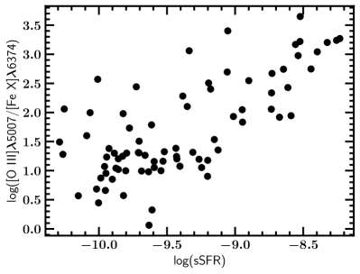
Figure 13: The reddening-corrected [O III]$\lambda$5007/[Fe X]$\lambda$6374 line ratio vs. the sSFR for the [Fe X]$\lambda$6374-emitting galaxies. The ratio increases with sSFR, which could indicate the star formation is hiding the signature TDE-like line ratio.

7.2 Biases in AGN Selection Methods and the Effect on the [Fe X]-selected Sample of Dwarf Galaxies

The AGN selection techniques explored in this work focus on distinct regions of the electromagnetic spectrum that probe emission from different parts of an AGN. Most of these techniques assume that the accretion disk is well-explained by the radiatively efficient, geometrically thin, optically thick model first presented by Shakura & Sunyaev (1976). In this model, the disk will produce optical and UV photons that will inverse Compton scatter away from the disk to produce hard X-ray emission in the hot, tenuous coronal region (Liang & Nolan, 1984; Haardt & Maraschi, 1991) which photoionizes the observed [Fe X]$\lambda$6374 and other coronal-line emission (e.g., Nussbaumer & Osterbrock, 1970; Korista & Ferland, 1989; Oliva et al., 1994; Pier & Voit, 1995). Gas within the broad line region (BLR; 10–100 light days in Seyfert 1 galaxies) will have high Doppler motions, creating broad-line emission. Meanwhile the narrow line region (NLR) is produced by gas farther away from the central BH (100–300 pc) creating narrower emission-line widths (Netzer, 2013). The emission in the narrow-line region will also be photoionized by the central engine, creating the characteristic AGN-like emission seen in the VO87 (BPT-style), NIR and He II/H$\beta$ diagrams (Veilleux & Osterbrock, 1987; Baldwin et al., 1981; Kewley et al., 2006; Osterbrock et al., 1992; Sartori et al., 2015). Additionally, AGN jets produce synchrotron emission in the radio that is not affected by dust attenuation and emitted at some level by almost all AGN (Ho, 2008). Finally, almost all emission from AGNs is observed to vary on characteristic timescales related to the processes from which the emission is created (e.g., Ulrich et al., 1997).

Conversely, radiatively inefficient accretion flows (RIAFs; Narayan & Yi, 1995; Blandford & Begelman, 1999) have very different accretion-disk structures. The accretion rate in RIAFs is so low ($L_{\rm bol}/L_{\rm Edd}\lesssim 10^{-2}$) that at a certain transition radius, $R_{t}$, the collisional cooling timescale equals the accretion timescale. Outside of $R_{t}$ the accretion disk is geometrically thin and optical thick. However inside $R_{t}$ the disk becomes geometrically thick and optical thin. In this regime, the electrons are cooled by bremsstrahlung, synchrotron and Compton up-scattering while the ions remain at the virial temperature. This change in accretion-disk structure could remove some of the more traditional AGN-like narrow-line ratios and broad H$\alpha$ emission (Ho, 2008; Trump et al., 2011) and are predicted to have strong radio outflows (Meier, 2001; Fender & Belloni, 2004). These radio outflows can create radiative winds that collisionally excite the observed [Fe X]$\lambda$6374 emission seen in RIAFs (e.g., Wilson & Raymond, 1999). This would result in a predominantly wind-driven energy budget, which is expected as the accretion rate decreases (Meléndez et al., 2008; Diamond-Stanic et al., 2009).

The difference between these two accretion flows typically seen in AGNs will affect the viability of the various AGN detection methods explored here. For example, the optical spectroscopic tests such as the narrow-line diagnostic diagrams, He II/H$\beta$ line ratio and broad H$\alpha$ emission can easily miss AGNs with RIAFs (Ho, 2008; Trump et al., 2011) or radiatively efficient AGNs that reside within host galaxies with even modest star formation rates (e.g., Moran et al., 2002). While X-ray and radio detections are relatively cleaner sources of AGN activity, the signal could be comparable to that of the ambient star formation in the host galaxy which can also effectively hide the AGN signal (e.g., Reines et al., 2020; Latimer et al., 2021). Finally, AGN variability is rarely seen in AGNs with RIAFs (Trump et al., 2009), which could lead to a systematic bias towards radiatively efficient central engines. These effects could explain why many of our [Fe X]-selected AGN candidates do not show other traditional AGN indicators.

The two most recent discoveries of AGN-related [Fe X]$\lambda$6374 emission in dwarf galaxies (e.g., Molina et al., 2021; Kimbro et al., 2021) used multi-wavelength data to identify a RIAF as the most likely BH accretion structure. We therefore anticipate that some fraction of our objects are also likely AGNs with RIAFs, which are biased against in most of the AGN selection techniques used in this work. Given RIAFs are predicted to have strong radio outflows, searching for radio emission is clearly the preferred AGN detection technique. While only a few objects in our sample have strong radio detections in FIRST, many AGNs even in the low-redshift universe, do not produce enough radio continuum to be detected by the FIRST survey (Condon et al., 2019). We also included data from the first epoch of VLASS, which has significantly better angular resolution but a sensitivity threshold similar to that of FIRST (0.12 mJy vs. 0.15 mJy). Thus dedicated radio and X-ray follow-up could help determine if weakly accreting BHs with RIAFs are present in these objects.

Meanwhile, some of the objects in this sample, such as NSA 256802, clearly harbor radiatively efficient AGNs. Therefore the corona is likely photoionizing the observed [Fe X]$\lambda$6374 emission in these galaxies. We do note that NSA 256802 is particularly unique in this sample as it is the only object that is AGN-like using the BPT-like narrow-line diagrams. However, optical AGN signatures can easily be hidden by a modest amount of star formation in the host galaxy (Moran et al., 2002). The galaxies in our sample are very blue and have substantial mass-specific SFRs, indicating a high level of star formation which can easily dilute the more traditional narrow-line diagnostic indicators (Cann et al., 2019; Trump et al., 2015). Therefore, it is also possible that a significant fraction of these galaxies harbor thin-disk AGNs. Spectroscopy with the James Webb Space Telescope (JWST) would be useful for identifying near-IR coronal lines that can be used to identify AGN photoionization in radiatively efficient BHs (e.g., Satyapal et al., 2021; Cann et al., 2018).

7.3 Comparison to Optical and Radio-Selected Samples of AGNs in Dwarf Galaxies

We first compare our objects to the AGN and composite samples from Reines et al. (2013) that were identified using the [O III]/H$\beta$ vs. [N II]/H$\alpha$ diagram. As the Reines et al. (2013) objects are luminous enough to be detected in the 3″ SDSS aperture, and exhibit narrow-line ratios consistent with AGN activity, they are likely BHs with radiatively efficient flows. Indeed, the broad-line AGNs and composites in Reines et al. (2013) have Eddington ratios spanning $\sim 0.1$–50%, comparable to high-redshift, massive broad-line quasars (Baldassare et al., 2017). Therefore, they represent the most energetic, most luminous end of the dwarf galaxy AGN population.

In the work presented here, we used the updated NSA v1_0_1 catalog, which has a 100% overlap with the v0_1_2 catalog used by Reines et al. (2013). Interestingly, while 136 objects were detected as either AGN or composite galaxies by Reines et al., only two of those objects are included in our [Fe X] sample. When we compare the properties of our sample to the Reines et al. (2013) AGN and composite samples as shown in Figure 4, we find that a majority our sample covers the lower-mass, bluer region of the $g-r$ vs. $M_{*}$ diagram. In fact, K–S two sample tests comparing the $g-r$ colors and mass between the [Fe X]$\lambda$6374-selected AGN candidate sample and the AGN and composite samples from Reines et al. (2013) show that they are statistically distinct at the 99% confidence level.

The statistical difference seen in the Reines et al. (2013) AGNs/composites and the [Fe X]$\lambda$6374-selected AGNs presented here could be a result of various phenomena including: (1) AGNs with [Fe X]$\lambda$6374 emission in dwarf galaxies are biased towards a RIAF-like engines, (2) the [Fe X]$\lambda$6374 emission line is significantly harder to produce via stellar emission than [N II], allowing us to detect AGNs in bluer galaxies with more star formation, and (3) a combination of (1) and (2).

We also compared our sample to the radio-selected AGN candidates in Reines et al. (2020). Similar to our [Fe X]-selected sample, many of the Reines et al. (2020) objects did not have obvious AGN-like emission in their SDSS spectra, even when the radio source overlapped with the SDSS fiber (although many had enhanced [O I]/H$\alpha$). We find our sample has a similar distribution in color and mass to the Reines et al. (2020) AGN candidates, as seen in Figure 4.

At first glance, once could conclude that the similarity between the two samples may indicate the presence of radio activity in the [Fe X]$\lambda$6374-selected sample. However, it may just be that both of these samples access part of the dwarf galaxy population that is not accessible using traditional optical diagnostics with SDSS spectroscopy as desmonstrated by Figure 4. Thus [Fe X] surveys provide a pathway for finding BHs in a dwarf-galaxy population that is notoriously difficult to explore with other detection methods.

8 Summary and Conclusions

In this work, we present the first systematic search for [Fe X]$\lambda$6374-selected massive BHs in dwarf galaxies. Our main results are as follows:

1. We identified [Fe X]$\lambda$6374 emission in the SDSS single-fiber spectroscopy of 81 dwarf galaxies. The [Fe X]$\lambda$6374 luminosities are in the range $10^{36\mbox{--}39}$ erg s^-1, with a median of $1.6\times 10^{38}$ erg s^-1, and indicate massive BHs are likely present in the majority of galaxies in our sample. AGNs and/or TDEs are the most likely origin of the [Fe X]$\lambda$6374 emission.

2. The [Fe X]$\lambda$6374 luminosities are sufficiently high to exclude stellar origins of the emission (e.g., Wolf-Rayet stars, planetary nebula, supernovae) in most of our sample galaxies. There are a couple of known luminous Type IIn SNe with $L_{[\rm FeX]}\lesssim 2\times 10^{37}$ erg s^-1; however, a majority of our objects have [Fe X] luminosities well above that value. Furthermore, we expect at most 8 Type IIn SNe in our sample, indicating that the [Fe X] emission in most of these objects is driven by massive BH activity.

3. [Fe X]$\lambda$6374 emission can be produced by AGN photoionization or shocks from AGN jets. Given the results of previous studies of BHs in dwarf galaxies with strong [Fe X]$\lambda$6374 emission (Molina et al., 2021; Kimbro et al., 2021), we expect some of the AGNs in this work will also be weakly-accreting BHs, potentially with RIAF structures. Follow-up observations, particularly at X-ray and radio wavelengths, would help us assess the nature of the accretion flows around the BHs in these dwarf galaxies.

4. We searched for additional AGN indicators in our sample of [Fe X]-detected dwarf galaxies using optical spectroscopy and optical variability, as well as existing X-ray and radio observations. While 51% of the objects have multiple AGN signatures, many galaxies in our sample are only selected as active BHs via their high [Fe X]$\lambda$6374 luminosity.

5. The objects in our sample also have [Fe X] luminosities and estimated BH masses consistent with that seen in some TDEs. While our galaxies do not show other traditional TDE indicators (i.e., [O III$]/[\hbox{Fe\,{\scriptsize X}}]\sim 1$), it is possible that these signatures are being diluted by high levels of star formation. One galaxy in our sample, NSA 427201, is a particularly strong TDE candidate, demonstrating that [Fe X] could potentially trace a population of TDEs in star-forming dwarfs.

6. Overall, the galaxies in our sample exhibit bluer colors and lower stellar masses than the traditional BPT-selected AGN (Reines et al., 2013) in dwarf galaxies, indicating that [Fe X]$\lambda$6374 searches can identify BH activity in galaxies with higher levels of ongoing star formation.

We conclude that [Fe X]$\lambda$6374 is a powerful new tool to search for the elusive low-mass AGN, and potentially TDE, populations in dwarf galaxies. Furthermore, [Fe X] searches can be used to construct samples of candidate NIR coronal-line emitting galaxies to observe with JWST (e.g., Cann et al., 2018). Similar to radio searches, [Fe X]$\lambda$6374 searches can detect BH activity in lower-mass galaxies with significant star formation that are difficult to find in traditional optical surveys. We also demonstrate that this work can be completed using single-epoch optical surveys, which allows for efficient searches for BH activity in dwarf galaxies. Therefore, BHs detected via [Fe X]$\lambda$6374 emission can help constrain the low-mass end of the BH population in dwarf galaxies and shed light on the origin of BH seeds. (e.g., Reines & Comastri, 2016; Greene et al., 2020).

Appendix A Galaxy Images and [Fe X]$\lambda$6374 Spectra

The DESI Legacy Imaging Survey images of each [Fe X]$\lambda$6374-emitting galaxy along with the [Fe X] emission-line fit are shown in Figures 14–16. The [Fe X] fitting process is described in Section 2.

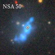
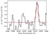
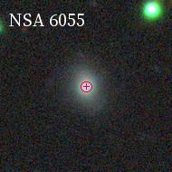
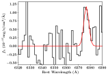
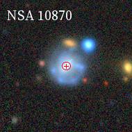
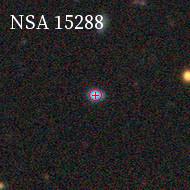
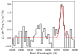
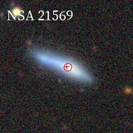
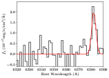
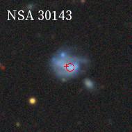
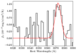
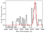
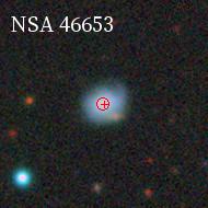
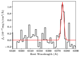
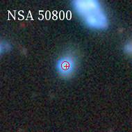
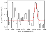
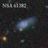
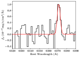
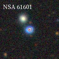
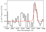
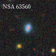
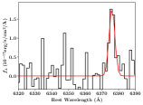
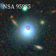
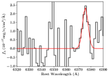
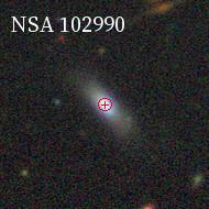
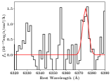
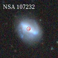
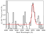
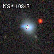
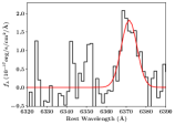
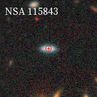
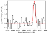
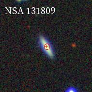
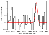
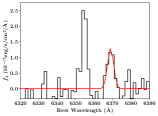
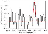
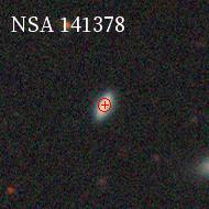
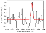
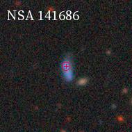
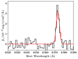
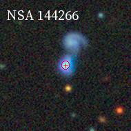
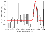
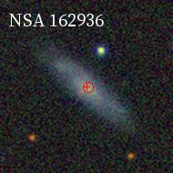
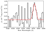
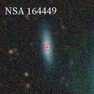
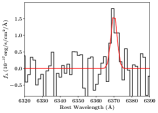
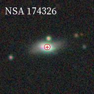
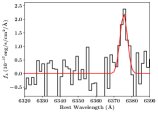
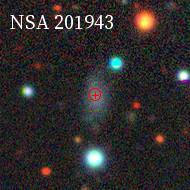
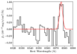
Figure 14: Pairs of the [Fe X]$\lambda$6374-emitting dwarf galaxy DESI Legacy Imaging Survey SkyViewer $grz$-band images and the fit to the [Fe X]$\lambda$6374 emission line using the [O I] and continuum-subtracted spectrum. For each pair, the image is on the left and the spectral fit is on the right. In each of the SkyViewer images, the position of the galaxy nucleus as defined by the NSA is shown by the red cross, and the position of the SDSS 3″ spectroscopic fiber is shown by the red circle. For each SDSS spectral fit, the data are shown in black and the [Fe X]$\lambda$6374 emission-line model is overplotted in red.

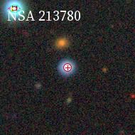
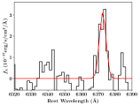
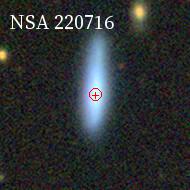
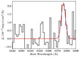
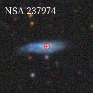
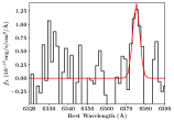
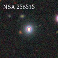
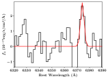
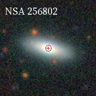
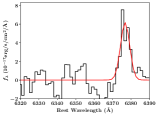
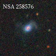
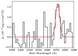
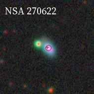
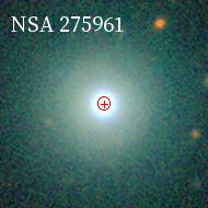
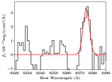
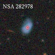
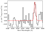
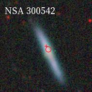
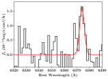
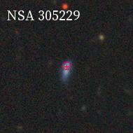
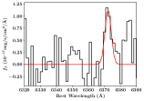
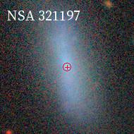
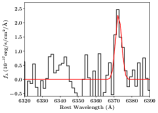
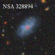
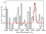
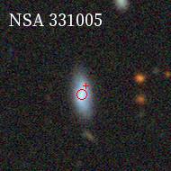
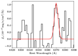
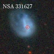
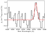
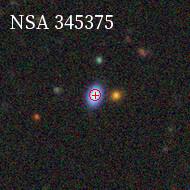
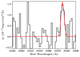
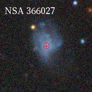
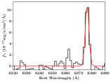
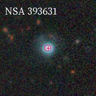
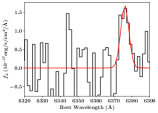
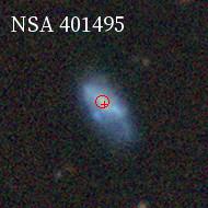
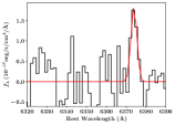
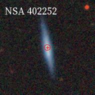
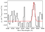
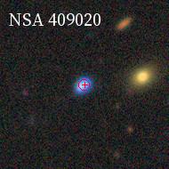
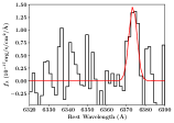
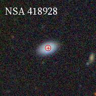
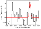
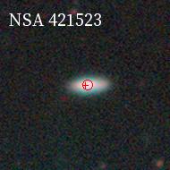
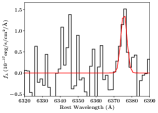
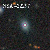
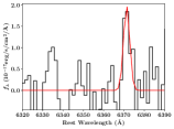
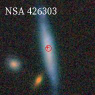
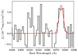
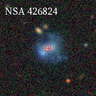
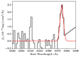
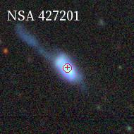
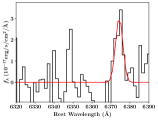
Figure 15: Same as Figure 14.

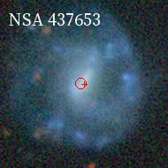
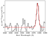
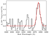
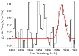
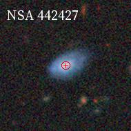
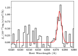
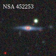
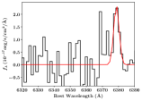
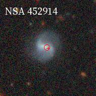
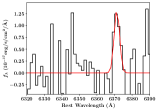
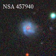
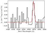
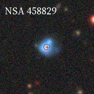
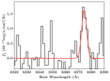
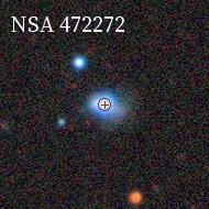
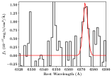
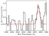
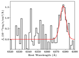
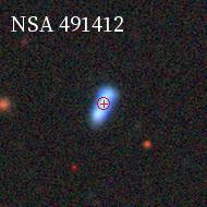
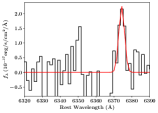
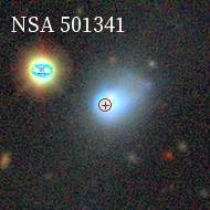
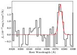
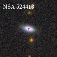
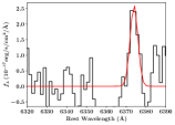
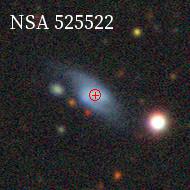
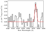
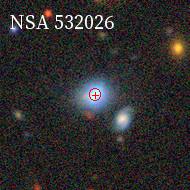
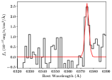
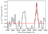
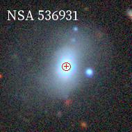
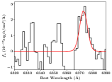
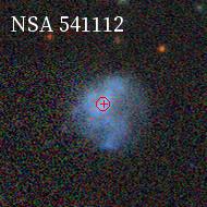
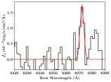
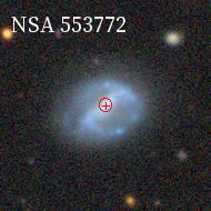
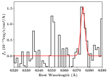
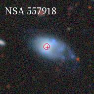
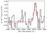
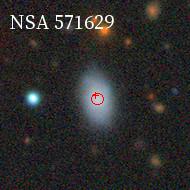
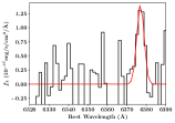
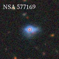
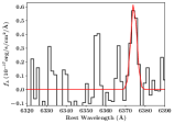
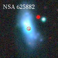
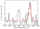
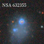
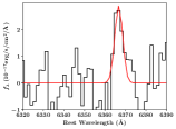
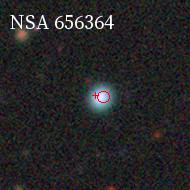
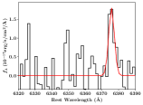
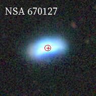
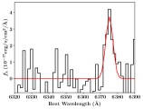
Figure 16: Same as Figure 14.

Appendix B Notes on Individual Objects in Previous Studies

• NSA 50: This galaxy is a known He II emitting galaxy (Shirazi & Brinchmann, 2012), and the high-resolution VLA data taken by Reines et al. (2020) could not rule out star formation as the cause of the observed radio emission. We confirm the result from Reines et al. (2020) using the FIRST survey radio detections in this work. Additionally, we could not rule out high-mass XRBs as the cause of the observed X-ray emission. Furthermore, the [Fe X] emission seen in the SDSS spectrum is consistent with that of SN2005ip. We do note that the He II/H$\beta$ ratio indicates the presence of an AGN, and this galaxy appeared Seyfert-like in the [O III]/H$\beta$ vs. [S II]/H$\alpha$ and [O I]/H$\alpha$ diagrams. Given the low [Fe X] detection, it is unclear whether the optical emission is driven by AGN activity or a very energetic Type IIn SNe driving strong shocks into the circumstellar medium.

• NSA 95985: This galaxy was designated as an X-ray AGN candidate by Birchall et al. (2020). While the detected [Fe X] emission is consistent with that seen in SN2005ip, the object is Seyfert-like in both the [O III]/H$\beta$ vs. [S II]/H$\alpha$ and [O I]/H$\alpha$ diagrams.

• NSA 131809: This galaxy was presented as a variable AGN candidate by Baldassare et al. (2020). In this work, we find that the observed [Fe X]$\lambda$6374 emission is about 7 times stronger than that seen in the Type IIn supernova SN2005ip, providing additional support for an AGN.

• NSA 256802: This galaxy was designated as a broad-line AGN by (Reines et al., 2013, their ID 20). We recover this designation, and note that this is the only AGN object from Reines et al. (2013) that overlaps with our sample. Given the strong X-ray emission shown in Figure 11 as well as the prominent broad H$\alpha$ emission, we conclude the [Fe X] emission seen in this object is likely produced by gas photoionized by a radiatively efficient accretion disk.

• NSA 275961: This galaxy was designated as a composite object by Reines et al. (2013, their ID 105). In this work, we recover the designation of composite using the VO87 diagrams, and find that the object appears AGN-like via the He II/H$\beta$ ratio and the [S II]/H$\alpha$ vs. [O II]$\lambda\lambda$7320,7330/H$\alpha$ diagram. Additionally, the archival Chandra data indicate that this object is also AGN-like (see Figure 11).

• NSA 300542: This galaxy was labeled as a SNe candidate by Reines et al. (2013) via the detection of a P Cygni profile in H$\alpha$ (NSAv0 61339 in their work). However, the P Cygni profile was very subtle in this object, as shown in Figure 7 in Reines et al. (2013). In this work, we found that NSA 300542 appears Seyfert-like in the [O III]/H$\beta$ vs. [S II]/H$\alpha$ and [O I]/H$\alpha$ diagrams as well as the [S II]/H$\alpha$ vs. [O II]$\lambda\lambda$7320,7330/H$\alpha$ diagram. Additionally, the [Fe X]$\lambda$6374 emission is about 6 times stronger than SN2005ip.

• NSA 427201: This galaxy was labelled as a star-forming galaxy with broad H$\alpha$ by Reines et al. (2013, their object N), and not detected in the radio by Reines et al. (2020). We recover the broad component first seen by Reines et al. (2013), and also find that the observed radio emission in both VLASS and FIRST cannot be explained by stellar processes. Additionally, the [Fe X]$\lambda$6374 emission seen in this object is $\sim 19$ times higher than that seen in SN2005ip. Given the lack of broad-line emission seen by Baldassare et al. (2016) and radio emission seen by Reines et al. (2020), we conclude this object is a TDE candidate. See Section 7.1 for a more thorough discussion.

• NSA 533731: This galaxy is also known as Mrk 709S, is in a pair of interacting galaxies first studied in depth by Reines et al. (2014), and is one of the two objects that inspired this work. Mrk 709S was confirmed to harbor a LLAGN with a RIAF engine and strong out-flowing winds by Kimbro et al. (2021). In this work, we find that the observed [Fe X]$\lambda$6374 emission is almost 23 times higher than that seen in SN2005ip, and has an additional marker of AGN activity via strong radio emission seen in both the FIRST and VLASS surveys.

References

- Ahumada et al. (2020) Ahumada, R., Prieto, C. A., Almeida, A., et al. 2020, ApJS, 249, 3
- Allende Prieto et al. (2001) Allende Prieto, C., Lambert, D. L., & Asplund, M. 2001, ApJ, 556, L63
- Anglés-Alcázar et al. (2017) Anglés-Alcázar, D., Faucher-Giguère, C.-A., Quataert, E., et al. 2017, MNRAS, 472, L109
- Astropy Collaboration et al. (2013) Astropy Collaboration, Robitaille, T. P., Tollerud, E. J., et al. 2013, A&A, 558, A33
- Astropy Collaboration et al. (2018) Astropy Collaboration, Price-Whelan, A. M., Sipőcz, B. M., et al. 2018, AJ, 156, 123
- Aversa et al. (2011) Aversa, A. G., Johnson, K. E., Brogan, C. L., Goss, W. M., & Pisano, D. J. 2011, AJ, 141, 125
- Baldassare et al. (2018) Baldassare, V. F., Geha, M., & Greene, J. 2018, ApJ, 868, 152
- Baldassare et al. (2020) —. 2020, ApJ, 896, 10
- Baldassare et al. (2017) Baldassare, V. F., Reines, A. E., Gallo, E., & Greene, J. E. 2017, ApJ, 836, 20
- Baldassare et al. (2016) Baldassare, V. F., Reines, A. E., Gallo, E., et al. 2016, ApJ, 829, 57
- Baldwin et al. (1981) Baldwin, J. A., Phillips, M. M., & Terlevich, R. 1981, PASP, 93, 5
- Becker et al. (1995) Becker, R. H., White, R. L., & Helfand, D. J. 1995, ApJ, 450, 559
- Begelman et al. (2006) Begelman, M. C., Volonteri, M., & Rees, M. J. 2006, MNRAS, 370, 289
- Bellovary et al. (2011) Bellovary, J., Volonteri, M., Governato, F., et al. 2011, ApJ, 742, 13
- Birchall et al. (2020) Birchall, K. L., Watson, M. G., & Aird, J. 2020, MNRAS, 492, 2268
- Blandford & Begelman (1999) Blandford, R. D., & Begelman, M. C. 1999, MNRAS, 303, L1
- Blanton et al. (2011) Blanton, M. R., Kazin, E., Muna, D., Weaver, B. A., & Price-Whelan, A. 2011, AJ, 142, 31
- Blanton et al. (2017) Blanton, M. R., Bershady, M. A., Abolfathi, B., et al. 2017, AJ, 154, 28
- Bode & Evans (2008) Bode, M. F., & Evans, A. 2008, Classical Novae, Vol. 43
- Bohn et al. (2021) Bohn, T., Canalizo, G., Veilleux, S., & Liu, W. 2021, ApJ, 911, 70
- Bolton et al. (2012) Bolton, A. S., Schlegel, D. J., Aubourg, É., et al. 2012, AJ, 144, 144
- Bond et al. (1984) Bond, J. R., Arnett, W. D., & Carr, B. J. 1984, ApJ, 280, 825
- Bromm & Yoshida (2011) Bromm, V., & Yoshida, N. 2011, ARA&A, 49, 373
- Bruzual & Charlot (2003) Bruzual, G., & Charlot, S. 2003, MNRAS, 344, 1000
- Bundy et al. (2015) Bundy, K., Bershady, M. A., Law, D. R., et al. 2015, ApJ, 798, 7
- Butler & Bloom (2011) Butler, N. R., & Bloom, J. S. 2011, AJ, 141, 93
- Cann et al. (2019) Cann, J. M., Satyapal, S., Abel, N. P., et al. 2019, ApJ, 870, L2
- Cann et al. (2018) —. 2018, ApJ, 861, 142
- Cappellari (2017) Cappellari, M. 2017, MNRAS, 466, 798
- Cerqueira-Campos et al. (2021) Cerqueira-Campos, F. C., Rodríguez-Ardila, A., Riffel, R., et al. 2021, MNRAS, 500, 2666
- Choi et al. (2015) Choi, J.-H., Shlosman, I., & Begelman, M. C. 2015, MNRAS, 450, 4411
- Chomiuk & Wilcots (2009) Chomiuk, L., & Wilcots, E. M. 2009, ApJ, 703, 370
- Coe et al. (2021) Coe, M. J., Kennea, J. A., Evans, P. A., et al. 2021, MNRAS, 504, 1398
- Condon (1992) Condon, J. J. 1992, ARA&A, 30, 575
- Condon et al. (2019) Condon, J. J., Matthews, A. M., & Broderick, J. J. 2019, ApJ, 872, 148
- Danehkar et al. (2021) Danehkar, A., Oey, M. S., & Gray, W. J. 2021, arXiv e-prints, arXiv:2106.10854
- Davies et al. (2011) Davies, M. B., Miller, M. C., & Bellovary, J. M. 2011, ApJ, 740, L42
- Dawson et al. (2013) Dawson, K. S., Schlegel, D. J., Ahn, C. P., et al. 2013, AJ, 145, 10
- Devecchi & Volonteri (2009) Devecchi, B., & Volonteri, M. 2009, ApJ, 694, 302
- Dey et al. (2019) Dey, A., Schlegel, D. J., Lang, D., et al. 2019, AJ, 157, 168
- Diamond-Stanic et al. (2009) Diamond-Stanic, A. M., Rieke, G. H., & Rigby, J. R. 2009, ApJ, 698, 623
- Dickey & Lockman (1990) Dickey, J. M., & Lockman, F. J. 1990, ARA&A, 28, 215
- Dong et al. (2012) Dong, R., Greene, J. E., & Ho, L. C. 2012, ApJ, 761, 73
- Dopita et al. (1997) Dopita, M. A., Koratkar, A. P., Allen, M. G., et al. 1997, ApJ, 490, 202
- Fender & Belloni (2004) Fender, R., & Belloni, T. 2004, ARA&A, 42, 317
- Fernandes et al. (2004) Fernandes, I. F., de Carvalho, R., Contini, T., & Gal, R. R. 2004, MNRAS, 355, 728
- Filippenko (1997) Filippenko, A. V. 1997, ARA&A, 35, 309
- Filippenko & Sargent (1988) Filippenko, A. V., & Sargent, W. L. W. 1988, ApJ, 324, 134
- Filippenko & Sargent (1989) —. 1989, ApJ, 342, L11
- Fruscione et al. (2006) Fruscione, A., McDowell, J. C., Allen, G. E., et al. 2006, in Society of Photo-Optical Instrumentation Engineers (SPIE) Conference Series, Vol. 6270, Society of Photo-Optical Instrumentation Engineers (SPIE) Conference Series, 1
- Gehrels (1986) Gehrels, N. 1986, ApJ, 303, 336
- Gelbord et al. (2009) Gelbord, J. M., Mullaney, J. R., & Ward, M. J. 2009, MNRAS, 397, 172
- Gilfanov (2004) Gilfanov, M. 2004, Monthly Notices of the Royal Astronomical Society, 349, 146
- Ginsburg & Mirocha (2011) Ginsburg, A., & Mirocha, J. 2011, PySpecKit: Python Spectroscopic Toolkit
- Gordon et al. (2020) Gordon, Y. A., Boyce, M. M., O’Dea, C. P., et al. 2020, Research Notes of the American Astronomical Society, 4, 175
- Goulding & Alexander (2009) Goulding, A. D., & Alexander, D. M. 2009, MNRAS, 398, 1165
- Graur et al. (2015) Graur, O., Bianco, F. B., & Modjaz, M. 2015, MNRAS, 450, 905
- Greene & Ho (2004) Greene, J. E., & Ho, L. C. 2004, ApJ, 610, 722
- Greene et al. (2020) Greene, J. E., Strader, J., & Ho, L. C. 2020, ARA&A, 58, 257
- Grimm et al. (2003) Grimm, H.-J., Gilfanov, M., & Sunyaev, R. 2003, Monthly Notices of the Royal Astronomical Society, 339, 793
- Groves et al. (2006) Groves, B. A., Heckman, T. M., & Kauffmann, G. 2006, MNRAS, 371, 1559
- Gunn et al. (2006) Gunn, J. E., Siegmund, W. A., Mannery, E. J., et al. 2006, AJ, 131, 2332
- Haardt & Maraschi (1991) Haardt, F., & Maraschi, L. 1991, ApJ, 380, L51
- Habouzit et al. (2017) Habouzit, M., Volonteri, M., & Dubois, Y. 2017, MNRAS, 468, 3935
- Hainline et al. (2016) Hainline, K. N., Reines, A. E., Greene, J. E., & Stern, D. 2016, ApJ, 832, 119
- Hao et al. (2011) Hao, C.-N., Kennicutt, R. C., Johnson, B. D., et al. 2011, The Astrophysical Journal, 741, 124
- He et al. (2019) He, L., Wang, S., Liu, J., et al. 2019, ApJ, 871, 193
- Heckman et al. (2001) Heckman, T. M., Sembach, K. R., Meurer, G. R., et al. 2001, ApJ, 554, 1021
- Heger & Woosley (2002) Heger, A., & Woosley, S. E. 2002, ApJ, 567, 532
- Hickox & Alexander (2018) Hickox, R. C., & Alexander, D. M. 2018, ARA&A, 56, 625
- Ho (2008) Ho, L. C. 2008, ARA&A, 46, 475
- Ho (2009) —. 2009, ApJ, 699, 626
- Ho et al. (1997) Ho, L. C., Filippenko, A. V., Sargent, W. L. W., & Peng, C. Y. 1997, ApJS, 112, 391
- Hong et al. (2005) Hong, J., van den Berg, M., Schlegel, E. M., et al. 2005, ApJ, 635, 907
- Hunter (2007) Hunter, J. D. 2007, Computing in Science Engineering, 9, 90
- Jarrett et al. (2011) Jarrett, T. H., Cohen, M., Masci, F., et al. 2011, ApJ, 735, 112
- Jarrett et al. (2013) Jarrett, T. H., Masci, F., Tsai, C. W., et al. 2013, The Astronomical Journal, 145, 6
- Johnson et al. (2009) Johnson, K. E., Hunt, L. K., & Reines, A. E. 2009, AJ, 137, 3788
- Karthick et al. (2014) Karthick, M. C., López-Sánchez, Á. R., Sahu, D. K., Sanwal, B. B., & Bisht, S. 2014, MNRAS, 439, 157
- Kauffmann et al. (2003) Kauffmann, G., Heckman, T. M., Tremonti, C., et al. 2003, MNRAS, 346, 1055
- Kehrig et al. (2018) Kehrig, C., Vílchez, J. M., Guerrero, M. A., et al. 2018, MNRAS, 480, 1081
- Kelly et al. (2009) Kelly, B. C., Bechtold, J., & Siemiginowska, A. 2009, ApJ, 698, 895
- Kennicutt (1998) Kennicutt, Robert C., J. 1998, ARA&A, 36, 189
- Kennicutt & Evans (2012) Kennicutt, R. C., & Evans, N. J. 2012, ARA&A, 50, 531
- Kepley et al. (2014) Kepley, A. A., Reines, A. E., Johnson, K. E., & Walker, L. M. 2014, AJ, 147, 43
- Kewley et al. (2006) Kewley, L. J., Groves, B., Kauffmann, G., & Heckman, T. 2006, MNRAS, 372, 961
- Kewley et al. (2019) Kewley, L. J., Nicholls, D. C., & Sutherland, R. S. 2019, ARA&A, 57, 511
- Kimbro et al. (2021) Kimbro, E., Reines, A. E., Molina, M., Deller, A. T., & Stern, D. 2021, arXiv e-prints, arXiv:2103.05655
- Komossa et al. (2008) Komossa, S., Zhou, H., Wang, T., et al. 2008, ApJ, 678, L13
- Komossa et al. (2009) Komossa, S., Zhou, H., Rau, A., et al. 2009, ApJ, 701, 105
- Korista & Ferland (1989) Korista, K. T., & Ferland, G. J. 1989, ApJ, 343, 678
- Kormendy & Ho (2013) Kormendy, J., & Ho, L. C. 2013, ARA&A, 51, 511
- Kormendy & Richstone (1995) Kormendy, J., & Richstone, D. 1995, ARA&A, 33, 581
- Kraft et al. (1991) Kraft, R. P., Burrows, D. N., & Nousek, J. A. 1991, ApJ, 374, 344
- Lacy et al. (2020) Lacy, M., Baum, S. A., Chandler, C. J., et al. 2020, PASP, 132, 035001
- Lamperti et al. (2017) Lamperti, I., Koss, M., Trakhtenbrot, B., et al. 2017, MNRAS, 467, 540
- Latimer et al. (2021) Latimer, C. J., Reines, A. E., Hainline, K. N., Greene, J. E., & Stern, D. 2021, arXiv e-prints, arXiv:2105.05876
- Law et al. (2009) Law, N. M., Kulkarni, S. R., Dekany, R. G., et al. 2009, PASP, 121, 1395
- Leaman et al. (2011) Leaman, J., Li, W., Chornock, R., & Filippenko, A. V. 2011, MNRAS, 412, 1419
- Lehmer et al. (2021) Lehmer, B. D., Eufrasio, R. T., Basu-Zych, A., et al. 2021, ApJ, 907, 17
- Liang & Nolan (1984) Liang, E. P., & Nolan, P. L. 1984, Space Sci. Rev., 38, 353
- Lintott et al. (2011) Lintott, C., Schawinski, K., Bamford, S., et al. 2011, MNRAS, 410, 166
- Lodato & Natarajan (2006) Lodato, G., & Natarajan, P. 2006, MNRAS, 371, 1813
- Loeb & Rasio (1994) Loeb, A., & Rasio, F. A. 1994, ApJ, 432, 52
- Lupi et al. (2014) Lupi, A., Colpi, M., Devecchi, B., Galanti, G., & Volonteri, M. 2014, MNRAS, 442, 3616
- Lynch et al. (2007) Lynch, D. K., Rudy, R. J., Prater, T. R., et al. 2007, IAU Circ., 8906, 1
- MacLeod et al. (2010) MacLeod, C. L., Ivezić, Ž., Kochanek, C. S., et al. 2010, ApJ, 721, 1014
- Mateos et al. (2012) Mateos, S., Alonso-Herrero, A., Carrera, F. J., et al. 2012, MNRAS, 426, 3271
- McGaugh et al. (2017) McGaugh, S. S., Schombert, J. M., & Lelli, F. 2017, ApJ, 851, 22
- Meier (2001) Meier, D. L. 2001, ApJ, 548, L9
- Meléndez et al. (2008) Meléndez, M., Kraemer, S. B., Armentrout, B. K., et al. 2008, ApJ, 682, 94
- Molina et al. (2018) Molina, M., Eracleous, M., Barth, A. J., et al. 2018, ApJ, 864, 90
- Molina et al. (2021) Molina, M., Reines, A. E., Greene, J. E., Darling, J., & Condon, J. J. 2021, ApJ, 910, 5
- Moran et al. (2002) Moran, E. C., Filippenko, A. V., & Chornock, R. 2002, ApJ, 579, L71
- Moretti et al. (2003) Moretti, A., Campana, S., Lazzati, D., & Tagliaferri, G. 2003, ApJ, 588, 696
- Moro-Martín et al. (2001) Moro-Martín, A., Garnavich, P. M., & Noriega-Crespo, A. 2001, AJ, 121, 1636
- Murayama & Taniguchi (1998) Murayama, T., & Taniguchi, Y. 1998, ApJ, 503, L115
- Nagao et al. (2000) Nagao, T., Taniguchi, Y., & Murayama, T. 2000, AJ, 119, 2605
- Narayan & Yi (1995) Narayan, R., & Yi, I. 1995, ApJ, 452, 710
- Natarajan (2014) Natarajan, P. 2014, General Relativity and Gravitation, 46, 1702
- Negus et al. (2021) Negus, J., Comerford, J. M., Müller Sánchez, F., et al. 2021, arXiv e-prints, arXiv:2107.11631
- Netzer (2013) Netzer, H. 2013, The Physics and Evolution of Active Galactic Nuclei
- Nussbaumer & Osterbrock (1970) Nussbaumer, H., & Osterbrock, D. E. 1970, ApJ, 161, 811
- Oetken (1977) Oetken, L. 1977, Astronomische Nachrichten, 298, 187
- Oliva et al. (1994) Oliva, E., Salvati, M., Moorwood, A. F. M., & Marconi, A. 1994, A&A, 288, 457
- Osterbrock et al. (1992) Osterbrock, D. E., Tran, H. D., & Veilleux, S. 1992, ApJ, 389, 196
- Park et al. (2006) Park, T., Kashyap, V. L., Siemiginowska, A., et al. 2006, ApJ, 652, 610
- Penston et al. (1984) Penston, M. V., Fosbury, R. A. E., Boksenberg, A., Ward, M. J., & Wilson, A. S. 1984, MNRAS, 208, 347
- Pettini & Pagel (2004) Pettini, M., & Pagel, B. E. J. 2004, MNRAS, 348, L59
- Pier & Voit (1995) Pier, E. A., & Voit, G. M. 1995, ApJ, 450, 628
- Portegies Zwart et al. (2004) Portegies Zwart, S. F., Baumgardt, H., Hut, P., Makino, J., & McMillan, S. L. W. 2004, Nature, 428, 724
- Pottasch et al. (2009) Pottasch, S. R., Bernard-Salas, J., & Roellig, T. L. 2009, A&A, 499, 249
- Prieto et al. (2002) Prieto, M. A., Pérez García, A. M., & Rodríguez Espinosa, J. M. 2002, MNRAS, 329, 309
- Prieto & Viegas (2000) Prieto, M. A., & Viegas, S. M. 2000, ApJ, 532, 238
- Rau et al. (2009) Rau, A., Kulkarni, S. R., Law, N. M., et al. 2009, PASP, 121, 1334
- Reines & Comastri (2016) Reines, A. E., & Comastri, A. 2016, PASA, 33, e054
- Reines et al. (2020) Reines, A. E., Condon, J. J., Darling, J., & Greene, J. E. 2020, ApJ, 888, 36
- Reines et al. (2013) Reines, A. E., Greene, J. E., & Geha, M. 2013, ApJ, 775, 116
- Reines et al. (2008) Reines, A. E., Johnson, K. E., & Goss, W. M. 2008, AJ, 135, 2222
- Reines et al. (2014) Reines, A. E., Plotkin, R. M., Russell, T. D., et al. 2014, ApJ, 787, L30
- Reines & Volonteri (2015) Reines, A. E., & Volonteri, M. 2015, ApJ, 813, 82
- Reunanen et al. (2003) Reunanen, J., Kotilainen, J. K., & Prieto, M. A. 2003, MNRAS, 343, 192
- Riffel et al. (2006) Riffel, R., Rodríguez-Ardila, A., & Pastoriza, M. G. 2006, A&A, 457, 61
- Rosen et al. (2016) Rosen, S. R., Webb, N. A., Watson, M. G., et al. 2016, A&A, 590, A1
- Rudy et al. (2021) Rudy, R. J., Subasavage, J. P., Mauerhan, J. C., et al. 2021, AJ, 161, 291
- Sartori et al. (2015) Sartori, L. F., Schawinski, K., Treister, E., et al. 2015, MNRAS, 454, 3722
- Satyapal et al. (2021) Satyapal, S., Kamal, L., Cann, J. M., Secrest, N. J., & Abel, N. P. 2021, ApJ, 906, 35
- Satyapal et al. (2008) Satyapal, S., Vega, D., Dudik, R. P., Abel, N. P., & Heckman, T. 2008, ApJ, 677, 926
- Schaerer et al. (2019) Schaerer, D., Fragos, T., & Izotov, Y. I. 2019, A&A, 622, L10
- Schaerer & Stasińska (1999) Schaerer, D., & Stasińska, G. 1999, A&A, 345, L17
- Shafter (2013) Shafter, A. W. 2013, AJ, 145, 117
- Shafter et al. (2014) Shafter, A. W., Curtin, C., Pritchet, C. J., Bode, M. F., & Darnley, M. J. 2014, in Astronomical Society of the Pacific Conference Series, Vol. 490, Stellar Novae: Past and Future Decades, ed. P. A. Woudt & V. A. R. M. Ribeiro, 77
- Shakura & Sunyaev (1976) Shakura, N. I., & Sunyaev, R. A. 1976, MNRAS, 175, 613
- Shirazi & Brinchmann (2012) Shirazi, M., & Brinchmann, J. 2012, MNRAS, 421, 1043
- Silich et al. (2001) Silich, S. A., Tenorio-Tagle, G., Terlevich, R., Terlevich, E., & Netzer, H. 2001, MNRAS, 324, 191
- Smith (2014) Smith, N. 2014, ARA&A, 52, 487
- Smith et al. (2009) Smith, N., Silverman, J. M., Chornock, R., et al. 2009, ApJ, 695, 1334
- Smith et al. (2017) Smith, N., Kilpatrick, C. D., Mauerhan, J. C., et al. 2017, MNRAS, 466, 3021
- Stasińska et al. (2006) Stasińska, G., Cid Fernandes, R., Mateus, A., Sodré, L., & Asari, N. V. 2006, MNRAS, 371, 972
- Stathakis & Sadler (1991) Stathakis, R. A., & Sadler, E. M. 1991, MNRAS, 250, 786
- Stern et al. (2012) Stern, D., Assef, R. J., Benford, D. J., et al. 2012, ApJ, 753, 30
- Stone et al. (2017) Stone, N. C., Küpper, A. H. W., & Ostriker, J. P. 2017, MNRAS, 467, 4180
- Storchi-Bergmann et al. (1998) Storchi-Bergmann, T., Schmitt, H. R., Calzetti, D., & Kinney, A. L. 1998, AJ, 115, 909
- Swartz et al. (2008) Swartz, D. A., Soria, R., & Tennant, A. F. 2008, The Astrophysical Journal, 684, 282
- Tappert et al. (2020) Tappert, C., Vogt, N., Ederoclite, A., et al. 2020, A&A, 641, A122
- Tremonti et al. (2004) Tremonti, C. A., Heckman, T. M., Kauffmann, G., et al. 2004, ApJ, 613, 898
- Trump et al. (2009) Trump, J. R., Impey, C. D., Taniguchi, Y., et al. 2009, ApJ, 706, 797
- Trump et al. (2011) Trump, J. R., Impey, C. D., Kelly, B. o. C., et al. 2011, ApJ, 733, 60
- Trump et al. (2015) Trump, J. R., Sun, M., Zeimann, G. R., et al. 2015, ApJ, 811, 26
- Turatto et al. (1993) Turatto, M., Cappellaro, E., Danziger, I. J., et al. 1993, MNRAS, 262, 128
- Ulrich et al. (1997) Ulrich, M.-H., Maraschi, L., & Urry, C. M. 1997, ARA&A, 35, 445
- Vanlandingham et al. (2005) Vanlandingham, K. M., Schwarz, G. J., Shore, S. N., Starrfield, S., & Wagner, R. M. 2005, ApJ, 624, 914
- Varenius et al. (2019) Varenius, E., Conway, J. E., Batejat, F., et al. 2019, A&A, 623, A173
- Veilleux & Osterbrock (1987) Veilleux, S., & Osterbrock, D. E. 1987, ApJS, 63, 295
- Volonteri (2010) Volonteri, M. 2010, A&A Rev., 18, 279
- Walter et al. (2012) Walter, F. M., Battisti, A., Towers, S. E., Bond, H. E., & Stringfellow, G. S. 2012, PASP, 124, 1057
- Wang et al. (2012) Wang, T.-G., Zhou, H.-Y., Komossa, S., et al. 2012, ApJ, 749, 115
- Wang et al. (2011) Wang, T.-G., Zhou, H.-Y., Wang, L.-F., Lu, H.-L., & Xu, D. 2011, ApJ, 740, 85
- Williams (2012) Williams, R. 2012, AJ, 144, 98
- Williams et al. (1991) Williams, R. E., Hamuy, M., Phillips, M. M., et al. 1991, ApJ, 376, 721
- Williams et al. (1994) Williams, R. E., Phillips, M. M., & Hamuy, M. 1994, ApJS, 90, 297
- Wilson & Raymond (1999) Wilson, A. S., & Raymond, J. C. 1999, ApJ, 513, L115
- Wozniak (2000) Wozniak, P. R. 2000, Acta Astron., 50, 421
- Yan et al. (2016) Yan, R., Bundy, K., Law, D. R., et al. 2016, AJ, 152, 197
- Yang et al. (2013) Yang, C.-W., Wang, T.-G., Ferland, G., et al. 2013, ApJ, 774, 46
- Zhang et al. (2012) Zhang, Y., Fang, X., Chau, W., et al. 2012, ApJ, 754, 28