Gravitational Wave and CMB Probes of Axion Kination

Abstract

Rotations of an axion field in field space provide a natural origin for an era of kination domination, where the energy density is dominated by the kinetic term of the axion field, preceded by an early era of matter domination. Remarkably, no entropy is produced at the end of matter domination and hence these eras of matter and kination domination may occur even after Big Bang Nucleosynthesis. We derive constraints on these eras from both the cosmic microwave background and Big Bang Nucleosynthesis. We investigate how this cosmological scenario affects the spectrum of possible primordial gravitational waves and find that the spectrum features a triangular peak. We discuss how future observations of gravitational waves can probe the viable parameter space, including regions that produce axion dark matter by the kinetic misalignment mechanism or the baryon asymmetry by axiogenesis. For QCD axion dark matter produced by the kinetic misalignment mechanism, a modification to the inflationary gravitational wave spectrum occurs above 0.01 Hz and, for high values of the energy scale of inflation, the prospects for discovery are good. We briefly comment on implications for structure formation of the universe.

1 Introduction

The thermal history of the very early Universe remains uncertain. It involved a sequence of eras, where each era was characterized by a certain expansion rate. The expansion rate is key to understanding the physical processes occurring during any era and is determined by $\rho(a)$, the dependence of the energy density on the Friedmann-Robertson-Walker scale factor $a$. From the precise observations of the cosmic microwave background (CMB), we know that as the temperature cooled through the eV region, the universe transitioned from being dominated by radiation, with $\rho(a)\propto 1/a^{4}$, to being dominated by matter, with $\rho(a)\propto 1/a^{3}$. This matter-dominated era lasted until relatively recently when the universe entered an era apparently dominated by vacuum energy, with $\rho$ independent of $a$. Furthermore, at the time of Big Bang Nucleosynthesis (BBN), when the temperature was in the MeV region, the universe was radiation-dominated, and there was likely a very early era of vacuum domination known as inflation, when $\rho$ was independent of $a$. Since this is the total observational evidence we have of the very early evolution of our universe, there are clearly many possible cosmological histories, each having a different sequence of transitions between eras of differing $\rho(a)$.

It is remarkable that if the universe underwent an era of “kination”, with $\rho$ dominated by the kinetic energy of a classical homogeneous scalar field, then $\rho(a)$ falls very rapidly as $1/a^{6}$, which can lead to interesting physical phenomena. Kination was first considered in the context of ending inflation Spokoiny (1993), and subsequently as a source for a strongly first-order electroweak phase transition that could enhance baryogenesis Joyce (1997). Such a rapid evolution can also greatly affect the abundance of dark matter Visinelli and Gondolo (2010); D’Eramo et al. (2017); Redmond and Erickcek (2017); D’Eramo et al. (2018); Visinelli (2018), alter the spectrum of gravitational waves being emitted from cosmic strings Cui et al. (2018, 2019); Bettoni et al. (2019); Ramberg and Visinelli (2019); Auclair et al. (2020); Chang and Cui (2020); Gouttenoire et al. (2020); Chang and Cui (2021) or originated from inflation Giovannini (1998, 1999a, 1999b); Riazuelo and Uzan (2000); Sahni et al. (2002); Tashiro et al. (2004); Boyle and Buonanno (2008); Giovannini (2010); Kuroyanagi et al. (2011); Li et al. (2017); Kuroyanagi et al. (2018); Bernal and Hajkarim (2019); Figueroa and Tanin (2019); Dalianis and Kritos (2021); Hook et al. (2021); Li and Shapiro (2021) during such an era, and boost the matter power spectrum, enhancing small-scale structure formation Redmond et al. (2018); Visinelli and Redondo (2020).

What is the underlying field theory and cosmology that leads to an era of kination? Once kination starts, it is easy to end since the kination energy density dilutes under expansion much faster than radiation, so a transition to radiation domination will occur. But how does kination begin? Going to earlier times during the kination era, the kinetic energy density of the scalar field rapidly increases. This issue is particularly important for primordial gravitational waves, whether produced from quantum fluctuations during inflation and entering the horizon during a kination era or from emission from cosmic strings during a kination era, since the spectrum for both increases linearly with frequency. This UV catastrophe must get cut off by the physics that initiates the kination era, and hence the peak of the gravitational wave distribution will have a shape determined by this physics.

Recently a field theory and cosmology for kination was proposed by two of us: axion kination Co and Harigaya (2020). An approximate $U(1)$ global symmetry is spontaneously broken by a complex field. Early on there are oscillations in both angular and radial modes, which we call axion and saxion modes, in an approximately quadratic potential. The radial oscillation results from a large initial field displacement, and the angular mode is excited by higher-dimensional operators that break the $U(1)$ symmetry. At some point the radial mode is damped, but by this time the “angular momentum” in the field, that is the charge density, is conserved, except for cosmic dilution, and a period of circular evolution sets in. This era is assumed to occur when the radial field is much larger than the vacuum value, $f_{a}$, the symmetry-breaking scale for the axion. In fact, at first the trajectory is not quite circular, as the cosmic dilution of charge leads to a slow inward spiral of the trajectory. If the energy density of the universe is dominated by the scalar field energy, this inspiral era is a matter-dominated era with $\rho(a)\propto 1/a^{3}$. This era ends when the radial mode settles to $f_{a}$; the potential vanishes and the axion energy density is now entirely kinetic so that an era of kination ensues. Kination ends when the axion energy density falls below that of radiation.

The rotation of an axion field was used in Co and Harigaya (2020) to generate a baryon asymmetry via Axiogenesis and in Co et al. (2020a) to generate axion dark matter via the Kinetic Misalignment Mechanism. In fact, such schemes did not rely on the axion field energy becoming larger than the radiation energy, so an era of kination was possible but not required. In this paper we study the implications of a kination-dominated era from this mechanism, where the era is cut off in the UV by an early matter-dominated era. We consider both the QCD axion Peccei and Quinn (1977a, b); Weinberg (1978); Wilczek (1978) that solves the strong CP problem and generic axion-like particles (ALPs).

The early matter-dominated era regulates the spectrum of gravitational waves from inflation or cosmic strings. After the linear increase with frequency from the kination era, the magnitude of the gravitational wave spectrum decreases, producing a triangular peak in the spectrum. Interestingly, the shape of the peak contains information about the shape of the potential of the complex field and could reveal the origin of the spontaneous $U(1)$ symmetry breaking resulting in an axion as a Nambu-Goldstone boson.

It is natural to expect this kination era to occur early in the cosmic history, ending well before BBN. Remarkably, for low $f_{a}$ and large charge density, a late era of kination domination can occur after BBN, but before matter-radiation equality. This possibility arises because axion field rotations do not generate entropy. In such scenarios, the beginning of the matter-dominated era is constrained by BBN and the end of the kination-dominated era is constrained by the CMB.

We also examine the implication of the NANOGrav signal Arzoumanian et al. (2020) to axion kination. The signal may be explained by gravitational waves emitted from cosmic strings Ellis and Lewicki (2021); Blasi et al. (2021). We discuss how the gravitational wave spectrum from low to high frequency is modified by axion kination and the modification, including the peak, can be detected by future observations.

In Sec. 2, we discuss the above mechanism of axion kination cosmology, including two theories for the potential of the radial mode. We study the transition from the early matter-dominated era to the kination-dominated era, and also the thermalization of the radial mode, as this leads to important constraints on the signals. We derive the dependence of the matter and kination transition temperatures on the axion model parameters. In Sec. 3, we analyze the constraints on axion kination from both BBN and the CMB. In Sec. 4, we review the kinetic misalignment mechanism and axiogenesis and derive predictions for the parameters of axion kination. In Sec. 5, we compute the spectrum of gravitational waves produced from inflation and cosmic strings in the axion kination cosmology. The spectra depend on and can be used to infer the kination and matter transition temperatures and hence axion parameters. We discuss whether future observations of gravitational waves can detect the imprints of axion kination. We pay particular attention to the parameter space where the axion rotation also lead to dark matter or to the baryon asymmetry and also to the case of the QCD axion. Sec. 6 is dedicated to summary and discussion.

2 Axion rotations and kination

2.1 Axion rotations

In field-theoretical realizations of an axion, the axion field $\phi_{a}$ is the angular direction $\theta\equiv\phi_{a}/f_{a}$ of a complex scalar field $P$,

$$P=\frac{1}{\sqrt{2}}Se^{i\theta},$$ (2.1)

where $S$ is the radial direction which we call the saxion. In the present universe, $S=f_{a}$, the decay constant, spontaneously breaking an approximate $U(1)$ symmetry. The potential for $P$ contains small explicit $U(1)$-breaking terms that give a small mass to the axion. For simplicity, we take the domain wall number to be unity.

In addition, there may be explicit $U(1)$-breaking operators of higher dimension,

$$V=\frac{P^{n}}{M^{n-4}}+{\rm h.c.},$$ (2.2)

where $M$ is a dimensionful parameter. In the early universe, $S$ may take on a field value much larger than $f_{a}$. The potential gradient to the angular direction given by the higher-dimensional operator then gives a kick to the angular direction and the complex field begins to rotate. As the universe expands, the field value of $S$ decreases and the higher-dimensional operator becomes ineffective. The field $P$ continues to rotate while preserving its angular momentum $\dot{\theta}S^{2}$ up to the cosmic expansion. Such dynamics of complex scalar fields was proposed in the context of Affleck-Dine baryogenesis Affleck and Dine (1985). The angular momentum $\dot{\theta}S^{2}$ is nothing but the conserved charge density associated with the $U(1)$ symmetry. It is convenient to normalize this charge density by the entropy density of the universe $s$,

$$Y_{\theta}=\frac{\dot{\theta}S^{2}}{s},$$ (2.3)

which remains constant as long as entropy is not produced. As we will see, the charge density must be large enough to obtain kination domination. This can be easily achieved in our scenario because of the large initial $S$.

Soon after the field rotation begins, the motion is generically a superposition of angular and radial motion and has non-zero ellipticity. Once $P$ is thermalized, the radial motion is dissipated, while the angular motion remains because of angular momentum conservation. One may think that the angular momentum is transferred into particle-antiparticle asymmetry in the thermal bath. It is, however, free-energetically favored to keep most of the charge in the form of axion rotations as long as $S\gg T$ Co and Harigaya (2020). The resultant motion after thermalizaion is a circular one without ellipticity. The parameter space that leads to successful thermalization is investigated in Sec. 2.3.

2.2 Axion kination

The evolution of the energy density of the axion rotations depends on the shape of the potential of the saxion. A very interesting evolution involving kination is predicted when the saxion potential is nearly quadratic at $S\gg f_{a}$ Co and Harigaya (2020). Such a potential arises naturally in supersymmetic theories, where the saxion is the scalar partner of the axion: the saxion potential may be flat in the supersymmetric limit and generated by supersymmetry breaking.

For example, the soft supersymmetry breaking coefficient of $P^{*}P=S^{2}/2$ may be positive at high scales but evolve under renormalization to negative values at low scales. This triggers spontaneous breaking of the $U(1)$ symmetry, which can be described by the potential Moxhay and Yamamoto (1985),

$$V(P)=m_{S}^{2}|P|^{2}\left({\rm ln}\frac{2|P|^{2}}{f_{a}^{2}}-1\right),$$ (2.4)

which is nearly quadratic for $S\gg f_{a}$. Another example is a two-field model with soft masses,

$$W=X(P\bar{P}-v_{P}^{2}),~{}~{}V_{\rm soft}=m_{P}^{2}|P|^{2}+m_{\bar{P}}^{2}|\bar{P}|^{2}.$$ (2.5)

Here $X$ is a stabilizer field that fixes the symmetry breaking field $P$ and $\bar{P}$ on a moduli space $P\bar{P}=v_{P}^{2}$. For $P\gg v_{P}$ or $\bar{P}\gg v_{P}$, the saxion potential is dominated by the soft mass $m_{P}$ and $m_{\bar{P}}$, respectively. Without loss of generality, we choose $P$ to be initially much larger than $v_{P}$ and identify the saxion with the radial direction of $P$. We neglect possible renormalization running of $m_{P}$ which modifies the saxion potential only by a small amount.

For these potentials, the axion rotations evolve as follows. When $S\gg f_{a}$, the potential of $S$ is nearly quadratic, and the equation of motion of the radial direction requires $\dot{\theta}^{2}=V^{\prime}(S)/S\simeq m_{S}^{2}$. The conservation of the angular momentum, $\dot{\theta}S^{2}\propto a^{-3}$, then requires $S^{2}\propto a^{-3}$. Here $a$ is the scale factor of the universe, not to be confused with the axion field which we denote as $\phi_{a}$. The potential energy $\sim m_{S}^{2}S^{2}$ and the kinetic energy $\sim\dot{\theta}^{2}S^{2}$ are comparable. Once $S$ decreases and $S\simeq f_{a}$, the conservation of the angular momentum requires $\dot{\theta}\propto a^{-3}$. The kinetic energy dominates over the potential energy. The scaling of the energy density in these two regimes is

$$\rho_{\theta}\propto\begin{cases}a^{-3}&:S\gg f_{a}\\ a^{-6}&:S\simeq f_{a}.\end{cases}$$ (2.6)

The scaling of the energy density naturally leads to kination domination Co and Harigaya (2020). When $S\gg f_{a}$, the rotation behaves as matter and is red-shifted slower than radiation is, so the universe may become matter-dominated by the axion rotation. Once $S$ approaches $f_{a}$, kination domination by the axion rotation begins.

Throughout most of this paper, we adopt a piecewise approximation where $\rho_{\theta}\propto a^{-3}$ for $S>f_{a}$ and $\rho_{\theta}\propto a^{-6}$ for $S=f_{a}$. We will comment on how the actual evolution differs from this. Within this approximation, the Hubble expansion rate $H$ as a function of the temperature $T$ is given by

$$H(T)=\frac{1}{M_{\rm Pl}}\sqrt{\frac{\pi^{2}}{90}g_{*}}\times\begin{cases}T^{2}&\text{~{}for~{}RD~{}:~{}}T\gg T_{\rm RM}\\ T_{\rm RM}^{2}\left(\frac{T}{T_{\rm RM}}\right)^{\scalebox{1.01}{$\frac{3}{2}$}}&\text{~{}for~{}MD~{}:~{}}T_{\rm RM}\gg T\gg T_{\rm MK}\\ T_{\rm KR}^{2}\left(\frac{T}{T_{\rm KR}}\right)^{3}&\text{~{}for~{}KD~{}:~{}}T_{\rm MK}\gg T\gg T_{\rm KR}\\ T^{2}&\text{~{}for~{}RD~{}:~{}}T_{\rm KR}\gg T\end{cases}.$$ (2.7)

Here $T_{\rm RM}$ is the temperature at which the matter domination (MD) by the axion rotation begins, $T_{\rm MK}$ is the temperature at which the kination domination (KD) begins, and $T_{\rm KR}$ is the temperature at which the KD ends and radiation domination (RD) begins.

In Eq. (2.7), it is assumed that $P$ is thermalized when the rotation is still a subdominant component of the universe. It is also possible that the thermalization occurs after the rotation dominates the universe. In this case, the energy associated with the radial mode, which is comparable to or larger than the angular mode, is converted into radiation energy. Then the universe evolves as RD $\rightarrow$ MD $\rightarrow$ RD $\rightarrow$ MD $\rightarrow$ KD $\rightarrow$ RD, and the scaling in Eq. (2.7) is applicable to the last four eras. The second RD is very short when the radial and the angular component of the initial rotation is comparable, which naturally occurs in supersymmetric theories; see Co et al. (2021a) for details. $Y_{\theta}$ computed after the initiation of the rotation receives entropy production from the dissipation of the radial mode, and is conserved again afterward. It is this final value of $Y_{\theta}$ that concerns us, and we do not investigate how it is related to the UV parameters of the theory.

The cosmological progression from RD $\rightarrow$ MD $\rightarrow$ KD $\rightarrow$ RD described above is determined by three parameters, $(f_{a},m_{S},Y_{\theta})$, and the three temperatures $(T_{\rm RM},T_{\rm MK},T_{\rm KR})$ can be expressed in terms of these,

$$T_{\rm RM} =\frac{4}{3}m_{S}Y_{\theta}\simeq 1.3\times 10^{7}\ {\rm GeV}\left(\frac{m_{S}}{100\ {\rm TeV}}\right)\left(\frac{Y_{\theta}}{100}\right),$$ (2.8)

$$T_{\rm MK} =\left(\frac{45}{2\pi^{2}g_{*}}\frac{m_{S}f_{a}^{2}}{Y_{\theta}}\right)^{\scalebox{1.01}{$\frac{1}{3}$}}\simeq 2.8\times 10^{6}\ {\rm GeV}\left(\frac{m_{S}}{100\ {\rm TeV}}\right)^{\scalebox{1.01}{$\frac{1}{3}$}}\left(\frac{f_{a}}{10^{9}\ {\rm GeV}}\right)^{\scalebox{1.01}{$\frac{2}{3}$}}\left(\frac{g_{*,{\rm SM}}}{g_{*}}\right)^{\scalebox{1.01}{$\frac{1}{3}$}},$$ (2.9)

$$T_{\rm KR} =\frac{3\sqrt{15}}{2\sqrt{g_{*}}\pi}\frac{f_{a}}{Y_{\theta}}\simeq 1.8\times 10^{6}\ {\rm GeV}\left(\frac{f_{a}}{10^{9}\ {\rm GeV}}\right)\left(\frac{100}{Y_{\theta}}\right)\left(\frac{g_{*,{\rm SM}}}{g_{*}}\right)^{\scalebox{1.01}{$\frac{1}{2}$}}.$$ (2.10)

The kination-dominated era exists if $T_{\rm KR}<T_{\rm RM}$,

$$Y_{\theta}\gtrsim 37\left(\frac{100\ {\rm TeV}}{m_{S}}\right)^{1/2}\left(\frac{f_{a}}{10^{9}\ {\rm GeV}}\right)^{1/2}\left(\frac{g_{*,{\rm SM}}}{g_{*}}\right)^{1/4}.$$ (2.11)

The scalings of (2.7) imply that these three temperatures are not independent, but are related by $T_{\rm MK}^{3}\simeq T_{\rm RM}T_{\rm KR}^{2}$. The expansion history of the universe is therefore determined by two combinations of $(f_{a},m_{S},Y_{\theta})$ such as $(m_{S}f_{a},Y_{\theta})$, but other phenomenology depends also on the third combination. In what follows, according to convenience, we use a variety of ways of spanning the 3-dimensional parameter space. For discussion of axion physics we must include the axion mass $m_{a}$ as a fourth parameter. The axion mass is determined by $f_{a}$ for the QCD axion Peccei and Quinn (1977a, b); Weinberg (1978); Wilczek (1978).

Note that $T_{\rm RM}T_{\rm KR}\propto m_{S}f_{a}$, so one can in principle determine the product $m_{S}f_{a}$ by a measurement of $T_{\rm RM}$ and $T_{\rm KR}$ through gravitational wave spectra discussed in Sec. 5. Moreover, additional theoretical considerations such as the baryon asymmetry and/or axion dark matter abundance from the axion rotation, as discussed in Sec. 4, will help determine $m_{S}$ and $f_{a}$ individually. If $f_{a}$ and $m_{a}$ are also measured by axion experiments, then the theory parameters are over-constrained so that the theory can be confirmed or ruled out.

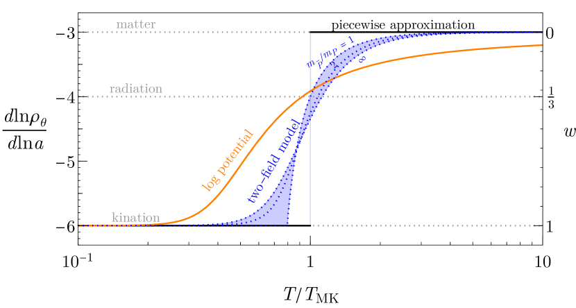
Figure 1: Scaling evolution of the energy density $\rho$ with scale factor $a$ (left axis) as well as the equation of state $w$ (right axis) as a function of temperature in units of $T_{\rm MK}$, the transition temperature from matter to kination. The colored curves are for the two-field model (blue) and the logarithmic potential (orange), whereas the step function (black) is the piecewise approximation we employ in the remainder of the paper. For the two-field model, we show the blue dotted curves for different ratios of the soft masses of the two fields $\bar{P}$ and $P$, and the blue shading indicates the entire possible range of the model.

A unique feature of our kination scenario is that matter domination preceding kination domination ends without creating entropy. This is quite different from usual matter domination, where matter domination ends by dissipation of matter into radiation creating a huge amount of entropy. Because of the absence of entropy production in our scenario, matter and kination domination can occur even after BBN and before recombination.

The precise evolution of the universe differs from the piecewise approximation and depends on the saxion potential. The evolution for the one-field model of Eq. (2.4) is derived in Co and Harigaya (2020) and reviewed in Appendix A, and is shown by the orange solid line in Fig. 1. Beyond the piecewise approximation, there is no sharply defined $T_{\rm MK}$, so we first define $T_{\rm RM}$ and $T_{\rm KR}$ by the equality of the axion energy density with the radiation energy density and then define $T_{\rm MK}\equiv T_{\rm RM}^{1/3}T_{\rm KR}^{2/3}$. The transition from matter to kination domination is not sharp, but still occurs within a temperature change of $\mathcal{O}(10)$. The evolution for the two-field model of Eq. (2.5) is derived in Appendix A and is shown by the blue-dashed lines. The evolution depends on the ratio $m_{P}/m_{\bar{P}}$, but the transition is sharper than the one-field model and occurs within a temperature change of $\mathcal{O}(1)$. As we will see, this difference shows up in the spectrum of primordial gravitational waves and allows the determination of the saxion potential.

2.3 Thermalization

As discussed in the previous subsection, the motion of the field $P$ is initiated in both angular and radial components, and the energy density associated with the radial mode is comparable to or more than the rotational energy. Since the radial mode also evolves as matter, if it is thermalized after $S$ reaches $f_{a}$, no kination-dominated era is present. Thus earlier thermalization is required. In the simplest case, we consider a Yukawa coupling between the saxion and fermions $\psi$ and $\bar{\psi}$ that couple with the thermal bath,

$$\mathcal{L}\supset y_{\psi}S\psi\bar{\psi}.$$ (2.12)

The simplest possibility is a Standard Model gauge charged fermion, but we may also consider a dark sector fermion. The thermalization rate is given by Mukaida and Nakayama (2013),

$$\Gamma_{S\psi\bar{\psi}}=by_{\psi}^{2}T,$$ (2.13)

where $b$ is a constant and is $\mathcal{O}(0.1)$ when the coupling of the fermion with the thermal bath is $\mathcal{O}(1)$. The fermion is heavy in the early universe because of a large saxion field value, $m_{\psi}=y_{\psi}S$, while the fermions themselves need to be populated in the thermal bath in order to thermalize the saxion at the temperature $T_{\rm th}$. Such a requirement, $y_{\psi}S_{\rm th}\leq T_{\rm th}$, leads to an upper bound on the Yukawa coupling as well as on the rate

$$\Gamma_{S\psi\bar{\psi}}\leq\frac{bT_{\rm th}^{3}}{S_{\rm th}^{2}}.$$ (2.14)

We obtain the same bound for a saxion-scalar coupling. For gauge boson couplings, which arise after integrating out charged fermions or scalars, the thermalization rate $\simeq 10^{-5}T^{3}/S^{2}$ Mukaida and Nakayama (2013), so the constraints on the parameter space for this case can be obtained by putting $b=10^{-5}$ in the following equations.

For a fixed $Y_{\theta}=m_{S}S_{\rm th}^{2}/(2\pi^{2}g_{*}T_{\rm th}^{3}/45)$, one can now use Eq. (2.14) to derive the maximal thermalization temperature as well as the saxion field value at the time,

$$T_{\rm th}^{\rm max} \simeq 4\times 10^{7}\ {\rm GeV}\left(\frac{b}{0.1}\right)^{\scalebox{1.01}{$\frac{1}{2}$}}\left(\frac{m_{S}}{\rm TeV}\right)^{\scalebox{1.01}{$\frac{1}{2}$}}\left(\frac{10^{3}}{Y_{\theta}}\right)^{\scalebox{1.01}{$\frac{1}{2}$}}\left(\frac{g_{*,{\rm SM}}}{g_{*}(T_{\rm th})}\right)^{\frac{3}{4}}$$ (2.15)

$$\simeq 3\times 10^{7}\ {\rm GeV}\left(\frac{b}{0.1}\right)^{\scalebox{1.01}{$\frac{1}{2}$}}\left(\frac{m_{S}}{\rm TeV}\right)^{\scalebox{1.01}{$\frac{1}{2}$}}\left(\frac{T_{\rm KR}}{10^{5}\ {\rm GeV}}\right)^{\scalebox{1.01}{$\frac{1}{2}$}}\left(\frac{10^{9}\ {\rm GeV}}{f_{a}}\right)^{\scalebox{1.01}{$\frac{1}{2}$}}\left(\frac{g_{*,{\rm SM}}}{g_{*}(T_{\rm th})}\right)^{\frac{3}{4}}\left(\frac{g_{*}(T_{\rm KR})}{g_{*,{\rm SM}}}\right)^{\frac{1}{4}},$$

$$S_{\rm th}^{\rm max} \simeq 2\times 10^{12}\ {\rm GeV}\left(\frac{b}{0.1}\right)^{\scalebox{1.01}{$\frac{3}{4}$}}\left(\frac{m_{S}}{\rm TeV}\right)^{\scalebox{1.01}{$\frac{1}{4}$}}\left(\frac{10^{3}}{Y_{\theta}}\right)^{\scalebox{1.01}{$\frac{1}{4}$}}\left(\frac{g_{*,{\rm SM}}}{g_{*}(T_{\rm th})}\right)^{\frac{5}{8}}$$ (2.16)

$$\simeq 1\times 10^{12}\ {\rm GeV}\left(\frac{b}{0.1}\right)^{\scalebox{1.01}{$\frac{3}{4}$}}\left(\frac{m_{S}}{\rm TeV}\right)^{\scalebox{1.01}{$\frac{1}{4}$}}\left(\frac{T_{\rm KR}}{10^{5}\ {\rm GeV}}\right)^{\scalebox{1.01}{$\frac{1}{4}$}}\left(\frac{10^{9}\ {\rm GeV}}{f_{a}}\right)^{\scalebox{1.01}{$\frac{1}{4}$}}\left(\frac{g_{*,{\rm SM}}}{g_{*}(T_{\rm th})}\right)^{\frac{5}{8}}\left(\frac{g_{*}(T_{\rm KR})}{g_{*,{\rm SM}}}\right)^{\frac{1}{8}}.$$

Here $Y_{\theta}$ is determined from a fixed $T_{\rm KR}$ using Eq. (2.10). In this case, the thermalization constraints can be imposed by the consistency conditions: 1) the saxion field value at thermalization must be larger than $f_{a}$, i.e., $S_{\rm th}^{\rm max}\geq f_{a}$; otherwise, thermalization would not occur or the Universe would not be kination-dominated, 2) the radiation energy density after thermalization is at least that of the saxion, i.e., $\pi^{2}g_{*}(T_{\rm th})T_{\rm th}^{4}/30\geq m_{S}^{2}(S_{\rm th}^{\rm max})^{2}$, where the inequality is saturated when the saxion dominates and reheats the universe. In fact, upon assuming the existence of kination domination, $T_{\rm RM}>T_{\rm KR}$, condition (2) automatically guarantees that (1) is satisfied. Therefore, only condition (2) is relevant and leads to the constraint on the saxion mass

$$m_{S} \lesssim 1.5\times 10^{5}\ {\rm GeV}\left(\frac{b}{0.1}\right)\left(\frac{10^{9}\ {\rm GeV}}{f_{a}}\right)^{3}\left(\frac{T_{\rm KR}}{10^{5}\ {\rm GeV}}\right)^{3}\left(\frac{g_{*}(T_{\rm KR})}{g_{*}(T_{\rm th})}\right)^{\frac{3}{2}}.$$ (2.17)

This thermalization constraint is shown as the green regions in the figures we will show in the following sections. For consistency with the assumption of the rotation in the vacuum potential, the thermal mass of $m_{S}$ must be subdominant to the vacuum one, $y_{\psi}T_{\rm th}<m_{S}$. However, using condition (2), one finds that this constraint becomes $y_{\psi}<(\pi^{2}g_{*}(T_{\rm th})/30)^{1/2}T_{\rm th}/S_{\rm th}$, which is always weaker than the earlier constraint from requiring $\psi$ in thermal equilibrium, $y_{\psi}<T_{\rm th}/S_{\rm th}$.

When the thermalization temperature is much lower than the QCD scale, additional constraints may become important Co et al. (2021b). For example, the energy density deposited into the bath (or dark radiation) at late thermalization may contribute to excessive $\Delta N_{\rm eff}$ since this energy deposit cannot be absorbed by the Standard Model bath nor diluted by the change of $g_{*}$ in the Standard Model across the QCD phase transition. Effectively, the constraint from condition (2) above is strengthened by replacing $g_{*}(T_{\rm th})$ by $7\Delta N_{\rm eff}/4$. We impose the limit $\Delta N_{\rm eff}>0.17$ from the CMB and BBN Fields et al. (2020).

In the case when $T_{\rm RM}\ll\mathcal{O}({\rm GeV})$, the saxion has to be very light and is thus subject to quantum corrections, which require the coupling $y_{\psi}<4\pi m_{S}/m_{\rm soft}$ where $m_{\rm soft}$ is the soft mass of $\psi$’s scalar partner, $\tilde{\psi}$. We do not impose this constraint since one can simply assume that $m_{\rm soft}$ is generated in the same way as and is of the same order of $m_{S}$, in which case the constraint is trivially satisfied.

One may expect additional constraints from the relic density and warmness of $\psi$ especially when $f_{a}$ is very small and $\psi$ may be very light. However, one may consider a model where $\psi$ has a sufficiently large vector-like mass and freezes out non-relativistically much before BBN (see Ref. Co et al. (2021b) for details), or $\psi$ is dark gauge-charged and effectively annihilates into massless dark gauge bosons.

3 Cosmological constraints

The axion rotations lead to matter and kination-dominated eras. If these happen close to BBN or recombination, the modified expansion rate alters primordial light element abundances or the spectrum of the CMB. Constraints from BBN divide kination into two paradigms - “early kination” for $T_{\rm KR}>\mathcal{O}({\rm MeV})$ and “late kination” with $T_{\rm RM}<\mathcal{O}(10\ {\rm keV})$. In this section, we discuss the constraints on the axion rotation on both early and late kination from BBN and the late kination from CMB.

3.1 BBN

When kination domination occurs before BBN, the strongest constraint comes from the helium abundance, since it is sensitive to the freeze-out of neutron-proton conversions, which occurs at an early stage of BBN. Using AlterBBN Arbey (2012); Arbey et al. (2020), we show the prediction on the primordial helium abundance as a function of $T_{\rm KR}$ with varying the baryon abundance within values allowed by Planck 2018 (TT,TE,EE+lowE) Aghanim et al. (2020a), together with the constraint on the abundance Zyla et al. (2020), in the left panel of Fig. 2. The width of the prediction originates from the uncertainty in nuclear reaction rates and the neutron lifetime. From this, we obtain the constraint $T_{\rm KR}\gtrsim 2.5\ {\rm MeV}$.

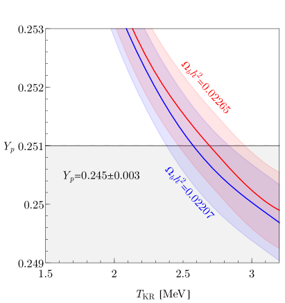
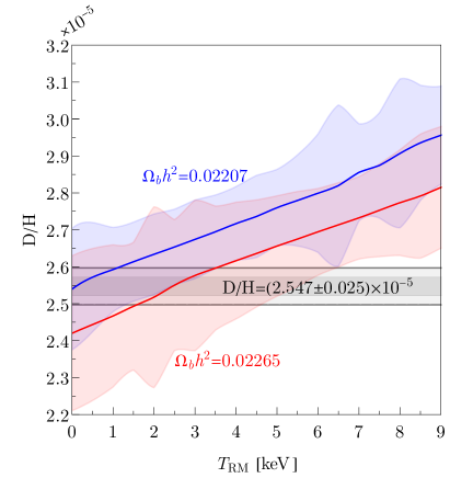
Figure 2: Primordial helium (left panel) and deuterium (right panel) abundances as a function of $T_{\rm KR}$ and $T_{\rm RM}$, respectively. The gray bands show the experimental constraints.

Here we use Planck’s allowed range for the baryon abundance with the BBN consistency condition imposed on the helium abundance for the following reason: the BBN prediction for the helium abundance with kination does not deviate from the standard prediction as much to make the helium abundance a free parameter (see Fig. 40 of Aghanim et al. (2020a)). Since BBN and CMB results for baryon abundance are in excellent agreement, relaxing the consistency condition and allowing the baryon abundance to range more freely gives very similar results for the allowed parameter space.

When kination domination occurs after BBN, but before recombination, the strongest constraint comes from the abundance of deuterium whose destruction freezes out at a late stage of BBN. We show the prediction on the primordial deuterium abundance as a function of $T_{\rm RM}$ in the right panel of Fig. 2 from which we obtain $T_{\rm RM}\lesssim 6\ {\rm keV}$.

3.2 CMB

The case of an early kination-dominated era with $T_{\rm KR}>2.5\ {\rm MeV}$ has no observable impact on the CMB. On the other hand, in the case with $T_{\rm RM}<6\ {\rm keV}$ the modified expansion rate of the universe can potentially lead to significant deviations in the evolution of modes on scales probed by the CMB.

The angular size of the sound horizon at the surface of last scattering, which is precisely measured, is one quantity that can be altered by a modified cosmic expansion history. We will develop some intuition for how the sound horizon is changed by assuming a kination-dominated era with $T_{\rm RM}<6\ {\rm keV}$ and $T_{\rm KR}>T_{eq}$, where $T_{eq}\simeq 0.8\ {\rm eV}$ is the approximate temperature at matter-radiation equality.

The comoving sound horizon can be written as

$$r_{s}(\eta)=\int^{\eta}_{0}d\eta^{{}^{\prime}}c_{s}(\eta^{{}^{\prime}}),$$ (3.1)

where $\eta$ is the comoving horizon and $c_{s}=\sqrt{\frac{1}{3\left(1+\left(\frac{3\rho_{b}}{4\rho_{\gamma}}\right)\right)}}$. Here for simplicity we will assume $c_{s}=\sqrt{\frac{1}{3}}$. We can then rewrite the integral for the comoving sound horizon at matter-radiation equality as

$$r_{s}(\eta_{eq})=\frac{\eta_{eq}}{\sqrt{3}}=\frac{1}{\sqrt{3}}\int_{0}^{a_{eq}}da\frac{1}{a^{2}H(a)},$$ (3.2)

where $a_{eq}$ is the scale factor at matter-radiation equality. The $\rm{\Lambda CDM}$ comoving sound horizon at matter-radiation equality can then be written as

$$r_{s}(\eta_{eq},\mathrm{\Lambda CDM})=\frac{1}{\sqrt{3}}\int_{a_{i}}^{a_{eq}}da\frac{1}{a^{2}_{i}H_{i}\left(\frac{a_{i}}{a}\right)^{2}}\simeq\frac{1}{\sqrt{3}}\frac{a_{eq}}{a^{2}_{i}H_{i}},$$ (3.3)

where $a_{i}\rightarrow 0$ and $H_{i}$ denote the scale factor and the Hubble scale deep in radiation domination and in the last equality we have used $a_{i}\ll a_{eq}$. For the comoving sound horizon in the case of kination cosmology, we can divide the universe into two successive eras, $a<a_{\rm MK}$ and $a_{\rm MK}\leq a\leq a_{eq}$, where we assume that $a_{eq}\gg a_{\rm KR}\gg a_{\rm RM}$. We consider the energy density of a scalar field that behaves like matter for $a<a_{\rm MK}$ and kination for $a>a_{\rm MK}$ in addition to the standard radiation density. The sound horizon in our kination cosmology up to matter-radiation equality can then be written as

$$r_{s}(\eta_{eq},{\rm kination}) =\frac{1}{\sqrt{3}}\int_{a_{i}}^{a_{\rm MK}}da\frac{1}{a^{2}H_{\rm RM}\left(\left(\frac{a_{\rm RM}}{a}\right)^{3}+\left(\frac{a_{\rm RM}}{a}\right)^{4}\right)^{1/2}}$$

$$+\frac{1}{\sqrt{3}}\int_{a_{\rm MK}}^{a_{eq}}da\frac{1}{a^{2}H_{\rm RM}\left(\left(\frac{a_{\rm RM}}{a_{\rm MK}}\right)^{3}\left(\frac{a_{\rm MK}}{a}\right)^{6}+\left(\frac{a_{\rm RM}}{a_{\rm MK}}\right)^{4}\left(\frac{a_{\rm MK}}{a}\right)^{4}\right)^{1/2}}$$

$$\simeq\frac{1}{\sqrt{3}}\frac{a_{eq}\left(1-\frac{a_{\rm KR}}{a_{eq}}\left(1+\mathcal{O}\left(\frac{a^{2/3}_{\rm RM}}{a^{2/3}_{\rm KR}},\frac{a_{\rm KR}}{a_{eq}}\right)\right)\right)}{a^{2}_{\rm RM}H_{\rm RM}},$$ (3.4)

where in the last approximation we have used $a_{i}\ll a_{eq}$ and the identity $a_{\rm RM}=\frac{a^{3}_{\rm MK}}{a^{2}_{\rm KR}}$. Here $\sqrt{2}H_{\rm RM}$ is the Hubble at the early matter radiation equality. Assuming $a_{eq}\gg a_{\rm KR}$ and $a^{2}_{i}H_{i}=a^{2}_{\rm RM}H_{\rm RM}$ in Eq. (3.3), the relative difference between the sound horizons in $\Lambda\rm{CDM}$ and kination cosmology at last scattering is approximated by

$$\frac{\Delta r_{s}(\eta_{ls})}{r_{s}(\eta_{ls},\Lambda\rm{CDM})}\simeq\frac{a_{\rm KR}}{2.4a_{eq}}=3\times 10^{-3}\left(\frac{100\ {\rm eV}}{T_{\rm KR}}\right),$$ (3.5)

where $\eta_{ls}$ is the comoving horizon at the surface of last scattering and we have assumed $a_{ls}\simeq 3a_{eq}$, $T_{eq}=0.8\ {\rm eV}$ in the last equality. Thus for large enough $T_{\rm KR}$, the deviation in the angular scale of the sound horizon at last scattering can be minimal.

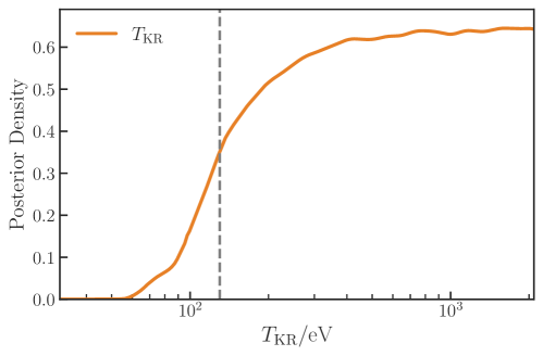
Figure 3: Posterior distribution for $T_{\rm KR}$ for a late era of kination. We use Planck temperature and polarization data (highTTTEEE+lowEE+lowTT) to constrain $T_{\rm{KR}}>130\,\rm{eV}$ at 95% (vertical dashed line). See Fig. 16 for the complete 2-dimensional posterior distributions for $\Lambda\mathrm{CDM}+T_{\mathrm{KR}}$ parameters.

The above gives some intuition for how, at fixed values of the other cosmological parameters, a kination cosmology changes the sound horizon at last scattering and by implication the angular scale of the sound horizon $\theta_{s}$. However, allowing the remaining cosmological parameters to vary—in particular $H_{0}$ or the baryon fraction $\Omega_{b}$, which enters the speed of sound—can also alter the angular scale of the sound horizon at last scattering and possibly compensate. Moreover, the enhanced Hubble rate during the early matter-dominated era, as well as kination, changes the time-temperature relationship and modifies the evolution of perturbations, which in turn substantially impacts the oscillations in the CMB power spectrum in detail. To assess the impact of low-scale kination on the CMB in full, we thus need to solve the coupled Boltzmann equations governing the evolution of gravitational and matter perturbations in the modified cosmology.

In order to quantify the bounds on the kination parameters $T_{\rm KR}$ and $T_{\rm RM}$, we modify the publicly available CMB code, CLASS Blas et al. (2011), to include kination cosmology. We also use Monte Python Brinckmann and Lesgourgues (2019), a Markov Chain Monte Carlo (MCMC) code, along with CLASS to derive the posterior probability distribution on the cosmological parameters. We assume a sudden transition between the matter-dominated and kination-dominated era at $T_{\rm MK}$. For simplicity we also fix $T_{\rm RM}=5\ {\rm keV}$, near the upper bound from BBN. We, however, find that the lower bound on $T_{\rm KR}$ from the CMB is insensitive to $T_{\rm RM}$, as the CMB is mainly probing modes that enter the horizon at lower temperatures. We consider the following cosmological parameters $\left(\Omega_{b},\,\Omega_{c},\,\Omega_{\Lambda},\,Y_{He},\,\theta_{s},\,A_{s},\,n_{s},\,\tau,\,T_{\rm KR}\right)$. We use the Planck 2018 CMB data (TT,TE,EE+lowE) to derive our constraints. The posterior distribution of $T_{\rm KR}$ is shown in Fig. 3, from which we obtain the constraint $T_{\rm KR}>130\,\rm{eV}$ at 95%. The posterior distributions of other parameters are shown in Figs. 16 and 17 in Appendix B.

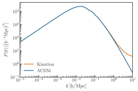
Figure 4: The linear matter power spectrum for $\Lambda$CDM and kination cosmology at $z=0$. For kination cosmology we use $T_{\rm{KR}}=130\,\rm{\ {\rm eV}}$ and $T_{\rm{RM}}=5\,\rm{\ {\rm keV}}$. Kination leads to an enhanced linear power spectrum above $k\approx\mathcal{O}(1)\,\rm{h/Mpc}$.

During early matter domination and kination (i.e., between $T_{\rm RM}$ and $T_{\rm KR}$), matter perturbations grow linearly Redmond et al. (2018). This rapid growth can result in an enhancement of the matter power spectrum on scales that were inside the horizon during the epochs of modified expansion. The excellent constraints provided by the CMB require that substantial modifications to the matter power spectrum must occur on scales $k\gg\mathcal{O}(0.1)\,\mathrm{h}\,\mathrm{Mpc^{-1}}$ (see Fig. 4). Probes of the matter power spectrum at low redshifts (such as Lyman-$\alpha$) can be used to constrain the non-linear power spectrum at $k\simeq\mathcal{O}(10)\mathrm{h}\,\mathrm{Mpc^{-1}}$ and hence raise the lower bound on $T_{\rm KR}$. However, in order to accurately derive the constraint one needs to evolve the kination matter power spectrum into the non-linear regime and then use hydrodynamical simulations to derive the Lyman-$\alpha$ flux power spectrum to compare to experiments. This is beyond the scope of the present publication, but we will return to this in future work.

4 Dark matter and baryogenesis from axion rotations

In this section, we discuss the production of axion dark matter and baryon asymmetry from axion rotations by the kinetic misalignment and axiogenesis mechanisms in the following subsections, respectively. We show the implications of these mechanisms for the parameter space $(f_{a},m_{S},Y_{\theta},m_{a})$.

4.1 Axion dark matter from kinetic misalignment

Axion rotations can lead to a larger axion abundance today via the kinetic misalignment mechanism Co et al. (2020a) than that from the conventional misalignment mechanism Preskill et al. (1983); Abbott and Sikivie (1983); Dine and Fischler (1983). As long as the axion field velocity is much larger than its mass $\dot{\theta}\gg m_{a}$, the axion continues to run over the potential barriers. If this motion continues past the time when the mass is equal to Hubble, then the axion kinetic energy $\dot{\theta}^{2}f_{a}^{2}$ is much larger than the maximum possible potential energy $\theta_{i}^{2}m_{a}^{2}f_{a}^{2}$ in the conventional case and thus the abundance is enhanced.

Even when the axion field velocity is larger than the mass, the axion self-interactions can cause parametric resonance (PR) Dolgov and Kirilova (1990); Traschen and Brandenberger (1990); Kofman et al. (1994); Shtanov et al. (1995); Kofman et al. (1997), which fragments the axion rotation into axion fluctuations Jaeckel et al. (2017); Berges et al. (2019); Fonseca et al. (2020). The production of fluctuations by PR occurs at an effective rate given by Fonseca et al. (2020)

$$\Gamma_{\rm PR}=\frac{m_{a}^{4}}{\dot{\theta}^{3}}.$$ (4.1)

On the other hand, the axion momentum $k_{\rm PR}$ generated at the time of PR is of order $\dot{\theta}/2$ due to the resonance condition. Therefore, the abundance of the axion is estimated as

$$\frac{\rho_{a}}{s}=m_{a}Y_{a}=Cm_{a}\frac{\rho_{\theta}/s}{k_{\rm PR}}=Cm_{a}Y_{\theta},$$ (4.2)

where the axion yield $Y_{a}$ is approximately conserved after PR. Here $C$ is a factor that should be determined by numerical computation. In Ref. Co et al. (2020a), $C\simeq 2$ was derived assuming the coherence of the axion rotation throughout the evolution. As noted in Ref. Co et al. (2021b), the axion abundance is reduced by an $\mathcal{O}(1)$ factor in comparison with the estimation in Ref. Co et al. (2020a) because of the extra energy of axions from non-zero momenta sourced by PR. Just after PR effectively occurs, the number-changing scattering rate of axion fluctuations is comparable to the Hubble expansion rate while axion fluctuations are over-occupied, so the number density may be further reduced by an $\mathcal{O}(1)$ factor, which should be determined by lattice computation; see also the discussion in Micha and Tkachev (2003, 2004); Co et al. (2018). We use the reference value $C=1$ in this paper and demonstrate the impact of $C<1$ on observations by showing results for $C=0.3$. Requiring axion dark matter from the kinetic misalignment mechanism, we obtain a prediction on $T_{\rm KR}$,

$$T_{\rm KR} \simeq 2.4\times 10^{6}\ {\rm GeV}\times C\left(\frac{f_{a}}{10^{9}\ {\rm GeV}}\right)\left(\frac{m_{a}}{6~{}{\rm meV}}\right)\left(\frac{g_{*,{\rm SM}}}{g_{*}(T_{\rm KR})}\right)^{\scalebox{1.01}{$\frac{1}{2}$}}$$ for ALPs

$$\simeq 2.4\times 10^{6}\ {\rm GeV}\times C\left(\frac{g_{*,{\rm SM}}}{g_{*}(T_{\rm KR})}\right)^{\scalebox{1.01}{$\frac{1}{2}$}} \text{for the QCD axion}.$$ (4.3)

The prediction for an ALP is shown by the purple dashed lines in the left panel of Fig. 5. To avoid overproduction of axion dark matter by the kinetic misalignment mechanism, this prediction is also a lower bound on $T_{\rm KR}$. The bound can be avoided if the rotation is washed out at $T<T_{\rm KR}$. This is difficult for the QCD axion with the Standard Model because of the suppression of the wash-out rate by the small up Yukawa coupling Co and Harigaya (2020); McLerran et al. (1991), but is possible in extensions of the Standard Model. We do not pursue this possibility further. The prediction on $m_{a}$ as a function on $f_{a}$ and $T_{\rm KR}$ is shown in the right panel of Fig. 5; here the prediction is also an upper bound on $m_{a}$.

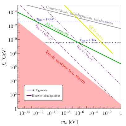
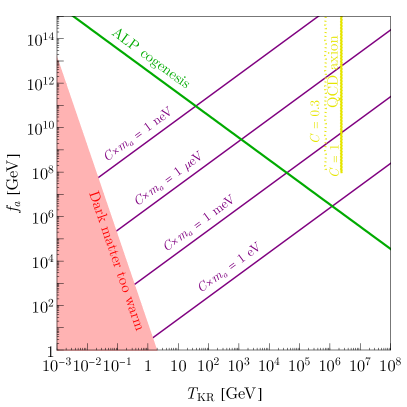
Figure 5: Axion dark matter and the baryon asymmetry from axion rotation. Left panel: in the axion parameter space, contours of $T_{\rm KR}=1\ {\rm GeV}$ ($1\ {\rm TeV}$) are shown in dashed (dot-dashed) lines as predicted by dark matter from kinetic misalignment (purple) and for the baryon asymmetry from minimal ALPgenesis (blue). The contours intersect along the green line where dark matter and the baryon asymmetry are simultaneously explained as in ALP cogenesis. Right panel: the purple lines are the contours of the mass of axion dark matter predicted by kinetic misalignment as a function of $f_{a}$ and $T_{\rm KR}$. In both panels, the red region is excluded by the warmness of axion dark matter from kinetic misalignment. The yellow line in either plot shows the prediction assuming a QCD axion which terminates at $f_{a}=10^{8}\ {\rm GeV}$ since lower $f_{a}$ is disfavored by astrophysical constraints.

Parametric resonance becomes effective when $\Gamma_{\rm PR}\simeq H$. One can obtain $\dot{\theta}(T)$, which is relevant for $\Gamma_{\rm PR}$, by using Eq. (2.3) and requiring the axion abundance in Eq. (4.2) to reproduce the observed dark matter abundance $\rho_{\rm DM}/s\simeq 0.44$ eV. The temperature $T_{\rm PR}$ when PR occurs is given by

$$T_{\rm PR}\simeq 100\ {\rm MeV}\left(\frac{f_{a}}{10^{9}\ {\rm GeV}}\right)^{\scalebox{1.01}{$\frac{6}{11}$}}\left(\frac{m_{a}}{10^{-6}\ {\rm eV}}\right)^{\scalebox{1.01}{$\frac{7}{11}$}}\left(\frac{g_{*,{\rm SM}}}{g_{*}(T_{\rm PR})}\right)^{\scalebox{1.01}{$\frac{7}{22}$}}C^{3/11},$$ (4.4)

where we assume that the axion mass at $T=T_{\rm PR}$, is the same as the one in vacuum, $m_{a}(T_{\rm PR})=m_{a}$, and the saxion is at the minimum of the potential, $S(T_{\rm PR})=f_{a}$. As with PR production from radial motion of the symmetry breaking field Co et al. (2018, 2020b), the produced axions are initially relativistic. They may become cold enough to be dark matter by red-shifting, and will have residual warmness Berges et al. (2019); Co et al. (2021b). They become non-relativistic at temperature

$$T_{\rm NR}\simeq 10\ {\rm MeV}\left(\frac{f_{a}}{10^{9}\ {\rm GeV}}\right)^{\scalebox{1.01}{$\frac{10}{11}$}}\left(\frac{m_{a}}{10^{-6}\ {\rm eV}}\right)^{\scalebox{1.01}{$\frac{8}{11}$}}\left(\frac{g_{*,{\rm SM}}}{g_{*}(T_{\rm PR})}\right)^{\frac{1}{33}}C^{5/11}.$$ (4.5)

For sufficiently small $m_{a}$ and/or $f_{a}$, these axions are too warm to be dark matter based on the current warmness constraint from the Lyman-$\alpha$ measurements Iršič et al. (2017), $T_{\rm NR}>5\ {\rm keV}$. This constraint is shown by the red regions of Fig. 5.

4.2 Baryon asymmetry from axiogenesis

The observed cosmological excess of matter over antimatter can also originate from the axion rotation. The $U(1)$ charge associated with the rotation defined in Eq. (2.3) can be transferred to the baryon asymmetry as shown in Co and Harigaya (2020); Co et al. (2021c, a). In the case of the QCD axion, the strong anomaly necessarily transfers the rotation into the quark chiral asymmetry, which is distributed into other particle-antiparticle asymmetry. More generically, the couplings of the QCD axion or an ALP with the thermal bath can transfer the rotation into particle-antiparticle asymmetry. The particle-antiparticle asymmetry can be further transferred to baryon asymmetry via processes that violate the baryon number. We call this scheme, applicable to the QCD axion and ALPs, axiogenesis. To specifically refer to the QCD axion and ALPs, we use QCD axiogenesis and ALPgenesis, respectively.

4.2.1 Minimal axiogenesis

In the minimal scenario, which we call minimal axiogenesis, the particle-antiparticle asymmetry is reprocessed into the baryon asymmetry via the electroweak sphaleron processes. If the QCD axion or an ALP has an electroweak anomaly, then the rotation can directly produce the baryon asymmetry by the electroweak sphaleron processes. The contribution to the yield of the baryon asymmetry is given by Co and Harigaya (2020)

$$Y_{B}=\frac{n_{B}}{s}=\left.\frac{45c_{B}}{2g_{*}\pi^{2}}\frac{\dot{\theta}}{T}\right|_{T=T_{\rm ws}}\simeq 8.2\times 10^{-11}\left(\frac{c_{B}}{0.1}\right)\left(\frac{\dot{\theta}(T_{\rm ws})}{5\ {\rm keV}}\right)\left(\frac{130\ {\rm GeV}}{T_{\rm ws}}\right),$$ (4.6)

where $T_{\rm ws}$ is the temperature at which the electroweak sphaleron processes go out of equilibrium and is approximately $130\ {\rm GeV}$ in the Standard Model D’Onofrio et al. (2014), and $c_{B}$ is a model-dependent coefficient given in Ref. Co et al. (2021c) that parameterizes the anomaly coefficients and the axion-fermion couplings. When the transfer is dominated by axion-gauge boson couplings, $c_{B}$ is typically $\mathcal{O}(0.1)$, while if dominated by axion-fermion couplings, it can be much smaller.

For the QCD axion, to produce sufficient $Y_{B}$ and to avoid overproduction of dark matter by kinetic misalignment requires that $f_{a}\lesssim 10^{7}\ {\rm GeV}c_{B}/C$, which is disfavored by astrophysical constraints Ellis and Olive (1987); Raffelt and Seckel (1988); Turner (1988); Mayle et al. (1988); Raffelt (2008); Payez et al. (2015); Bar et al. (2020) unless $c_{B}/C>10$. The baryon asymmetry can be enhanced if the electroweak phase transition occurs at a higher temperature,

$$T_{\rm ws}\geq 1~{}{\rm TeV}\left(\frac{f_{a}}{10^{8}\ {\rm GeV}}\right)^{\scalebox{1.01}{$\frac{1}{2}$}}\left(\frac{0.1}{c_{B}}\right)C^{1/2},$$ (4.7)

with both dark matter and baryon asymmetry of the universe explained by the rotation of the QCD axion when the inequality is saturated.

For an ALP, we may choose sufficiently small $m_{a}$ to avoid the over production without modifying the electroweak phase transition temperature. Requiring that the baryon yield of Eq. (4.6) match the observed baryon asymmetry gives a constraint on $\dot{\theta}(T_{ws})$; using Eq. (2.10) this can be converted to a prediction for $T_{\rm KR}$

$$T_{\rm KR}=3.5~{}{\rm TeV}\left(\frac{10^{9}\ {\rm GeV}}{f_{a}}\right)\left(\frac{f_{a}}{S(T_{\rm ws})}\right)^{2}\frac{c_{B}}{0.1}\left(\frac{g_{*,{\rm SM}}}{g_{*}}\right)^{\scalebox{1.01}{$\frac{1}{2}$}},$$ (4.8)

which is shown by the blue dot-dashed line in the left panel of Fig. 5, assuming $S(T_{\rm ws})=f_{a}$. Note that this is necessarily the case when $T_{\rm MK}>T_{\rm ws}$. For lower $T_{\rm MK}$, $S(T_{\rm ws})>f_{a}$ is possible. Since $\dot{\theta}\simeq m_{S}$ when $S>f_{a}$ and $\dot{\theta}\propto T^{3}$ after $S=f_{a}$, we have $\dot{\theta}(T_{\rm ws})\lesssim m_{S}$ and therefore the saxion mass is predicted to be

$$m_{S}>5\ {\rm keV}\left(\frac{0.1}{c_{B}}\right).$$ (4.9)

The bound is saturated when $S(T_{\rm ws})>f_{a}$, which is the case if $T_{\rm MK}<T_{\rm ws}$.

Both dark matter and baryon asymmetry of the universe is explained by the axion rotation, which is called ALP cogenesis Co et al. (2021c), when

$$m_{a}=8.5~{}{\rm\mu eV}\left(\frac{10^{9}\ {\rm GeV}}{f_{a}}\right)^{2}\left(\frac{f_{a}}{S(T_{\rm ws})}\right)^{2}\left(\frac{c_{B}}{0.1}\right)\left(\frac{1}{C}\right).$$ (4.10)

This prediction is shown by the green lines in Fig. 5.

4.2.2 $B-L$ number violation by new physics

In the presence of an operator that violates lepton number and generates Majorana neutrino masses, the transfer of asymmetries can be more efficient. The operator creates a non-zero $B-L$ number, which is preserved by Standard Model electroweak sphaleron processes. Since the production of $B-L$ at high temperatures depends on whether the lepton number violating interactions are in equilibrium, the determination of the final baryon number in this scenario is sensitive to the full cosmological evolution. As an example, for the models studied in Ref. Co et al. (2021a), the baryon asymmetry is given by

$$Y_{B}\simeq 8.7\times 10^{-11}N_{\rm DW}\left(\frac{c_{B}}{0.1}\right)\left(\frac{g_{\rm MSSM}}{g_{*}}\right)^{\scalebox{1.01}{$\frac{3}{2}$}}\left(\frac{\bar{m}^{2}}{0.03~{}{\rm eV}^{2}}\right)\left(\frac{m_{S}}{30\ {\rm TeV}}\right)\left(\frac{D}{23}\right),$$ (4.11)

where $\bar{m}^{2}=\Sigma_{i}m^{2}_{i}$ is the sum of the square of the neutrino masses $m_{i}$, $N_{\rm DW}$ is the domain wall number (which is assumed to be unity in other parts of the paper), and the function $D$ parameterizes the different cosmological scenarios. In particular, $D=\mathcal{O}(20)$ for the case where no entropy is produced after the production of $B-L$ and is logarithmically dependent on $f_{a}$ as well as the saxion field values at various temperatures. Alternatively, if the saxion dominates before decaying and reheating the Universe $D=1$, and (4.11) yields a sharp prediction for $m_{S}$, valid when the saxion is thermalized before settling to $f_{a}$. For details of the evaluation of $D$, one can refer to Ref. Co et al. (2021a). Regardless, the saxion mass is generically predicted to be $\mathcal{O}(30-10^{4})\ {\rm TeV}\times(0.1/c_{B})$ by this baryogenesis mechanism, named lepto-axiogenesis generically, QCD lepto-axiogenesis for the QCD axion, and lepto-ALPgenesis for the ALP. While $m_{S}\ll 30\ {\rm TeV}$ appears difficult based on Eq. (4.11), the case of TeV scale supersymmetry is possible in some special cases presented in Ref. Co et al. (2021a), using a thermal potential.

Other axiogenesis scenarios are are also considered in the literature Harigaya and Wang (2021); Chakraborty et al. (2021). Baryon asymmetry may be dominantly produced at a temperature $T_{\rm dec}$ with $Y_{B}\sim\dot{\theta}/T\times{\rm min}(1,\Gamma_{B}/H)$, where $\Gamma_{B}$ is the transfer rate of the axion rotation into baryon asymmetry. For models with $T_{\rm dec}>T_{\rm ws}$, the lower bound on $m_{S}$ is generically stronger than that for ALPgenesis.

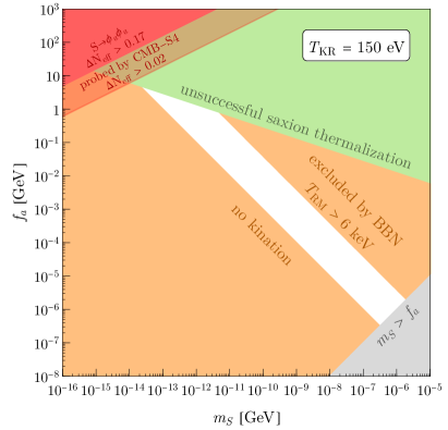
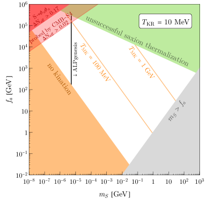
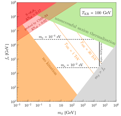
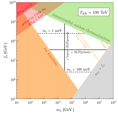
Figure 6: The unshaded regions show the allowed parameter space for axion kination for the fixed values of $T_{\rm KR}$ labeled in each panel. Contours of $T_{\rm MK}$ are shown in these regions with kination. The excluded shaded regions are discussed in the text. To achieve minimal ALPgenesis, the parameter space collapses into $m_{S}\simeq 5\ {\rm keV}(0.1/c_{B})$ as shown by the black solid line in the upper-right panel, or into $f_{a}$ given by Eq. (4.8) with $S(T_{\rm ws})=f_{a}$ as shown by the black solid line in the lower-right panel, where we take $c_{B}=0.1$. On the other hand, lepto-ALPgenesis restricts the parameter space to $m_{S}\gtrsim 30\ {\rm TeV}$. The axion cannot constitute dark matter via kinetic misalignment in the upper panels due to the warmness constraint in Eq. (4.5).

4.2.3 Implications to axion kination parameters

In Fig. 6, we show constraints on the parameter space for several reference values of $T_{\rm KR}$. The green-shaded regions are excluded because of the failure of thermalization of the initial radial oscillation, as described in Sec. 2.3. No kination-dominated era arises in the lower orange-shaded regions. The upper orange-shaded region in the upper-left panel is excluded by BBN. The orange lines are the contours of $T_{\rm MK}$. In the gray-shaded region, $m_{S}$ is above $f_{a}$ and the perturbativity of the potential of the $U(1)$ symmetry breaking field breaks down. The red-shaded region is excluded by dark radiation produced by the decay of thermalized saxions into axions. The remaining unshaded regions give the allowed parameter space where axion rotation leads to realistic cosmologies with early eras of matter and kination domination. Contours of $T_{\rm MK}$ are shown in these kination regions.

In the lower two panels, the horizontal black dashed lines show the prediction for the axion mass from requiring that the observed dark matter result from the kinetic misalignment mechanism. In the upper two panels, axion dark matter from kinetic misalignment is excluded as it is too warm.

In the upper-left panel, no parameter region is consistent with the lower bound on $m_{S}$ from axiogenesis above the electroweak scale. In the upper-right panel, $m_{S}$ can be above the keV scale. $T_{\rm MK}$ is below the electroweak scale, so $S(T_{\rm ws})>f_{a}$ and $\dot{\theta}_{\rm ws}=m_{S}=5$ keV $(0.1/c_{B})$ is required. In the lower-left panel, $T_{\rm MK}>100$ GeV, so that the condition for successful minimal ALPgenesis is given by (4.8) with $S(T_{\rm ws})=f_{a}$, requiring $c_{B}\ll 1$. Lepto-ALPgenesis is possible to the right of the black solid line. In the lower-right panel, where $T_{\rm MK}>100$ GeV, minimal ALPgenesis requires $f_{a}$ shown by the vertical black solid line according to Eq. (4.8) with $c_{B}=0.1$. Lower $f_{a}$ is possible if $c_{B}<0.1$.

5 Gravitational waves

In this section, we discuss how the spectrum of primordial gravitational waves is modified by eras of matter and kination domination generated from axion rotation, as discussed in Sec. 2. We consider gravitational waves created by quantum fluctuations during inflation and by local cosmic strings. In both production mechanisms, the spectrum is nearly flat in the standard cosmology with radiation domination. As we will see, the evolution of a universe with successive eras dominated by radiation, matter, kination, and back to radiation induces a triangular peak in the gravitational wave spectrum that can provide a unique signal for axion rotation and kination cosmology.

5.1 From inflation

We first discuss the primordial gravitational waves produced from quantum fluctuations during inflation Starobinsky (1985). In the standard cosmology with radiation domination, the spectrum is nearly flat for the following reason. After inflation, a given mode $k$ is frozen outside the horizon, $k<H$. As the mode reenters the horizon, $k>H$, it begins to oscillate and behaves as radiation. The energy density of the mode at that point $\sim k^{2}h^{2}(k)M_{\rm Pl}^{2}$, where $h$ is the metric perturbation, whose spectrum is almost flat for slow-roll inflation. Since $k\sim H$ at the beginning of the oscillation, the energy density of the gravitational waves normalized by the radiation energy density $\sim H^{2}M_{\rm Pl}^{2}$ is nearly independent of $k$ up to a correction by the degree of freedom of the thermal bath

During matter or kination domination in our scenario, the energy density at the horizon crossing is still $H^{2}h^{2}M_{\rm Pl}^{2}$, but the radiation energy density is now much smaller than $H^{2}M_{\rm Pl}^{2}$. As a result, the energy density of gravitational waves with a mode $k$ is inversely proportional to the fraction of the radiation energy density to the total energy density when the mode enters the horizon. This means that the spectrum should feature a triangular peak in axion kination. The modes that enter the horizon at $T>T_{\rm RM}$ are not affected and remain flat. (See, however, a comment below). Therefore, as the horizon-crossing temperature decreases below $T_{\rm RM}$, the gravitational waves are enhanced and reach the maximal value at $T_{\rm MK}$, where the fraction of the radiation energy is minimized. The gravitational wave strength decreases again for the horizon crossing temperatures below $T_{\rm MK}$, and returns to a flat spectrum below $T_{\rm KR}$. Note that gravitational waves that enter the horizon during matter domination are also enhanced because of the absence of entropy production after matter domination. We use an analytical approximation where each mode begins oscillations suddenly at the horizon crossing. Also approximating the evolution of $H$ by a piecewise function with kinks at the three transition, the resultant spectrum of gravitational waves is given by

$$\Omega_{\rm GW}h^{2} \simeq 1.4\times 10^{-17}\left(\frac{V_{\rm inf}^{1/4}}{10^{16}\ {\rm GeV}}\right)^{4}\left(\frac{g_{*,{\rm SM}}}{g_{*}(T_{\rm hc})}\right)^{\scalebox{1.01}{$\frac{1}{3}$}}\begin{cases}1&\text{RD~{}:~{}}f_{\rm RM}<f\\ \left(\frac{f_{\rm RM}}{f}\right)^{2}&\text{MD~{}:~{}}f_{\rm MK}<f<f_{\rm RM}\\ \frac{f}{f_{\rm KR}}&\text{KD~{}:~{}}f_{\rm KR}<f<f_{\rm MK}\\ 1&\text{RD~{}:~{}}f<f_{\rm KR}\end{cases},$$ (5.1)

$$f_{\rm RM,KR} \simeq 27~{}\mu{\rm Hz}\left(\frac{T_{\rm RM,KR}}{{\rm TeV}}\right)\left(\frac{g_{*}(T_{\rm RM,KR})}{g_{*,{\rm SM}}}\right)^{\scalebox{1.01}{$\frac{1}{6}$}},$$ (5.2)

$$f_{\rm MK} =(f_{\rm RM}^{2}f_{\rm KR})^{1/3}\simeq 27~{}\mu{\rm Hz}\left(\frac{T_{\rm RM}}{{\rm TeV}}\right)^{\scalebox{1.01}{$\frac{2}{3}$}}\left(\frac{T_{\rm KR}}{{\rm TeV}}\right)^{\scalebox{1.01}{$\frac{1}{3}$}}\left(\frac{g_{*}(T_{\rm RM})}{g_{*,{\rm SM}}}\right)^{\scalebox{1.01}{$\frac{1}{9}$}}\left(\frac{g_{*}(T_{\rm KR})}{g_{*,{\rm SM}}}\right)^{\scalebox{1.01}{$\frac{1}{18}$}},$$ (5.3)

where $V_{\rm inf}$ is the potential energy during inflation. We normalize the spectrum to match a full numerical result at $f<f_{\rm KR}$ and $f>f_{\rm RM}$, which is found to be consistent with the result of the numerical computation in Ref. Saikawa and Shirai (2018).

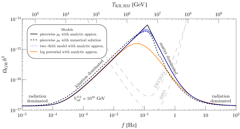
Figure 7: An illustration of the model dependence in the primordial gravitational wave spectrum. Here we fix $T_{\rm KR}=10^{4}\ {\rm GeV}$, $T_{\rm RM}=10^{8}\ {\rm GeV}$ (and accordingly $T_{\rm MK}\simeq 2\times 10^{5}\ {\rm GeV}$), and the inflationary energy scale $V_{\rm inf}^{1/4}=10^{16}\ {\rm GeV}$. The black lines are for the case where the rotation energy density $\rho_{\theta}$ follows a piecewise scaling when $T\lessgtr T_{\rm MK}$ as shown in Fig. 1. The solid (dashed) black lines are obtained from an analytic (numerical) derivation of the evolution of the metric perturbations. The colored curves are for the two-field model (blue) and the logarithmic potential (orange) with evolution demonstrated in Fig. 1. For the two-field model, we show the blue dotted curves for different ratios of the soft masses of the two fields $\bar{P}$ and $P$, $m_{\bar{P}}/m_{P}=1,2,\infty$ from top to bottom.

In Fig. 7, we illustrate the spectrum of gravitational waves in axion kination. Throughout this paper, we use the sensitivity curves derived in Ref. Schmitz (2021) for NANOGrav McLaughlin (2013); Arzoumanian et al. (2018); Aggarwal et al. (2019); Brazier et al. (2019), PPTA Manchester et al. (2013); Shannon et al. (2015), EPTA Kramer and Champion (2013); Lentati et al. (2015); Babak et al. (2016), IPTA Hobbs et al. (2010); Manchester (2013); Verbiest et al. (2016); Hazboun et al. (2018), SKA Carilli and Rawlings (2004); Janssen et al. (2015); Weltman et al. (2020), LISA Amaro-Seoane et al. (2017); Baker et al. (2019), BBO Crowder and Cornish (2005); Corbin and Cornish (2006); Harry et al. (2006), DECIGO Seto et al. (2001); Kawamura et al. (2006); Yagi and Seto (2011), CE Abbott et al. (2017); Reitze et al. (2019) and ET Punturo et al. (2010); Hild et al. (2011); Sathyaprakash et al. (2012); Maggiore et al. (2020), and aLIGO and aVirgo Harry (2010); Aasi et al. (2015); Acernese et al. (2015); Abbott et al. (2021). The black solid and dashed curves are both based on the piecewise approximation of the $\rho_{\theta}$ contribution to the Hubble rate, whereas the black solid (dashed) curve is with the analytical approximation (numerical solution) of the horizon crossing. Here $H$ is computed by the addition of $\rho_{\theta}$ and the radiation energy density, so smoothly changes around $T_{\rm RM}$ and $T_{\rm KR}$. As the analytic approximation reproduces the numerical result very well, we use the analytic approximation of the horizon crossing in the remainder of this paper. The blue dotted and orange solid lines show the spectrum for the two-field model and the log potential, respectively. The spectrum for the two-field model is close to that for the piecewise approximation, while that for the log potential deviates from them. Remarkably, the measurement of the gravitational wave spectrum around the peak can reveal the shape of the potential that spontaneously breaks the $U(1)$ symmetry.

We comment on possible further modification of the spectrum. Axion kination relies on a nearly quadratic saxion potential, which is natural in supersymmetric theories. The degrees of freedom of the thermal bath change by about a factor of two across the superpartner mass threshold, suppressing the gravitational wave signals by a few tens of a percent at high frequency Watanabe and Komatsu (2006). This depends on the superpartner masses, and we do not include this effect for simplicity. We also assume that the radial mode of $P$ does not dominate the energy density of the universe. If it does, entropy is created by the thermalization of the radial mode and gravitational waves at $f>f_{\rm RM}$ can be suppressed. If the initial rotation before thermalization is highly elliptical, after the thermalization the universe is radiation dominated for a long time because of the radial mode energy much larger than the angular mode energy, so the suppression occurs at $f\gg f_{\rm RM}$. If the initial rotation is close to a circular one, the universe is radiation dominated only for a short period, so the suppression occurs right above $f_{\rm RM}$. In principle, we can learn about the very UV dynamics of axion rotations through the observations of gravitational waves.

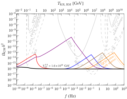
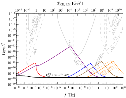
Figure 8: GW spectra from inflation for inflationary energy scale $V_{\rm inf}^{1/4}$ of $1.6\times 10^{16}$ GeV (left panel) and $6\times 10^{15}$ GeV (right panel). Each panel contains various choices of $(T_{\rm KR},T_{\rm RM})$. The left (right) vertex of each triangle approximately indicates the choice of $T_{\rm KR}$ ($T_{\rm RM}$) labeled at the top axis, while $T_{\rm MK}^{3}=T_{\rm RM}T_{\rm KR}^{2}$. The $(T_{\rm KR},T_{\rm RM})$ choices are $(3\ {\rm MeV},3\ {\rm GeV})$ for red, $(10^{-2},10^{7})\ {\rm GeV}$ for purple, $(10^{4},8\times 10^{7})\ {\rm GeV}$ for blue, and $(10^{5},3\times 10^{9})\ {\rm GeV}$ for brown. Finally, for QCD axion dark matter to be produced by kinetic misalignment with $C=1$ and $0.3$, $T_{\rm KR}$ is predicted to be $2\times 10^{6}$ and $7\times 10^{5}$ GeV as shown in the solid and dotted orange curves with the maximal $T_{\rm RM}$ of $7\times 10^{10}$ and $4\times 10^{10}$ GeV allowed by the constraints shown in Fig. 9. These curves assume $g_{*}(T)$ for the Standard Model and $H$ with individual energy density contributions including a piecewise $\rho_{\theta}$.

In Fig. 8, we show the gravitational wave spectra for two choices of the inflaton potential energy scale $V_{\rm inf}$. The inflationary energy scales of $V_{\rm inf}^{1/4}=1.6\times 10^{16}$ GeV and $6\times 10^{15}$ GeV correspond to the tensor fractions of $r=0.056$ near the upper bound from the CMB Aghanim et al. (2020a) and $r=0.001$ near the sensitivity limit of future CMB observations Abazajian et al. (2016), respectively. We show the spectrum for several sets of $(T_{\rm KR},T_{\rm RM})$ in different colored curves.

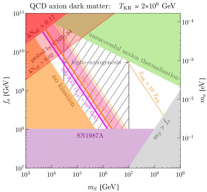
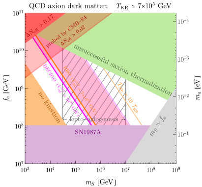
Figure 9: Parameter space for the QCD axion dark matter produced by kinetic misalignment, which predicts $T_{\rm KR}\simeq C\times 2\times 10^{6}\ {\rm GeV}$ as can be seen in Fig. 5. The left (right) panel assumes $C=1~{}(0.3)$. The regions above the thick magenta and orange lines lead to a primordial gravitation wave signal that can be probed by DECIGO and BBO for the labeled choices of $V_{\rm inf}^{1/4}$, while within the adjacent transparent shadings, the peak of the spectrum can be detected by each observatory. The signal is made possible by the kination era; otherwise, $V_{\rm inf}^{1/4}>1.2\times 10^{16}\ {\rm GeV}$ is required for DECIGO.

The spectrum shown in the solid (dotted) orange curve corresponds to the value of $T_{\rm KR}$ predicted from QCD axion dark matter via the kinetic misalignment mechanism with $C=1$ ($C=0.3$) according to Eq. (4.1), with the maximal $T_{\rm RM}$ allowed by the constraints shown in Fig. 9. In Fig. 9, we explore the parameter space for the QCD axion for $C=1$ (left panel) and $C=0.3$ (right panel). Most features of Fig. 9 are analogous to those in Fig. 6, whereas the gray hatched region indicates the range of $m_{S}$ compatible with lepto-axiogenesis based on Eq. (4.11). If the inflation scale is not much below the present upper bound, DECIGO and BBO can detect the modification of the spectrum arising from the QCD axion kination era if the parameters of the theory lie anywhere above the thick magenta and orange lines in Fig. 9. Inside the transparent shaded regions with $T_{\rm RM}$ lower than the maximum allowed, BBO and DECIGO can also observe the peak of the spectrum peculiar to axion kination and identify how the Peccei-Quinn symmetry is spontaneously broken. If $C<1$ and $T_{\rm RM}$ is close to the maximum, CE can also observe the signal, but the inflation scale must be almost at the present upper bound as seen in Fig. 8.

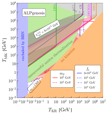
Figure 10: Possible ranges of temperatures are shown for ALPgenesis assuming $c_{B}=0.1$. Contours of required $f_{a}$ and $m_{S}$ are shown by the blue and red lines respectively. White and transparent regions are allowed. Thanks to a kination era, the primordial gravitational waves for $V_{\rm inf}^{1/4}=10^{16}\ {\rm GeV}$ (left panel) and $6\times 10^{15}\ {\rm GeV}$ (right panel) become detectable by the experiments specified next to the colored sensitivity curves. The transparent colored shading for each gravitational wave observatory indicates the regions where the peak in the gravitational wave spectrum falls within the experimental sensitivity.

The parameter space for ALPgenesis is shown in Fig. 10. In the allowed parameter region at the bottom-left of the figure, $T_{\rm MK}$ is below the electroweak scale and $\dot{\theta}_{\rm ws}\simeq m_{S}=5$ keV $(0.1/c_{B})$. $f_{a}$ is determined according to Eqs. (2.9) and (2.10). In the allowed parameter region in the upper-right corner, $T_{\rm MK}$ is above the electroweak scale and $S(T_{\rm ws})=f_{a}$, so $f_{a}$ is determined by Eq. (4.8). $m_{S}$ is determined by Eqs. (2.9) and (2.10). Above each colored line, each experiment can detect the gravitational wave spectrum enhanced by axion kination. In the transparent shaded region, the triangular peak can be detected. Here we take $c_{B}=0.1$. For smaller $c_{B}$, the prediction on $f_{a}$ and $m_{S}$ becomes larger, and the allowed range of $(T_{\rm KR},T_{\rm MK})$ expands, as can be seen from the black solid lines in Fig. 6.

The parameter space for lepto-ALPgenesis is shown in Fig. 11. Here $m_{S}$ is fixed so that the observed baryon asymmetry is explained by lepto-ALPgenesis; see Eq. (4.11). $f_{a}$ is then fixed by Eqs. (2.9) and (2.10). The meaning of shaded regions and contours are the same as in Fig. 10.

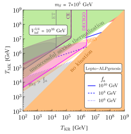
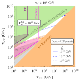
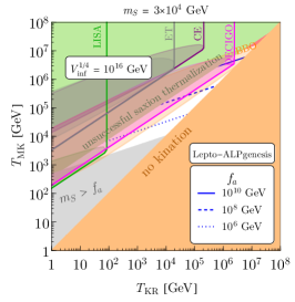
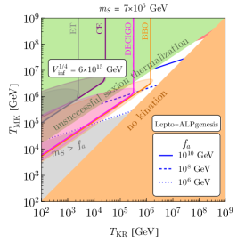
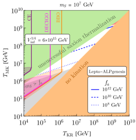
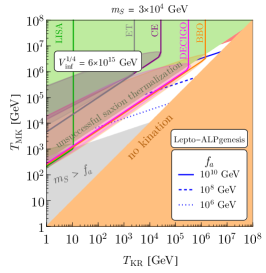
Figure 11: Possible ranges of temperatures are shown for lepto-ALPgenesis. The left two columns are for the case with entropy production from saxion domination ($D=1$), while the right column assumes radiation domination ($D=\mathcal{O}(20)$) with degenerated neutrinos. These different cases are explained in Sec. 4.2 and Ref. Co et al. (2021a). The dark matter abundance is explained by an appropriate ALP mass determined by $f_{a}$ and $T_{\rm KR}$ using Fig. 5. Thanks to a kination era, the primordial gravitational waves for $V_{\rm inf}^{1/4}=10^{16}\ {\rm GeV}$ ($6\times 10^{15}\ {\rm GeV}$) in the upper (lower) panels become detectable by the experiments labeled next to the colored sensitivity curves. The transparent colored shadings indicate that the peak of the gravitational wave spectrum due to kination lies inside the corresponding experimental reach.

5.2 From cosmic strings

We next discuss gravitational waves emitted from local cosmic strings Vachaspati and Vilenkin (1985). Local cosmic strings are topological defects produced upon gauge symmetry breaking in the early universe, such as $U(1)$ symmetry breaking Kibble (1976). The breaking of a local $U(1)$ symmetry, and hence formation of a cosmic string network, arises in many theories beyond the Standard Model. For example, one of the best motivated cases is $U(1)_{\rm B-L}$, which is the unique $U(1)$ symmetry that does not have a mixed anomaly with the Standard Model gauge symmetry. Moreover, $U(1)_{\rm B-L}$ can be embedded into $SO(10)$ together with the Standard Model gauge group, and whose spontaneous symmetry breaking can provide the right-handed neutrino masses in the see-saw mechanism Minkowski (1977); Yanagida (1979); Gell-Mann et al. (1979); Mohapatra and Senjanovic (1980).

After production, the cosmic string network follows a scaling law with approximately ${\mathcal{O}}(1)$ long strings per Hubble volume which is maintained from the balance between conformal expansion with the universe and losses from self-intercommutation. The self-intercommutation byproducts of the long string network lead to the formation of a network of string loops with a new loop forming nearly every Hubble time and with a loop size proportional to the horizon Vilenkin and Shellard (2000). These subhorizon loops oscillate and redshift like matter before decaying from the emission of gravitational waves. Because of the scaling law of the string network, the energy density fraction of the cosmic strings is nearly independent of temperature, and the spectrum of gravitational waves emitted from the local cosmic strings during radiation domination is nearly flat.

During kination or matter domination by axion rotation, the size of the horizon for a given temperature is smaller than it would be in a radiation dominated universe. This enhances the energy density of strings relative to the radiation density, and the spectrum of gravitational waves feature a triangular peak in our axion kination cosmology. Since the production of gravitational waves involves two steps that occur at widely separated times–the production of string loops and their later decay–the computation is more involved than the inflation case of Sec. 5.1.

The present day gravitational wave spectrum from a stochastic background of cosmic string loops is Vachaspati and Vilenkin (1985); Auclair et al. (2020)

$$\Omega_{\rm GW}(f)\equiv\frac{1}{\rho_{c}}\frac{d\rho_{\rm GW}}{d\ln f}=\frac{8\pi}{3H_{0}^{2}}f\sum_{m=1}^{\infty}G\mu^{2}P_{m}C_{m}.$$ (5.4)

Here $G\mu^{2}P_{m}=\Gamma G\mu^{2}m^{-q}/\zeta(q)$ is the power radiated by the $m$th mode of an oscillating string loop with $\Gamma\simeq 50$ being a constant determined from the average power over many types of string loop configurations Blanco-Pillado and Olum (2017); Auclair et al. (2020); Vilenkin and Shellard (2000). The power index $q$ is $\frac{4}{3}$, $\frac{5}{3}$, or $2$, if the gravitational power is dominated by cusps, kinks, or kink-kink collisions, respectively Vachaspati and Vilenkin (1985); Binetruy et al. (2009); Auclair et al. (2020). We will take $q=4/3$, but for now we keep it as a free parameter. The present day critical density is $\rho_{c}$, and the factor $C_{m}$ is given by

$$C_{m} =\int_{t\rm scl}^{t}dt^{\prime}\left(\frac{a(t^{\prime})}{a(t)}\right)^{3}\frac{dn}{df^{\prime}}(t^{\prime},f^{\prime})$$ (5.5)

$$\frac{dn}{df^{\prime}}(t^{\prime},f^{\prime}) =\frac{dn}{dt_{k}}\frac{dt_{k}}{dl}\frac{dl}{df^{\prime}}=\left(\frac{\mathcal{F}C_{\rm eff}(t_{k})}{\alpha t_{k}^{4}}\frac{a(t_{k})^{3}}{a(t^{\prime})^{3}}\right)\left(\frac{1}{\alpha+\Gamma G\mu}\right)\left(\frac{2m}{f^{2}}\frac{a(t^{\prime})^{2}}{a(t)^{2}}\right).$$ (5.6)

Here $t_{k}(t^{\prime},f)=\left(\frac{2m}{f}\frac{a(t^{\prime})}{a(t)}+\Gamma G\mu t^{\prime}\right)\left(\alpha+\Gamma G\mu\right)^{-1}$ denotes the formation time of a string loop of length $l$ that emits gravitational waves at frequency $f^{\prime}=2m/l$ at time $t^{\prime}$. The lower integration time, $t_{\rm scl}$, is the time the infinite string network reaches scaling. $\mathcal{F}\approx 0.1$ Blanco-Pillado et al. (2014) characterizes the fraction of energy that is transferred by the infinite string network into loops of size $l_{k}=\alpha t_{k}$ , and $C_{\rm eff}$ characterizes the loop formation efficiency which depends on the equation of state of the universe at loop formation time $t_{k}$. $C_{\rm eff}$ can be estimated from the velocity-one-scale model of the infinite string network and is found to be Blasi et al. (2020); Cui et al. (2018)

$$C_{\rm eff}(t_{k})\approx\begin{dcases}5.4\quad&\text{$t_{k}$ during RD}\\ 0.39\quad&\text{$t_{k}$ during MD}\\ 30\quad&\text{$t_{k}$ during KD}.\end{dcases}$$ (5.7)

The effect of the equation of state of the universe on the frequency dependence of $\Omega_{\rm GW}(f)$ can be seen by piecewise integrating $C_{m}$ in two regions: one where $t_{k}\approx(2/f)(\alpha+\Gamma G\mu)^{-1}a(t^{\prime})/a(t)$ and the other where $t_{k}\approx(\Gamma G\mu t^{\prime})(\alpha+\Gamma G\mu)^{-1}$ Cui et al. (2019). The split occurs at time $t_{\Gamma}$ when the length of string lost to gravitational radiation, $\Gamma G\mu t_{\Gamma}$, equals the original loop formation length, $(2m/f)a(t_{\Gamma})/a(t)$. The integral over $C_{m}$ is easily computed in either integration region by considering string loops that form when the equation of state of the universe is $w_{1}$, ($a(t_{k})\propto t_{k}^{-3(1+w_{1})}$), and emit gravitational radiation when the equation of state is $w_{2}$ ($a(t^{\prime})\propto t^{\prime-3(1+w_{2})}$). The spectral frequency dependence of the $m=1$ mode of oscillation is then Cui et al. (2019)

$$\Omega_{\rm GW}^{(1)}(f)\propto f^{\lambda}\qquad\lambda=\begin{dcases}\frac{w_{1}(6w_{2}+4)-2}{(w_{1}+1)(3w_{2}+1)}&\quad t_{\Gamma}<t,\;p<0\\ -1&\quad t_{\Gamma}<t,\;p\geq 0\\ 3-\frac{2}{w_{1}+1}&\quad t_{\Gamma}>t\end{dcases}$$ (5.8)

where $p=-3+2/(1+w_{1})+4/(3(1+w_{2}))$ characterizes whether the integral (5.5) is dominated at $t_{\Gamma}$ ($p<0$) or the latest possible emission time $t^{\prime}$ in that cosmological era ($p\geq 0$) Cui et al. (2019). The frequency dependence of $\Omega_{\rm GW}^{(1)}(f)$ according to Eq. (5.8) is shown in Table 1.

$$\begin{array}[]{cc|ccc}&\lx@intercol\hfil\hfil\lx@intercol&\lx@intercol\hfil\text{Loop Formation Era}\hfil\lx@intercol\\ &&\text{Radiation}&\text{Matter}&\text{Kination}\\ \cline{2-5}\cr&\text{Radiation}&f^{0}&f^{-1}&f\\[7.5347pt] \smash{\rotatebox[origin={c}]{90.0}{\text{Loop Decay Era}}}&\text{Matter}&f^{-1/2}&f^{-1}&f\\[7.5347pt] &\text{Kination}&f^{1/4}&f^{-1/2}&f\\[7.5347pt] \end{array}$$

Table 1: Frequency dependence of the $m=1$ mode amplitude, $\Omega^{(1)}(f)$, for loops that form and decay in a radiation, matter, or kination-dominated universe.

In the modified cosmology under consideration, the universe transitions from being dominated by radiation to matter at $T_{\rm RM}$, to kination at $T_{\rm MK}$, and back to radiation upon merging with the standard cosmology at $T_{\rm KR}$. From Table 1, we may therefore expect for sufficiently long eras of radiation, matter, and kination that $\Omega_{\rm GW}^{(1)}\propto f^{0}\xrightarrow{T_{\rm RM}}f^{-1}\xrightarrow{T_{\rm MK}}f^{1}\xrightarrow{T_{\rm KR}}f^{0}$ as $f$ drops from high to low frequencies. That is, a triangular shaped peak in spectrum.

Although the first mode dominates the total power emitted by a string loop, the sum of the contributions from all higher modes can appreciably change this power dependence of the total spectrum. The effect of the higher modes can be analytically estimated by noting that $\Omega_{\rm GW}^{(m)}=m^{-q}\Omega_{\rm GW}^{(1)}(f/m)$ Blasi et al. (2021). For example, assuming that $\Omega_{\rm GW}^{(1)}$ is a broken power law proportional to $f^{\alpha}$ for $f<f_{0}$ and $f^{\beta}$ for $f\geq f_{0}$, we may write the total spectrum as

$$\Omega_{\rm GW}(f)=\sum_{m=1}^{\infty}m^{-q}\,\Omega_{\rm GW}^{(1)}(f/m)\approx\sum_{m=1}^{f/f_{0}}m^{-q-\beta}\,\Omega_{0}\left(\frac{f}{f_{0}}\right)^{\beta}+\sum_{m=f/f_{0}+1}^{\infty}m^{-q-\alpha}\,\Omega_{0}\left(\frac{f}{f_{0}}\right)^{\alpha}$$ (5.9)

where $\Omega_{0}=\Omega_{\rm GW}^{(1)}(f_{0})$. In the limit $f\gg f_{0}$, (5.9) reduces to

$$\Omega_{\rm GW}(f)\xrightarrow[]{f\gg f_{0}}\Omega_{0}\left[\zeta(q+\beta)\left(\frac{f}{f_{0}}\right)^{\beta}+\left(\frac{1}{q+\alpha-1}-\frac{1}{q+\beta-1}\right)\left(\frac{f}{f_{0}}\right)^{-q+1}\right].$$ (5.10)

Consequently, if $1-q>\beta$, the high frequency contribution from the sum over all string modes can make a steeply decaying spectrum shallower. Eq. (5.10) shows that the $f^{1}$ power law during the kination era induced by axion rotations remains unchanged from summing all string modes, but the the $f^{-1}$ power law during the preceding matter-dominated era becomes $f^{1-q}=f^{-1/3}$ for cusp dominated strings, $f^{-2/3}$ for kink dominated strings, and unchanged for kink-kink collision dominated strings. In this work, we focus on cusp dominated strings which are common on string trajectories Vilenkin and Shellard (2000). Interestingly, the determination of the spectral slope during this early matter-dominated era can potentially indicate the value of $q$.

The peak amplitude and frequency of the stochastic string spectrum can be estimated analytically in terms of the key temperatures associated with axion kination, namely $T_{\rm KR},T_{\rm MK}$, and $T_{\rm RM}$. From Table 1, we see that loops forming in the matter dominated era and decaying in the late radiation dominated era enjoy an $f^{-1}$ growth, while loops that form in the kination era and decay in the late radiation dominated era experience an $f^{1}$ decay. Consequently, loops that form at time $t_{k}=t_{\rm MK}$ are responsible for the peak amplitude and frequency of the triangular peak spectrum when decaying. For example, the energy density of these loops immediately prior to decaying is $\rho(t_{\Gamma})\approx\mu\,l(t_{\rm MK})n(t_{\rm MK})a(t_{\rm MK}/a(t_{\Gamma}))^{3}$ where $l(t_{\rm MK})=\alpha t_{\rm MK}$, $n(t_{\rm MK})\approx\mathcal{F}C_{\rm eff}/3\alpha t_{\rm MK}^{3}$, and the decay time $t_{\Gamma}=\mu l(t_{\rm MK})/\Gamma G\mu^{2}$. The resultant spectrum of gravitational waves is then given by

$$\left.\Omega_{\rm GW}h^{2}\right|_{\rm peak} \approx 10^{-8}\left(\frac{100\,\rm MeV}{T_{\rm KR}}\right)^{\scalebox{1.01}{$\frac{3}{2}$}}\left(\frac{T_{\rm MK}}{2\,\rm GeV}\right)^{\scalebox{1.01}{$\frac{3}{2}$}}\left(\frac{G\mu}{6\times 10^{-11}}\right)^{\scalebox{1.01}{$\frac{1}{2}$}}\left(\frac{\alpha}{0.1}\right)^{\scalebox{1.01}{$\frac{1}{2}$}}\left(\frac{50}{\Gamma}\right)^{\scalebox{1.01}{$\frac{1}{2}$}}$$ (5.11)

$$f_{\rm peak} \approx 0.1\,{\rm Hz}\left(\frac{100\,\rm MeV}{T_{\rm KR}}\right)^{\scalebox{1.01}{$\frac{1}{2}$}}\left(\frac{T_{\rm MK}}{2\,\rm GeV}\right)^{\scalebox{1.01}{$\frac{3}{2}$}}\left(\frac{6\times 10^{-11}}{G\mu}\right)^{\scalebox{1.01}{$\frac{1}{2}$}}\left(\frac{0.1}{\alpha}\right)^{\scalebox{1.01}{$\frac{1}{2}$}}\left(\frac{50}{\Gamma}\right)^{\scalebox{1.01}{$\frac{1}{2}$}}$$ (5.12)

$$f_{\rm KR} \approx 1\,{\rm mHz}\left(\frac{T_{\rm KR}}{100\,\rm MeV}\right)\left(\frac{6\times 10^{-11}}{G\mu}\right)^{\scalebox{1.01}{$\frac{1}{2}$}}\left(\frac{0.1}{\alpha}\right)^{\scalebox{1.01}{$\frac{1}{2}$}}\left(\frac{50}{\Gamma}\right)^{\scalebox{1.01}{$\frac{1}{2}$}}.$$ (5.13)

where the peak amplitude of the triangular spectrum, $\left.\Omega_{\rm GW}h^{2}\right|_{\rm peak}$, and the peak frequency $f_{\rm peak}$, can be thought of as $\left.\Omega_{\rm GW}h^{2}\right|_{\rm MK}$ and $f_{\rm MK}$, since the peak is associated with loops formed at $T_{\rm MK}$. The frequency of the peak, Eq. (5.12), is set by the invariant size of the loop at the formation time $t_{\rm MK}$ with the emission frequency at decay $2/l(t_{\rm MK})$ redshifted to the present. Similarly, from Table 1, we can see that the loops that form at the transition from matter to late era radiation, $t_{\rm KR}$, are responsible for the amplitude of the lower left vertex of the axion kination triangle. Again, the frequency of these loops is the emission frequency at decay, $2/l(t_{\rm KR})$ redshifted to the present as given by Eq. (5.13). Last, note that the fiducial values of $T_{\rm KR}=100\,\rm MeV$ and $T_{\rm MK}=2\,\rm GeV$, correspond to $T_{\rm RM}\approx 100\,\rm GeV$, which corresponds to the dark purple curve of Fig. 13.

In general, for brief eras of kination and matter domination, the gravitational wave spectrum will not reach its asymptotic dependence, $\Omega_{\rm GW}^{\rm tot}\propto f^{0}\xrightarrow{T_{\rm RM}}f^{-1/3}\xrightarrow{T_{\rm KM}}f^{1}\xrightarrow{T_{\rm KR}}f^{0}$; nor will the kination era peak be sharply defined. Consequently, we numerically evaluate Eq. (5.4) to precisely determine $\Omega_{\rm GW}$ over a wide range of $\{T_{\rm KR},T_{\rm RM},T_{\rm MK}\}$. In doing so, we numerically compute the time evolution of the scale factor from the Friedmann equation

$$a(t)=\int dt\Bigl{[}\Omega_{\Lambda}+\Omega_{r}\left(\frac{a(t_{0})}{a(t)}\right)^{4}+\Omega_{m}\left(\frac{a(t_{0})}{a(t)}\right)^{3}+\Omega_{k,\theta}\left(\frac{a_{\rm KR}}{a(t)}\right)^{6}+\Omega_{m,\theta}\left(\frac{a_{\rm MK}}{a(t)}\right)^{3}\Bigr{]}^{\scalebox{1.01}{$\frac{1}{2}$}}$$ (5.14)

where $\Omega_{k,\theta}=\Omega_{r}\left(\frac{a(t_{0})}{a_{\rm KR}}\right)^{4}\,\Theta(a(t)-a_{\rm MK})$ and $\Omega_{m,\theta}=\Omega_{k,\theta}\left(\frac{a_{\rm KR}}{a_{\rm MK}}\right)^{6}\,\Theta(a(t)-a_{\rm RM})$ are the critical densities of the axion induced kination and matter dominated eras, respectively, while $\Omega_{r}=9.038\times 10^{-5}$, $\Omega_{m}=0.315$, and $\Omega_{\Lambda}=1-\Omega_{r}-\Omega_{m}$ Aghanim et al. (2020a) are the critical energy densities of radiation, matter and vacuum energy in the standard $\Lambda$CDM cosmology.

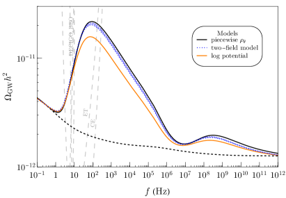
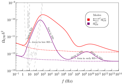
Figure 12: Left: An illustration of the model dependence in the stochastic string gravitational wave spectrum. The solid black line is the case where the rotation energy density $\rho_{\theta}$ follows a piecewise scaling $T\lessgtr T_{\rm MK}$ as shown in Fig. 1. The colored curves are for the two-field model (blue) and the logarithmic potential (orange) with evolution demonstrated in Fig. 1. For the two-field model, we show the blue dotted curves for different ratios of the soft masses of the two fields $\bar{P}$ and $P$, $m_{\bar{P}}/m_{P}=1,100$. The dashed black curve shows the standard string spectrum in a $\Lambda$CDM cosmology. We fix ($T_{\rm KR},T_{\rm RM})=(1\,{\rm GeV},100\,{\rm GeV})$. Right: An illustration of the difference between the $m=1$ amplitude (purple) and the total amplitude summed over $10^{4}$ harmonics (red). The sum over high modes partially flattens the right side of the kination induced peak, shifting the spectral dependence from $f^{-1}$ to $f^{-1/3}$. We fix ($T_{\rm KR},T_{\rm RM})=(1\ {\rm GeV},10\ {\rm TeV})$. In both panels, the second, smaller triangle at high frequencies is an additional fingerprint of axion kination and arises from loops that form in the early radiation dominated era and decay in the subsequent matter or kination dominated eras (see Table 1). Both panels assume $G\mu=5\times 10^{-15}$, and $\alpha=0.1$.

The left panel of Fig. 12 shows the imprint of the saxion potential on the stochastic string gravitational wave background. The black curve corresponds to the piecewise approximation of the $\rho_{\theta}$ contribution to the Hubble rate as used in Eq. (5.14). The blue dotted and orange solid lines show the spectrum for the two-field model and the log potential, respectively. Similar to the gravitational wave spectrum of Fig. 7 for inflation, the spectrum for the two-field model is close to that for the piecewise approximation, while that for the log potential deviates from them. In what follows, we use the piecewise approximation of $\rho_{\theta}$.

The right panel of Fig. 12 illustrates two key features that axion kination imparts to the stochastic string gravitational wave background. First, the purple curves show the $m=1$ contribution to the spectrum, $\Omega_{\rm GW}^{(1)}$, while the red curves shows $\Omega_{\rm GW}$ after summing over $10^{4}$ harmonics. For the $m=1$ amplitude, the triangular shaped peak approaches the expected $f^{-1}$ rise and $f^{1}$ fall as shown in Table 1. The amplitude summed over $10^{4}$ modes, however, demonstrates how the total amplitude deviates from the $m=1$ amplitude. Summing over higher harmonics increases the amplitude roughly by a factor of $\zeta(4/3)$, and most importantly, the contribution from the higher harmonics changes the $f^{-1}$ tail on the right side of the kination induced triangle into a much shallower $f^{-1/3}$ tail while leaving the $f^{1}$ decay on the left side the triangle the same. Such a long and shallow UV tail allows high frequency gravitational wave detectors to discern axion kination from the standard $\Lambda$CDM spectrum even when the triangular kination peak is at much lower frequencies. In addition, a second key feature of axion kination is shown in the second, smaller triangle at higher frequencies compared to the main triangle. The second triangular bump in the spectrum arises from loops that form in the early radiation dominated era prior to kination, and decay in the matter, kination, or late radiation era. As seen from Table 1, loops that form in the early radiation era and decay in these other eras are expected to exhibit a shallower rise and fall in amplitude akin to the main triangular shaped enhancement from loops that form in the matter or kination eras. For sufficiently short eras of kination and matter domination, the smaller, second bump is visible even after summing over higher harmonics. For long eras of kination, the sum over higher harmonics can merge the main kination induced peak with this smaller second peak, as shown for instance, in the purple curves in the left panel of Fig. 13. Nevertheless, the slightly broken power law near $10^{3}$ Hz for the solid purple and $10^{5}$ Hz for the lighter purple contour is a remnant left over from this second triangular peak. The observation of a broken decaying power law or the second triangular bump itself may provide a unique gravitational wave fingerprint for axion induced kination.

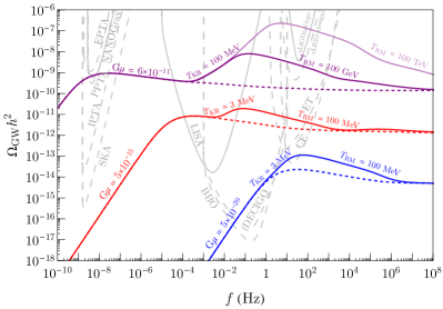
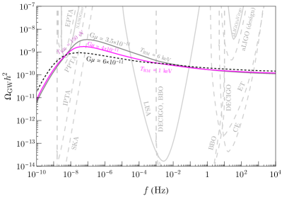
Figure 13: Representative spectra of primordial gravitational waves emitted from local cosmic strings experiencing axion kination (solid) and the standard $\Lambda$CDM cosmology (dashed). Long eras of kination exhibit greater amplitudes in the triangular shaped peak of $\Omega_{\rm GW}h^{2}$, which is a key signature of axion kination. Of crucial importance is the slowly decaying high frequency tail arising from the sum over high mode numbers which enables detectors like BBO, DECIGO, and CE to detect deviations from the $\Lambda$CDM spectrum even when the kination peak is not located within their frequency domain. Left: Early axion kination cosmology where kination occurs before BBN. The top most contour shows the gravitational wave amplitude when $G\mu$ is fixed to pass through the NANOGrav signal. Right: Late axion kination cosmology where kination occurs in the epoch between CMB and BBN. For each contour, we plot the required $G\mu$ to pass through the NANOGrav signal.

Fig. 13 shows the typical gravitational wave spectrum for a stochastic string background experiencing axion kination. Here, we numerically compute (5.4) up to $10^{4}$ modes and fix $\alpha=0.1$ in accordance with simulations Blanco-Pillado and Olum (2017); Blanco-Pillado et al. (2014). The solid contours show $\Omega_{\rm GW}h^{2}$ in the modified axion kination cosmology for a variety of $\{T_{\rm KR},T_{\rm MK},T_{\rm RM}\}$, while the dashed contours show the amplitude in the standard $\Lambda$CDM cosmology. The left and right panels of Fig. 13 represent the expected spectral shape for early and late axion kination eras, respectively. We define early (late) axion kination cosmologies as those that end before (after) BBN. To be consistent with BBN and CMB bounds, this entails that $T_{\rm KR}\gtrsim\,2.5\,{\rm MeV}$ for early axion kination cosmologies and that $130\,{\rm eV}\lesssim T_{\rm KR}\leq T_{\rm RM}\lesssim 6\,{\rm keV}$ for late kination cosmologies as discussed in Sec. 3.

The free parameters $\{G\mu,\alpha,T_{\rm KR},T_{\rm MK}\}$ set the spectral shape of the stochastic background. Independent of the axion kination cosmology, larger $G\mu$ and $\alpha$ elevate the overall amplitude of the spectrum such that the base amplitude of the kination induced triangle scales as $\Omega_{\rm GW,\rm base}h^{2}\simeq 2\times 10^{-4}\sqrt{G\mu\,\alpha}$ for $\alpha\gtrsim\Gamma G\mu$ Blasi et al. (2020). On the other hand, the parameters $T_{\rm KR}$ and $T_{\rm MK}$ determine the size and location of the triangular ‘bump’ with a larger peak corresponding to longer duration of kination and occurring at a higher frequency the greater $T_{\rm MK}$ is. For example, the solid and light purple contours on the left panel of Fig. 13 illustrate the growth and blueshift of the kination induced peak when the duration of the kination era increases for fixed $G\mu$ and $T_{\rm{KR}}$. The red and blue contours in the same panel illustrate the overall decrease in amplitude and the blueshift of the spectrum when lowering $G\mu$ for a fixed duration of kination. In addition, the purple and red contours ($G\mu=6\times 10^{-11}$ and $5\times 10^{-15}$, respectively) illustrate that an era of axion induced kination provides future detectors such as LISA with an excellent opportunity to measure the significant deviation from the standard string spectrum (dashed) over a wide range of $G\mu$ and $(T_{\rm KR},T_{\rm MK}$). Moreover, an axion induced kination cosmology may provide the only way to detect extremely small string tensions in future detectors like BBO and CE as shown by the blue contour ($G\mu=5\times 10^{-20}$).

Similarly, the right panel of Fig. 13 shows the modified gravitational wave spectrum for late kination cosmologies. Here we show a collection of spectra that pass through the observed NANOGrav signal Arzoumanian et al. (2020) that are consistent with CMB and BBN constraints. The dashed black contour shows $\Omega_{\rm GW}h^{2}$ for the standard $\Lambda$CDM cosmology Blasi et al. (2021); Ellis and Lewicki (2021) while the gray contour ($G\mu=3.5\times 10^{-11}$) shows $\Omega_{\rm GW}h^{2}$ for the maximum allowed $T_{\rm RM}$ ($6\,{\rm keV})$ and near the minimum allowed $T_{\rm KR}$ ($130\,{\rm eV})$, producing the largest kination peak passing through NANOGrav that is consistent with CMB and BBN. As $T_{\rm KR}$ and $T_{\rm RM}$ converge and the kination era decreases in duration, $\Omega_{\rm GW}h^{2}$ converges with the standard result, shown, for example, by the magenta contour ($G\mu=4.0\times 10^{-11}$). Fig. 13 demonstrates that a striking difference can exist between $\Omega_{\rm GW}h^{2}$ in the axion kination cosmologies and the standard $\Lambda$CDM cosmology.

To understand the connection between the experimental detection of axion kination via string gravitational waves and axion kination parameters, we first reduce the four dimensional parameter space $\{G\mu,\alpha,T_{\rm KR},T_{\rm MK}\}$ into a simpler two dimensional space of $T_{\rm KR}$ and $T_{\rm MK}$. This is achieved by fixing $G\mu$ so that the gravitational wave amplitude in the modified cosmology passes through the NANOGrav signal $(\Omega_{\rm GW}h^{2},f)\simeq(7.5\times 10^{-10},\,5.2\times 10^{-9}\,{\rm Hz})$) Arzoumanian et al. (2020) , and fixing $\alpha=0.1$ which best matches simulations. For early kination cosmologies (left panel of Fig. 13), this requires $G\mu\simeq 6\times 10^{-11}$. For late kination cosmologies (right panel Fig. 13), which generally exhibit a ‘bump’ in the spectrum at nanohertz frequencies, we decrease $G\mu$ for a given $(T_{\rm KR},T_{\rm MK})$ so that $\Omega_{\rm GW}h^{2}$ still crosses through the NANOGrav signal. The left panel of Fig. 14 demonstrates this effect by showing the necessary $G\mu$ to match the NANOGrav signal in the ($T_{\rm KR}$ $T_{\rm RM}$) plane. For relative long durations of kination ($T_{\rm RM}\gg T_{\rm KR}$), the necessary $G\mu$ decreases by a factor of a few to near $G\mu=3\times 10^{-11}$ (blue region) whereas in the limit of no kination ($T_{\rm RM}\ll T_{\rm KR}$), the necessary $G\mu$ asymptotes to its $\Lambda$CDM value of $6\times 10^{-11}$ (red region).

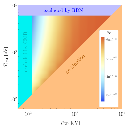
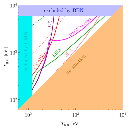
Figure 14: Left: Required $G\mu$ for $\Omega_{\rm GW}h^{2}$ to pass through the NANOGrav signal Arzoumanian et al. (2020); Blasi et al. (2021); Ellis and Lewicki (2021). For long kination eras, which occur when $T_{\rm RM}\gg T_{\rm KR}$, $G\mu$ decreases with respect to the standard $\Lambda$CDM cosmology so that the kination peak does not exceed the NANOGrav signal. Right : The parameter region of axion kination whose imprints on the gravitational wave spectrum from cosmic strings can be detected. For each ($T_{\rm RM},T_{\rm KR})$, we fix $G\mu$ according to the left panel so that spectrum passes through the NANOGrav signal. For the reference $\Lambda$CDM cosmology, we fix $G\mu$ and $\alpha$ to $6\times 10^{-11}$ and $0.1$, respectively, to also fit NANOGrav. For a given $(T_{\rm KR},T_{\rm MK})$, a detection is registered when the difference in amplitudes, $\Omega_{\rm GW}-\Omega_{\rm GW,0}$ is greater than $10\%$ (solid) or 100% (dashed) of the standard cosmological amplitude, $\Omega_{\rm GW,0}$, within the sensitivity curve of the detector.

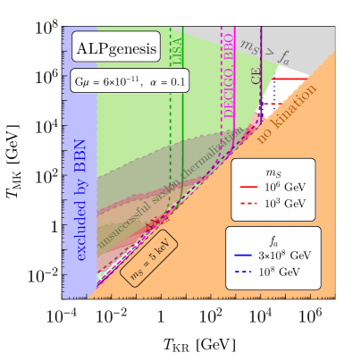
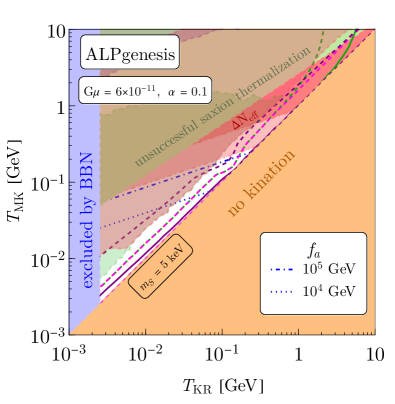
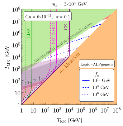
Figure 15: Detector reach of the kination cosmic string gravitational wave spectrum for a range of $T_{\rm KR}$ and $T_{\rm MK}$ consistent with minimal ALPgenesis (top) and lepto-ALPgenesis (bottom). The top-right panel zooms in on the bottom-left part of the top-left panel. $G\mu$ and $\alpha$ are fixed at $6\times 10^{-11}$ and $0.1$, respectively, to fit the NANOGrav data Arzoumanian et al. (2020). For a given $(T_{\rm KR},T_{\rm MK})$, a detection is registered when the difference in amplitudes, $\Omega_{\rm GW}-\Omega_{\rm GW,0}$ is greater than $10\%$ (solid) or 100% (dashed) of the standard cosmological amplitude, $\Omega_{\rm GW,0}$, within the sensitivity curve the detector. In the transparent shared regions, the peak of the spectrum originated from axion kination can be detected.

For a given $(T_{\rm KR},T_{\rm MK})$, we register a detection of axion kination in a similar manner to the “turning-point” prescription of Gouttenoire et al. (2020): First, $\Omega_{\rm GW}h^{2}$ must be greater than the threshold for detection in a given experiment. Second, to actually distinguish between $\Omega_{\rm GW}h^{2}$ in the axion cosmology and the $\Lambda$CDM cosmology, we require that their percent relative difference be greater than a certain threshold within the frequency domain of the experiment. Following Gouttenoire et al. (2020), we take this threshold at a realistic 10% and a more conservative 100% relative difference.

The right panel of Fig. 14 shows the parameter space in the $(T_{\rm KR},T_{\rm RM})$ plane where late axion kination can be detected and distinguished from the standard cosmology with difference of 10% (solid) and 100% (dashed) in $\Omega_{\rm GW}h^{2}$. Here we choose $G\mu$ for each point according to the left panel for axion kination cosmology and take $G\mu=6\times 10^{-11}$ for the standard cosmology. For most of the parameter space consistent with CMB and BBN, an era of kination can be detected and distinguished from the standard cosmological stochastic string background. In addition to the change of the required value of $G\mu$, remarkably, the slowly decaying $f^{-1/3}$ tail originating from the sum over high frequency harmonics, as shown for example by the right panel of Fig. 13, allows detectors like LISA, BBO, DECIGO, and CE to detect late axion kination cosmology. Future detectors like SKA can probe the nanohertz triangular bump. For sufficiently low $T_{\rm KR}$ and high $T_{\rm RM}$, a kination signal may already be observable or excluded at NANOGrav.

Early axion kination is consistent with axiogenesis above the electroweak scale, and can be probed by laser interferometers. We show the constraints on the parameter space of minimal ALPgenesis together with the detection prospects in the upper panels of Fig. 15. The top-right panel zooms in on the bottom-left part of the top-left panel. The slowly decaying $f^{-1/3}$ tail allows detectors like LISA, BBO, DECIGO, and CE to distinguish an early era of axion cosmology for most $T_{\rm KR}\in(10^{-3}\,{\rm GeV},5\times 10^{4}\,{\rm GeV})$. For $T_{\rm KR}\gtrsim 5\times 10^{4}\,{\rm GeV}$, the kination spectrum merges with the standard spectrum at frequencies above $f\gtrsim 10^{3}$ Hz, thereby evading detection. Still, a good portion of the parameter space with $f_{a}\lesssim 10^{8}$ GeV can imprint signals that are detectable by future observations. Future gravitational wave detectors that can observe super-kilohertz frequencies can potentially probe earlier eras of axion kination and hence larger $f_{a}$. In the transparent shaded region, the peak of the spectrum produced by axion kination can be detected. As we argued, this is a smoking-gun signature of axion kination and the detailed shape of the peak contains information about the shape of the potential of the complex field that breaks the $U(1)$ symmetry. The lower two panels of Fig. 15 show the constraints and prospects for lepto-ALPgenesis, for values of $m_{S}$ used in Fig. 11. Future laser interferometers can probe much of the parameter region with low $f_{a}\lesssim 10^{8}$ GeV.

6 Summary and discussion

Axion fields, due to their lightness, may have rich dynamics in the early universe. In this paper, we considered rotations of an axion in field space that naturally provide kination domination preceded by matter domination, which we call axion kination. This non-standard evolution affects the spectrum of possible gravitational waves produced in the early universe. To be concrete, we investigated gravitational waves from inflation and local cosmic strings, which have a nearly flat spectrum when they begin oscillations or are produced during radiation domination. We found that kination domination preceded by matter domination induces a triangular peak in the gravitational wave spectrum.

We studied the theory for axion kination, which involves an approximately quadratic potential for the radial mode and has three parameters: the mass of the radial mode, the axion decay constant, and the comoving charge density. We derived constraints on this parameter space from successful thermalization of the radial mode, BBN, and the CMB. We found large areas of fully realistic parameter space where the theory yields axion kination. The allowed region splits into two pieces, one having early kination domination before BBN and the other having late kination after BBN but well before the CMB last scattering.

Introducing a mass for the axion, we found that part of the axion kination parameter space is consistent with axion dark matter by the kinetic misalignment mechanism while part is not, due to the warmness constraint on dark matter. Similarly, we showed that part of the axion kination parameter space is consistent with generating the baryon asymmetry by ALPgenesis. Furthermore, there are constrained regions with ALP cogenesis yielding both dark matter and the baryon asymmetry, and also regions with the baryon asymmetry successfully generated by lepto-ALPgenesis.

As demonstrated in Sec. 5, axion kination modifies the spectrum of possible primordial gravitational waves through the modification of the expansion history of the universe. By analyzing the spectrum, we can in principle determine the product of the radial mode mass $m_{S}$ and the decay constant $f_{a}$ using the relations given in Eqs. (2.8), (2.9), and (2.10). By further determining $f_{a}$ from axion searches, we may obtain $m_{S}$. In the simplest scenario of gravity mediation in supersymmetry, $m_{S}$ is as large as the masses of the gravitino and scalar partners of Standard Model particles; in other words, we can determine the scale of supersymmetry breaking.

We can further narrow down the parameter space by requiring that the baryon asymmetry of the universe be created from the axion rotation. As shown in Sec. 4.2, this imposes an extra relation on $(m_{S},f_{a})$, and in conjunction with the gravitational wave spectrum, we may make a prediction on both $f_{a}$ and $m_{S}$, which could be confirmed or excluded by measuring $f_{a}$ in axion experiments or $m_{S}$ in collider experiments assuming that $m_{S}$ is tied to the masses of the scalar partners of Standard Model particles.

If the inflation scale is not much below the current upper bound, future observation of gravitational waves can detect the spectrum modified by axion kination, or even the peak of the spectrum that contains information on the shape of the potential of the $U(1)$ symmetry breaking field. In particular, if the QCD axion accounts for dark matter via the kinetic misalignment mechanism, a modification of the gravitational wave spectrum is predicted at high frequencies, $f\gtrsim 10^{-2}$ Hz, as shown in Fig. 8. In this case it is very interesting that this gravitational wave signal can be detected by DECIGO and BBO over most of the allowed parameter space, as shown in Fig. 9; in a significant fraction of the parameter space the gravitational wave peak will be probed. Furthermore, a signal may also be seen at CE if the inflation scale is very near the current upper bound or the sensitivity of CE is improved.

For gravitational waves from cosmic strings, for fixed axion kination cosmology parameters, the modification of the spectrum is predicted at higher frequency, so the QCD axion will not affect the spectrum observable by near future planned experiments. ALPs can affect the spectrum in an observable frequency range.

Gravitational waves from cosmic strings provide signals that can probe axion kination over a wide range of $G\mu$, $T_{\rm{RM}}$ and $T_{\rm{KR}}$, as illustrated in Fig. 13. We examined cosmic strings with a tension suggested by NANOGrav in detail. If axion kination occurs before BBN, the NANOGrav signal can be fitted by the same cosmic strings parameters as in standard cosmology. Importantly, axion kination enhances the spectrum at higher frequencies, allowing laser interferometers to probe the kination era. The enhancement can occur in the parameter region consistent with axiogenesis scenarios, as shown in Fig. 15. If axion kination occurs after BBN, the NANOGrav signal is fitted by a smaller string tension, as shown in the left panel of Fig. 14, and a detailed examination of the spectrum will determine if axion kination is involved. The spectrum at higher frequencies is suppressed, which can be detected by laser interferometers in the parameter region shown in the right panel of Fig. 14.

Our kination era is preceded by an epoch of matter domination that ends without creating entropy. Therefore, matter and kination domination can occur even after BBN. This allows for enhancements to the matter spectrum on small scales that may be probed by observations of Lyman-$\alpha$ and 21 cm lines. Evolving the enhanced matter power spectrum into the non-linear regime and understanding its effects on the Lyman-$\alpha$ flux spectrum as well as hierarchical galaxy formation, and constraints arising from corresponding observations will be discussed in future work.

In this paper, we concentrated on gravitational waves produced by inflation or local cosmic strings and modified by axion kination. At any temperature with early matter or kination domination, the Hubble scale is larger than with radiation domination, and hence, quite generally, primordial gravitational waves are enhanced by axion kination. Furthermore, a distinctive feature appears in the spectrum, a peak or bump depending on the field potential, containing information that probes in detail the era of kination and its origin. It will be interesting to investigate other sources of primordial gravitational waves.

Note added. Soon after the current manuscript was announced on the arXiv, Ref. Gouttenoire et al. (2021) appeared as well. While our analyses have been conducted independently, Ref. Gouttenoire et al. (2021) also discovered the triangular peak signature of axion kination in the spectrum of the primordial gravitational waves from inflation.

Appendix A Evolution of the energy density of axion rotations

In this appendix, we derive the evolution of the axion rotations for the nearly quadratic potentials.

A.1 Logarithmic potential

We first consider the logarithmic potential in Eq. (2.4). The evolution of the axion rotations for this potential is derived in Ref. Co and Harigaya (2020).

We are interested in the rotation dynamics when the Hubble expansion is negligible, $m_{S}\gg H$. In this case, we may obtain short-time scale dynamics ignoring the Hubble expansion and include it when we derive the scaling in a long cosmic time scale. We are also interested in the circular motion after thermalization. Under these assumptions, we may put $\ddot{S}=\dot{S}=0$, and the equation of motion of $S$ requires that

$$\dot{\theta}^{2}=\frac{V^{\prime}(S)}{S}=m_{S}^{2}{\rm ln}\frac{S^{2}}{f_{a}^{2}}.$$ (A.1)

The equation of motion of $\theta$ gives a conservation law of the angular momentum in the field space up to cosmic expansion,

$$n_{\theta}=\dot{\theta}S^{2}=m_{S}S^{2}\left({\rm ln}\frac{S^{2}}{f_{a}^{2}}\right)^{1/2}\propto a^{-3}.$$ (A.2)

Using these two equations, we may obtain the dependence of $S$ and $\dot{\theta}$ on the scale factor $a$,

$$S^{2}=S_{i}^{2}\frac{a_{i}^{3}}{a^{3}}2\sqrt{\frac{{\rm ln}S_{i}/f_{a}}{W(\frac{4a_{i}^{6}S_{i}^{4}{\rm ln}(S_{i}/f_{a})}{a^{6}f_{a}^{4}})}},$$

$$\dot{\theta}^{2}=\frac{1}{2}m_{S}^{2}W(\frac{4a_{i}^{6}S_{i}^{4}{\rm ln}(S_{i}/f_{a})}{a^{6}f_{a}^{4}}),$$ (A.3)

where $W$ is the Lambert $W$ function and $S_{i}$ is an initial field value at a scale factor of $a_{i}$. When $S_{i}\gg f_{a}$ and $a$ is not much above $a_{i}$, $S^{2}\propto a^{-3}$ and $\dot{\theta}$ is nearly a constant. For $a\gg a_{i}$, $S\simeq f_{a}$ and $\dot{\theta}\propto a^{-3}$.

The dependence of the energy density

$$\rho_{\theta}=\frac{1}{2}\dot{\theta}^{2}S^{2}+\frac{1}{2}m_{S}^{2}S^{2}\left({\rm ln}\frac{S^{2}}{f_{a}^{2}}-1\right)+\frac{1}{2}m_{S}^{2}f_{a}^{2}$$ (A.4)

can be obtained by using Eq. (A.1). One can then show that the dependence of $\rho_{\theta}$ on the scale factor $a$ is

$$\frac{d\ln\rho_{\theta}}{d\ln a}=\frac{-6\left(\frac{S}{f_{a}}\right)^{2}\ln\left(\frac{S^{2}}{f_{a}^{2}}\right)}{1-\left(\frac{S}{f_{a}}\right)^{2}+2\left(\frac{S}{f_{a}}\right)^{2}\ln\left(\frac{S^{2}}{f_{a}^{2}}\right)}=\begin{cases}-3&:S\gg f_{a}\\ -6&:S\simeq f_{a}.\end{cases},$$ (A.5)

so at early times, $S\gg f_{a}$, the rotation behaves as matter $\rho_{\theta}\propto a^{-3}$, while at late times, $S\simeq f_{a}$, the rotation behaves as kination $\rho_{\theta}\propto a^{-6}$. This behavior is seen in the orange curve of Fig. 1.

A.2 Two-field model

We next consider the two-field model in Eq. (2.5). We assume that the saxion field value is much larger than the soft masses, so that we may integrate out a linear combination of $P$ and $\bar{P}$ that is paired with $X$ and obtain a mass $\sim S$. Using the constraint $\bar{P}=v_{P}^{2}/P$, from the kinetic and mass terms of $P$ and $\bar{P}$, we obtain an effective Lagrangian

$${\cal L}=\left(1+\frac{v_{P}^{4}}{|P|^{4}}\right)|\partial P|^{2}-m_{P}^{2}|P|^{2}\left(1+r_{P}^{2}\frac{v_{P}^{4}}{|P|^{4}}\right),~{}~{}r_{P}\equiv\frac{m_{\bar{P}}}{m_{P}}.$$ (A.6)

The potential has a minimum at $|P|=\sqrt{r_{P}}v_{P}$ when both $m_{P}^{2}$ and $m_{\bar{P}}^{2}$ are positive.

Putting $\ddot{S}=\dot{S}=0$, the equation of motion of $S$ requires that

$$\dot{\theta}^{2}\left(1-\frac{4v_{P}^{4}}{S^{4}}\right)-m_{P}^{2}\left(1-\frac{4r_{P}^{2}v_{P}^{4}}{S^{4}}\right)=0.$$ (A.7)

The equation of motion of $\theta$ gives a conservation of the angular momentum,

$$n_{\theta}=\dot{\theta}S^{2}\left(1+\frac{4v_{P}^{4}}{S^{4}}\right)\propto a^{-3}.$$ (A.8)

Without loss of generality, we assume that $P\gg v_{P}$, i.e., $S\gg v_{P}$ initially. We first consider $r_{P}>1$ ($m_{P}<m_{\bar{P}}$). Eq. (A.7) means

$$\dot{\theta}^{2}=\frac{1-4r_{P}^{2}v_{P}^{4}/S^{4}}{1-4v_{P}^{4}/S^{4}}m_{P}^{2}.$$ (A.9)

When $S\gg v_{P}$, we obtain $\dot{\theta}^{2}\simeq m_{P}^{2}$. As $S$ approaches the minimum $\sqrt{2r_{P}}v_{P}$, $\dot{\theta}$ approaches $0$. The scaling of $S$ can be derived from charge conservation,

$$n_{\theta}=\dot{\theta}S^{2}\left(1+\frac{4v_{P}^{4}}{S^{4}}\right)=m_{P}S^{2}\left(1+\frac{v_{P}^{4}}{S^{4}}\right)\left(1-\frac{4v_{P}^{4}}{S^{4}}\right)^{-1/2}\left(1-\frac{4r_{P}^{2}v_{P}^{4}}{S^{4}}\right)^{1/2}\propto a^{-3}.$$ (A.10)

The scaling of the energy density

$$\rho_{\theta}=\frac{1}{2}S^{2}\dot{\theta}^{2}\left(1+\frac{4v_{P}^{4}}{S^{4}}\right)+\frac{1}{2}m_{P}^{2}S^{2}\left(1+\frac{4r_{P}^{2}v_{P}^{4}}{S^{4}}\right)-2r_{P}m_{P}^{2}v_{P}^{2}$$ (A.11)

can be derived from these two equations. Here a constant term is subtracted from the energy density so that the energy density vanishes at the minimum. The dependence of $\rho_{\theta}$ on the scale factor $a$ is

$$\frac{d\ln\rho_{\theta}}{d\ln a}=\frac{-3\left(1+\left(\frac{S}{\sqrt{2}v_{P}}\right)^{2}\right)\left(1+r_{P}\left(\frac{S}{\sqrt{2}v_{P}}\right)^{4}\right)}{1+r_{P}\left(\frac{S}{\sqrt{2}v_{P}}\right)^{6}}=\begin{cases}-3&:S\gg\sqrt{2}v_{P}\\ -6&:S\simeq\sqrt{2}v_{P}\end{cases},$$ (A.12)

from which we again observe that at early times, $S\gg\sqrt{2}v_{P}$, the rotation behaves as matter $\rho_{\theta}\propto a^{-3}$, whereas at late times, $S\simeq\sqrt{2}v_{P}$, the rotation behaves as kination $\rho_{\theta}\propto a^{-6}$. This evolution is illustrated by the blue curves of Fig. 1 for various values of $r_{P}$.

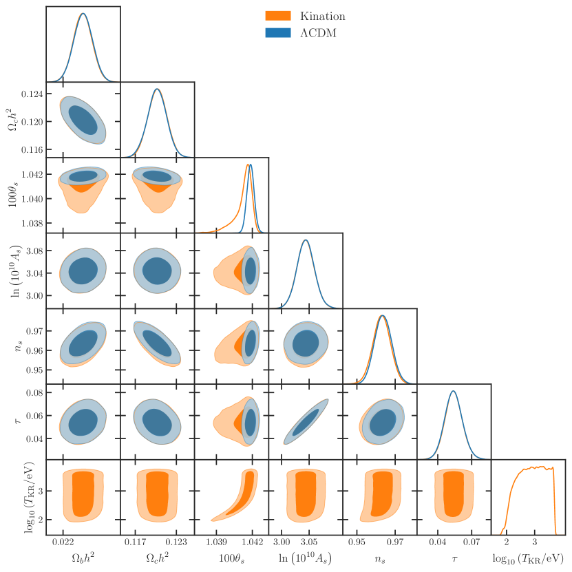
Figure 16: Corner plot for the posterior distributions for the $\Lambda$CDM independent parameters and for the axion kination model. We use the highTTTEEE+lowEE+lowTT likelihood combination from Planck 2018. Contours contain 68% and 95% of the probability.

We next consider $r_{P}=1$. Eq. (A.7) has two solutions, 1) $\dot{\theta}^{2}=m_{P}^{2}$ with $S\neq\sqrt{2}v_{P}$ and 2) $S=\sqrt{2}v_{P}$ with unrestricted $\dot{\theta}$. For $S\gg v_{P}$, the solution is in the branch 1) and gives matter scaling. Charge conservation implies $S^{2}(1+4v_{P}^{4}/S^{4})\propto a^{-3}$. As $S$ decreases according to this scaling and reaches $\sqrt{2}v_{P}$, the branch 2) should be used and charge conservation implies $\dot{\theta}\propto a^{-3}$, giving kination scaling.

Finally, consider $r_{P}<1$. When $S\gg v_{P}$, we again obtain $\dot{\theta}^{2}\simeq m_{P}^{2}$. However, as $S$ approaches $\sqrt{2}v_{P}$ (before reaching the minimum at $\sqrt{2r_{P}}v_{P}$), $\dot{\theta}^{2}$ derived from Eq. (A.9) diverges. This is the point at which the solution becomes unstable. Indeed, when $r_{P}<1$, for a fixed charge, it is energetically favored to have rotations in $\bar{P}$ rather than in $P$, so the rotation dominantly in $P$ is at the most a meta-stable solution. When $S$ reaches $\sqrt{2}v_{P}$, the solution becomes unstable. Quantum tunneling may occur before the instability is reached. We leave the investigation of this scenario to future work and assume $r_{P}\geq 1$.

Appendix B CMB cosmological constrains from Planck

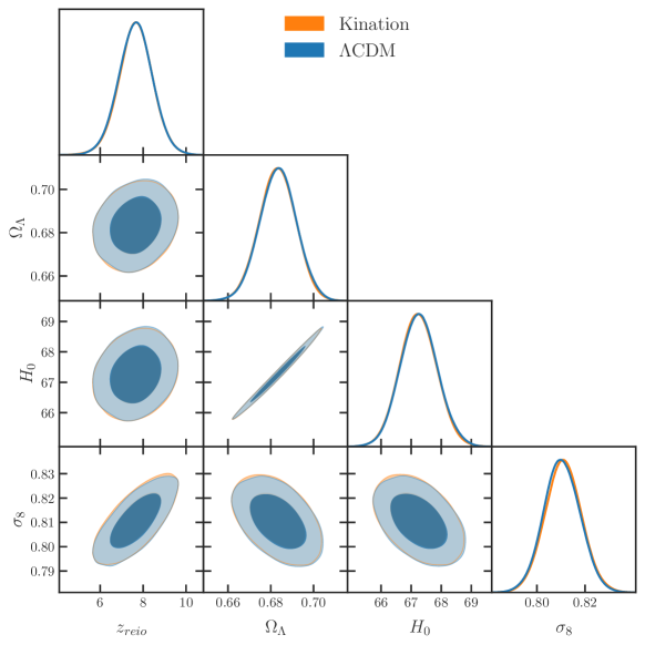
Figure 17: Corner plot for the posterior distributions for the calculated values $\Lambda$CDM parameters and axion kination cosmology. Contours contain 68% and 95% of the probability.

We use a modified version of CLASS Blas et al. (2011) to solve the coupled Boltzmann equations and Monte Python Brinckmann and Lesgourgues (2019) and perform a parameter estimation with the Planck 2018 likelihoods (TT,TE,EE+lowE) data Aghanim et al. (2020b) . Fig. 16 shows the posterior distributions of the six cosmological input parameters for $\Lambda$CDM and the axion kination model: baryon density $\Omega_{b}h^{2}$, DM density $\Omega_{c}h^{2}$, spectral index $n_{s}$, primordial amplitude $A_{s}$, optical depth at reionization $\tau$ and the temperature at kination radiation equality $T_{\rm KR}$. We fix $N_{\rm eff}=3.046$ and assume $\log$ flat prior for $T_{\rm KR}$ between $1\ {\rm eV}\leq T_{\rm KR}\leq 5\ {\rm keV}$. We fix $T_{\rm RM}=5\ {\rm keV}$ and use the identity $T_{\rm MK}^{3}=T_{\rm KR}^{2}T_{\rm RM}$, obtaining $T_{\rm{KR}}>130\,\rm{eV}$ at 95%.

For completeness, Fig. 17 shows the derived parameters: the effective redshift at reionization $z_{reio}$, dark energy density $\Omega_{\Lambda}$, Hubble expansion rate today $H_{0}$, and matter fluctuation amplitude $\sigma_{8}$.

References

- Spokoiny (1993) B. Spokoiny, Phys. Lett. B 315, 40 (1993), arXiv:gr-qc/9306008 .
- Joyce (1997) M. Joyce, Phys. Rev. D 55, 1875 (1997), arXiv:hep-ph/9606223 .
- Visinelli and Gondolo (2010) L. Visinelli and P. Gondolo, Phys. Rev. D 81, 063508 (2010), arXiv:0912.0015 [astro-ph.CO] .
- D’Eramo et al. (2017) F. D’Eramo, N. Fernandez, and S. Profumo, JCAP 05, 012 (2017), arXiv:1703.04793 [hep-ph] .
- Redmond and Erickcek (2017) K. Redmond and A. L. Erickcek, Phys. Rev. D 96, 043511 (2017), arXiv:1704.01056 [hep-ph] .
- D’Eramo et al. (2018) F. D’Eramo, N. Fernandez, and S. Profumo, JCAP 02, 046 (2018), arXiv:1712.07453 [hep-ph] .
- Visinelli (2018) L. Visinelli, Symmetry 10, 546 (2018), arXiv:1710.11006 [astro-ph.CO] .
- Cui et al. (2018) Y. Cui, M. Lewicki, D. E. Morrissey, and J. D. Wells, Phys. Rev. D 97, 123505 (2018), arXiv:1711.03104 [hep-ph] .
- Cui et al. (2019) Y. Cui, M. Lewicki, D. E. Morrissey, and J. D. Wells, JHEP 01, 081 (2019), arXiv:1808.08968 [hep-ph] .
- Bettoni et al. (2019) D. Bettoni, G. Domènech, and J. Rubio, JCAP 02, 034 (2019), arXiv:1810.11117 [astro-ph.CO] .
- Ramberg and Visinelli (2019) N. Ramberg and L. Visinelli, Phys. Rev. D 99, 123513 (2019), arXiv:1904.05707 [astro-ph.CO] .
- Auclair et al. (2020) P. Auclair et al., JCAP 04, 034 (2020), arXiv:1909.00819 [astro-ph.CO] .
- Chang and Cui (2020) C.-F. Chang and Y. Cui, Phys. Dark Univ. 29, 100604 (2020), arXiv:1910.04781 [hep-ph] .
- Gouttenoire et al. (2020) Y. Gouttenoire, G. Servant, and P. Simakachorn, JCAP 07, 032 (2020), arXiv:1912.02569 [hep-ph] .
- Chang and Cui (2021) C.-F. Chang and Y. Cui, (2021), arXiv:2106.09746 [hep-ph] .
- Giovannini (1998) M. Giovannini, Phys. Rev. D 58, 083504 (1998), arXiv:hep-ph/9806329 .
- Giovannini (1999a) M. Giovannini, Phys. Rev. D 60, 123511 (1999a), arXiv:astro-ph/9903004 .
- Giovannini (1999b) M. Giovannini, Class. Quant. Grav. 16, 2905 (1999b), arXiv:hep-ph/9903263 .
- Riazuelo and Uzan (2000) A. Riazuelo and J.-P. Uzan, Phys. Rev. D 62, 083506 (2000), arXiv:astro-ph/0004156 .
- Sahni et al. (2002) V. Sahni, M. Sami, and T. Souradeep, Phys. Rev. D 65, 023518 (2002), arXiv:gr-qc/0105121 .
- Tashiro et al. (2004) H. Tashiro, T. Chiba, and M. Sasaki, Class. Quant. Grav. 21, 1761 (2004), arXiv:gr-qc/0307068 .
- Boyle and Buonanno (2008) L. A. Boyle and A. Buonanno, Phys. Rev. D 78, 043531 (2008), arXiv:0708.2279 [astro-ph] .
- Giovannini (2010) M. Giovannini, PMC Phys. A 4, 1 (2010), arXiv:0901.3026 [astro-ph.CO] .
- Kuroyanagi et al. (2011) S. Kuroyanagi, K. Nakayama, and S. Saito, Phys. Rev. D 84, 123513 (2011), arXiv:1110.4169 [astro-ph.CO] .
- Li et al. (2017) B. Li, P. R. Shapiro, and T. Rindler-Daller, Phys. Rev. D 96, 063505 (2017), arXiv:1611.07961 [astro-ph.CO] .
- Kuroyanagi et al. (2018) S. Kuroyanagi, T. Chiba, and T. Takahashi, JCAP 11, 038 (2018), arXiv:1807.00786 [astro-ph.CO] .
- Bernal and Hajkarim (2019) N. Bernal and F. Hajkarim, Phys. Rev. D 100, 063502 (2019), arXiv:1905.10410 [astro-ph.CO] .
- Figueroa and Tanin (2019) D. G. Figueroa and E. H. Tanin, JCAP 08, 011 (2019), arXiv:1905.11960 [astro-ph.CO] .
- Dalianis and Kritos (2021) I. Dalianis and K. Kritos, Phys. Rev. D 103, 023505 (2021), arXiv:2007.07915 [astro-ph.CO] .
- Hook et al. (2021) A. Hook, G. Marques-Tavares, and D. Racco, JHEP 02, 117 (2021), arXiv:2010.03568 [hep-ph] .
- Li and Shapiro (2021) B. Li and P. R. Shapiro, (2021), arXiv:2107.12229 [astro-ph.CO] .
- Redmond et al. (2018) K. Redmond, A. Trezza, and A. L. Erickcek, Phys. Rev. D 98, 063504 (2018), arXiv:1807.01327 [astro-ph.CO] .
- Visinelli and Redondo (2020) L. Visinelli and J. Redondo, Phys. Rev. D 101, 023008 (2020), arXiv:1808.01879 [astro-ph.CO] .
- Co and Harigaya (2020) R. T. Co and K. Harigaya, Phys. Rev. Lett. 124, 111602 (2020), arXiv:1910.02080 [hep-ph] .
- Co et al. (2020a) R. T. Co, L. J. Hall, and K. Harigaya, Phys. Rev. Lett. 124, 251802 (2020a), arXiv:1910.14152 [hep-ph] .
- Peccei and Quinn (1977a) R. D. Peccei and H. R. Quinn, Phys. Rev. Lett. 38, 1440 (1977a).
- Peccei and Quinn (1977b) R. D. Peccei and H. R. Quinn, Phys. Rev. D 16, 1791 (1977b).
- Weinberg (1978) S. Weinberg, Phys. Rev. Lett. 40, 223 (1978).
- Wilczek (1978) F. Wilczek, Phys. Rev. Lett. 40, 279 (1978).
- Arzoumanian et al. (2020) Z. Arzoumanian et al. (NANOGrav), Astrophys. J. Lett. 905, L34 (2020), arXiv:2009.04496 [astro-ph.HE] .
- Ellis and Lewicki (2021) J. Ellis and M. Lewicki, Phys. Rev. Lett. 126, 041304 (2021), arXiv:2009.06555 [astro-ph.CO] .
- Blasi et al. (2021) S. Blasi, V. Brdar, and K. Schmitz, Phys. Rev. Lett. 126, 041305 (2021), arXiv:2009.06607 [astro-ph.CO] .
- Affleck and Dine (1985) I. Affleck and M. Dine, Nucl. Phys. B 249, 361 (1985).
- Moxhay and Yamamoto (1985) P. Moxhay and K. Yamamoto, Phys. Lett. B 151, 363 (1985).
- Co et al. (2021a) R. T. Co, N. Fernandez, A. Ghalsasi, L. J. Hall, and K. Harigaya, JHEP 03, 017 (2021a), arXiv:2006.05687 [hep-ph] .
- Mukaida and Nakayama (2013) K. Mukaida and K. Nakayama, JCAP 01, 017 (2013), arXiv:1208.3399 [hep-ph] .
- Co et al. (2021b) R. T. Co, K. Harigaya, and A. Pierce, (2021b), arXiv:2104.02077 [hep-ph] .
- Fields et al. (2020) B. D. Fields, K. A. Olive, T.-H. Yeh, and C. Young, JCAP 03, 010 (2020), [Erratum: JCAP 11, E02 (2020)], arXiv:1912.01132 [astro-ph.CO] .
- Arbey (2012) A. Arbey, Comput. Phys. Commun. 183, 1822 (2012), arXiv:1106.1363 [astro-ph.CO] .
- Arbey et al. (2020) A. Arbey, J. Auffinger, K. P. Hickerson, and E. S. Jenssen, Comput. Phys. Commun. 248, 106982 (2020), arXiv:1806.11095 [astro-ph.CO] .
- Aghanim et al. (2020a) N. Aghanim et al. (Planck), Astron. Astrophys. 641, A6 (2020a), [Erratum: Astron.Astrophys. 652, C4 (2021)], arXiv:1807.06209 [astro-ph.CO] .
- Zyla et al. (2020) P. A. Zyla et al. (Particle Data Group), PTEP 2020, 083C01 (2020).
- Blas et al. (2011) D. Blas, J. Lesgourgues, and T. Tram, JCAP 07, 034 (2011), arXiv:1104.2933 [astro-ph.CO] .
- Brinckmann and Lesgourgues (2019) T. Brinckmann and J. Lesgourgues, Phys. Dark Univ. 24, 100260 (2019), arXiv:1804.07261 [astro-ph.CO] .
- Preskill et al. (1983) J. Preskill, M. B. Wise, and F. Wilczek, Phys. Lett. B 120, 127 (1983).
- Abbott and Sikivie (1983) L. Abbott and P. Sikivie, Phys. Lett. B 120, 133 (1983).
- Dine and Fischler (1983) M. Dine and W. Fischler, Phys. Lett. B 120, 137 (1983).
- Dolgov and Kirilova (1990) A. Dolgov and D. Kirilova, Sov. J. Nucl. Phys. 51, 172 (1990).
- Traschen and Brandenberger (1990) J. H. Traschen and R. H. Brandenberger, Phys. Rev. D 42, 2491 (1990).
- Kofman et al. (1994) L. Kofman, A. D. Linde, and A. A. Starobinsky, Phys. Rev. Lett. 73, 3195 (1994), arXiv:hep-th/9405187 .
- Shtanov et al. (1995) Y. Shtanov, J. H. Traschen, and R. H. Brandenberger, Phys. Rev. D 51, 5438 (1995), arXiv:hep-ph/9407247 .
- Kofman et al. (1997) L. Kofman, A. D. Linde, and A. A. Starobinsky, Phys. Rev. D 56, 3258 (1997), arXiv:hep-ph/9704452 .
- Jaeckel et al. (2017) J. Jaeckel, V. M. Mehta, and L. T. Witkowski, JCAP 01, 036 (2017), arXiv:1605.01367 [hep-ph] .
- Berges et al. (2019) J. Berges, A. Chatrchyan, and J. Jaeckel, JCAP 08, 020 (2019), arXiv:1903.03116 [hep-ph] .
- Fonseca et al. (2020) N. Fonseca, E. Morgante, R. Sato, and G. Servant, JHEP 04, 010 (2020), arXiv:1911.08472 [hep-ph] .
- Micha and Tkachev (2003) R. Micha and I. I. Tkachev, Phys. Rev. Lett. 90, 121301 (2003), arXiv:hep-ph/0210202 .
- Micha and Tkachev (2004) R. Micha and I. I. Tkachev, Phys. Rev. D 70, 043538 (2004), arXiv:hep-ph/0403101 .
- Co et al. (2018) R. T. Co, L. J. Hall, and K. Harigaya, Phys. Rev. Lett. 120, 211602 (2018), arXiv:1711.10486 [hep-ph] .
- McLerran et al. (1991) L. D. McLerran, E. Mottola, and M. E. Shaposhnikov, Phys. Rev. D 43, 2027 (1991).
- Co et al. (2020b) R. T. Co, L. J. Hall, K. Harigaya, K. A. Olive, and S. Verner, JCAP 08, 036 (2020b), arXiv:2004.00629 [hep-ph] .
- Iršič et al. (2017) V. Iršič et al., Phys. Rev. D 96, 023522 (2017), arXiv:1702.01764 [astro-ph.CO] .
- Co et al. (2021c) R. T. Co, L. J. Hall, and K. Harigaya, JHEP 01, 172 (2021c), arXiv:2006.04809 [hep-ph] .
- D’Onofrio et al. (2014) M. D’Onofrio, K. Rummukainen, and A. Tranberg, Phys. Rev. Lett. 113, 141602 (2014), arXiv:1404.3565 [hep-ph] .
- Ellis and Olive (1987) J. R. Ellis and K. A. Olive, Phys. Lett. B 193, 525 (1987).
- Raffelt and Seckel (1988) G. Raffelt and D. Seckel, Phys. Rev. Lett. 60, 1793 (1988).
- Turner (1988) M. S. Turner, Phys. Rev. Lett. 60, 1797 (1988).
- Mayle et al. (1988) R. Mayle, J. R. Wilson, J. R. Ellis, K. A. Olive, D. N. Schramm, and G. Steigman, Phys. Lett. B 203, 188 (1988).
- Raffelt (2008) G. G. Raffelt, Lect. Notes Phys. 741, 51 (2008), arXiv:hep-ph/0611350 .
- Payez et al. (2015) A. Payez, C. Evoli, T. Fischer, M. Giannotti, A. Mirizzi, and A. Ringwald, JCAP 02, 006 (2015), arXiv:1410.3747 [astro-ph.HE] .
- Bar et al. (2020) N. Bar, K. Blum, and G. D’Amico, Phys. Rev. D 101, 123025 (2020), arXiv:1907.05020 [hep-ph] .
- Harigaya and Wang (2021) K. Harigaya and R. Wang, (2021), arXiv:2107.09679 [hep-ph] .
- Chakraborty et al. (2021) S. Chakraborty, T. H. Jung, and T. Okui, (2021), arXiv:2108.04293 [hep-ph] .
- Starobinsky (1985) A. A. Starobinsky, Sov. Astron. Lett. 11, 133 (1985).
- Weinberg (2004) S. Weinberg, Phys. Rev. D 69, 023503 (2004), arXiv:astro-ph/0306304 .
- Saikawa and Shirai (2018) K. Saikawa and S. Shirai, JCAP 05, 035 (2018), arXiv:1803.01038 [hep-ph] .
- Schmitz (2021) K. Schmitz, JHEP 01, 097 (2021), arXiv:2002.04615 [hep-ph] .
- McLaughlin (2013) M. A. McLaughlin, Class. Quant. Grav. 30, 224008 (2013), arXiv:1310.0758 [astro-ph.IM] .
- Arzoumanian et al. (2018) Z. Arzoumanian et al. (NANOGRAV), Astrophys. J. 859, 47 (2018), arXiv:1801.02617 [astro-ph.HE] .
- Aggarwal et al. (2019) K. Aggarwal et al., Astrophys. J. 880, 2 (2019), arXiv:1812.11585 [astro-ph.GA] .
- Brazier et al. (2019) A. Brazier et al., (2019), arXiv:1908.05356 [astro-ph.IM] .
- Manchester et al. (2013) R. N. Manchester et al., Publ. Astron. Soc. Austral. 30, 17 (2013), arXiv:1210.6130 [astro-ph.IM] .
- Shannon et al. (2015) R. M. Shannon et al., Science 349, 1522 (2015), arXiv:1509.07320 [astro-ph.CO] .
- Kramer and Champion (2013) M. Kramer and D. J. Champion, Class. Quant. Grav. 30, 224009 (2013).
- Lentati et al. (2015) L. Lentati et al., Mon. Not. Roy. Astron. Soc. 453, 2576 (2015), arXiv:1504.03692 [astro-ph.CO] .
- Babak et al. (2016) S. Babak et al., Mon. Not. Roy. Astron. Soc. 455, 1665 (2016), arXiv:1509.02165 [astro-ph.CO] .
- Hobbs et al. (2010) G. Hobbs et al., Class. Quant. Grav. 27, 084013 (2010), arXiv:0911.5206 [astro-ph.SR] .
- Manchester (2013) R. N. Manchester, Class. Quant. Grav. 30, 224010 (2013), arXiv:1309.7392 [astro-ph.IM] .
- Verbiest et al. (2016) J. P. W. Verbiest et al., Mon. Not. Roy. Astron. Soc. 458, 1267 (2016), arXiv:1602.03640 [astro-ph.IM] .
- Hazboun et al. (2018) J. S. Hazboun, C. M. F. Mingarelli, and K. Lee, (2018), arXiv:1810.10527 [astro-ph.IM] .
- Carilli and Rawlings (2004) C. L. Carilli and S. Rawlings, New Astron. Rev. 48, 979 (2004), arXiv:astro-ph/0409274 .
- Janssen et al. (2015) G. Janssen et al., PoS AASKA14, 037 (2015), arXiv:1501.00127 [astro-ph.IM] .
- Weltman et al. (2020) A. Weltman et al., Publ. Astron. Soc. Austral. 37, e002 (2020), arXiv:1810.02680 [astro-ph.CO] .
- Amaro-Seoane et al. (2017) P. Amaro-Seoane et al. (LISA), (2017), arXiv:1702.00786 [astro-ph.IM] .
- Baker et al. (2019) J. Baker et al., (2019), arXiv:1907.06482 [astro-ph.IM] .
- Crowder and Cornish (2005) J. Crowder and N. J. Cornish, Phys. Rev. D 72, 083005 (2005), arXiv:gr-qc/0506015 .
- Corbin and Cornish (2006) V. Corbin and N. J. Cornish, Class. Quant. Grav. 23, 2435 (2006), arXiv:gr-qc/0512039 .
- Harry et al. (2006) G. M. Harry, P. Fritschel, D. A. Shaddock, W. Folkner, and E. S. Phinney, Class. Quant. Grav. 23, 4887 (2006), [Erratum: Class.Quant.Grav. 23, 7361 (2006)].
- Seto et al. (2001) N. Seto, S. Kawamura, and T. Nakamura, Phys. Rev. Lett. 87, 221103 (2001), arXiv:astro-ph/0108011 .
- Kawamura et al. (2006) S. Kawamura et al., Class. Quant. Grav. 23, S125 (2006).
- Yagi and Seto (2011) K. Yagi and N. Seto, Phys. Rev. D 83, 044011 (2011), [Erratum: Phys.Rev.D 95, 109901 (2017)], arXiv:1101.3940 [astro-ph.CO] .
- Abbott et al. (2017) B. P. Abbott et al. (LIGO Scientific), Class. Quant. Grav. 34, 044001 (2017), arXiv:1607.08697 [astro-ph.IM] .
- Reitze et al. (2019) D. Reitze et al., Bull. Am. Astron. Soc. 51, 035 (2019), arXiv:1907.04833 [astro-ph.IM] .
- Punturo et al. (2010) M. Punturo et al., Class. Quant. Grav. 27, 194002 (2010).
- Hild et al. (2011) S. Hild et al., Class. Quant. Grav. 28, 094013 (2011), arXiv:1012.0908 [gr-qc] .
- Sathyaprakash et al. (2012) B. Sathyaprakash et al., Class. Quant. Grav. 29, 124013 (2012), [Erratum: Class.Quant.Grav. 30, 079501 (2013)], arXiv:1206.0331 [gr-qc] .
- Maggiore et al. (2020) M. Maggiore et al., JCAP 03, 050 (2020), arXiv:1912.02622 [astro-ph.CO] .
- Harry (2010) G. M. Harry (LIGO Scientific), Class. Quant. Grav. 27, 084006 (2010).
- Aasi et al. (2015) J. Aasi et al. (LIGO Scientific), Class. Quant. Grav. 32, 074001 (2015), arXiv:1411.4547 [gr-qc] .
- Acernese et al. (2015) F. Acernese et al. (VIRGO), Class. Quant. Grav. 32, 024001 (2015), arXiv:1408.3978 [gr-qc] .
- Abbott et al. (2021) R. Abbott et al. (LIGO Scientific, Virgo), SoftwareX 13, 100658 (2021), arXiv:1912.11716 [gr-qc] .
- Watanabe and Komatsu (2006) Y. Watanabe and E. Komatsu, Phys. Rev. D 73, 123515 (2006), arXiv:astro-ph/0604176 .
- Abazajian et al. (2016) K. N. Abazajian et al. (CMB-S4), (2016), arXiv:1610.02743 [astro-ph.CO] .
- Vachaspati and Vilenkin (1985) T. Vachaspati and A. Vilenkin, Phys. Rev. D 31, 3052 (1985).
- Kibble (1976) T. W. B. Kibble, J. Phys. A 9, 1387 (1976).
- Minkowski (1977) P. Minkowski, Phys. Lett. B 67, 421 (1977).
- Yanagida (1979) T. Yanagida, Conf. Proc. C 7902131, 95 (1979).
- Gell-Mann et al. (1979) M. Gell-Mann, P. Ramond, and R. Slansky, Conf. Proc. C 790927, 315 (1979), arXiv:1306.4669 [hep-th] .
- Mohapatra and Senjanovic (1980) R. N. Mohapatra and G. Senjanovic, Phys. Rev. Lett. 44, 912 (1980).
- Vilenkin and Shellard (2000) A. Vilenkin and E. P. S. Shellard, Cosmic strings and other topological defects (Cambridge University Press, 2000).
- Blanco-Pillado and Olum (2017) J. J. Blanco-Pillado and K. D. Olum, Phys. Rev. D 96, 104046 (2017), arXiv:1709.02693 [astro-ph.CO] .
- Binetruy et al. (2009) P. Binetruy, A. Bohe, T. Hertog, and D. A. Steer, Phys. Rev. D 80, 123510 (2009), arXiv:0907.4522 [hep-th] .
- Blanco-Pillado et al. (2014) J. J. Blanco-Pillado, K. D. Olum, and B. Shlaer, Phys. Rev. D 89, 023512 (2014), arXiv:1309.6637 [astro-ph.CO] .
- Dubath et al. (2008) F. Dubath, J. Polchinski, and J. V. Rocha, Phys. Rev. D 77, 123528 (2008), arXiv:0711.0994 [astro-ph] .
- Blasi et al. (2020) S. Blasi, V. Brdar, and K. Schmitz, Phys. Rev. Res. 2, 043321 (2020), arXiv:2004.02889 [hep-ph] .
- Gouttenoire et al. (2021) Y. Gouttenoire, G. Servant, and P. Simakachorn, (2021), arXiv:2108.10328 [hep-ph] .
- Aghanim et al. (2020b) N. Aghanim et al. (Planck), Astron. Astrophys. 641, A5 (2020b), arXiv:1907.12875 [astro-ph.CO] .