Inelastic Axial and Vector Structure Functions for Lepton-Nucleon Scattering 2021 Update

Abstract

We report on an update (2021) of a phenomenological model for inelastic neutrino- and electron-nucleon scattering cross sections using effective leading order parton distribution functions with a new scaling variable $\xi_{w}$. Non-perturbative effects are well described using the $\xi_{w}$ scaling variable in combination with multiplicative $K$ factors at low $Q^{2}$. The model describes all inelastic charged-lepton-nucleon scattering data (HERA/NMC/BCDMS/SLAC/JLab) ranging from very high $Q^{2}$ to very low $Q^{2}$ and down to the $Q^{2}=0$ photo-production region. The model has been developed to be used in analysis of neutrino oscillation experiments in the few GeV region. The 2021 update accounts for the difference between axial and vector structure function which brings it into much better agreement with neutrino-nucleon total cross section measurements. The model has been developed primarily for hadronic final state masses $W$ above 1.8 GeV. However with additional parameters the model also describe the $average$ neutrino cross sections in the resonance region down to $W$=1.4 GeV.

1 Introduction

The field of neutrino oscillation physics has progressed from the discovery of neutrino oscillation ATM to an era of precision measurements of mass splitting and mixing angles. Uncertainties in modeling the cross sections for neutrino interactions in the few GeV region result in systematic uncertainties in the extraction of mass splitting and mixing parameters in neutrino oscillations experiments such as MINOSMINOS ; MINOS2 , NO$\nu$ANOVA , K2K K2K , SuperKsuperK , T2KT2K , MiniBooNEMiniBooNE , and DUNEDUNE . A reliable model of neutrino inelastic cross sections at low energies is essential for precise neutrino oscillations experiments.

The interest in neutrino interactions at low energies has resulted in the construction of several near detectors (e.g. MINOSMINOS2 , T2KT2K ) to measure low energy cross sections and fluxes, as well as experiments (e.g. SciBooNE sciboone , MicroBooNEMicroBooNE , ArgonNeu argoneut , MINERvAminerva1 ) and ICARUSICARUS at Fermilab which are designed to measure neutrino cross sections at low energies.

In this communication, we report on an update of duality based model of neutrino interactions using effective leading order parton distribution functions (PDFs). Earlier versions of the modelnuint01-2 ; nuint04 have been incorporated into several Monte Carlo generators of neutrino interactions including NEUTNEUT , GENIEGENIE , NEUGENNEUGEN and NUANCENUANCE . The current version of GENIE is using the NUINT04nuint04 version of the model. These early versions assume that the axial structure functions are the same as the vector structure functions.

In this 2021 update, we both further refine the model and $also$ account for the difference between axial and vector structure functions at low values of $Q^{2}$. We refer to the version of the model which assumes that vector and axial structure functions are the same as ”Type I (A=V)”. The ”Type I” version should be used to model electron and muon scattering. We refer to the updated version of the model that accounts for the difference in vector and axial structure functions as ”Type II (A$>$V)”. The ”Type II (A$>$V)” model should be used to model neutrino scattering,

In the few GeV region there are contributions from several kinds of lepton-nucleon interaction processes as defined by the final state invariant mass $W$ and the invariant square of the momentum transfer $Q^{2}$. These include quasi-elastic reactions ($W<1.07~{}GeV$), the $\Delta(1232)$ region ($1.1<W<1.4~{}GeV$ ), higher mass resonances ($1.4<W<1.8~{}GeV$), and the inelastic continuum region ($W>1.8~{}GeV$). At low momentum transfer the inelastic continuum is sometimes referred to as ”shallow inelastic”, and at high momentum transfer it is referred to as ”deep inelastic”. It is quite challenging to disentangle each of those contributions separately, and in particular the contribution of resonance production and the inelastic scattering continuum. At low $Q^{2}$ there are large non-perturbative contributions to the inelastic cross section. These include kinematic target mass corrections, dynamic higher twist effects, higher order Quantum Chromodynamic (QCD) terms, and nuclear effects in nuclear targets.

In this paper we focus on the inelastic part of the cross sections above the region of the $\Delta$(1232) resonance (i.e. the higher mass resonances, and the inelastic continuum). Other models (e.g. vector and axial form factors) should be used describe the quasielastic and $\Delta$(1232) resonance contributions.

In previous studies highx ; nnlo ; yangthesis , we have investigated non-perturbative effects within Leading Order (LO), Next-to-Leading Order (NLO) and Next-to-Next Leading Order (NNLO) QCD using charged-lepton-nucleon scattering experimental data slac ; bcdms ; nmcdata . We found that in NLO QCD, most of the empirical higher-twist terms needed to obtain good agreement with the low energy data for $Q^{2}>$ 1 GeV² originate primarily from target mass effects and the missing NNLO terms (i.e. not from interactions with spectator quarks).

If such is the case, then these terms should be the same in charged-leptons ($e$, $\mu$) and neutrino ($\nu_{\mu}$) scattering. Therefore, the vector part of low energy $\nu_{\mu}$ inelastic cross sections can be described by effective Parton Distribution Functions (PDFs) which are fit to high $Q^{2}$ charged-lepton-nucleon scattering data, but modified to include target mass and higher-twist corrections that are extracted from low energy $e/\mu$ scattering data. For $Q^{2}<$ 1 GeV² additional corrections for non-perturbative effects from spectator quarks are required. These corrections can be parametrized as multiplicative $K$ factors. In neutrino interaction the $K$ factor terms should be the same as in $e/\mu$ scattering for the vector (but not axial) part of the structure functions.

A model that describes electron and muon scattering can then be used to model the vector contribution to neutrino scattering. For large $Q^{2}$ (e.g. $Q^{2}>1$ GeV²) the vector and and axial structure functions are expected to be equal. However, at low $Q^{2}$ the vector and axial structure functions are not equal. The axial structure functions at low values of $Q^{2}$ are not constrained by muon and electron scattering data, because the vector (but not axial) structure functions must go to zero at $Q^{2}$=0. The modeling of the difference between the low $Q^{2}$ vector and axial structure functions requires additional parameters.

In this paper we use CCFR neutrino structure function measurements at low $x$ and low $Q^{2}$ to constrain the low $Q^{2}$ axial $K$ factors for sea quarks, and neutrino total cross section measurements to constrain the low $Q^{2}$ axial $K$ factors for valence quarks.

2 Electron-nucleon and muon-nucleon scattering

In this section we define the kinematic variables for the case of charged-lepton scattering from neutrons and protons. The differential cross section for scattering of an unpolarized charged-lepton with an incident energy $E_{0}$, final energy $E^{\prime}$ and scattering angle $\theta$ can be written in terms of the structure functions ${\cal F}_{1}$ and ${\cal F}_{2}$ as:

$\frac{d^{2}\sigma}{d\Omega dE^{\prime}}(E_{0},E^{\prime},\theta)=\frac{4\alpha^{2}E^{\prime 2}}{Q^{4}}\cos^{2}(\theta/2)$

$\times\left[{\cal F}_{2}(x,Q^{2})/\nu+2\tan^{2}(\theta/2){\cal F}_{1}(x,Q^{2})/M\right],$

where $\alpha$ is the fine structure constant, $M$ is the nucleon mass, $\nu=E_{0}-E^{\prime}$ is energy of the virtual photon which mediates the interaction, $Q^{2}=4E_{0}E^{\prime}\sin^{2}(\theta/2)$ is the invariant four-momentum transfer squared, and the Bjorken variable $x=Q^{2}/2M\nu$ is a measure of the longitudinal momentum carried by the struck partons in a frame in which the proton has high momentum. Here ${\cal F}_{2}=\nu{\cal W}_{2}$, ${\cal F}_{1}=M{\cal W}_{1}$ (and for neutrino scattering ${\cal F}_{3}=\nu{\cal W}_{3}$).

Alternatively, one could view this scattering process as virtual photon absorption. Unlike the real photon, the virtual photon can have two modes of polarization. In terms of the cross section for the absorption of transverse $(\sigma_{T})$ and longitudinal $(\sigma_{L})$ virtual photons, the differential cross section can be written as,

$$\frac{d^{2}\sigma}{d\Omega dE^{\prime}}=\Gamma\left[\sigma_{T}(x,Q^{2})+\epsilon\sigma_{L}(x,Q^{2})\right],$$ (1)

where

$$\Gamma = \frac{\alpha KE^{\prime}}{4\pi^{2}Q^{2}E_{0}}\left(\frac{2}{1-\epsilon}\right)$$ (2)

$$K = \frac{Q^{2}(1-x)}{2Mx}=\frac{2M\nu-Q^{2}}{2M}$$ (3)

$$\epsilon = \left[1+2(1+\frac{Q^{2}}{4M^{2}x^{2}})tan^{2}\frac{\theta}{2}\right]^{-1}.$$ (4)

The quantities $\Gamma$ and $\epsilon$ represent the flux and the degree of longitudinal polarization of the virtual photons respectively. Alternatively we can express $\epsilon$ in terms of the inelasticity $y=\nu/E_{0}$ as follows:

$$\epsilon = \frac{1-y-Q^{2}/(4E_{0}^{2})}{1-y+y^{2}/2+Q^{2}/(4E_{0}^{2})},$$ (5)

which in the limit of $Q^{2}<<E_{0}^{2}$ is approximately

$$\epsilon = \frac{2(1-y)}{2(1-y)+y^{2}}.$$ (6)

Here, $y$ close to zero corresponds to $\epsilon=1$ and $y$ close to one corresponds to $\epsilon=0$.

The quantity ${\cal R}$ is defined as the ratio $\sigma_{L}/\sigma_{T}$, and is related to the structure functions by,

$${\cal R}(x,Q^{2})=\frac{\sigma_{L}}{\sigma_{T}}=\frac{{\cal F}_{2}}{2x{\cal F}_{1}}(1+\frac{4M^{2}x^{2}}{Q^{2}})-1=\frac{{\cal F}_{L}}{2x{\cal F}_{1}},$$ (7)

where ${\cal F}_{L}$ is called the longitudinal structure function. The structure functions are expressed in terms of $\sigma_{L}$ and $\sigma_{T}$ as follows:

$${\cal F}_{1} = \frac{MK}{4\pi^{2}\alpha}\sigma_{T}$$ (8)

$${\cal F}_{2} = \frac{\nu K(\sigma_{L}+\sigma_{T})}{4\pi^{2}\alpha(1+\frac{Q^{2}}{4M^{2}x^{2}})}$$ (9)

$${\cal F}_{L}(x,Q^{2}) = {\cal F}_{2}\left(1+\frac{4M^{2}x^{2}}{Q^{2}}\right)-2x{\cal F}_{1},$$ (10)

or

$$2x{\cal F}_{1}={\cal F}_{2}\left(1+\frac{4M^{2}x^{2}}{Q^{2}}\right)-{\cal F}_{L}(x,Q^{2}).$$ (11)

In addition, $2x{\cal F}_{1}$ is given by

$$2x{\cal F}_{1}(x,Q^{2}) = {\cal F}_{2}(x,Q^{2})\frac{1+4M^{2}x^{2}/Q^{2}}{1+{\cal R}(x,Q^{2})}.$$ (12)

Standard PDFs are extracted from global fits to various sets of deep inelastic (DIS) scattering data at high energies and high $Q^{2}$, where non-perturbative QCD effects are small. PDF fits are performed within the framework of QCD in either LO, NLO or NNLO. Here, using a new scaling variable ($\xi_{w}$) we construct effective LO PDFs that account for the contributions from target mass corrections, non-perturbative QCD effects, and higher order QCD terms.

We use LO PDFs because in the low Q² region, effective PDFs at NLO or NNLO $cannot$ be constructed because the QCD NLO and NNLO corrections blow up and are not valid very low Q² (e.g $Q^{2}<1.5$ GeV²).

3 The basic model: First iteration with GRV98 PDFs.

Our proposed scaling variable, $\xi_{w}$ is derived as follows. Using energy momentum conservation, the factional momentum, $\xi$ carried by a quark in a nucleon target of mass $M$ is

$$\xi = \frac{2xQ^{{}^{\prime}2}}{Q^{2}(1+\sqrt{1+4M^{2}x^{2}/Q^{2}})},$$ (13)

where

$$2Q^{{}^{\prime}2} = [Q^{2}+M_{f}{{}^{2}}-M_{i}{{}^{2}}]$$

$$+ \sqrt{(Q^{2}+M_{f}{{}^{2}}-M_{i}{{}^{2}})^{2}+4Q^{2}(M_{i}{{}^{2}}+P_{T}^{2})}.$$

Here $M_{i}$ is the initial quark mass with average initial transverse momentum $P_{T}$, and $M_{f}$ is the mass of the final state quark. This expression for $\xi$ was previously derived barb for the case of quark $P_{T}=0$.

Assuming $M_{i}=0$ we construct following scaling variable

$$\xi_{w} = \frac{2x(Q^{2}+M_{f}{{}^{2}}+B)}{Q^{2}[1+\sqrt{1+4M^{2}x^{2}/Q^{2}}]+2Ax},$$ (14)

or alternatively

$$\xi_{w} = \frac{Q^{2}+M_{f}{{}^{2}}+B}{M\nu[1+\sqrt{1+Q^{2}/\nu^{2}}]+A},$$ (15)

where in general $M_{f}=0$, except for the case of charm-production in neutrino scattering for which we use $M_{f}=1.32~{}GeV^{2}$.

If $A=0$ and $B=0$ and $M_{f}=0$ then $\xi_{w}$ is equal to the target mass (or NachtmanNachtman ) scaling variable $\xi_{TM}$ where,

$$\xi_{TM} = \frac{Q^{2}}{M\nu[1+\sqrt{1+Q^{2}/\nu^{2}}]}.$$ (16)

The parameters $A$ and $B$ are enhanced target mass terms (the effects of the proton target mass is already taken into account in the denominator of $\xi_{w}$). They (on average) for the higher order QCD terms, dynamic higher twist, initial state quark transverse momentum ($P_{T}$), and also for the effective mass of the initial state and final state quarks originating from multi-gluon interactions at low Q². These two parameters also allow us to describe data in the photoproduction limit (all the way down to $Q^{2}$=0). At Q²=0, $\xi_{TM}$=0 for all $\nu$, while $\xi_{w}$ at Q²=0 varies with $\nu$.

In leading order QCD (e.g. GRV98 PDFs), ${\cal F}_{2,LO}$ for the scattering of electrons and muons on proton (or neutron) targets is given by the sum of quark and anti-quark distributions (where each is weighted by the square of the quark charges):

$${\cal F}_{2,LO}^{e/\mu}(x,Q^{2})=\Sigma_{i}e_{i}^{2}\left[xq_{i}(x,Q^{2})+x\overline{q}_{i}(x,Q^{2})\right].$$ (17)

Our proposed effective LO PDFs GRV98 model includes the following:

1. The GRV98 grv98 LO Parton Distribution Functions (PDFs) are used to describe ${\cal F}_{2,LO}^{e/\mu}(x,Q^{2})$. The minimum $Q^{2}$ value for these PDFs is 0.8 GeV².

2. In order to better describe neutrino and antineutrino cross sections, we increase the up and down quark sea by 5%, and decrease the up and down valence quarks such that the sum of quark and antiquark distributions remain the same. i.e.

   $$d_{sea} = 1.05~{}d_{sea}^{grv98}$$

   $$\bar{d}_{sea} = 1.05~{}\bar{d}_{sea}^{grv98}$$

   $$u_{sea} = 1.05~{}u_{sea}^{grv98}$$

   $$\bar{u}_{sea} = 1.05~{}\bar{u}_{sea}^{grv98}$$

   $$d_{valence} = d_{valence}^{grv98}-0.05~{}(d_{sea}^{grv98}+\bar{d}_{sea}^{grv98})$$

   $$u_{valence} = u_{valence}^{grv98}-0.05~{}(u_{sea}^{grv98}+\bar{u}_{sea}^{grv98})$$ (18)

3. The scaling variable $x$ is replaced with the scaling variable $\xi_{w}$ as defined in Eq. 14. Here,

   $${\cal F}_{2,LO}^{e/\mu}(x,Q^{2})=\Sigma_{i}e_{i}^{2}$$

   $$\times\left[\xi_{w}q_{i}(\xi_{w},Q^{2})+\xi_{w}\overline{q}_{i}(\xi_{w},Q^{2})\right].$$ (19)

4. As done in earlier non-QCD based fits DL ; bonnie ; omegaw ; bodek to low energy charged-lepton scattering data, we multiply all PDFs by vector $K$ factors such that they have the correct form in the low $Q^{2}$ photo-production limit. Here we use different forms for the sea and valence quarks separately;

   $$K_{sea}^{vector}(Q^{2}) = \frac{Q^{2}}{Q^{2}+C_{s}}$$

   $$K_{valence}^{vector}(Q^{2}) = [1-G_{D}^{2}(Q^{2})]\left(\frac{Q^{2}+C_{v2}}{Q^{2}+C_{v1}}\right),$$ (20)

   where $G_{D}$ = $1/(1+Q^{2}/0.71)^{2}$ is the proton elastic form factor. This form of the $K$ factor for valence quarks is motivated by the closure arguments close and the Adler adler ; adler2 sum rule. At low $Q^{2}$, $[1-G_{D}^{2}(Q^{2})]$ is approximately $Q^{2}/(Q^{2}+0.178)$, which is close to our earlier (NUINT01) fit result nuint01-2 . These modifications are included in order to describe low $Q^{2}$ data in the photoproduction limit ($Q^{2}$=0), where ${\cal F}_{2}^{e/\mu}(x,Q^{2})$ is related to the photoproduction cross section according to

   $$\sigma(\gamma p) = \frac{4\pi^{2}\alpha}{Q^{2}}{\cal F}_{2}^{e/\mu}(x,Q^{2})$$ (21)

   $$= \frac{0.112~{}mb}{Q^{2}}{\cal F}_{2}^{e/\mu}(x,Q^{2}).$$

5. We freeze the evolution of the GRV98 PDFs at a value of $Q^{2}=0.80$ GeV². Below this $Q^{2}$, ${\cal F}_{2}$ is given by

   $${\cal F}_{2}^{e/\mu}(x,Q^{2}<0.8)=$$

   $$K^{vector}_{valence}(Q^{2}){\cal F}_{2,LO}^{valence}(\xi_{w},Q^{2}=0.8)$$

   $$+K^{vector}_{sea}(Q^{2}){\cal F}_{2,LO}^{sea}(\xi_{w},Q^{2}=0.8).$$ (22)

6. Finally, we fit for the parameters of the modified effective GRV98 LO PDFs (e.g. $\xi_{w}$) to inelastic charged-lepton scattering data on hydrogen and deuterium targets (SLACslac /BCDMSbcdms /NMCnmcdata /H1h1data . In this first iteration, only data with an invariant final state mass $W>2$ $GeV$ are included, where $W^{2}=M^{2}+2M\nu-Q^{2}$.

In iteration 1 we obtain an excellent fit with the following initial parameters: $A$=0.419, $B$=0.223, and $C_{v1}$=0.544, $C_{v2}$=0.431, and $C_{sea}$=0.380, with $\chi^{2}/DOF=$ 1235/1200. Because of these additional $K$ factors, we find that the GRV98 PDFs need to be scaled up by a normalization factor $N$=1.011. Here the parameters are in units of GeV². These parameters are summerized in Table 1. In summary in iteration 1 we modify the GRV98 ${\cal F}_{2}$ to describe low energy data down to photo-production limit as follows:

$${\cal F}_{2}^{e/\mu}(x,Q^{2})=\frac{Q^{2}}{Q^{2}+0.380}(1.011){\cal F}_{2,LO}^{sea}(\xi_{w},Q^{2})$$

$$+(1-G_{D}^{2})\frac{Q^{2}+0.431}{Q^{2}+0.544}(1.011){\cal F}_{2,LO}^{valence}(\xi_{w},Q^{2}),$$ (23)

where $\xi_{w}=\frac{2x(Q^{2}+0.223)}{Q^{2}[1+\sqrt{1+4M^{2}x^{2}/Q^{2}}]+2*0.419x}$.

In fitting for the effective LO PDFs, the structure functions data are corrected for the relative normalizations between the SLAC, BCDMS, NMC and H1 data (which are allowed to float within the quoted normalization errors). A systematic error shift is applied to the BCDMS data to account for the uncertainty in their magnetic field, as described in the BCDMS publicationbcdms . Only hydrogen and deuterium data are used in the fit. All deuterium data are corrected with a small correction for nuclear binding effects highx ; nnlo ; yangthesis as described in section 9. We also include a separate additional charm production contribution using the photon-gluon fusion model in order to fit the very high energy HERA data. This contribution is not necessary for any of the low energy comparisons, but is necessary to describe the very high energy low $Q^{2}$ HERA ${\cal F}_{2}$ and photoproduction data. The charm contribution must be added separately because the GRV98 PDFs do not include a charm sea. Alternatively, one may use a charm sea parametrization from another PDF.

The first iteration fit successfully describes all inelastic electron and muon scattering data in the continuum region ($W>2~{}GeV$) including the very high and very low $Q^{2}$ regions.

We find that although photo-production data were not included in the first iteration fit, the predictions of the model in the continuum region for the photo-production cross sections on protons and deuterons ($Q^{2}=0$ limit) are also in good agreement with photoproduction measurementsphoto .

3.1 Quark-hadron duality in the resonance region

The assumption of quark-hadron duality is that the basic cross section in the resonance region originate from the PDFs of the initial state quark, and bumps and valleys of resonances originate from final state interaction. Therefore, if quark-hadron duality holds, PDFs can be used to describe the $average$ cross sections in the resonance region.

We find that quark-hadron duality holds, and although no resonance data were included iteration 1, the fit also provides a reasonable description of the $average$ value of ${\cal F}_{2}$ for SLAC and Jefferson data in the resonance region jlab (down to $Q^{2}$= 1.5 GeV²). For quark-hadron duality to work in the resonance region at lower values of $Q^{2}$ (down to $Q^{2}$=0) an additional K factor ($K^{LW}(\nu$)) is required as discussed in iteration 2

$A$	$B$	$C_{v1}$	$C_{v2}$	$\chi^{2}/ndf$
$0.419$	$0.223$	$0.554$	$0.431$	$1235/1200$
$C_{sea}$			$N$	${\cal F}_{valence}$
$0.380$			$1.011$	$[1-G_{D}^{2}(Q^{2})]$

Table 1: First iteration with GRV98 PDFs: vector parameters. Only inelastic electron and muon scattering on hydrogen and deuterium (in the continuum region $W>2~{}GeV$) are used in the fit ($\chi^{2}/DOF=$ 1235/1200). Here the parameters are in units of GeV².

4 Second iteration with GRV98: Including photo-production data, resonances, and additional parameters

We now describe the second iteration of the fit nuint04 . Theoretically, the $K_{i}$ factors in Eq. 4 are not required to be the same for the $u$ and $d$ valence quarks or for the $u$, $d$, $s$, sea quarks and antiquarks. In order to allow flexibility in the effective LO model, we treat the $K_{i}$ factors for $u$ and $d$ valence and for sea quarks and antiquarks separately.

In this second iteration, in order to get additional constraints on the different $K_{i}$ factors for up and down quarks separately, we include photo-production data above the $\Delta(1232)$ ($\nu>1~{}GeV$) for both hydrogen and deuterium. We do not include electron scattering data in the resonance region (on hydrogen and deuterium) in the fit. In order to extract neutron cross section from photproduction cross sections on deuterium, we apply a small shadowing correctionyangthesis as shown in Fig. 1. The small nuclear binding corrections for the inelastic lepton scattering data on deuterium is described in section 9.

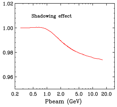
Figure 1: The ratio of photoproduction cross sections on deuterium to the sum of the photoproduction cross sections on unbound protons and neutrons. This shadowing correctionyangthesis is used to extract the photorproduction cross section on free neutrons and protons.

$$K^{LW}_{vector}(\nu) = \frac{\nu^{2}+C^{low-\nu}_{vector}}{\nu^{2}}$$

$$K_{sea-strange}^{vector}(Q^{2}) = \frac{Q^{2}}{Q^{2}+C_{sea-strange}}$$

$$K_{sea-up}^{vector}(Q^{2}) = \frac{Q^{2}}{Q^{2}+C_{sea}^{up}}$$

$$K_{sea-down}^{vector}(Q^{2}) = \frac{Q^{2}}{Q^{2}+C_{sea}^{down}}$$

$$K_{valence-up}^{vector}(Q^{2}) = K^{LW}[1-G_{D}^{2}(Q^{2})]$$

$$\times \left(\frac{Q^{2}+C_{v2u}}{Q^{2}+C_{v1u}}\right)$$

$$K_{valence-down}^{vector}(Q^{2}) = K^{LW}([1-G_{D}^{2}(Q^{2})]$$ (24)

$$\times \left(\frac{Q^{2}+C_{v2d}}{Q^{2}+C_{v1d}}\right).$$

The best fit iteration 2 parameters are $A=0.621\pm 0.009$, $B=0.380\pm 0.004$, $C_{v1d}=0.341\pm 0.007$, $C_{v1u}=0.417\pm 0.024$, $C_{v2d}=0.323\pm 0.051$, $C_{v2u}=0.264\pm 0.015$, and $C^{low-\nu}=0.218\pm 0.015$ for both down and up quarks. The sea vector parameters for iteration 2 are $C_{sea}^{down}$=0.561, $C_{sea}^{up}$=0.369, and $C_{sea}^{strange}$ is set to be the same as $C_{sea}^{down}$. Here, the parameters are in units of GeV². The factor $K^{LW}_{vector}(\nu)$ with $C^{low-\nu}_{vector}$=0.218 is needed describe the resonance region for $Q^{2}<$ 1.5 GeV² as described below

The fit yields a $\chi^{2}/DOF$ of $2357/1717$, and $N=1.026\pm 0.003$. The photo-production resonance data (above the $\Delta(1232)$) add to the $\chi^{2}/ndf$ because the fit only provides a smooth $average$ over the higher resonances. No neutrino data are included in the fit. These parameters are summarized in Table 2.

The normalization of the various experiments are allowed to float within their errors with the normalization of the SLAC proton data set to 1.0. The fit yields normalization factors of $0.986\pm 0.002$, $0.979\pm 0.003$, $0.998\pm 0.003$, $1.008\pm 0.003$, $1.001\pm 0.004$, and $0.987\pm 0.005$ for the SLAC deuterium data, BCDMS proton data, BCDMS deuterium data, NMC proton data, NMC deuterium data, and H1 proton data, respectively. With these normalization, the GRV98 PDFs with our modifications should be multiplied by N=1.026 $\pm$ 0.003.

$A$	$B$	$C_{v2d}$	$C_{v2u}$
$0.621$	$0.380$	$0.323$	$0.264$
$C_{sea}^{down}$	$C_{sea}^{up}$	$C_{v1d}$	$C_{v1u}$
$0.561$	$0.369$	$0.341$	$0.417$
$C_{sea}^{strange}$	$C^{low-\nu}_{vector}$	${\cal F}_{valence}$	$N$
$0.561$	$0.218$	$[1-G_{D}^{2}(Q^{2})]$	$1.026$

Table 2: Second iteration with GRV98 PDFs: Vector Parameters. Here, we also include photoproduction data on hydrogen and deuterium. No neutrino data are included in the fit. When applicable, all parameters are in units of GeV².

As described in section 10 we apply a small $d/u$ correction to the GRV98 PDFs. This correction increases the valence $d$ quark distribution at large $x$ and is extracted from NMC data for ${\cal F}_{2}^{D}/{\cal F}_{2}^{P}$.

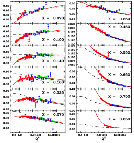
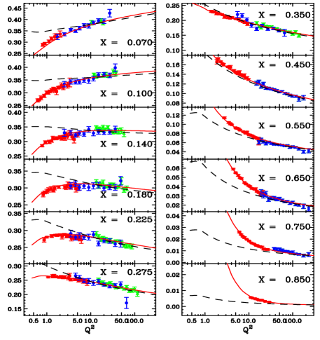
Figure 2: The effective LO PDF model (iteration 2) compared to charged-lepton ${\cal F}_{2}$ experimental data (SLAC, BCDMS, NMC) at high $x$ (these data are included in the fit) :[top] ${\cal F}_{2}$ proton, [bot] ${\cal F}_{2}$ deuteron (per nucleon). The solid lines are the fit, and the dashed lines are GRV98 .

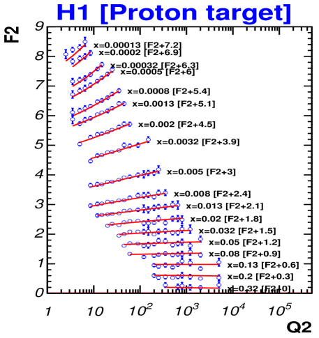
Figure 3: The effective LO PDF model (iteration 2) compared to charged-lepton ${\cal F}_{2}$ experimental data at low $x$ from H1 (these data are included in the fit).

Comparisons of the (iteration 2) fit to various sets of inelastic electron and muon ${\cal F}_{2}$ data on proton and deuteron targets are shown in Fig. 2 (for SLAC, BCDMS and NMC). Comparisons to H1(electron-proton) data at low values of $x$ are shown in Fig. 3. The effective LO model describes the inelastic charged-lepton ${\cal F}_{2}$ data both in the low $x$ as well as in the high $x$ regions. The model also provides a very good description of both low energy and high energy photoproduction cross sectionsphoto on proton and deuteron targets for incident photon energies above $\nu=0.56$ GeV (which corresponds $W>1.4$ GeV) as shown in Fig. 4.

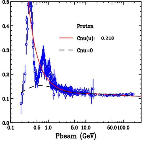
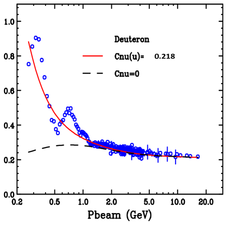
Figure 4: The effective LO PDF model (iteration 2) compared to photoproduction cross sections ($Q^{2}=0$ limit) at low and high energies (these data are included in the fit); [top] proton, [bot] deuteron (neutron plus proton). The cross sections are in units of mb. At very high photon energy, we include charm contribution from gluon fusion process which is needed to describe the very high energy HERA data. If we want to also describe the photoproduction data in the resonance region, we need to multiply the $u$ and $d$ valence PDFs by $K^{LW}=(\nu^{2}+C^{low-\nu}_{vector})/\nu^{2}$ (where $C^{low-\nu}_{vector}$=0.218). The red line includes include the $K^{LW}$ factor, and the dashed black line does not includes the $K^{LW}$ factor.

5 Comparison to resonance production data

Comparisons of the model predictionss to hydrogen and deuterium photoproduction cross sections ($Q^{2}=0$) including the resonance region are shown in Fig. 4. The corresponding electron scattering data in the resonance region jlab are shown in Fig. 5. As expected from quark-hadron duality bloom , the model provides a reasonable description of both the inelastic region as well as the $average$ value of the ${\cal F}_{2}$ data in the resonance region (down to $Q^{2}=0$), including the region of the first resonance ($W=1.23~{}GeV$). We also find good agreement with recent ${\cal F}_{L}$ and ${\cal F}_{2}$ data in the resonance region from the E94-110, and JUPITER experiments jlab ; Liang:2004tj at Jlab, as shown in Fig. 6. The predictions for ${\cal F}_{L}$ are obtained using the ${\cal F}_{2}$ model and the $R_{1998}$ R1998 parametrization (as discussed in section 7).

We find good agreement with quark hadron duality down to very low $Q^{2}$ including the region of the $\Delta$(1238) resonance. Other studiesadler2 with unmodified GRV PDFs find large deviations from quark-hadron duality in the resonance region for electron and muon scattering. This is because those studies do not include any low $Q^{2}$ $K$ factors and use the scaling variable $\xi$ (while we use the modified scaling variable $\xi_{w}$). We find that quark hadron duality works at low $Q^{2}$ if we use the modified scaling variable $\xi_{w}$, and low $Q^{2}$ $K_{i}(Q^{2})$ and $K^{LW}(\nu)$ factors.

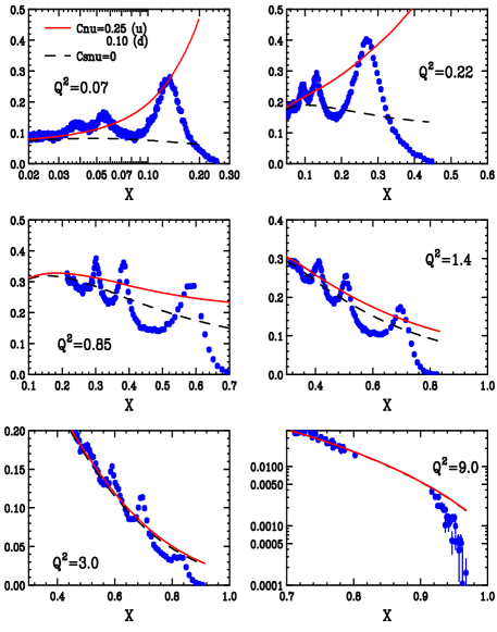
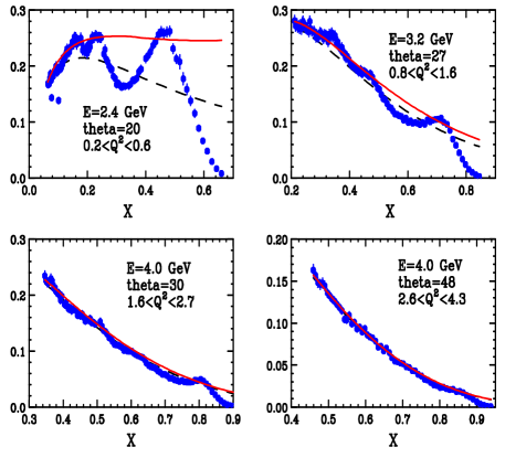
Figure 5: Comparisons of charged-lepton experimental data in the resonance region to the predictions of the iteration 2 effective LO model. The top six plots are proton ${\cal F}_{2}$ data and the bottom four plots are deuteron ${\cal F}_{2}$ data (per nucleon). The red line includes the $K^{LW}$ factor and the dashed black line does not include the $K^{LW}$ factor. Here, $K^{LW}_{vector}=(\nu^{2}+C^{low-\nu}_{vector})/\nu^{2}$ (where $C^{low-\nu}_{vector}$=0.218).

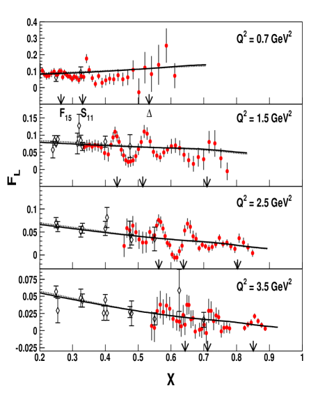
Figure 6: Comparisons of the predictions of the iteration 2 model to proton data for ${\cal F}_{L}$ (note that data for ${\cal F}_{L}$ are not included in the fit).

In the $Q^{2}=0$ photoproduction limit, the model provides a good descriptions of the data for both the inelastic region as well as the $average$ cross section in the resonance region as shown in Fig. 4.

We recommend that the model should only be used for $W>1.4$ GeV. This is because the $\Delta$(1238) resonance has isospin 3/2 and quarks have isospin of 1/2. Therefore, effective leading PDFs and quark hadron duality should NOT be valid in the region of $\Delta$(1238) resonance for neutrino scattering. Both quasielastic scattering and $\Delta$(1238) resonance production should be modeled in terms of vector and axial form factors.

6 Application to neutrino scattering

For very high energy neutrino scattering on $quarks$ and $antiquarks$ at high $Q^{2}$ , the vector and axial contributions are the same. Therefore, at high $Q^{2}$, where the naive quark parton model is valid, both the vector and axial $K$ factors are expected to be 1.0. The neutrinos and antineutrino structure functions at high $Q^{2}$ are given by :

$${\cal F}_{2}^{\nu}(x,Q^{2}) = 2\Sigma_{i}\left[\xi_{w}q_{i}(\xi_{w},Q^{2})+\xi_{w}\overline{q}_{i}(\xi_{w},Q^{2})\right].$$

and

$$x{\cal F}_{3}^{\nu}(x,Q^{2}) = 2\Sigma_{i}\left[\xi_{w}q_{i}(\xi_{w},Q^{2})-\xi_{w}\overline{q}_{i}(\xi_{w},Q^{2})\right],$$

where

$$q^{\nu p} = d+s;~{}~{}~{}~{}\bar{q}^{\nu p}=\bar{u}+\bar{c}$$

$$q^{\nu n} = u+s;~{}~{}~{}~{}\bar{q}^{\nu n}=\bar{d}+\bar{c}$$

$$q^{\bar{\nu}p} = u+c;~{}~{}~{}~{}\bar{q}^{\bar{\nu}p}=\bar{d}+\bar{s}$$

$$q^{\bar{\nu}n} = d+c;~{}~{}~{}~{}\bar{q}^{\bar{\nu}n}=\bar{u}+\bar{c}.$$ (25)

Here, ${\cal F}_{2}=\nu{\cal W}_{2}$, ${\cal F}_{1}=M{\cal W}_{1}$ and ${\cal F}_{3}=\nu{\cal W}_{3}$. Note that for the strangeness conserving $(sc)$ part of the $u$ and $d$ quark distributions, the PDFs are multiplied by a factor of $cos^{2}\theta_{c}$=0.97417(21) where $\theta_{c}$ is the Cabbibo angle. For the strangeness non-conserving part the PDFs are are multiplied by a factor of $sin^{2}\theta_{c}$=0.2248(10).

For GRV98 the charm quark distribution c=0. Noting that $d^{n}=u^{p}$, $u^{n}=d^{p}$, $\bar{d}^{n}=\bar{u}^{p}$, and $\bar{u}^{n}=\bar{d}^{p}$) we separate the distributions into non-charm production (ncp) and charm production (cp) terms.

For neutrino scattering on protons (here the items in parenthesis are explanations of the process)

$$q^{\nu p}(W^{+}ncp) = d_{v}cos^{2}\theta_{c}(d^{p}_{v}\rightarrow u)+s~{}sin^{2}\theta_{c}[s^{p}\rightarrow u)$$

$$+ d_{sea}~{}cos^{2}\theta_{c}(d^{p}_{sea}\rightarrow u)$$

$$q^{\nu p}(W^{+}{cp}) = d_{v}sin^{2}\theta_{c}(d^{p}_{v}\rightarrow c)+s~{}cos^{2}\theta_{c}[s^{p}\rightarrow c)$$

$$+ d_{sea}~{}sin^{2}\theta_{c}(d^{p}_{sea}\rightarrow c)$$

$$\bar{q}^{\nu p}(W^{+}ncp) = \bar{u}_{sea}(\bar{u}^{p}_{sea}\rightarrow[\bar{d}+\bar{s}]).$$ (26)

For neutrino scattering on neutrons (here the items in parenthesis are explanations of the process)

$$q^{\nu n}(W^{+}ncp) = u_{v}cos^{2}\theta_{c}(d^{n}_{v}\rightarrow u)+s~{}sin^{2}\theta_{c}[s^{n}\rightarrow u)$$

$$+ u_{sea}cos^{2}\theta_{c}(d^{n}_{sea}\rightarrow u)$$

$$q^{\nu n}(W^{+}{cp}) = u_{v}sin^{2}\theta_{c}(d^{n}_{sea}\rightarrow c)+s~{}cos^{2}\theta_{c}(s^{n}\rightarrow c)$$

$$+ u_{sea}~{}sin^{2}\theta_{c}(d^{n}_{sea}\rightarrow c)$$

$$\bar{q}^{\nu p}(W^{+}ncp) = \bar{d}_{sea}(\bar{u}^{n}_{sea}\rightarrow[\bar{d}+\bar{s}]).$$ (27)

For antineutrino scattering on protons

$$\bar{q}^{\bar{\nu}p}(W^{-}ncp) = \bar{d}_{sea}cos^{2}\theta_{c}(\bar{d}^{p}_{sea}\rightarrow\bar{u})+\bar{s}~{}sin^{2}\theta_{c}(\bar{s}^{p}\rightarrow\bar{u})$$

$$\bar{q}^{\bar{\nu}p}(W^{-}{cp}) = \bar{d}_{sea}sin^{2}\theta_{c}(\bar{d}^{p}_{ses}\rightarrow\bar{c})+\bar{s}~{}cos^{2}\theta_{c}(\bar{s}^{p}\rightarrow\bar{c})$$

$$q^{\bar{\nu}p}(W^{-}ncp) = u_{v}(u^{p}_{v}\rightarrow[d+s])$$ (28)

$$+ u_{sea}(u^{p}_{sea}\rightarrow[d+s])$$

For antineutrino scattering on neutrons

$$\bar{q}^{\bar{\nu}n}(W^{-}ncp) = \bar{u}_{sea}cos^{2}\theta_{c}(\bar{d}^{n}_{sea}\rightarrow\bar{u})+\bar{s}~{}sin^{2}\theta_{c}(\bar{s}^{n}\rightarrow\bar{u})$$

$$\bar{q}^{\bar{\nu}n}(W^{-}cp) = \bar{u}_{sea}sin^{2}\theta_{c}(\bar{d}^{n}_{sea}\rightarrow\bar{c})+\bar{s}~{}cos^{2}\theta_{c}(\bar{s}^{n}\rightarrow\bar{c})$$

$$q^{\bar{\nu}n}(W^{-}ncp) = d_{v}(u^{n}_{v}\rightarrow[d+s])$$ (29)

$$+ d_{sea}(u^{n}_{sea}\rightarrow[d+s])$$

There are several major difference between the case of charged-lepton inelastic scattering and the case of neutrino scattering. In the neutrino case we have one additional structure functions ${\cal F}_{3}^{\nu}(x,Q^{2})$. In addition, at low $Q^{2}$ there could be a difference between the vector and axial $K_{i}$ factors due a difference in the non-perturbative axial vector contributions. Unlike the vector ${\cal F}_{2}$ which must go to zero in the $Q^{2}=0$ limit, we expect DL ; kulagin that the axial part of ${\cal F}_{2}$ can be non-zero in the $Q^{2}=0$ limit. At $Q^{2}=0$, this non-zero axial contribution is purely longitudinal. This can be illustrated as follows. The neutrino structure functions must satisfy the following inequalities:

$$0 \leq \sqrt{1+\frac{Q^{2}}{\nu^{2}}}x{|{\cal F}_{3}|}\leq 2x{\cal F}_{1}\leq(1+\frac{Q^{2}}{\nu^{2}}){\cal F}_{2},$$

which indicates that only ${\cal F}_{2}$ can be non zero at $Q^{2}=0$.

We already account for kinematic, dynamic higher twist and higher order QCD effects in ${\cal F}_{2}$ by fitting the parameters of the scaling variable $\xi_{w}$ (and the $K$ factors) to low $Q^{2}$ data for ${\cal F}_{2}^{e\mu}(x,Q^{2})$. These should also be valid for the vector part of ${\cal F}_{2}$ in neutrino scattering.

$${\cal F}_{2}^{\nu,vector}(x,Q^{2})=\Sigma_{i}K_{i}^{vector}(Q^{2})\xi_{w}q_{i}(\xi_{w},Q^{2})$$

$$+\Sigma_{j}K_{j}^{vector}(Q^{2})\xi_{w}\overline{q}_{j}(\xi_{w},Q^{2}).$$ (30)

However, the higher order QCD effects in ${\cal F}_{2}$ and $x{\cal F}_{3}$ are different. We account for the different scaling violations in ${\cal F}_{2}$ and $x{\cal F}_{3}$ (from higher order QCD terms) by adding a correction factor $H(x,Q^{2})$ as follows.

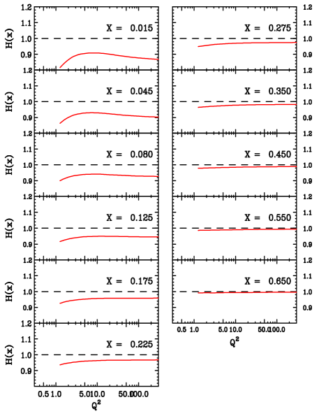
Figure 7: The $x$ and $Q^{2}$ dependence of the factor $H(x,Q^{2})$ that accounts for the difference in the QCD higher order corrections in ${\cal F}_{2}$ and $x{\cal F}_{3}$

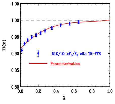
Figure 8: A fit to the $x$ dependence of the factor $H(x,Q^{2})$ that accounts for the difference in the QCD higher order corrections in ${\cal F}_{2}$ and $x{\cal F}_{3}$ (at $Q^{2}=8~{}GeV^{2})$.

$$x{\cal F}_{3}^{\nu}(x,Q^{2})=2H(x,Q^{2})\Biggl{\{}\Sigma_{i}K^{vector}_{i}\xi_{w}q_{i}(\xi_{w},Q^{2})$$

$$-\Sigma_{j}K^{vector}_{j}\xi_{w}\overline{q}_{j}(\xi_{w},Q^{2})\Biggr{\}}.$$ (31)

We obtain an approximate expression for $H(x,Q^{2})$ as the ratio of two ratios as follows:

$$H(x,Q^{2})=D_{x{\cal F}_{3}}(x,Q^{2})/D_{{\cal F}_{2}}(x,Q^{2}),$$ (32)

where

$$D_{xF3}(x,Q^{2}) = \frac{x{\cal F}_{3}^{nlo}(x,Q^{2})}{x{\cal F}_{3}^{lo}(x,Q^{2})}$$

$$D_{F2}(x,Q^{2}) = \frac{{\cal F}_{2}^{nlo}(x,Q^{2})}{{\cal F}_{2}^{lo}(x,Q^{2})}.$$ (33)

The double ratio $H(x,Q^{2})$ is calculated by the TR-VFS schemexf3calc with MRST991 NLO PDFs. This ratio turns out to be almost independent of $Q^{2}$. The results of this calculation at $Q^{2}=8$ GeV², shown in Fig. 8 are fitted with the following functional form:

$$H(x,Q^{2}) = 0.914+0.296x-0.374x^{2}+0.165x^{3}.$$ (34)

We use the above approximation for $H(x,Q^{2})$ for all values of $Q^{2}$.

In our previous nuint01-2 analysis we assumed $H(x,Q^{2})$=1, and $K_{i}^{axial}(Q^{2})$= $K_{i}^{vector}(Q^{2})$. This assumption is only valid for at high $Q^{2}$ ($Q^{2}>1~{}GeV^{2}$). Here, we improve on the previous analysis by introducing $K_{i}^{axial}(Q^{2})$ factors which are different from $K_{i}^{vector}(Q^{2})$, and include the $H(x,Q^{2})$ correction for $x{\cal F}_{3}$.

7 $2x{\cal F}_{1}$ and the longitudinal structure function

In the extraction of the original GRV98 LO PDFs, no separate longitudinal contribution was included. The quark distributions were directly fit to ${\cal F}_{2}$ data. A full modeling of electron and muon cross section requires also a description of $2x{\cal F}_{1}$. In general, $2x{\cal F}_{1}^{e/\mu}$ and ${\cal W}_{1}^{e/\mu}$ are given in terms of ${\cal F}_{2}$ and ${\cal R}$ in equation 12. For the vector contribution we use a non-zero longitudinal ${\cal R}$ in reconstructing $2x{\cal F}_{1}$ by using a fit of ${\cal R}$ to measured data. The ${\cal R}_{1998}$ functionR1998 provides a good description of the world’s data for ${\cal R}$ in the $Q^{2}>0.3$ GeV² and $x>0.05$ region (where most of the ${\cal R}$ data are available).

$${\cal R}_{e/\mu}(x,Q^{2}>0.3) = {\cal R}_{1998}(x,Q^{2}>0.3)$$

However, the ${\cal R}_{1998}$ function breaks down at low $Q^{2}$. Therefore, we freeze the function at $Q^{2}=0.3$ GeV² and introduce a $K$ factor for ${\cal R}$ in the $Q^{2}<0.3$ GeV² region to make a smooth transition for ${\cal R}_{e/\mu}$ from $Q^{2}=0.3$ GeV² down to $Q^{2}=0$ by forcing ${\cal R}_{vector}$ to approach zero at $Q^{2}=0$, as expected in the photoproduction limit. This procedure keeps a $1/Q^{2}$ behavior at large $Q^{2}$ and matches to ${\cal R}_{1998}$ at $Q^{2}=0.3$ GeV²,

$${\cal R}_{e/\mu}(x,Q^{2}<0.3) = 3.633\frac{Q^{2}}{Q^{4}+1}\times{\cal R}_{1998}(x,Q^{2}=0.3).$$

Using the above fits to ${\cal R}$ as measured in electron/muon scattering we use the following expressions for the vector part of $2x{\cal F}_{1}$ neutrino scattering:

$$2x{\cal F}_{1}^{vector}(x,Q^{2}) = {\cal F}_{2}^{vector}(x,Q^{2})\frac{1+4M^{2}x^{2}/Q^{2}}{1+{\cal R}(x,Q^{2})}$$

$${\cal R}_{vector}(x,Q^{2}>0.3) = {\cal R}_{1998}(x,Q^{2}>0.3)$$

$${\cal R}_{vector}(x,Q^{2}<0.3) = {\cal R}_{e/\mu}(x,Q^{2}<0.3).$$

The above expressions have the correct limit for the vector contribution at $Q^{2}=0$.

A recent fit to ${\cal R}$ that includes updated ${\cal R}$ measurements from Jefferson Lab (including resonance data) has been published by M.E. Christy and P.E. BostedjlabR . In the kinematic region of the fits the difference between the Christy-Bosted fit and the ${\cal R}_{1998}$ fit is small.

7.1 Nuclear Corrections to R

In the analysis we use the ${\cal R}_{1998}$ parametrization. Preliminary results from the JUPITER Jefferson Lab collaboration indicates that ${\cal R}$ for heavy nucleus may be higher by about 0.1 than $R$ for deuterium. Therefore, we use an error of $\pm$0.1 in R to estimate the systematic error in the cross sections from this source.

8 Charm production in neutrino scattering

Neutrino scattering is not as simple as the case of charged-lepton scattering because of the contribution from charm production (cp). For non-charm production (ncp) components we use the sum of the vector and axial contributions to ${\cal F}_{2}^{ncp}(x,Q^{2})$, and $2x{\cal F}_{1}^{ncp}(x,Q^{2}$) with $x{\cal F}_{3}^{ncp}(x,Q^{2})$ as described above.

For the charm production components of ${\cal F}_{2}^{cp}(x,Q^{2})$, $x{\cal F}_{3}^{cp}(x,Q^{2})$ and $2x{\cal F}_{1}^{cp}(x,Q^{2})$ the variable $\xi_{w}$ is replaced with $\xi_{w}^{\prime}$ includes a non-zero final state quark mass $M_{c}=1.32~{}GeV$.

$$\xi_{w}^{\prime} = \frac{Q^{2}+1.32^{2}+B}{M\nu[1+\sqrt{1+Q^{2}/\nu^{2}}]+A},$$ (35)

The target mass calculations as discussed by Barbieri et. albarb imply that ${\cal F}_{2}^{\nu-cp}$ is described by ${\cal F}_{2}^{\nu-cp}(\xi_{w}^{\prime},Q^{2})$, and the other two structure functions are multiplied by the factor $K_{charm}=\frac{Q^{2}}{Q^{2}+M_{C}^{2}}$. Consequently, we use the following expression for charm production processes:

$${\cal F}_{2}^{\nu,vector-cp}(x,Q^{2})=\Sigma_{i}K_{i}^{vector}(Q^{2})$$

$$\times\left[\xi_{w}^{\prime}q_{i}(\xi_{w}^{\prime},Q^{2})+\xi_{w}^{\prime}\overline{q}_{i}(\xi_{w}^{\prime},Q^{2})\right],$$

$$2x{\cal F}_{1}^{\nu,vector-cp}(x.Q^{2}) = K_{charm}$$

$$\times \frac{1+4M^{2}x^{2}/Q^{2}}{1+{\cal R}(\xi_{w}^{\prime},Q^{2})}{\cal F}_{2}^{\nu,vector-cp}(x,Q^{2}),$$

$$K_{charm} = \frac{Q^{2}}{Q^{2}+M_{C}^{2}},$$

and

$$x{\cal F}_{3}^{\nu,cp}(x,Q^{2})=2H(x,Q^{2})K_{charm}\times$$

$$\Biggl{\{}\Sigma_{i}K^{vector}_{i}\xi_{w}^{\prime}q_{i}(\xi_{w}^{\prime},Q^{2})-\Sigma_{j}K^{vector}_{j}\xi_{w}^{\prime}\overline{q}_{j}(\xi_{w}^{\prime},Q^{2})\Biggr{\}}.$$

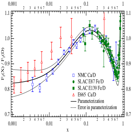
Figure 9: The ratio of ${\cal F}_{2}$ data for heavy nuclear targets and deuterium as measured in charged-lepton scattering experiments(SLAC,NMC, E665). The band show the uncertainty of the parametrized curve (as a function of $x$) from the statistical and systematic errors in the experimental data selthesis .We do not use this fit in our analysis. Instead we use another fit that includes only SLAC and Jefferson Lab data.

We use the ${\cal R}_{1998}$ parametrization R1998 for the vector part of ${\cal R}^{ncp}$ and ${\cal R}^{cp}$. Because of the suppression of charm production at low $Q^{2}$ we assume that the vector and axial contributions to charm production are equal.

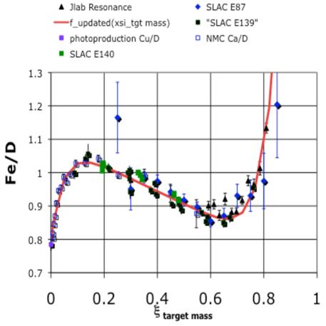
Figure 10: A a comparison of Jefferson lab measurements of the ratio of electron scattering cross sections on an isoscalar iron target to deuterium in the resonance regionarrington to data from SLAC E87e87 , SLAC E139e139 , SLAC E140e140 and NMCNMCnuc in the deep inelastic region. The data plotted versus $\xi_{TM}$ are compared to the updated fit function $f_{updated}^{Fe/D}(\xi_{TM})$. For comparison we also show the ratio as measured in photoproductionphoto at $\xi_{TM}=0$. We use this fit to cross section ratios in our analysis.

9 Nuclear corrections

In the comparison with neutrino charged-current differential cross section on an isoscalar iron target, a nuclear correction for iron targets should be applied. Previously, we used the following parameterized function, $f^{Fe/D}(x)$ (a fit to experimental electron and muon scattering data for the ratio of isoscalar iron to deuterium cross sections, shown in Fig. 9), to convert deuterium structure functions to (isoscalar) iron structure functions selthesis ;

$$f^{Fe/D}(x) = \frac{{\cal}F_{2}^{Fe}}{{\cal F}_{2}^{D}}=1.096-0.364~{}x$$ (36)

$$- 0.278~{}e^{-21.94~{}x}+2.772~{}x^{14.417}.$$

However, in this publication we do not use the above nuclear corrections for iron since they are a function of $x$ and include very high $Q^{2}$ data. We find that the ratio of iron to deuterium structure function measurements at SLAC and Jefferson Lab are better described in terms of the target mass (or Nachtman) variable $\xi_{TM}$. If $\xi_{TM}$ is used, then the function that describes the iron to deuterium ratios in the deep inelastic region is also valid in the resonance region. In addition, since we are interested primarily in low energy neutrino cross sections we only include SLAC and Jefferson lab data in our fit. We use the following updated function $f_{updated}^{Fe/D}(\xi_{TM})$.

$$f_{updated}^{Fe/D}(\xi_{TM}) = \frac{{\cal}F_{2}^{Fe}}{{\cal F}_{2}^{D}}=1.096-0.38~{}\xi_{TM}$$ (37)

$$- 0.3~{}e^{-23\xi_{TM}}+8~{}\xi_{TM}^{15}.$$

Fig. 10 shows a comparison of Jefferson lab measurements of the ratio of electron scattering cross sections on iron to deuterium in the resonance regionarrington to data from SLAC E87e87 , SLAC E139e139 , SLAC E140e140 and NMCNMCnuc in the deep inelastic region. The data plotted versus $\xi_{TM}$ are compared to the updated fit ${\cal F}_{updated}(\xi_{TM})$. For comparison we also show the ratios as measured in photoproductionphoto at $\xi_{TM}=0$.

For the ratio of deuterium cross sections to cross sections on free nucleons we use the following function obtained from a fit to SLAC data on the nuclear dependence of electron scattering cross sections yangthesis .

$$f^{D/(n+p)}(x) = 0.985\times(1+0.422x-2.745x^{2}$$ (38)

$$+ 7.570x^{3}-10.335x^{4}+5.422x^{5}).$$

This correction shown in Fig. 11 is only valid in the $0.05<x<0.75$ region.

Figures 12 show the measured ratio of structure functions for gold (Au)e140 or lead (Pb)NMCnuc to the structure functions for iron (Fe) versus $\xi_{TM}$. Fig. 13 shows the ratio of the structure functions for iron to the structure functions for carbon versus $\xi_{TM}$.

The gold (and lead) data are described by the function

$$\frac{{\cal F}_{2}^{Au,Pb}}{{\cal F}_{2}^{Fe}}(\xi_{TM})=0.932+2.461\xi-24.23\xi_{TM}^{2}$$

$$+ 101.03\xi_{TM}^{3}-203.47~{}\xi_{TM}^{4}+193.85~{}\xi_{TM}^{5}-69.82~{}\xi_{TM}^{6}.$$

The carbon datae140 ; jlabC are described by the function

$$\frac{{\cal}F_{2}^{Fe}}{{\cal F}_{2}^{C}}(\xi_{TM}) = 0.919+1.844\xi_{TM}-12.73\xi_{TM}^{2}$$ (40)

$$+ 36.89\xi_{TM}^{3}-46.77\xi_{TM}^{4}+21.22\xi_{TM}^{5}.$$

All of these ratios are for structure functions which have been corrected for the neutron excess in the nucleus and therefore account for nuclear effects only.

In neutrino scattering, we assume that the nuclear correction factors for ${\cal F}_{2}$, $x{\cal F}_{3}$ and $2x{\cal F}_{1}$ are the same. This is a source of systematic error because the nuclear shadowing corrections at low $x$ can be different for the vector and axial structure functions. This difference can be accounted for by assuming a specific theoretical modelkulagin .

9.1 Avoiding double counting of Fermi motion

Note that when the model implemented in neutrino Monte Carlo generators we must be careful not to double count the effect of Fermi motion. The above fits include the effect of Fermi motion at high $\xi_{TM}$. If Fermi motion is applied to the structure functions, than it is better to assume that the ratio of iron to deuterium without Fermi motion for $\xi_{TM}>0.65$ is equal to the ratio at $\xi_{TM}=0.65$.

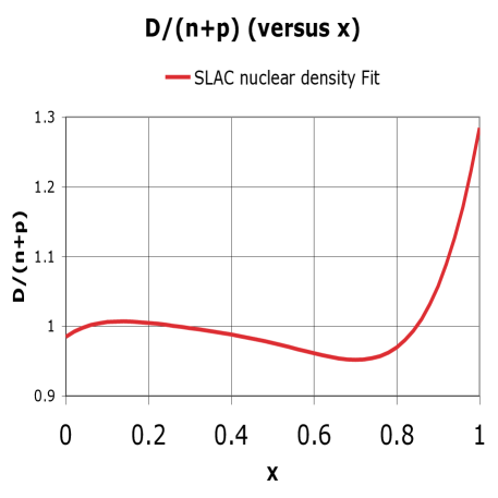
Figure 11: The total correction for nuclear effects (binding and Fermi motion) in the deuteron, $f^{D/(n+p)}(x)={\cal F}_{2}^{d}/{\cal F}_{2}^{n+p}$, as a function of $x$, extracted from fits to the nuclear dependence of SLAC ${\cal F}_{2}$ electron scattering data. This correction is only valid for $0.05<x<0.75$.

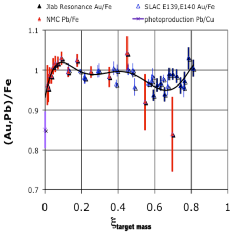
Figure 12: The ratio of ${\cal F}_{2}$ data for gold (Au) to ${\cal F}_{2}$ data for Iron (Fe) as measured in charged-lepton scattering experiments in the deep inelastic region (SLAC E139, SLAC E140) as compared to Jlab data in the resonance region versus the target mass (or Nachtman) variable $\xi_{TM}$. Also shown is the ratio of ${\cal F}_{2}$ data for lead (Pb) to ${\cal F}_{2}$ data for iron (Fe) from the NMCNMCnuc collaboration. For comparison we also show the ratio of lead to copper cross sections (Pb/Cu) as measured in photoproductionphoto .

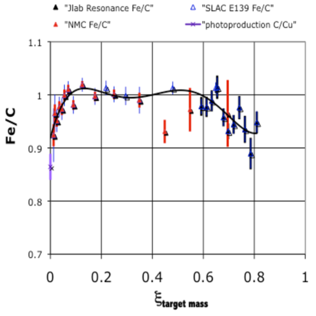
Figure 13: The ratio of ${\cal F}_{2}$ data for iron (Fe) to ${\cal F}_{2}$ data for carbon (C) to as measured in charged-lepton scattering in the deep inelastic region (SLAC E139) as compared to Jlab data in the resonance region versus the target mass, or Nachtman variableNachtman $\xi_{TM}$. Also shown is the ratio of ${\cal F}_{2}$ data for carbon to ${\cal F}_{2}$ data for iron from the NMCNMCnuc collaboration. For comparison we also show the ratio of of carbon to copper cross sections (C/cu) as measured in photoproductionphoto .

10 d/u correction

The $d/u$ correction for the GRV98 LO PDFs is obtained from the NMC data for ${\cal F}_{2}^{D}/{\cal F}_{2}^{P}$. Here, Eq. 38 is used to remove nuclear binding effects in the NMC deuterium ${\cal F}_{2}$ data. The correction term, $\delta(d/u)$ is obtained by keeping the total valence and sea quarks the same.

$$\delta(d/u)(x)=-0.00817+0.0506x+0.0798x^{2},$$ (41)

where the corrected $d/u$ ratio is $(d/u)^{\prime}=(d/u)+\delta(d/u)$. Thus, the modified $u$ and $d$ valence distributions are given by

$$u_{v}^{\prime}=\frac{u_{v}}{1+\delta(d/u)\frac{u_{v}}{u_{v}+d_{v}}}$$ (42)

$$d_{v}^{\prime}=\frac{d_{v}+u_{v}\delta(d/u)}{1+\delta(d/u)\frac{u_{v}}{u_{v}+d_{v}}}.$$ (43)

The same formalism is applied to the modified $u$ and $d$ sea distributions. We find that the modified $u$ and $d$ sea distributions (based on NMC data) also agree with the NUSEA data in the range of $x$ between 0.1 and 0.4. Thus, we find that corrections to $u$ and $d$ sea distributions are not necessary.

11 Axial structure functions ${\cal F}_{2}$, and $2x{\cal F}_{1}$

At $Q^{2}=0$ the vector structure function ${\cal F}_{2}^{\nu-vector}$ is required to go to zero. In contrast, the axial structure function ${\cal F}_{2}^{\nu-axial}$ is not constrained to go to zero at $Q^{2}=0$. At higher $Q^{2}$ ($>$1.5 GeV²) the vector and axial structure functions should be equal. Since the contribution of the structure function $2x{\cal F}_{1}$ to the cross section near $Q^{2}=0$ is very small we set

$${2x\cal F}_{1}^{\nu-axial}(x,Q^{2}) = {2x\cal F}_{1}^{\nu-vector}(x,Q^{2}).$$ (44)

The axial contribution at small $Q^{2}$ is primarily longitudinal and only contributes to ${\cal F}_{2}$.

We compare neutrino data to two versions of the model as shown below.

11.1 Effective LO PDFs Model Type I (axial=vector)

The first version of the model (which we refer to as Type I(A=V)) assumes that the vector and axial components of the structure function ${\cal F}_{2}^{\nu}$ are equal at all values of $Q^{2}$. i.e.

$${\cal F}_{2}^{\nu-axial}(x,Q^{2})={\cal F}_{2}^{\nu-vector}(x,Q^{2})~{}(Type~{}I).$$ (45)

This is the assumption that has been made in previous implementations of our model. This assumption underestimates the neutrino cross section at low $Q^{2}$. In contrast, the assumption that the K axial factors are 1.0 overestimates the cross section. To properly model neutrino interactions propose the Type II (A$>$V) model described below.

11.2 Effective LO PDFs model Type II (A$>$V) (a better model)

In this version of the model we account for the fact that the axial and vector structure functions are not equal at $Q^{2}$=0 as follows:

$${\cal F}_{2}^{\nu-axial}(x,Q^{2})=\Sigma_{i}K_{i}^{axial}(Q^{2})\xi_{w}q_{i}(\xi_{w},Q^{2})$$

$$+\Sigma_{j}K_{j}^{axial}(Q^{2})\xi_{w}\overline{q}_{j}(\xi_{w},Q^{2}).$$ (46)

11.2.1 Axial sea

For sea quarks, use use the same axial $K$ factor for all types of quarks.

$$K_{sea}^{axial}(Q^{2}) = \frac{Q^{2}+P_{sea}^{axial}C_{sea}^{axial}}{Q^{2}+C_{sea}^{axial}}$$

where $P_{sea}^{axial}=0.55\pm 0.05$, and $C_{sea}^{axial}=0.75\pm 0.25$ yielding

$$K_{sea}^{axial}(Q^{2}) = \frac{Q^{2}+0.41}{Q^{2}+0.75}~{}(Type~{}II).$$ (47)

We use 30% of the difference between the cross section predictions of the Type I (A=V) and Type II (A$>$V) models as an estimate of the uncertainty in the axial $K$ factors.

11.2.2 Explanation of the origin of the axial sea

We refer to the non-zero value of the $K_{sea}^{axial}$ at $Q^{2}$=0 as the PCAC term in ${\cal F}_{2}$. We obtain the parameters $P_{sea}^{axial}=0.55\pm 0.05$, and $C_{sea}^{axial}=0.75\pm 0.25$ using the following relation,

$${\cal F}_{2}^{axial-sea}={\cal F}_{2}^{vector-sea}+{\cal F}_{2}^{PCAC}$$ (48)

where ${\cal F}_{2}^{PCAC}$ is from the model of Kulagin and Petikulagin .

As a check, we note that the CCFRbonnie collaboration has reported on a measurement (via an extrapolation) of ${\cal F}_{2}^{Fe}$ at $Q^{2}=0$. The CCFR value for an iron target (per nucleon) ${\cal F}_{2}^{Fe}(Q^{2}=0)$=0.210$\pm$0.02, is in agreement with our model prediction for ${\cal F}_{2}^{axial,Fe}(x=10^{-5},Q^{2}=0)$=0.251$\pm$0.025. Our value is obtained using $P_{sea}^{axial}=0.55\pm 0.05$ in conjunction with ${\cal F}_{2}^{GRV98}$=0.57 for $Q^{2}=0.8$ GeV² and $x=10^{-5}$ (assuming a nuclear shadowing ratio ${\cal F}_{2}^{Fe}/{\cal F}_{2}^{D}=0.8$.)

11.2.3 Axial valence

For the valence quarks, we note that the following is a good approximation to the vector $K$ factor.

$$K^{vector}_{valence}(Q^{2})\approx[1-G_{D}^{2}(Q^{2})]\approx\frac{Q^{2}}{Q^{2}+0.18}.$$ (49)

Where $Q^{2}$ is in units of GeV². We use a similar form for the axial $K$ factor for valence quarks.

$$K^{axial}_{valence}(Q^{2})=\frac{Q^{2}+P_{valence}^{axial}\times 0.18}{Q^{2}+0.18}~{}(Type~{}II).$$ (50)

Where $P_{valence}^{axial}=0.3$ is chosen to get better agreement with measured high energy neutrino and antineutrino total cross sections. In summary,

$$K^{axial}_{valence}(Q^{2})=\frac{Q^{2}+0.054\pm 0.009}{Q^{2}+0.18}~{}(Type~{}II),$$ (51)

which implies that the axial $K$ factor for the valence quarks at $Q^{2}=0$ is 0.3. We use the same axial $K$ factor for the $u$ and $d$ valence quarks. As mentioned earlier, we assume $2x{\cal F}_{1}^{axial}=2x{\cal F}_{1}^{vector}$. This is because the non-zero PCAC component of ${\cal F}_{2}^{axial}$ at low $Q^{2}$ is purely longitudinal and therefore does not contribute to $2x{\cal F}_{1}^{axial}$ which is purely transverse.

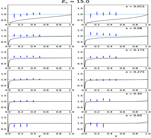
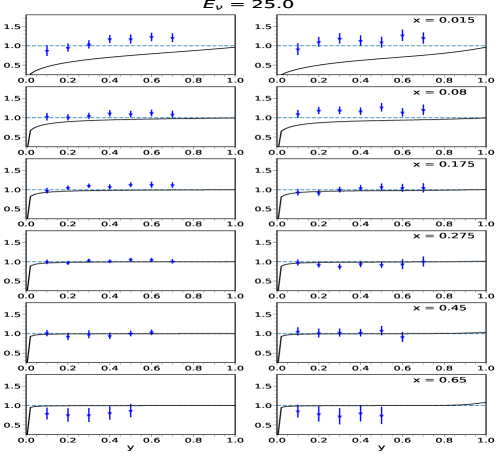
Figure 14: Same as Fig.15 for energies of 15 and 25 $GeV$ (CCFR data only).

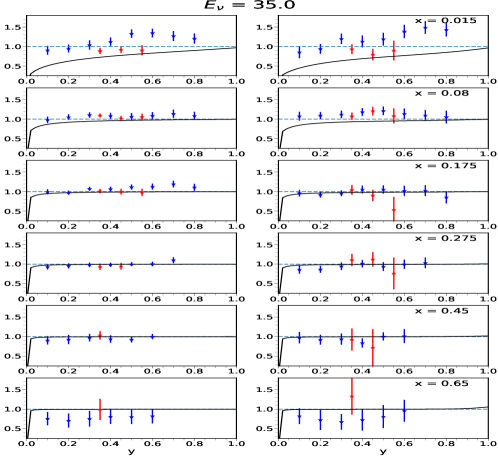
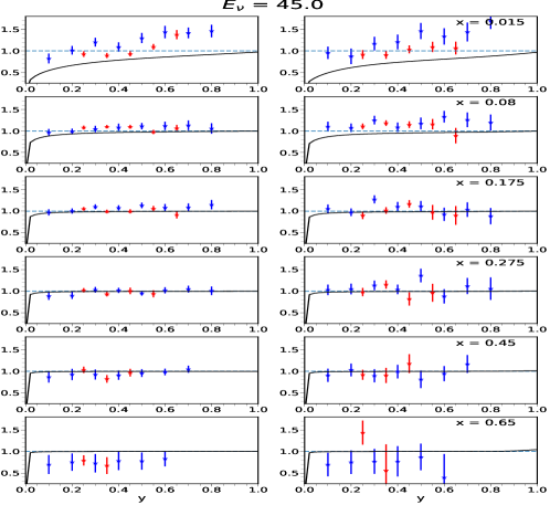
Figure 15: The ratio of charged-current neutrino and antineutrino differential cross sections $d^{2}\sigma/dxdy$ on lead from CHORUS chorus (blue points) and CCFR cross sections (red points) on iron yangthesis ; rccfr to Type II (A$>$V) default model. The ratios are shown for energies of 35 and 45 $GeV$. On the left side we show the comparison for neutrino cross sections and on the right side we show the comparsons for antineutrinos. The black line is the ratio of the predictions of the Type I (A=V) model for which the axial structure functions are set equal to the vector structure functions, to the predictions of the Type II (A$>$V) default model. The CHORUS and CCFR data favor the Type II (A$>$V) model.

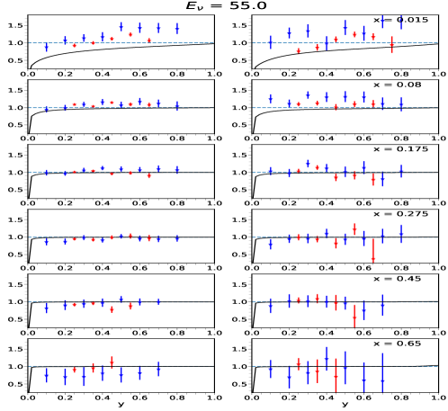
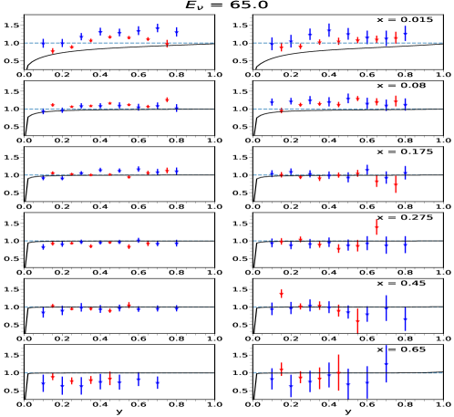
Figure 16: Same as Fig.15 for energies of 55 and 65 $GeV$.

12 Comparison to inelastic $\nu$ and $\overline{\nu}$ cross sections on nuclear targets

12.1 $\nu$ and $\overline{\nu}$ differential cross section data

We compare the model predictions to neutrino differential cross sections ($\frac{d^{2}\sigma^{\nu(\overline{\nu})}}{dxdy}$) on lead (CHORUS chorus ) and iron (CCFR yangthesis ; rccfr ). We multiply the CHORUS cross sections by ratio of the nuclear corrections for iron divided by the nuclear correction for lead, such that both differential cross sections can be shown on the same plot and compare to the predictions for the neutrino differential cross sections on iron. The neutrino (antineutrino) differential cross section is given by:

$$\frac{d^{2}\sigma^{\nu(\overline{\nu})}}{dxdy} = \frac{G_{F}^{2}ME}{\pi}{\Big{(}}\Big{[}1-y(1+\frac{Mx}{2E})\Big{]}{\cal F}_{2}+\frac{y^{2}}{2}(2x{\cal F}_{1})$$ (52)

$$\pm \Big{[}y-\frac{y^{2}}{2}\Big{]}x{\cal F}_{3}{\Big{)}}.$$

where ${\cal F}_{2}={\cal F}_{2}^{vector}+{\cal F}_{2}^{axial}$, ${\cal F}_{1}={\cal F}_{1}^{vector}+{\cal F}_{1}^{axial}$, and $G_{F}/(\hbar c)^{3}=1.1663787(6)\times 10^{-5}$ GeV^-2 is the Fermi coupling constant and $(\hbar c)^{2}$= 0.389 379 3656(48) GeV² mbarn.

In the comparison we assume that the ratio of neutrino structure functions for nucleons bound in a nucleus to neutrino structure functions free nucleons for neutrinos is equal to the ratio measured in electron/muon scattering for ${\cal F}_{2}$. We also assume that the nuclear corrections are the same for the axial and vector part of the structure functions. This is a source of systematic error because the nuclear shadowing corrections at low $x$ can be different for the vector and axial terms (this difference can be accounted for by assuming a specific theoretical modelkulagin ).

The published CHORUS and CCFR differential cross sections have been corrected for radiative corrections. In addition, the CHORUS and CCFR data are corrected for the neutron excess in lead and iron. Consequently, we compare the CHORUS data to the model prediction for isoscalar (i.e. equal number of neutrons and protons) lead and iron targets .

Figures 14-16 show the ratio of charged-current neutrino and antineutrino differential cross sections $d^{2}\sigma/dxdy$ on lead from CHORUS (blue points) and CCFR cross sections on iron (red points), to the Type II (A$>$V) default model. The ratios are shown for neutrino energies of 15, 25, 35, 45, 55 and 65 $GeV.$ On the left side we show the comparison for neutrinos and on the right side we show the comparison for antineutrinos. The black line is the ratio of the predictions of the Type I (A=V) model for which the axial structure functions are set equal to the vector structure functions, to the predictions of the Type II (A$>$V) default model. The CHORUS and CCFR data favor the Type II (A$>$V) model.

$P_{sea}^{axial}$	$C_{sea}^{axial}$	$P_{sea}^{valence}$
$0.55$	$0.75$	$0.3$
$C^{low-\nu(\nu)}_{axial}$	$C^{low-\nu(\overline{\nu})}_{axial}$
$0.436$	$0.654$

Table 3: A summary of the axial parameters for the Type II (A$>$V) default model. All parameters are in units of GeV².

12.2 Modeling $\nu$ and $\overline{\nu}$ cross sections in the resonance region

As mentioned earlier, the $K^{LW}_{vector}$ factor should be included for a better description of electron scattering and photo-production $average$ cross sections in in the resonance region. For the vector structure functions $K^{LW}_{vector}=(\nu^{2}+C^{low-\nu}_{vector})/\nu^{2}$ (where $C^{low-\nu}_{vector}$=0.218 GeV² ) as shown in equation 4.

In order to better describe the low energy neutrino and antineutrino total cross sections (as discussed below) we find that the $K^{LW}$ factor for the $axial$ part of the cross section in the resonance region is larger and is different for neutrinos and antineutrinos,

$$K^{LW-(\nu,\overline{\nu})}_{axial}=\frac{\nu^{2}+C_{axial}^{low-\nu(\nu,\overline{\nu})}}{\nu^{2}}$$

For neutrinos:

$$C^{low-\nu(\nu)}_{axial}=0.436~{}GeV^{2}$$

For antineutrinos

$$C^{low-\nu(\overline{\nu})}_{axial}=0.654~{}GeV^{2}.$$

A summary of the axial parameters is given in Table 3.

12.3 Comparisons to $\nu$ and $\overline{\nu}$  total cross section measurements for $E_{\nu}>30$ GeV

To test the validity of the model we compare the model predictions for the $\nu$ and $\overline{\nu}$ total cross sections to measurements. In the calculation of the neutrino total cross sections includes the following components.

1. The contributions of the quasielastic (QE) cross section and the cross section for the $\Delta$($W<1.4~{}GeV$) resonance region are extracted from measurements as described in section 16.

2. The contribution of the higher resonances $1.4<W<1.8~{}GeV$ is calculated using our model.

3. The contribution of the inelastic $W>1.8$ GeV continuum is calculated using our model.

$E_{\nu}$	$QE$	$W<1.4$	$1.4<W<1.8$	$W>1.8$
GeV		GeV	GeV	GeV
		$\Delta$(1238)	resonances	inelastic
3	23.8%	19.7%	31.3%	25.2%
5	16.2%	12.5%	22.2%	48.1%
10	7.2%	6.5%	13.4%	72.8%
40	1.5%	1.6%	6.5%	90.4%
$E_{\overline{\nu}}$	$QE$	$W<1.4$	$1.4<W<1.8$	$W>1.8$
GeV		GeV	GeV	GeV
		$\Delta$(1238)	resonances	inelastic
3	40.7%	27.1%	25.6%	6.6%
5	27.8%	20.8%	33.5%	17.9%
10	15.0%	11.7%	25.2%	48.1%
40	3.1%	3.4%	7.1%	86.4%

Table 4: Percent contributions to the total cross section of QE, $\Delta(W<1.4)$ GeV, higher resonances $1.4<W<1.8$ GeV and inelastic continuum $W>1.8$ GeV.

Table 5: Model predictions for $\sigma_{\nu}$/E per nucleon (for nucleons bound in an isoscalar iron target) in units of $10^{-38}~{}cm^{2}/GeV$, $\sigma_{\bar{\nu}}$/E per nucleon in units of $10^{-38}~{}cm^{2}/GeV$, and the ratio $\sigma_{\bar{\nu}}$/$\sigma_{\nu}$ for an average neutrino energy of 40 GeV. The predictions for both the Type I (A=V) and the Type II (A$>$V) default models are compared to the averages MINOS2 of all of the world’s data for energies between 30 and 50 GeV. The axial parameters for the Type II (A$>$V) model were tuned to agree with data.

	Type I (A=V)	Type II (A$>$V)	World Average
$\sigma_{\nu}$ /E	0.656 $\pm$0.024	0.674 $\pm$0.024	0.675 $\pm$0.006
${\sigma_{\bar{\nu}}}$/E	0.311 $\pm$ 0.016	0.327 $\pm$ 0.016	0.329 $\pm$ 0.011
${\sigma_{\bar{\nu}}}/{\sigma_{\nu}}$	0.474 $\pm$ 0.012	0.487 $\pm$ 0.012	0.485 $\pm$ 0.005

The fractional contributions to the total $\nu$ and $\overline{\nu}$ cross section of the QE, $\Delta(W<1.4)$, and higher resonance $1.4<W<1.8$ regions are shown in Table 4. For neutrino and antineutrino energies of 40 GeV the contributions from the QE, $\Delta(W<1.4)$, and higher resonance $1.4<W<1.8$ regions small and the cross sections are dominated by inelastic $W>1.8$ GeV continuum. Consequently, comparisons of our predictions to total cross section measurements at 40 GeV provide a good test of the modeling of the inelastic continuum.

Table 5 shows comparisons of the Type (A=V) and Type II (A$>$V) model predictions for $\sigma_{\nu}$/E per nucleon (in an isoscalar iron nucleus) at average neutrino energy of 40 GeV to the averages MINOS2 of all of the world’s data. The axial parameters for the Type II (A$>$V) model were tuned to agree with the high energy total cross section measurements.

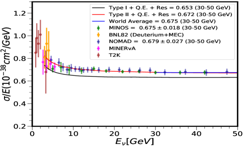
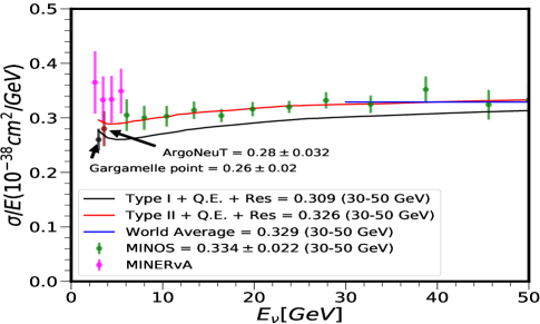
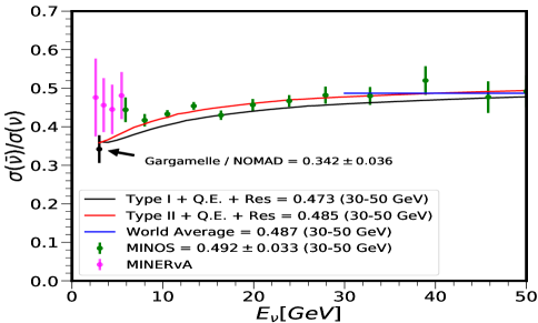
Figure 17: Model predictions (per nucleon) for an isoscalar iron target compared to measurements. The top part of the figure is for $\sigma_{\nu}$/E, the middle panel is for $\sigma_{\bar{\nu}}$/E, and the bottom panel is for the ratio $\sigma_{\bar{\nu}}$/$\sigma_{\nu}$ as a function of energy. The green points are MINOSMINOS2 data, and the blue points are NOMADNOMAD ; New_data_set $\sigma_{\nu}$/E measurments. The yellow crosses are BNL82BNL82 data as discussed in section 16. The MINERvAminerva1 and T2KT2K are shown in purple and brown, respectively. The GargamelleZeller ; GGM ; New_data_set and ArgoNeutargoneut of $\sigma_{\bar{\nu}}$/E per nucleon are identified. On the ratio plot we also show the Gargamelle antineutrino $\sigma_{\bar{\nu}}$/E at 3 GeV divided by the NOMAD neutrino $\sigma_{\nu}$/E at 4.6 GeV. The axial parameters of the Type II (A$>$V) model were tuned to agree with the total cross section data,

12.4 Comparisons to $\nu$ and $\overline{\nu}$ total cross section measurements for $E_{\nu}<$ 10 GeV

Because of quark hadron duality and the tuning of parameter described in section 12.2 the model also describes the $average$ cross section in the $1.4<W<1.8~{}GeV$ resonance region. As shown in Table 4, at an incident energy of 5 GeV, the contribution of the $1.4<W<1.8~{}GeV$ resonance region is significant. Therefore, comparison of our model predictions to low energy neutrino cross sections is a test of our modeling of the cross section in this resonance region.

Fig. 17 shows model predictions (per nucleon) for an isoscalar iron target that contains and equal number of protons and neutrons compared to measurements. The top panel is for $\sigma_{\nu}$/E, the middle panel is for $\sigma_{\bar{\nu}}$/E, and the bottom panel is for the ratio $\sigma_{\bar{\nu}}$/$\sigma_{\nu}$ as a function of energy.

The green points are MINOSMINOS2 data, and the blue points are NOMADNOMAD ; New_data_set $\sigma_{\nu}$/E measurements. The yellow crosses are BNL82BNL82 data as discussed in section 16. The MINERvAminerva1 and T2KT2K are shown in purple and brown, respectively. The GargamelleZeller ; GGM ; New_data_set and ArgoNeutargoneut of $\sigma_{\bar{\nu}}$/E per nucleon are identified. On the ratio plot we also show the Gargamelle antineutrino $\sigma_{\bar{\nu}}$/E at 3 GeV divided by the NOMAD neutrino $\sigma_{\nu}$/E at 4.6 GeV.

The Type II (A$>$V) red lines are the prediction of the Type II default model. The black lines are the prediction of the Type (A=V) model for which the axial structure functions are set equal to the vector structure functions. The blue lines above 30 GeV are the averages MINOS2 of all of the world’s data (on isoscalar iron) for energies between 30 and 50 GeV. The axial parameters of the Type II (A$>$V) default model were tuned to agree with the total cross section measurements.

For $\nu$ and $\overline{\nu}$ scattering, the Type II (A$>$V) default model describes the $1.4<W<1.8~{}GeV$ resonance region on $average$. However if a better resonance model is available, we suggest that it be used and smoothly matched to our model at $W>1.8$ GeV. Since our model also describes $average$ cross sections in the $1.4<W<1.8~{}GeV$ region, this matching should be continuous. In addition, comparisons of other resonance modesl predictions to our model in the $1.4<W<1.8~{}GeV$ region provides an estimate of the systematic errors associated with the modeling of the resonances.

13 Systematic errors in the application of the model

The model predicts neutrino cross sections at the Born level. Therefore, radiative corrections must be applied to the model if it is compared to non-radiatively corrected neutrino or charged-lepton scattering data. In general, all published charged-lepton scattering data are radiatively corrected. Similarly, published neutrino differential cross sections (e.g. CCFR, CDHSW, CHORUS, NuTeV) are radiatively corrected, and therefore can be directly compared to the model.

The model describes all inelastic charged-lepton scattering data and photoproduction on hydrogen and deuterium for $W>1.8~{}GeV$ at all values of $Q^{2}$ (and gives a reasonable $average$ cross section in the resonance region for $W>1.4~{}GeV$). Therefore, under the assumption of CVC, the model describes the vector part of the cross section in neutrino scattering well. The axial parameters of the Type II (A$>$V) default model were tuned to agree with the total cross section measurements.

Estimates of the systematic error in the total cross sections in Table 6 were obtained by varying the parameters in the model within our estimated uncertainties. in addition, a rough estimated of the uncertainties can be obtained by writing the differential cross sections in terms of quark and antiquark distributions. Within the naive quark parton model, the vector and axial structure functions are the same i.e. Type I (A=V) and the structure functions are related to the quark distribution by the following expressions:

$${\cal F}_{2}=2x[q(x,Q^{2})+\overline{q}(x,Q^{2})]$$

$$x{\cal F}_{3}=2[xq(x,Q^{2})-\overline{q}(x,Q^{2})]$$

We define $Q_{dist}(x,Q^{2})=2xq(x,Q^{2})$ and $\overline{Q}_{dist}(x,Q^{2})=2x\overline{q}(x,Q^{2})$. We define

$$Q_{T}=\int_{0}^{1}2xq(x,Q^{2})dx$$

$$\overline{Q}_{T}=\int_{0}^{1}2x\overline{q}(x,Q^{2})dx$$

.

The neutrino (antineutrino) differential cross section are then given by :

$$\frac{d^{2}\sigma^{\nu(\overline{\nu})}}{dxdy} = \frac{G_{F}^{2}ME}{\pi}$$ (53)

$$\times {\Big{(}}\Big{[}1-y(1+\frac{Mx}{2E})+\frac{y^{2}}{2}\frac{1+Q^{2}/\nu^{2}}{1+{\cal R}(x,Q^{2})}\Big{]}{\cal F}_{2}$$

$$\pm \Big{[}y-\frac{y^{2}}{2}\Big{]}x{\cal F}_{3}{\Big{)}}.$$

or

$$\frac{d^{2}\sigma^{\nu}}{dxdy} = \frac{G_{F}^{2}ME}{\pi}{\Big{(}}Q_{dist}(x,Q^{2})+(1-y)^{2}\overline{Q}_{dist}(x,Q^{2})$$

$$- \frac{y^{2}}{2}\frac{{\cal R}(x,Q^{2})}{1+{\cal R}(x,Q^{2})}(Q_{dist}+\overline{Q}_{dist})$$

$$+ \Big{[}-\frac{Mxy}{2E}+\frac{Mxy/E}{1+{\cal R}(x,Q^{2})}\Big{]}(Q_{dist}+\overline{Q}_{dist}){\Big{)}}.$$

and

$$\frac{d^{2}\sigma^{\overline{\nu}}}{dxdy} = \frac{G_{F}^{2}ME}{\pi}{\Big{(}}\overline{Q}_{dist}(x,Q^{2})+(1-y)^{2}Q_{dist}(x,Q^{2})$$

$$- \frac{y^{2}}{2}\frac{{\cal R}(x,Q^{2})}{1+{\cal R}(x,Q^{2})}(Q_{dist}+\overline{Q}_{dist})$$

$$+ \Big{[}-\frac{Mxy}{2E}+\frac{Mxy/E}{1+{\cal R}(x,Q^{2})}\Big{]}(Q_{dist}+\overline{Q}_{dist}){\Big{)}}.$$

Integrating over x and y, the cross sections for neutrino (anti-neutrino) (at high energy) can then be approximately expressed in terms of (on average) the fraction antiquarks $f_{\overline{Q}}=\overline{Q}_{T}/(Q_{T}+\overline{Q}_{T}$) in the nucleon, and (on average) the ratio of longitudinal to transverse cross sections ${\cal R}$ as follows:

$$\sigma(\nu N)\approx\frac{G_{F}^{2}ME}{\pi}(Q+\overline{Q})\Big{[}(1-f_{\overline{Q}})+\frac{1}{3}f_{\overline{Q}}-\frac{1}{6}\frac{{\cal R}}{(1+{\cal R)}}\Big{]},$$ (56)

and

$$\sigma(\overline{\nu}N\approx\frac{G_{F}^{2}ME}{\pi}(Q+\overline{Q})\Big{[}\frac{1}{3}(1-f_{\overline{Q}})+f_{\overline{Q}}-\frac{1}{6}\frac{{\cal R}}{(1+{\cal R)}}\Big{]}.$$ (57)

With $\langle{\cal R}\rangle=0.3$ at low $Q^{2}$ and $\langle f_{\overline{Q}}\rangle=0.175$, we obtain $\langle{\sigma_{\bar{\nu}}}/{\sigma_{\nu}}\rangle=0.487$, which is the world’s experimental average value in the 30-50 GeV energy range. The above expressions are only approximate. We use the exact expressions to estimate the systematic errors in the modeling the cross section originating from uncertainties in ${\cal R}$, uncertainties in $f_{\overline{q}}$, uncertainties in the axial K factors, and overall normalization. These are summarized in Table 6.

Table 6: Sources of systematic error in the predicted inelastic contribution to the total cross section on iron. The change (positive or negative) in the neutrino, antineutrino and the ${\sigma_{\bar{\nu}}}/{\sigma_{\nu}}$ ratio that originate from a plus one standard deviation change in the ratio of transverse to longitudinal structure functions (R), the fraction of antiquarks ($f_{\overline{q}}$), the difference between axial and vector K factors, and the overall normalization of the structure functions (N).

source	change	change	change	change
	(error)	in $\sigma_{\nu}$	in ${\sigma_{\bar{\nu}}}$	in ${\sigma_{\bar{\nu}}}/{\sigma_{\nu}}$
R	+0.1	-1.3%	-2.7%	-1.4%
$f_{\overline{Q}}$	+5%	-0.4%	+0.9%	+1.4%
$K^{axial}-K^{vector}$	-30%	-0.8%	-1.5%	-0.7%
Subtotal		$\pm 1.6\%$	$\pm 3.2\%$	$\pm 2.1\%$
N	+3%	+3%	+3%	0
Total		$\pm 3.4\%$	$\pm 4.4\%$	$\pm 2.1\%$
Experimental
uncertainties
in Total $\sigma$
measurements		$\pm 0.9\%$	$\pm 3.4\%$	$\pm 1.0\%$

We estimate the total systematic error in the modeling of the cross sections on iron for the $W>1.8~{}GeV$ region to be $\pm 3.4\%$ for neutrinos, $\pm 4.4\%$ for antineutrinos, and $\pm 2.1\%$ in the ${\sigma_{\bar{\nu}}}/{\sigma_{\nu}}$ ratio (for neutrino energies below 50 GeV). The errors are dominated by the PDF normalization errors of $\pm$3%. However, since the axial parameters were tuned to agree with the world’s total cross sections measurement, the smaller experimental uncertainties in the total cross section measurements shown in Table 6 may be taken as a lower limits of the systematic errors.

The following sources contribute to the systematic error.

1. Longitudinal structure function: In the analysis we use the ${\cal R}_{1998}$ parametrization. Preliminary results from the JUPITER Jefferson Lab collaboration indicates that ${\cal R}$ for heavy nucleus may be higher by about 0.1 than $R$ for deuterium. Therefore, we use an error of $\pm$0.1 in R to estimate the systematic error in the cross sections from this source.

2. The antiquark fraction in the nucleon ($f_{\overline{q}}$). We estimate an uncertainty of $\pm 5\%$ in the fraction of the sea quarks at low $Q^{2}$.

3. We assign a $\pm 3\%$ error in the overall normalization of the structure functions (N) on iron, partly from the error in normalization of the SLAC data on deuterium and partly from the level of consistency of the $Fe/D$ cross section ratio among the various measurement as seen in Fig.10.

4. Axial $K$ factors for sea and valence quarks: We use 30% of the difference between the cross section predictions of the Type I (A=V) and the Type II (A$>$V) models as an estimate of the uncertainty in the axial $K$ factors.

5. Charm sea: Since the GRV98 PDFs do not include a charm sea, the charm sea contribution must be added separately. This can be implemented either by using a boson-gluon fusion model, or by incorporating a charm sea from another set of PDFs. We modeled the contribution of the charm sea using a photon-gluon fusion model when we compared the predictions to photo-production data at HERA. If the charm sea contribution is neglected, the model underestimates the cross section at very high neutrino energies in the low $x$ and large $\nu$ region. For neutrino energies less than 50 GeV, the charm sea contribution is very small and can be neglected.

The following are additional sources of systematic errors which which are not included in Table 6.

• Nuclear corrections: The model is primarily a model for the structure functions of free nucleons. Only hydrogen and deuterium data are included in the fits.

• However, electron scattering data indicate that nuclear effects change the shape of the $x$ and $Q^{2}$ dependence of the structure functions of bound nucleons. Therefore in order to predict differential neutrino cross sections on heavy targets, we assume that the nuclear corrections are the same for the three structure functions. We also assume that the corrections are the same for the axial and vector contributions (and are equal to the nuclear corrections for ${\cal F}_{2}$ as measured in charged-lepton scattering), and that the nuclear corrections are only a function of $\xi_{TM}$ and are independent of $Q^{2}$. In general, nuclear corrections can be different for sea and valence quarks, and also for the longitudinal and transverse structure functions. Some of the systematic error in the modeling of the scattering from nuclear targets can be reduced when Jefferson Lab data on the nuclear dependence of ${\cal R}=\sigma_{L}/\sigma_{T}$ are published. Other systematic errors in the nuclear corrections can be reduced by assuming specific theoretical modelskulagin to account for the differences in the nuclear corrections between neutrino and charged-lepton scattering (as a function of $Q^{2}$ and $x$ for various nuclear targets).

$A$	$B$	$C_{v2d}$	$C_{v2u}$
$0.538$	$0.305$	$0.255$	$0.189$
$C_{sea}^{down}$	$C_{sea}^{up}$	$C_{v1d}$	$C_{v1u}$
$0.621$	$0.363$	$0.202$	$0.291$
$C_{sea}^{strange}$		${\cal F}_{valence}$	$N$
$0.621$		$[1-G_{D}^{2}(Q^{2})]$	$1.015$

Table 7: Parameters from NUINT04 version of the model which are currently implemented (with GRV98 PDFs) in the GENIE neutrino event generator. When applicable, all parameters are in units of GeV².

14 Updating the model in neutrino MC generators

The current (2016) version of the GENIEGENIE neutrino generator is using the NUINT04nuint04 version of the model. This early version of the model assumes that the axial structure functions are the same as the vector structure functions. As noted earlier, in this update, we refine the model and also account for the difference between the axial and vector structure functions at low values of $Q^{2}$. Table 7 shows the vector parameters of the NUINT04 version. Implementation of the 2021 Type II (A$>$V) default in neutrino MC generators can be done by updating the NUINT04 model as follows:

1. The vector parameters in Table 7 should be replaced by the vector parameters in table 2 (see equation 4).

2. The axial K factors as described in section 11 should be used for the axial structure functions.

3. Note that when the model implemented in neutrino Monte Carlo generators we must be careful not to double count the effect of Fermi motion. The above fits include the effect of Fermi motion at high $\xi_{TM}$. If Fermi motion is applied to the structure functions, than it is better to assume that the ratio of iron to deuterium without Fermi motion for $\xi_{TM}>0.65$ is equal to the ratio at $\xi_{TM}=0.65$.

4. The $K^{LW}_{vector}$ factor should be included for a better description in the resonance region. Here, $K^{LW}_{vector}=(\nu^{2}+C^{low-\nu}_{vector})/\nu^{2}$ (where $C^{low-\nu}_{vector}$=0.218) as shown in equation 4.

5. The $K^{LW-(\nu,\overline{\nu})}_{axial}$ factor should be included for a better description in the resonance region. Here,

   $$K^{LW-(\nu,\overline{\nu})}_{axial}=\frac{\nu^{2}+C_{axial}^{low-\nu(\nu,\overline{\nu})}}{\nu^{2}}$$

   For neutrinos:

   $$C^{low-\nu(\nu)}_{axial}=0.436.$$

   For antineutrinos

   $$C^{low-\nu(\overline{\nu})}_{axial}=0.654.$$

6. The structure function $x{\cal F}_{3}$ should be multiplied by the $H(,x,Q^{2})$ as described in equations 6 and 34.

7. The sea quark and antiquark contributions should be increased by 5% as shown in equation 2.

15 Tests of duality in the for QE and $\Delta$(1238) production

Table 8 shows a comparison of the sum of the measured $\sigma/E$ (in units of $10^{-39}~{}cm^{2}/GeV$) for QE and $\Delta(W<1.4)$ GeV, to the prediction of the Type II ($A>V$)(=BY II) model for $1.08<W<1.4$ GeV. The experimental errors for the QE and $\Delta$ cross sections are assumed to be 10%. The experimental cross sections are taken from Figures 18 and 19. The model predictions for the integrated cross section in the $1.08<W<1.4$ GeV region appears describe the $sum$ of the QE and the $\Delta(W<1.4)$ GeV measured cross sections.

$E_{\nu}$	$QE$	$W<1.4$	$1.08<W<1.4$
GeV		GeV	GeV	Ratio
		Δ(1238)	$\rm{}^{BY~{}II~{}model}$	${\rm{}^{BY~{}II/(QE+\Delta)}}$
3	1.83	1.57	3.72	1.09$\pm$0.15
5	1.10	0.92	2.25	1.1$\pm$0.16
10	0.53	0.45	1.13	1.16$\pm$0.16
40	0.13	0.11	0.30	1.21$\pm$0.17
$E_{\overline{\nu}}$	$QE$	$W<1.4$	$1.08<W<1.4$
GeV		GeV	GeV	Ratio
		Δ(1238)	$\rm{}^{BY~{}II~{}model}$	${\rm{}^{BY~{}II/(QE+\Delta)}}$
3	1.20	0.80	2.15	1.08$\pm$0.15
5	0.81	0.60	1.56	1.11 $\pm$0.16
10	0.46	10.35	0.90	1.11$\pm$0.16
40	0.13	0.10	0.27	1.20$\pm$0.17

Table 8: Test of duality: Comparison of the sum of the measured $\sigma/E$ (in units of $10^{-39}~{}cm^{2}/GeV$) for QE and $\Delta(W<1.4)$ GeV, to the prediction of the Type II ($A>V$)(=BY II) model for $1.08<W<1.4$ GeV. The experimental errors for the QE and $\Delta$ cross sections are assumed to be 10%. The model predictions for the integrated cross section in the $1.08<W<1.4$ GeV region appears describe the $sum$ of the QE and the $\Delta(W<1.4)$ GeV measured cross sections.

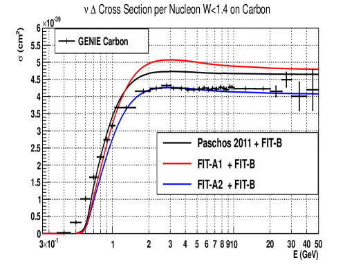
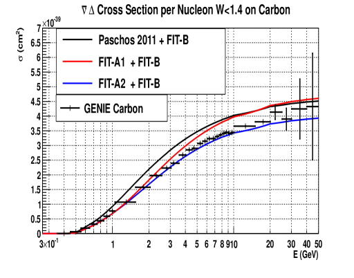
Figure 18: Figure from reference lownu . The total cross sections on carbon (per nucleon) predicted by GENIE for $W<1.4$ GeV (black points with MC statistical errors) for $\nu_{\mu}C\to(\mu^{-}\Delta^{++}$ or $\Delta^{+}$) are shown on the top panel, and for $\bar{\nu}_{\mu}C\to\mu^{+}(\Delta^{0}$ or $\Delta^{-}$) are shown on the bottom panel. The cross sections include the inelastic continuum for $W<1.4$ GeV. The red line and the green line span the range of experimental measurements of the cross sections for this region, as investigated in reference lownu . We take the midpoint between the red and green line as the best estimate of the cross sections for $W<1.4$ GeV (color online).

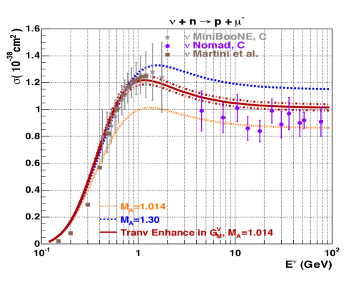
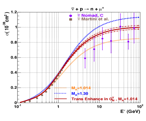
Figure 19: Figure from reference lownu . Comparison of predictions for the $\nu_{\mu}$, $\bar{\nu}_{\mu}$ total QE cross section sections from the nominal TE model lownu , the ”Independent Nucleon (MA=1.014)” model, the ”Larger $M_{A}$ ($M_{A}$=1.3) model”, and the ”QE+np-nh RPA” MEC model of Martini et al.MEC5 . We use the TE model to estimate the QE cross section. The data points are the measurements of MiniBooNEMiniBooNE (gray stars) and NOMADNOMAD (purple circles) (color online).

16 QE cross sections and cross section in the region of the $\Delta$ resonance ($W<1.4$ GeV)

16.1 cross section in the region of the $\Delta$ resonance ($W<1.4$ GeV)

Figure 18 is taken from reference lownu . The total cross sections on carbon (per nucleon) predicted by GENIE for $W<1.4$ GeV (black points with MC statistical errors) for $\nu_{\mu}C\to(\mu^{-}\Delta^{++}$ or $\Delta^{+}$) are shown on the top panel, and for $\bar{\nu}_{\mu}C\to\mu^{+}(\Delta^{0}$ or $\Delta^{-}$) are shown on the bottom panel. The cross sections include the inelastic continuum for $W<1.4$ GeV. The red line and the green line span the range of experimental measurements of the cross sections for this region, as investigated in reference lownu . We take the midpoint between the red and green line as the best estimate of the cross sections for $W<1.4$ GeV.

16.2 Neutrino and antineutrino quasielastic cross sections on nuclei

Figure 19 is taken from reference lownu . Shown are comparisons of predictions for the $\nu_{\mu}$, $\bar{\nu}_{\mu}$ total QE cross section sections from the nominal TE modellownu , the ”Independent Nucleon (MA=1.014)” model, the ”Larger $M_{A}$ ($M_{A}$=1.3) model”, and the ”QE+np-nh RPA” MEC model of Martini et al.MEC5 . The data points are the measurements of MiniBooNEMiniBooNE (gray stars) and NOMADNOMAD (purple circles). We use the TE model to estimate the QE cross section.

17 Appendix: The Adler sum rule

The Adler sum rules are derived from current algebra and are therefore valid at all values of $Q^{2}$. The equations below are for $strangeness~{}conserving(sc)$ processes. These are related to the PDFs by a factor of $cos^{2}\theta_{c}$.

The Adler sum rules for the vector part of the structure function ${\cal W}_{2}^{\nu-vector}$ is given by:

$$|F_{V}(Q^{2})|^{2}+\int_{\nu_{0}}^{\infty}{\cal W}_{2n-sc}^{\nu-vector}(\nu,Q^{2})d\nu$$ (58)

$$- \int_{\nu_{0}}^{\infty}{\cal W}_{2p-sc}^{\nu-vector}(\nu,Q^{2})d\nu=1,$$

where the limits of the integrals are from pion threshold $\nu_{0}$ where $W=M_{\pi}+M_{P}$ to $\nu=\infty$. At $Q^{2}=0$, the inelastic part of ${\cal W}_{2}^{\nu-vector}$ goes to zero, and the sum rule is saturated by the quasielastic contribution $|F_{V}(Q^{2})|^{2}$. Here $=Q^{2}/(4M^{2})$, and

$$|F_{V}(Q^{2})|^{2}-\frac{[G_{E}^{V}(Q^{2})]^{2}+\tau[G_{M}^{V}(Q^{2})]^{2}}{1+\tau}.$$

In the dipole approximation we have

$$G_{E}^{V}(Q^{2}) = G_{E}^{P}(Q^{2})-G_{E}^{N}(Q^{2})\approx G_{D}(Q^{2})$$ (59)

$$G_{M}^{V}(Q^{2}) = G_{M}^{P}(Q^{2})-G_{M}^{N}(Q^{2})\approx 4.706~{}G_{D}(Q^{2})$$ (60)

$$G_{D} = 1/(1+Q^{2}/M_{V}^{2})^{2},$$ (61)

where $M_{V}^{2}=0.71~{}GeV^{2}$. Note that in all of the calculations, we do not use the dipole approximation (we use BBBA2008  quasi vector and axial form factors).

The Adler sum rule for ${\cal W}_{2}^{\nu-axial}$ is given by:

$$|{\cal F}_{A}(Q^{2})|^{2}+\int_{\nu_{0}}^{\infty}{\cal W}_{2n-sc}^{\nu-axial}(\nu,Q^{2})d\nu$$

$$- \int_{\nu_{0}}^{\infty}{\cal W}_{2p-sc}^{\nu-axial}(\nu,Q^{2})d\nu=1,$$

where in the dipole approximation

$${\cal F}_{A}\approx-1.267/(1+Q^{2}/M_{A}^{2})^{2}$$

and $M_{A}=1.014~{}GeV$ from referencequasi .

The Adler sum rule for ${\cal W}_{1}^{\nu-vector}$ is given by:

$$\tau|G_{M}^{V}(Q^{2})|^{2}+\int_{\nu_{0}}^{\infty}{\cal W}_{1n}^{\nu-vector}(\nu,Q^{2})d\nu$$ (62)

$$- \int_{\nu_{0}}^{\infty}{\cal W}_{1p}^{\nu-vector}(\nu,Q^{2})d\nu=1.$$

The Adler sum rule for ${\cal W}_{1}^{\nu-axial}$ is given by:

$$(1+\tau)|{\cal F}_{A}(Q^{2})|^{2}+\int_{\nu_{0}}^{\infty}{\cal W}_{1n-sc}^{\nu-axial}(\nu,Q^{2})d\nu$$ (63)

$$- \int_{\nu_{0}}^{\infty}{\cal W}_{1p-sc}^{\nu-axial}(\nu,Q^{2})d\nu=1.$$

The Adler sum rule for ${\cal W}_{3}^{\nu}$ is given by:

$$2{\cal F}_{A}(Q^{2})G_{M}^{V}(Q^{2})+\int_{\nu_{0}}^{\infty}{\cal W}_{3n-sc}^{\nu}(\nu,Q^{2})d\nu$$ (64)

$$- \int_{\nu_{0}}^{\infty}{\cal W}_{3p-sc}^{\nu}(\nu,Q^{2})d\nu=0.$$

We use the Alder sum rule for ${\cal W}_{2}^{\nu-vector}$ to constrain the form of the $K_{valence}^{vector}(Q^{2})$ factor for ${\cal W}_{2}^{\nu-vector}$. At low $Q^{2}$ we approximate $|F_{V}(Q^{2})|^{2}$ by $G_{D}^{2}(Q^{2})$, and use the following $K$ factors for ${\cal W}_{2}^{\nu-vector}$.

$$K_{valence}^{vector}(Q^{2}) = [1-G_{D}^{2}(Q^{2})]\left(\frac{Q^{2}+C_{v2}}{Q^{2}+C_{v1}}\right),$$ (65)

where the values of the parameters $C_{v2d}$, $C_{v1d}$, $C_{v2u}$ and $C_{v1u}$ are obtained from a fit to the charged-lepton scattering and photoproduction data as discussed in section 3.

With this $K_{valence}^{vector}(Q^{2})$ factor, the Adler sum rule for ${\cal W}_{2}^{\nu-vector}$ is then approximately satisfied. At $Q^{2}=0$, the inelastic part of ${\cal W}_{2}^{\nu-vector}$ goes to zero, and the sum rule is saturated by the quasielastic contribution. Note that the contribution of the $\Delta(1232)$ resonance to the Adler sum rule is negative. Near $Q^{2}=0$ the $\Delta(1232)$ contribution is small in the vector case (since it must be zero at $Q^{2}=0$) and can be neglected. However, for the axial case the contribution of the $\Delta(1232)$at $Q^{2}=0$ is large and negative and cannot be neglected.

18 Appendix -Results with GRV94 PDFs

For completeness we describe the early NUINT01 analysis nuint01-2 in which we used another modified scaling variable  omegaw $x_{w}$ with GRV94 PDFs(instead of GRV98) and simplified $K$ factors. In that analysis we modified the leading order GRV94 PDFs as follows:

1. We increased the $d/u$ ratio at high $x$ as described in section 10 (and reference highx ).

2. Instead of the scaling variable $x$ we used the scaling variable $x_{w}=(Q^{2}+B)/(2M\nu+A)$ (or =$x(Q^{2}+B)/(Q^{2}+Ax)$). This modification was used in early fits to SLAC data bodek . The parameter A provides for an approximate way to include $both$ target mass and higher twist effects at high $x$, and the parameter B allows the fit to be used all the way down to the photoproduction limit ($Q^{2}$=0).

3. In addition as was done in earlier non-QCD based fits DL ; bonnie to low energy data, we multiplied all PDFs by a factor $K$=$Q^{2}$ / ($Q^{2}$ +C). This was done in order for the fits to describe low $Q^{2}$ data in the photoproduction limit, where ${\cal F}_{2}$ is related to the photoproduction cross section.

4. Finally, we froze the evolution of the GRV94 PDFs at a value of $Q^{2}=0.24$ (for $Q^{2}<0.24$), because GRV94 PDFs are only valid down to $Q^{2}=0.23~{}GeV^{2}$.

$A$	$B$	$C$	$\chi^{2}/ndf$
$1.735$	$0.624$	$0.188$	$1351/958$

Table 9: Parameters from NUINT01 version of the model (with GRV94 PDFs). When applicable, all parameters are in units of GeV².

In the GRV94 analysis, the measured structure functions were also corrected for the BCDMS magnetic field systematic error shiftbcdms and for the relative normalizations between SLAC, BCDMS and NMC data highx ; nnlo . The deuterium data were corrected for nuclear binding effects highx ; nnlo . A simultaneous fit to both proton and deuteron SLAC, NMC and BCDMS data (for $x>0.07$) yields the following values A=1.735, B=0.624 and C=0.188 GeV²) with GRV94 LO PDFs ($\chi^{2}=$ 1351/958 DOF). These parameters are summarized in Table 9. Note that for $x_{w}$ the parameter A accounts for $both$ target mass and higher twist effects.

In our studies with GRV94 PDFs we used the earlier ${\cal R}_{world}$ fit slac for ${\cal R}^{ncp}$ and ${\cal R}^{cp}$. ${\cal R}_{world}$ is parameterized by:

$${\cal R}_{world}(x,Q^{2}>0.35) = \frac{0.0635}{ln(Q^{2}/0.04)}\theta(x,Q^{2})$$ (66)

$$+ \frac{0.5747}{Q^{2}}-\frac{0.3534}{Q^{4}+0.09},$$

where $\theta=1.+\frac{12Q^{2}}{Q^{2}+1.0}\times\frac{0.125^{2}}{0.125^{2}+x^{2}}$. The ${\cal R}_{world}$ function provided a good description of the world’s data for ${\cal R}$ at that time in the $Q^{2}>0.35$ $GeV^{2}$ and $x>0.05$ region (where most of the ${\cal R}$ data are available). However, for electron and muon scattering and for the vector part of neutrino scattering the ${\cal R}_{world}$ function breaks down below $Q^{2}=0.35$ $GeV^{2}$.

Here, we freeze the function at $Q^{2}=0.35$ GeV². For electron and muon scattering and for the vector part of ${\cal F}_{1}$ we introduce a $K$ factor for ${\cal R}$ in the $Q^{2}<0.35$ GeV² region. The $K$ factor provides a smooth transition for the vector ${\cal R}$ (we use ${\cal R}_{vector}$=${\cal R}_{e/\mu}$) from $Q^{2}=0.35$ GeV² down to $Q^{2}=0$ by forcing ${\cal R}_{vector}$ to approach zero at $Q^{2}=0$ as expected in the photoproduction limit (while keeping a $1/Q^{2}$ behavior at large $Q^{2}$ and matching to ${\cal R}_{world}$ at $Q^{2}=0.35$ GeV²).

$${\cal R}_{vector}(x,Q^{2}<0.35) = 3.207\times\frac{Q^{2}}{Q^{4}+1}$$

$$\times {\cal R}_{world}(x,Q^{2}=0.35).$$

19 Acknowlegements

Research supported by the U.S. Department of Energy under grant number DE-SC0008475 and Promising-Pioneering Researcher Program through Seoul National University.f

References

- (1) S. Fukuda et al., Phys. Rev. Lett. 85, 3999 (2000); T. Toshito, hep-ex/0105023.
- (2) D.G. Michael et al.(MINOS), Phys. Rev. Lett. 97, 191801 (2006); http://www-numi.fnal.gov/Minos/
- (3) P. Adamson et al.(MINOS), Phys. Rev. D 81, 072002 (2010).
- (4) P. Adamson et al.(NOVA, Phys. Rev. D 93 051104 (2016 )( http://www-nova.fnal.gov/)
- (5) M. H. Ahn et al.(K2K), Phys. Rev. D 74, 072003 (2006); http://neutrino.kek.jp/
- (6) Y. Ashie et al.(SuperK), Phys. Rev. D 71, 112005 (2005);
- (7) K. Abe et al. (T2K), Phys. Rev. D 87, 092003 (2013); K. Abe et al. (T2K), Phys. Rev. D 90, 052010 (2014); K. Abe et al. (T2K), Phys. Rev. D 93, 072002 (2016). We applied Isoscalar correction from ref. minerva1 to T2K total cross sections.
- (8) A. A. Aguilar-Arevalo et al.(MiniBooNE), Phys. Rev. Lett 98, 231801(2007)
- (9) The DUNE Collaboration, B. Abi et al. ”The DUNE Far Detector Interim Design Report Volume 1: Physics, Technology and Strategies” arXiv:1807.10334 [physics.ins-det]
- (10) Y. Nakjima et al., (SciBoonE) arXiv:hep-ex/1011.213
- (11) MicroBooNE collaboration, ?Design and Construction of the MicroBooNE Detector?, arXiv:1612.05824, JINST 12, P02017 (2017)
- (12) R. Acciarri et al. (ArgoNeuT), Phys. Rev. D 89, 112003 (2014).
- (13) J. DeVan et. al. (MINERvA) Phys. Rev. D 94, 112007 (2016) arXiv:1610.04746
- (14) ICARUS at Fermilab, https://icarus.fnal.gov/
- (15) A. Bodek and U.K. Yang (NUINT01),Nucl. Phys. B Proc. Suppl.112, 70 (2002), arXiv:hep-ex/0203009; A. Bodek and U. K. Yang (NUINT02), arXiv:hep-ex/0308007.
- (16) A. Bodek , Ikyu Park and U. K. Yang, (NUINT04) Nucl. Phys. B Proc. Suppl.139, 113 (2005), arXiv:hep-ph/0411202.
- (17) Y. Hayato, Nucl Phys. Proc. Suppl.. 112, 171 (2002)
- (18) C.Andreopoulos (GENIE), Nucl. Instrum. Meth. A614, 87 (2010)
- (19) H. Gallagher (NEUGEN), Nucl. Phys. Proc. Suppl. 112 (2002)
- (20) D. Casper (NUANCE) , Nucl. Phys. Proc. Suppl. 112, 161 (2002); http://nuint.ps.uci.edu/nuance/
- (21) U. K. Yang and A. Bodek, Phys. Rev. Lett. 82, 2467 (1999)
- (22) U. K. Yang and A. Bodek, Eur. Phys. J. C13, 241 (2000)
- (23) U. K. Yang, Ph.D. thesis, Univ. of Rochester (2001), FERMILAB-THESIS-2001-09, available at .
- (24) L.W. Whitlow, E.M. Riordan, S. Dasu, S. Rock, A. Bodek (SLAC-MIT), Phys. Lett. B282, 433 (1995); L.W. Whitlow, PhD thesis, Stanford University, SLAC Report 357 (1990)
- (25) A. C. Benvenuti et al. (BCDMS), Phys. Lett. B237, 592 (1990); M. Virchaux and A. Milsztajn, Phys. Lett. B 274, 221 (1992)
- (26) M. Arneodo et al. (NMC), Nucl. Phys. B483, 3 (1997)
- (27) R. Barbieri et al., Phys. Lett. B64, 171 (1976), and Nucl. Phys. B117, 50 (1976)
- (28) O. Nachtmann, Nucl. Phys. B63 (1973) 237; O. Nachtmann, Nucl. Phys. B78 (1974) 455; O. W. Greenberg and D. Bhaumik, Phys. Rev. D4 (1971) 2048; H. Georgi and H. D. Politzer, Phys. Rev. D14, 1829 (1976); J. Pestieau and J. Urias, Phys.Rev.D8, 1552 (1973)
- (29) M. Gluck, E. Reya, A. Vogt, Eur. Phys. J C5, 461 (1998).
- (30) A. Donnachie and P. V. Landshoff, Z. Phys. C 61, 139 (1994).
- (31) B. T. Fleming et al.(CCFR), Phys. Rev. Lett. 86, 5430 (2001).
- (32) F. W. Brasse et al., Nucl. Phys. B 839, 421 (1972).
- (33) A. Bodek et al., Phys. Rev. D20, 1471 (1979).
- (34) S. Stein et al., Phys. Rev. D12, 1884 (1975); K. Gottfried, Phys. Rev. Lett. 18, 1174 (1967).
- (35) S. Adler, Phys. Rev. 143, 1144 (1966); F. Gillman, Phys. Rev. 167, 1365 (1968).
- (36) O. Lalakulich, W. Melnitchouk, and E. A. Paschos, Phys. Rev. C 75,015202 (2007).
- (37) C. Adloff et al. (H1) , Eur Phys J C30, 32 (2003); http://www-h1.desy.de/
- (38) Photoproduction: David O. Caldwell, et al. Phys. Rev. Lett. 25, 609 (1970); T.A. Armstrong et al. Nucl. Phys. B41, 445 (1972); T.A. Armstrong et al. Phys. Rev. D5, 1640 (1972); David O. Caldwell, et al. Phys. Rev. D7, 1362 (1973) (nuclear targets); David O. Caldwell et al. Phys. Rev. Lett. 40, 1222, (1978); S. Chekanov et al. (ZEUS) Nucl. Phys. B627, 3 (2002); T. Ahmed et al. (H1) Phys. Lett. B299 374 (1993).
- (39) C. Keppel, Proc. of the Workshop on Exclusive Processes at High , Newport News, VA, May (2002).
- (40) E. D. Bloom and F. J. Gilman, Phys. Rev. Lett. 25, 1140 (1970).
- (41) Y. Liang et al.(E94-110), arXiv:nucl-ex/0410027.
- (42) K. Abe et al., Phys. Lett. B452, 194 (1999)
- (43) R.S. Thorne and R.G. Roberts, Phys. Lett. B 421, 303 (1998); Eur. Phys. J. C 19, 339 (2001).
- (44) S. A. Kulagin and R. Pett, Phys. Rev. D76, 094023 (2007), ibid Nucl. Phys. A765, 26 (2006).
- (45) P.E. Bosted and M.E. Christy, Phys. Rev. C77, 065206 (2008); M.E. Christy and P.E. Bosted, Phys. Rev. C81, 055213 (2010), arXiv:0712.3731. Fortran program for ia available at .
- (46) W. G. Seligman, Ph.D. thesis, (CCFR) Columbia Univ., Nevis reports 292 (1997).
- (47) J. Arrington et al (Jefferson Lab), Phys.Rev. C73, 035205 (2006).
- (48) A. Bodek et al. (E87), Phys. Rev. Lett. 50, 1431 (1983).
- (49) J. Gomez et al. (E139, Phys. Rev. D49, 4348 (1994).
- (50) S. Dasu et al. (E140) , Phys. Rev. Lett. 60, 2591 (1988); S. Dasu et al. (E140) Phys. Rev. D 49, 5641 (1994).
- (51) M. Arneodo (NMC)et al., Nucl. Phys. B 481, 3 (1966).
- (52) R. Seely et al. (Jefferson Lab data on Carbon), Phys. Rev. Lett. 103, 202301 (2009).
- (53) R. Oldeman, Proc. of 30th International Conference on High-Energy Physics (ICHEP 2000), Osaka, Japan, 2000; R. G. C. Oldeman, Ph.D. thesis, University of Amsterdam, 2000; G. Onengut et al. (CHORUS ) Phys.Lett. B632, 65 (2006). http://choruswww.cern.ch/Publications/DIS-data
- (54) U. K. Yang et al.(CCFR), Phys. Rev. Lett. 87, 251802 (2001).
- (55) P. Berge et al. (CDHSW), Zeit. Phys. C49, 607 (1991).
- (56) A. Bodek, S. Avvakumov, R. Bradford, and H. Budd, Eur. Phys. J. C53, 349 (2008).
- (57) A. Bodek , U. Sarica, D. Naples and L. Ren, Eur.Phys.J.C 72 (2012) 1973
- (58) V. Lyubushkin et al. (NOMAD Collaboration), Eur. Phys. J. C 63, 355 (2009); Q. Wu et al.(NOMAD Collaboration), Phys. Lett. B60, 19 (2008).
- (59) V.B. Anikeev, et al. (Serpukhov) Z. Phys. C 70, 39 (1996)
- (60) N. J. Baker et al. (BNL) Phys. Rev. D 25, 617 (1982).
- (61) M. Martini, M. Ericson, G. Chanfray, and J. Marteau, Phys. Rev. C 80: 065501, 2009; ibid Phys. Rev. C 81: 045502, 2010.
- (62) J.A. Formaggio, G.P. Zeller, Rev. Mod. Phys. 84, 1307 (2012) (arXiv:1305.7513 [hep-ex])
- (63) Ciampolillo, S., et al. (Gargamelle Neutrino Propane Collaboration, Aachen-Brussels-CERN-Ecole Poly-Orsay-Padua Collaboration), 1979, Phys.Lett. B84, 281.
- (64) M.R. Whalley, Nucl.Phys.B Proc.Suppl. 139 (2005) 241 (hep-ph/0410399)