On non-factorisable contributions to $t$-channel single-top production

Abstract

We compute the non-factorisable contribution to the two-loop helicity amplitude for $t$-channel single-top production, the last missing piece of the two-loop virtual corrections to this process. Our calculation employs analytic reduction to master integrals and the auxiliary mass flow method for their fast numerical evaluation. We study the impact of these corrections on basic observables that are measured experimentally in the single-top production process.

1 Introduction

Hadronic production of top quarks at the LHC provides an opportunity to study the heaviest particle of the Standard Model in great detail. Since, according to the Standard Model, top quarks receive their masses exclusively through interactions with the Higgs background field, a better understanding of top quark properties may lead to a better understanding of electroweak symmetry breaking in and, hopefully, beyond, the Standard Model.

At a hadron collider top quarks and anti-quarks are primarily produced in pairs by means of strong interactions. However, single-top production, which necessarily involves the weak $tWb$ interaction vertex, also occurs quite frequently at the LHC. In fact, the single-top production cross section at the LHC is about a quarter of the cross section to produce a $t\bar{t}$ pair. Such a large cross section and an impressive luminosity collected at the LHC implies that by now ${\cal O}(10)$ millions top quarks have been produced there thanks to this mechanism.

The interest in single-top production is related to the fact that weak interactions are responsible for this process. This opens up a number of interesting opportunities Giammanco:2017xyn that involve studies of the structure of the $tbW$ vertex ATLAS:2017ygi ; ATLAS:2019hhu , improving constrains on the CKM matrix elements CMS:2020vac ; ATLAS:2019hhu and indirect determination of the top quark width $\Gamma_{t}$ CMS:2014mxl . More recently, measurements of the top quark mass in single-top events started to play a more visible role in the top quark mass measurements at the LHC CMS:2017mpr . Finally, detailed studies of QCD dynamics in single-top production processes including interesting constraints on parton distribution functions and precise measurements of kinematic distributions are benefitting from the high integrated luminosity of the LHC CMS:2019jjp ; ATLAS:2017rso .

At a hadron collider, single top quarks can be produced in three different ways (for a review, see Ref. Giammanco:2017xyn ). One distinguishes i) the $t$-channel process that refers to $q\,b\to q^{\prime}\,t$ scattering mediated by an exchange of a $W$ boson, ii) the $s$-channel process that at the partonic level corresponds to $q\,\overline{q^{\prime}}\to W^{*}\to t\,\overline{b}$ and, finally, iii) the associated production that involves the $g\,b\to W\,t$ process. About $70\%$ of single top quarks at the LHC are produced in the $t$-channel process; ${\cal O}(25\%)$ are due to the associated $tW$ production and only ${\cal O}(5\%)$ are due to the $s$-channel process.

Studies of single-top production rely on a precise theoretical description of this process that can be obtained in the context of perturbative QCD and collinear factorisation. This has been done at next-to-leading order (NLO) in perturbative QCD in Refs. Harris:2002md ; Campbell:2004ch ; Sullivan:2004ie ; Cao:2004ky ; Schwienhorst:2010je ; Gao:2021plf . Furthermore, for the $t$-channel production next-to-next-to-leading order (NNLO) QCD corrections have been calculated in Refs. Brucherseifer:2014ama ; Berger:2016oht ; Campbell:2020fhf . Although the more recent computations of such corrections presented in Refs. Berger:2016oht ; Campbell:2020fhf are quite sophisticated and incorporate top quark decays and QCD corrections to them in the narrow width approximation, all existing calculations of NNLO QCD corrections to $t$-channel single-top production do not account for the so-called non-factorisable contributions.

In the context of $t$-channel single-top production, non-factorisable corrections refer to contributions that connect a light-quark line and a heavy $b\to t$ line by gluon exchanges, see Figure 1. Thanks to colour conservation, such contributions vanish when NLO QCD predictions for cross sections are computed. However, since at next-to-next-to-leading order two gluons in a colour-singlet state can be exchanged between different fermion lines, non-factorisable diagrams start contributing at that order and, in principle, have to be accounted for.

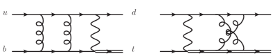
Figure 1: Examples of non-factorisable two-loop diagrams. Wavy lines represent $W$ bosons, curly lines are gluons, solid lines are quarks. The double line represents the top quark.

However, it is far from obvious that these non-factorisable corrections are important for a precise description of single-top production. The reason for neglecting them in earlier computations was that they are colour-suppressed compared to factorisable contributions shown in Figure 2. On the other hand, as became clear recently, these non-factorisable corrections may be enhanced by a factor $\pi^{2}$ related to remnants of the so-called Coulomb or Glauber phase glauber . Indeed, the existence of such an enhancement was recently demonstrated Liu:2019tuy in the context of Higgs boson production in weak boson fusion. In fact it was shown in that reference that the $\pi^{2}$-enhancement of non-factorisable corrections largely compensates their ${\cal O}(1/N_{c}^{2})$ suppression, so that the non-factorisable corrections to Higgs production in weak boson fusion are larger than the colour-suppression argument suggests. Moreover, it is known that factorisable NNLO QCD corrections to single-top production cross section and basic kinematic distributions are rather small Brucherseifer:2014ama ; Berger:2016oht ; Campbell:2020fhf . This smallness of factorisable QCD corrections makes non-factorisable corrections more relevant provided, of course, that high-precision theoretical description of single-top production is of interest.

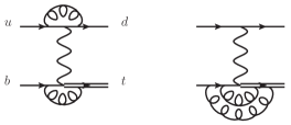
Figure 2: Examples of factorisable two-loop diagrams not considered in the present calculation. Wavy lines represent $W$ bosons, curly lines are gluons, solid lines are quarks. The double line represents the top quark.

The goal of this paper is to make the first step towards a better understanding of non-factorisable corrections to single-top production at the LHC and to calculate their contributions to the two-loop virtual amplitude. We do this by expressing all two-loop integrals that appear in non-factorisable diagrams through master integrals keeping exact dependence on the top quark mass and the $W$ mass and by computing these integrals using the auxiliary mass flow method Liu:2017jxz ; Liu:2020kpc ; Liu:2021wks . As we explain in detail below, this computational set up is similar to the one used previously by two of the present authors Bronnum-Hansen:2020mzk ; Bronnum-Hansen:2021olh .

This paper is organised as follows. In Section 2 we discuss technical details pertinent to the calculation of non-factorisable contributions to the single-top production amplitude. In Section 3 we describe the numerical evaluation of the master integrals. The (infrared) pole structure of the non-factorisable contribution to the amplitude is discussed in Section 4. The impact of non-factorisable corrections on the cross section and some kinematic distributions are studied in Section 5. We conclude in Section 6. Numerical values for non-factorisable contributions to the two-loop amplitude at a few kinematic points are presented in Appendix A. Boundary conditions for master integrals that we used in this calculation can be found in an ancillary file.

2 Non-factorisable contributions to helicity amplitudes

We consider single-top production in the $t$-channel and, for definiteness, focus on a particular flavour of light quarks

$$u(p_{1})+b(p_{2}) \to d(p_{3})+t(p_{4}).$$ (1)

Except for the top quark, all other quarks in Eq. (1) are massless, so that $p_{i}^{2}=0,\ i=1,2,3$. The top quark is on the mass-shell $p_{4}^{2}=m_{t}^{2}$. We follow standard conventions and define Mandelstam variables as

$$s=(p_{1}+p_{2})^{2},\qquad t=(p_{1}-p_{3})^{2},\qquad u=(p_{2}-p_{3})^{2},$$ (2)

with $s+t+u=m_{t}^{2}$.

We write the amplitude of the process in Eq. (1) expanded in the renormalised strong coupling constant $\alpha_{s}=\alpha_{s}(\mu)$ as follows

$$\mathcal{A}(\{p_{i}\})=g_{w}^{2}V_{ud}V_{tb}\left(\mathcal{A}^{(0)}+\frac{\alpha_{s}}{4\pi}\mathcal{A}_{\rm nf}^{(1)}+\left(\frac{\alpha_{s}}{4\pi}\right)^{2}\mathcal{A}_{\rm nf}^{(2)}+...+\mathcal{O}\left(\alpha_{s}^{3}\right)\right)\,.$$ (3)

When writing Eq. (3), we have extracted the weak coupling constant $g_{w}$ and the CKM matrix elements $V_{tb}$ and $V_{ud}$. Also, $\mathcal{A}^{(0)}=\mathcal{A}^{(0)}(\{p_{i}\})$ is the (properly normalised) Born amplitude of the process Eq. (1), $\mathcal{A}_{\rm nf}^{(1,2)}=\mathcal{A}_{\rm nf}^{(1,2)}(\{p_{i}\})$ are one- and two-loop non-factorisable amplitudes respectively, and ellipses stand for factorisable contributions that we do not discuss in this paper.

To proceed further, we perform the colour decomposition of relevant amplitudes. Figure 3 shows the only diagram that contributes to $t$-channel single-top production at tree level. Since $W$ bosons carry no colour charge, we find

$$\mathcal{A}^{(0)}=\hat{1}_{c_{3}c_{1}}\hat{1}_{c_{4}c_{2}}A^{(0)}=\delta_{c_{1}c_{3}}\delta_{c_{2}c_{4}}\,A^{(0)},$$ (4)

where $\hat{1}$ is the identity matrix, $c_{1,..,4}$ are the colour indices of particles with momenta $p_{1,..,4}$, respectively, and $A^{(0)}$ is the colour-stripped amplitude.

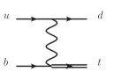
Figure 3: Tree-level diagram. Wavy lines represent $W$ bosons, solid lines are quarks. The double line represents the top quark.

Four box diagrams with identical colour factors contribute to the one-loop non-factorisable amplitude. We write

$$\mathcal{A}_{\rm nf}^{(1)}=T^{a}_{c_{3}c_{1}}T^{a}_{c_{4}c_{2}}A_{\rm nf}^{(1)}=\frac{1}{2}\left(\delta_{c_{1}c_{4}}\delta_{c_{2}c_{3}}-\frac{1}{N_{c}}\delta_{c_{1}c_{3}}\delta_{c_{2}c_{4}}\right)A_{\rm nf}^{(1)}.$$ (5)

We note that the interference of the one-loop amplitude and the Born amplitude vanishes thanks to colour conservation

$$\sum_{\text{colour}}\mathcal{A}^{(0)\star}\mathcal{A}_{\rm nf}^{(1)}=0.$$ (6)

At two loops eighteen non-factorisable box diagrams need to be considered; we generate them using QGRAF Nogueira:1991ex . Since $W$ bosons are colourless, these diagrams are of both planar and non-planar types as far as QCD interactions are concerned. For this reason, there are just two distinct colour factors

$$c_{2,\rm pl}=(T^{a}T^{b})_{c_{3}c_{1}}(T^{a}T^{b})_{c_{4}c_{2}},\;\;\;\;c_{2,\rm npl}=(T^{a}T^{b})_{c_{3}c_{1}}(T^{b}T^{a})_{c_{4}c_{2}},\;\;\;\;$$ (7)

so that

$$\mathcal{A}_{\rm nf}^{(2)}=c_{2,\rm pl}A_{\rm nf}^{(2),\rm pl}+c_{2,\rm npl}A_{\rm nf}^{(2),\rm npl}.$$ (8)

The two amplitudes $A_{\rm nf}^{(2),\rm pl}$ and $A_{\rm nf}^{(2),\rm npl}$ are obtained by computing (QCD) planar and non-planar diagrams, respectively.

However, it is easy to realise that only a particular combination of these amplitudes contributes to NNLO QCD cross section through interference with the leading-order amplitude. Indeed, since the leading-order colour factor involves $\delta_{c_{3}c_{1}}\delta_{c_{4}c_{2}}$, when the interference of non-factorisable two-loop diagrams and the tree amplitude is computed, we obtain ${\rm Tr}(T^{a_{1}}T^{a_{2}})$ for each of the fermion lines. However, since ${\rm Tr}(T^{a}T^{b})={\rm Tr}(T^{b}T^{a})$, the distinction between colour factors for planar and non-planar diagrams disappears. To project on the relevant structure, we write

$$2T^{a}T^{b}=\{T^{a},T^{b}\}+[T^{a},T^{b}],\;\;\;2T^{b}T^{a}=\{T^{a},T^{b}\}-[T^{a},T^{b}].\;\;\;$$ (9)

Since ${\rm Tr}\left([T^{a},T^{b}]\right)=0$, commutators of colour generators do not contribute to the interference. As the result, we can write

$$\begin{split}\mathcal{A}_{\rm nf}^{(2)}&=\frac{1}{4}\{T^{a},T^{b}\}_{c_{3}c_{1}}\{T^{a},T^{b}\}_{c_{4}c_{2}}\;(A_{\rm nf}^{(2),\rm pl}+A_{\rm nf}^{2,\rm npl})+\dots\\ &=\frac{1}{4}\{T^{a},T^{b}\}_{c_{3}c_{1}}\{T^{a},T^{b}\}_{c_{4}c_{2}}\;A_{\rm nf}^{(2)}+\dots,\end{split}$$ (10)

where ellipses stand for terms that vanish when the interference of $\mathcal{A}_{\rm nf}^{(2)}$ with tree amplitude is computed. We note that we introduced $A_{\rm nf}^{(2)}=A_{\rm nf}^{(2),\rm pl}+A_{\rm nf}^{2,\rm npl}$ in Eq. (10). We find

$$\sum_{\text{colour}}\mathcal{A}^{(0)*}\mathcal{A}_{\rm nf}^{(2)}=\frac{1}{4}(N_{c}^{2}-1)\;A^{(0)*}A_{\rm nf}^{(2)}.$$ (11)

To compute relevant one- and two-loop amplitudes, we need to write them in terms of invariant form factors and independent Lorentz structures. Since charged weak currents involve left-handed projectors and, therefore, the Dirac matrix $\gamma_{5}$, care is needed when performing computations in dimensional regularisation. However, since no closed fermion loops contribute to non-factorisable corrections, we can make use of an anti-commuting prescription for the $\gamma_{5}$ and move left-handed projectors to act on the external massless fermion states. It then becomes clear that we can consider amplitudes mediated by the vector current but only account for left-handed massless quarks when constructing physical amplitudes for the charged current.

There are eleven structures that may contribute to the non-factorisable part of the amplitude through NNLO QCD. They are

$$\begin{split}&{\cal S}_{1}=\overline{u}_{t}({p_{4}})\,\,u({p_{2}})\times\overline{u}({p_{3}})\,\not{p}_{4}\,u({p_{1}})\,,\\ &{\cal S}_{2}=\overline{u}_{t}({p_{4}})\,\not{p}_{1}\,u({p_{2}})\times\overline{u}({p_{3}})\,\not{p}_{4}\,u({p_{1}})\,,\\ &{\cal S}_{3}=\overline{u}_{t}({p_{4}})\,\gamma^{\mu_{1}}\,u({p_{2}})\times\overline{u}({p_{3}})\,\gamma_{\mu_{1}}\,u({p_{1}})\,,\\ &{\cal S}_{4}=\overline{u}_{t}({p_{4}})\,\gamma^{\mu_{1}}\not{p}_{1}\,u({p_{2}})\times\overline{u}({p_{3}})\,\gamma_{\mu_{1}}\,u({p_{1}})\,,\\ &{\cal S}_{5}=\overline{u}_{t}({p_{4}})\,\gamma^{\mu_{1}}\gamma^{\mu_{2}}\,u({p_{2}})\times\overline{u}({p_{3}})\,\gamma_{\mu_{1}}\gamma_{\mu_{2}}\not{p}_{4}\,u({p_{1}})\,,\\ &{\cal S}_{6}=\overline{u}_{t}({p_{4}})\,\gamma^{\mu_{1}}\gamma^{\mu_{2}}\not{p}_{1}\,u({p_{2}})\times\overline{u}({p_{3}})\,\gamma_{\mu_{1}}\gamma_{\mu_{2}}\not{p}_{4}\,u({p_{1}})\,,\\ &{\cal S}_{7}=\overline{u}_{t}({p_{4}})\,\gamma^{\mu_{1}}\gamma^{\mu_{2}}\gamma^{\mu_{3}}\,u({p_{2}})\times\overline{u}({p_{3}})\,\gamma_{\mu_{1}}\gamma_{\mu_{2}}\gamma_{\mu_{3}}\,u({p_{1}})\,,\\ &{\cal S}_{8}=\overline{u}_{t}({p_{4}})\,\gamma^{\mu_{1}}\gamma^{\mu_{2}}\gamma^{\mu_{3}}\not{p}_{1}\,u({p_{2}})\times\overline{u}({p_{3}})\,\gamma_{\mu_{1}}\gamma_{\mu_{2}}\gamma_{\mu_{3}}\,u({p_{1}})\,,\\ &{\cal S}_{9}=\overline{u}_{t}({p_{4}})\,\gamma^{\mu_{1}}\gamma^{\mu_{2}}\gamma^{\mu_{3}}\gamma^{\mu_{4}}\,u({p_{2}})\times\overline{u}({p_{3}})\,\gamma_{\mu_{1}}\gamma_{\mu_{2}}\gamma_{\mu_{3}}\gamma_{\mu_{4}}\not{p}_{4}\,u({p_{1}})\,,\\ &{\cal S}_{10}=\overline{u}_{t}({p_{4}})\,\gamma^{\mu_{1}}\gamma^{\mu_{2}}\gamma^{\mu_{3}}\gamma^{\mu_{4}}\not{p}_{1}\,u({p_{2}})\times\overline{u}({p_{3}})\,\gamma_{\mu_{1}}\gamma_{\mu_{2}}\gamma_{\mu_{3}}\gamma_{\mu_{4}}\not{p}_{4}\,u({p_{1}})\,,\\ &{\cal S}_{11}=\overline{u}_{t}({p_{4}})\,\gamma^{\mu_{1}}\gamma^{\mu_{2}}\gamma^{\mu_{3}}\gamma^{\mu_{4}}\gamma^{\mu_{5}}\,u({p_{2}})\times\overline{u}({p_{3}})\,\gamma_{\mu_{1}}\gamma_{\mu_{2}}\gamma_{\mu_{3}}\gamma_{\mu_{4}}\gamma_{\mu_{5}}\,u({p_{1}})\,,\end{split}$$ (12)

where $u_{t}({p_{4}})$ denotes the only massive spinor. We note that the above quantities depend on the polarisation states of external fermions that, in what follows, we will denote by $\vec{\lambda}$. Therefore, we will write ${\cal S}_{i}={\cal S}_{i}(\vec{\lambda})$, $i=1,\dots,11$.

It is clear that not all eleven structures contribute at leading and next-to-leading order in the perturbative expansion of the amplitude ${\cal A}$. Indeed, at tree level each fermion line has exactly one Dirac matrix. As the result, the colour-stripped tree-level amplitude for the $u+b\to d+t$ process can be written as

$$A^{(0)}(\vec{\lambda})=\frac{{\cal S}_{3}(\vec{\lambda})}{4(t-m_{W}^{2})}\,.$$ (13)

Upon squaring $\mathcal{A}^{(0)}(\vec{\lambda})$ and summing over colours and appropriate polarisation states of external fermions, we find

$$\sum_{\vec{\lambda},\rm colours}|\mathcal{A}^{(0)}(\vec{\lambda})|^{2}=N_{c}^{2}\frac{4s(s-m_{t}^{2})}{(t-m_{W}^{2})^{2}}\,.$$ (14)

The one-loop diagrams have at most three $\gamma$-matrices on each fermion line and can therefore be decomposed in terms of the first seven tensor structures. At two loops we need all eleven structures to express the amplitude in terms of invariant form factors. We write

$$A_{\rm nf}^{(2)}=\vec{f}\cdot\vec{\mathcal{S}},$$ (15)

where we introduced vectors $\vec{\cal{S}}$ and $\vec{f}$ to accommodate eleven tensor structures $\vec{\cal{S}}^{T}=({\cal S}_{1},{\cal S}_{2},\dots,{\cal S}_{11})$ and eleven form factors, respectively.

To compute the form factors, we calculate eleven quantities

$$Q_{i}=\sum_{\vec{\lambda}}{\cal S}_{i}^{\dagger}(\vec{\lambda})\,A^{(2)}_{\rm nf}(\vec{\lambda}),\;\;\;i=1,\dots,11,$$ (16)

where the sum runs over all polarisation states of external fermions. We stress that since form factors do not depend on helicities of external quarks, we do not need to restrict polarisation states to left-handed ones when computing the sum in Eq. (16). Hence, we can use simple formulas to describe density matrices of external quarks

$$\sum_{\lambda}u(p_{i})\otimes\overline{u}(p_{i})=\not{p}_{i},\;\;\;\;i=1,2,3,\;\;\;\qquad\sum_{\lambda}u_{t}(p_{4})\otimes\overline{u}_{t}(p_{4})=\not{p}_{4}+m_{t}\,.$$ (17)

For each Feynman diagram that contributes to $A_{\rm nf}^{(2)}$ polarisation sums produce independent traces for the two fermion lines. Once these traces are computed, the results depend on scalar products of the loop momenta and external momenta and no external spinors are present anymore. At this point, one can define families of integrals and use integration-by-parts identities to express all the relevant integrals through a relatively small set of master integrals. We describe this point in detail in the next section.

To relate the quantities $Q_{i}$ to form factors, we use the representation of the amplitude in terms of form factors and write

$$Q_{i}=\sum_{\vec{\lambda}}{\cal S}_{i}^{\dagger}(\vec{\lambda})\,A_{\rm nf}^{(2)}(\vec{\lambda})=\sum\limits_{j}f_{j}\sum_{\vec{\lambda}}{\cal S}_{i}^{\dagger}(\vec{\lambda})\,{\cal S}_{j}(\vec{\lambda})=\sum\limits_{j}C_{ij}f_{j}\,,$$ (18)

where the coefficients $C_{ij}$ read

$$C_{ij}=\sum_{\vec{\lambda}}{\cal S}_{i}^{\dagger}(\vec{\lambda})\,{\cal S}_{j}(\vec{\lambda})\,.$$ (19)

Turning to vector notation, we rewrite Eq. (18) as

$$\vec{Q}=\hat{C}\;\vec{f}\,.$$ (20)

It follows that

$$\vec{f}={\hat{C}}^{-1}\;\vec{Q}\,.$$ (21)

This equation allows us to compute the form factors as linear combinations of the amplitude projections $Q_{i}$.

It remains to explain how helicity amplitudes are computed. To this end, we make use of the fact that the four-momenta $p_{1,2,3,4}$ are four-dimensional. This allows us to define polarisation states of the external fermions in the standard way. However, since the Lorentz indices that appear in Eq. (12) are $d$-dimensional, before we can calculate helicity amplitudes we need to remove all Dirac matrices with $(d-4)$-dimensional indices from these expressions. This can be done if one notices that, to be non-vanishing, a matrix element between two “four-dimensional” spinors requires an even number of matrices with $(d-4)$-dimensional indices. This observation allows us to decompose the original tensor structures in terms of their “four-dimensional” counter-parts. We find

$$\begin{split}{\cal S}_{1,..,4}&={\cal S}_{1,..,4}^{(4)}\,,\\ {\cal S}_{5,6}&={\cal S}_{5,6}^{(4)}-2\epsilon{\cal S}_{1,2}^{(4)}\,,\\ {\cal S}_{7,8}&={\cal S}_{7,8}^{(4)}-6\epsilon{\cal S}_{3,4}^{(4)}\,,\\ {\cal S}_{9,10}&={\cal S}_{9,10}^{(4)}-12\epsilon{\cal S}_{5,6}^{(4)}+\left(12\epsilon^{2}+4\epsilon\right){\cal S}_{1,2}^{(4)}\,,\\ {\cal S}_{11}&={\cal S}_{11}^{(4)}-20\epsilon{\cal S}_{7}^{(4)}+\left(60\epsilon^{2}+20\epsilon\right){\cal S}_{3}^{(4)}\,,\end{split}$$ (22)

where the notation ${\cal S}_{1,\dots,11}^{(4)}$ refers to the structures shown in Eq. (12) with all dummy indices restricted to four dimensions. Thanks to this restriction, computing helicity amplitudes using Lorentz structures that appear on the right-hand side of Eq. (22) is straightforward and unambiguous.

3 Master integrals

To compute the eleven quantities $Q_{i}$, we classify all contributing integrals into integral families using REDUZE 2 vonManteuffel:2012np . We find that we need to introduce 18 integral families but half of them are crossings of the other half. The integral families can be found in Table 1. The integral reduction is performed analytically using KIRA Klappert:2020nbg . The computational expense is rather modest and the most complicated reduction takes about four days on $20$ cores. We find that 428 master integrals are required to compute the non-factorisable corrections to single-top production at two loops.

Name		Definition
planar	1	$l_{1}^{2},(l_{1}-p_{1})^{2},(l_{1}+p_{2})^{2},(l_{2}+p_{3})^{2},(l_{1}+l_{2}-p_{1}+p_{3})^{2},$ $(l_{2}-p_{1}-p_{2}+p_{3})^{2},l_{2}^{2}-m_{W}^{2},l_{1}\cdot p_{3},l_{2}\cdot p_{2}$
	2	$l_{1}^{2},l_{2}^{2},(l_{1}-p_{1})^{2},(l_{1}+p_{2})^{2},(l_{2}+p_{3})^{2},$ $(l_{2}-p_{1}-p_{2}+p_{3})^{2}-m_{t}^{2},(l_{1}+l_{2}-p_{1}+p_{3})^{2}-m_{W}^{2},l_{1}\cdot p_{3},l_{2}\cdot p_{2}$
	3	$l_{2}^{2},(l_{1}-p_{1})^{2},(l_{2}+p_{3})^{2},(l_{1}+l_{2}-p_{1}+p_{3})^{2},(l_{1}+p_{2})^{2}-m_{t}^{2},$ $(l_{2}-p_{1}-p_{2}+p_{3})^{2}-m_{t}^{2},l_{1}^{2}-m_{W}^{2},l_{1}\cdot p_{3},l_{2}\cdot p_{2}$
non-planar	1	$l_{2}^{2},(l_{2}-p_{1})^{2},(l_{1}+p_{3})^{2},(l_{1}-l_{2}+p_{3})^{2},(l_{1}-l_{2}-p_{2}+p_{3})^{2},$ $(l_{1}-p_{1}-p_{2}+p_{3})^{2},l_{1}^{2}-m_{W}^{2},l_{2}\cdot p_{2},l_{2}\cdot p_{3}$
	2	$l_{1}^{2},l_{2}^{2},(l_{1}-p_{1})^{2},(l_{1}+p_{2})^{2},(l_{2}+p_{3})^{2},$ $(l_{1}-l_{2}+p_{2}-p_{3})^{2},(l_{1}-l_{2}-p_{1})^{2}-m_{W}^{2},l_{2}\cdot p_{1},l_{2}\cdot p_{2}$
	3	$l_{1}^{2},l_{2}^{2},(l_{1}+p_{3})^{2},(l_{1}-l_{2}+p_{3})^{2},(l_{1}-l_{2}-p_{2}+p_{3})^{2},$ $(l_{1}-p_{1}-p_{2}+p_{3})^{2}-m_{t}^{2},(l_{2}-p_{1})^{2}-m_{W}^{2},l_{2}\cdot p_{2},l_{2}\cdot p_{3}$
	4	$l_{1}^{2},l_{2}^{2},(l_{1}-p_{1})^{2},(l_{1}+p_{2})^{2},(l_{1}-l_{2}-p_{1})^{2},$ $(l_{1}-l_{2}+p_{2}-p_{3})^{2}-m_{t}^{2},(l_{2}+p_{3})^{2}-m_{W}^{2},l_{2}\cdot p_{1},l_{2}\cdot p_{2}$
	5	$l_{2}^{2},(l_{1}-p_{1})^{2},(l_{2}+p_{3})^{2},(l_{1}-l_{2}-p_{1})^{2},(l_{1}+p_{2})^{2}-m_{t}^{2},$ $(l_{1}-l_{2}+p_{2}-p_{3})^{2}-m_{t}^{2},l_{1}^{2}-m_{W}^{2},l_{2}\cdot p_{1},l_{2}\cdot p_{2}$
	6	$l_{1}^{2},l_{2}^{2},(l_{2}-p_{1})^{2},(l_{1}+p_{3})^{2},(l_{1}-l_{2}-p_{2}+p_{3})^{2}-m_{t}^{2},$ $(l_{1}-p_{1}-p_{2}+p_{3})^{2}-m_{t}^{2},(l_{1}-l_{2}+p_{3})^{2}-m_{W}^{2},l_{2}\cdot p_{2},l_{2}\cdot p_{3}$

Table 1: Definitions of the integral families. $l_{1}$ and $l_{2}$ are loop momenta while $p_{1}$, $p_{2}$, and $p_{3}$ are external momenta defined in Eq. (1). The remaining 9 families can be obtained by crossing $p_{1}\leftrightarrow-p_{3}$.

The master integrals are defined as follows

$$I(a_{1},\ldots,a_{9})=\int\left(\prod_{n=1}^{2}e^{\epsilon\gamma_{E}}\frac{\mathrm{d}^{d}l_{n}}{i\pi^{d/2}}\right)\frac{1}{D_{1}^{a_{1}}D_{2}^{a_{2}}\cdots D_{9}^{a_{9}}}\text{,}$$ (23)

where denominators $D_{i}$ can be deduced from Table 1 for each of the integral families. Note that we absorb a factor of $-i(4\pi)^{2-\epsilon}e^{\epsilon\gamma_{E}}$ per loop into the definition of the master integrals.

(a) planar no. 1

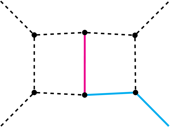
(b) planar no. 2

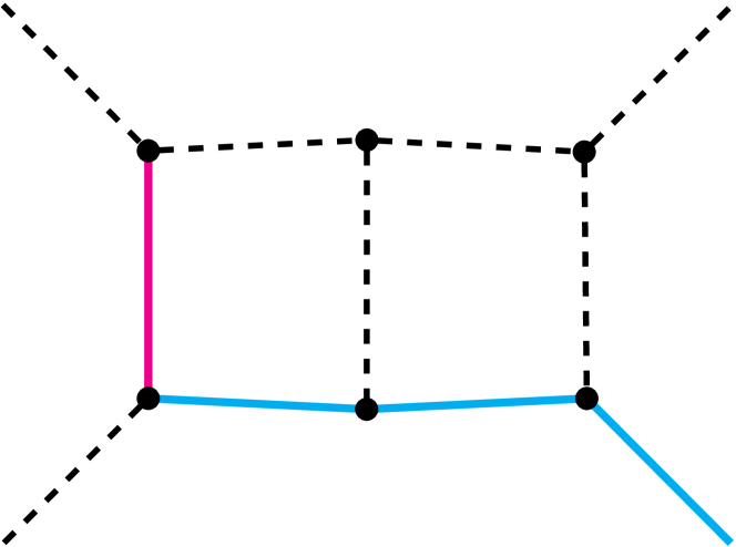
(c) planar no. 3

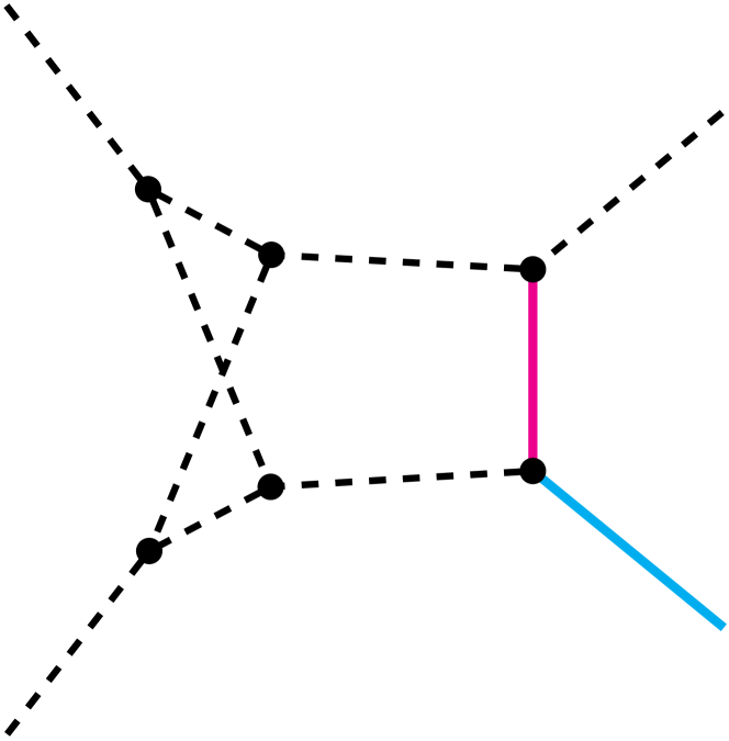
(d) non-planar no. 1

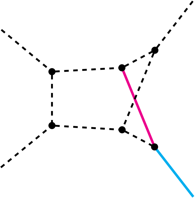
(e) non-planar no. 2

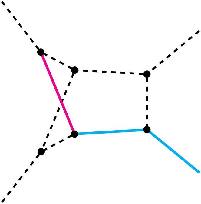
(f) non-planar no. 3

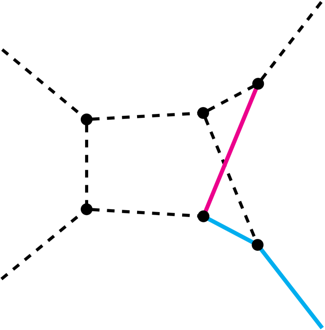
(g) non-planar no. 4

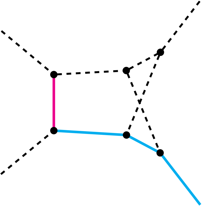
(h) non-planar no. 5

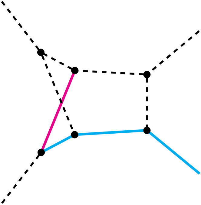
(i) non-planar no. 6

Figure 4: Topologies of integral families. Solid and dashed lines correspond to massive and massless particles respectively. Blue lines have mass $m_{t}$ while red lines have mass $m_{W}$. All families can be crossed ($p_{1}\leftrightarrow-p_{3}$) giving a total of 18 topologies.

The calculation of the master integrals needed to compute the non-factorisable corrections to single-top production is complicated as they depend on Mandelstam variables and on two masses, $m_{W}$ and $m_{t}$. We believe that, currently, their analytic computation is not possible. For this reason, we employ the auxiliary mass flow method Liu:2017jxz ; Liu:2020kpc ; Liu:2021wks to calculate them. To this end, we first construct a system of differential equations with respect to $m_{W}^{2}$, solve it starting from the boundary conditions at $m_{W}^{2}\to-i\infty$ as required by the causality prescription, and move to the physical value $m_{W}=80.379\text{~{}GeV}$. To do so, we require boundary conditions at $m_{W}^{2}\to-i\infty$. Although many integrals in this limit can be computed, we find that some of the boundary integrals are either hard to calculate analytically or that analytic results available in the literature are not known to sufficiently high orders in the $\epsilon$-expansion. Examples of such integrals are shown in Figure 5. We take a pragmatic approach and calculate these integrals numerically. Having already taken the limit $m_{W}^{2}\to-i\infty$, we analytically continue $m_{t}^{2}$ in internal propagators to the complex plane, as the causality prescriptions differ for internal and external masses. We proceed as follows. First, we rename the top mass $m_{t}$ that appears in internal propagators to $m$ and construct a system of differential equations with respect to $m^{2}$. We solve these equations starting at the boundary $m^{2}\to-i\infty$ and moving to the physical value $m=m_{t}=173\text{~{}GeV}$. We then use these results as boundary conditions for differential equations with respect to $m_{W}^{2}$ at $m_{W}^{2}=-i\infty$. The integrals shown in Figure 6 is the complete set that we used as boundary conditions either at $m_{W}^{2}=-i\infty$ or $m^{2}\to-i\infty$. We note that these integrals can be found in an ancillary file. In compiling this list, we have used results of Refs. tHooft:1978jhc ; Chetyrkin:1980pr ; Scharf:1993ds ; Gehrmann:1999as ; Gehrmann:2005pd . We have calculated two of the master integrals ($I_{16}$ and $I_{17}$ in Figure 6) since we could not find them in the literature.

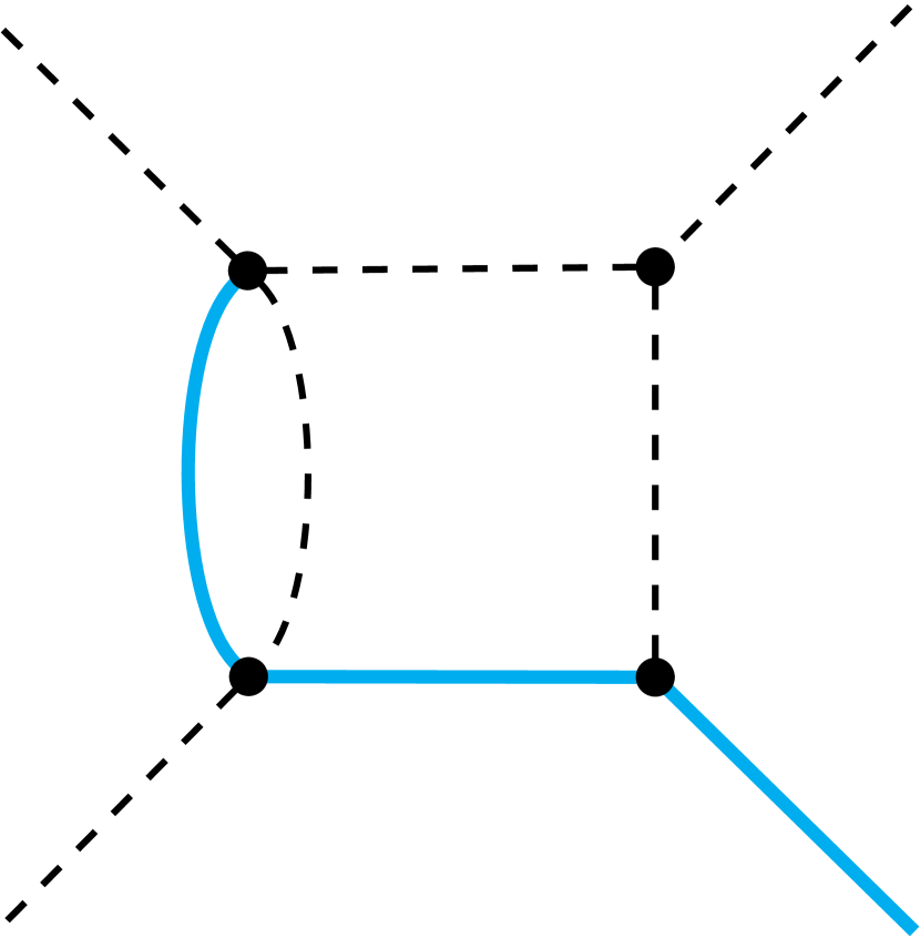
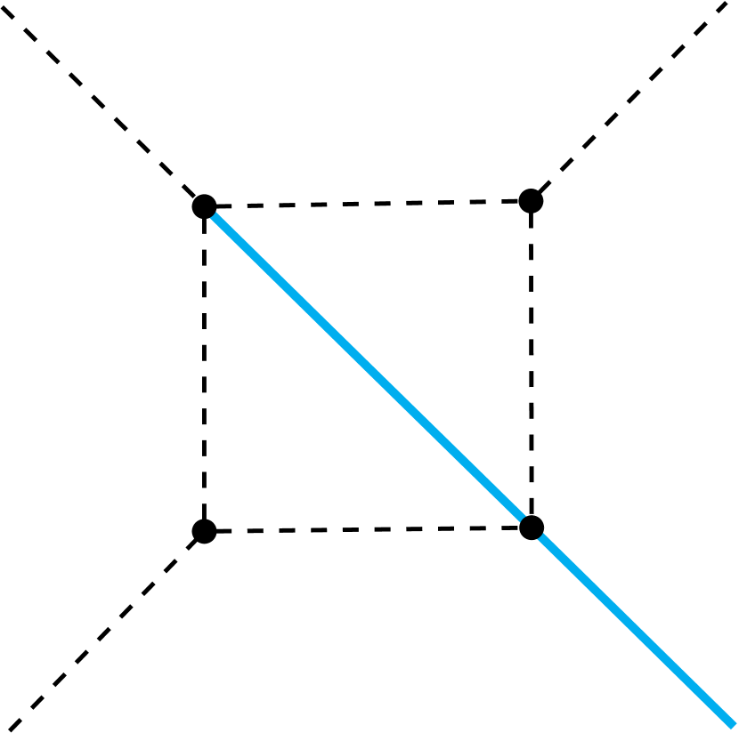
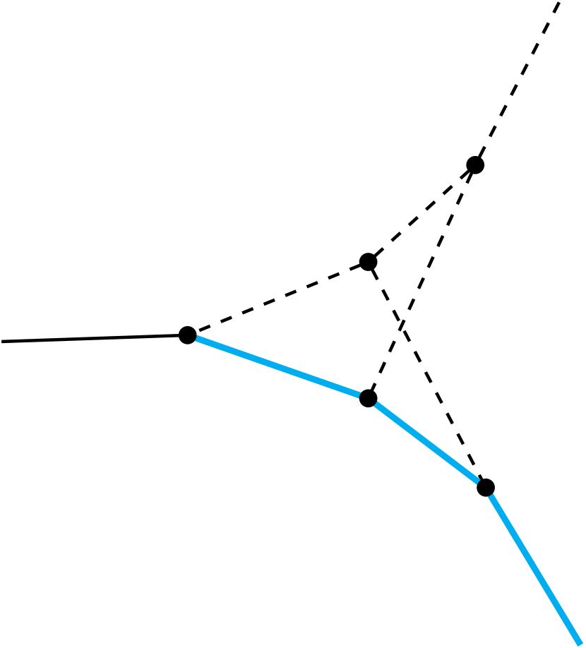
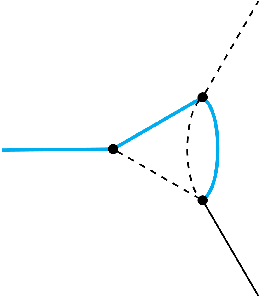
Figure 5: Examples of integrals that appear in the calculation of boundary conditions at $m_{W}^{2}\to-i\infty$. Solid and dashed lines correspond to massive and massless particles respectively. Blue lines have mass $m_{t}$ while black lines correspond to massive external particles.

(a) $I_{1}$

(b) $I_{2}$

(c) $I_{3}$

(d) $I_{4}$

(e) $I_{5}$

(f) $I_{6}$

(g) $I_{7}$

(h) $I_{8}$

(i) $I_{9}$

(j) $I_{10}$

(k) $I_{11}$

(l) $I_{12}$

(m) $I_{13}$

(n) $I_{14}$

(o) $I_{15}$

(p) $I_{16}$

(q) $I_{17}$

Figure 6: Master integrals for the boundary conditions. Solid and dashed lines correspond to massive and massless particles respectively. Thick solid lines represent particles with either mass $m$ or $m_{t}$ depending on whether the line is external or internal. If in some integrals thick solid lines appear both as external and internal, the mass is $m_{t}$. Thin solid lines correspond to external particles with the momentum squared $q^{2}$ where in general $q$ is a linear combination of external momenta $p_{1,2,3}$.

For phenomenology, we need to compute master integrals for many kinematic points relevant for the description of the process $u+b\to d+t$. To do that, we can simply solve the differential equations with respect to $m_{W}^{2}$ starting at $m_{W}^{2}=-i\infty$ for each pair of Mandelstam variables $s$ and $t$. This is the approach used in the previous papers by two of the present authors Bronnum-Hansen:2020mzk ; Bronnum-Hansen:2021olh . Alternatively, we can compute master integrals at a few kinematic points by solving differential equations in $m_{W}^{2}$ and then use these points as boundary conditions for differential equations with respect to the kinematic invariants $s$ and $t$ to calculate master integrals at other phase-phase points. We note that a similar approach has already been used in the literature Maltoni:2018zvp ; Frellesvig:2019byn ; Abreu:2020jxa . In the current calculation, we first generate several reference points in the phase space by solving the $m_{W}^{2}$ equation. Then we solve the equations in $s$ or $t$ to move from one of the reference points to the point of interest.

In general there are singularities in differential equations with respect to Mandelstam invariants; some of these singularities may appear as curves in the physical phase space. We need to use the correct causality prescription to cross such curves to avoid ending up on the unphysical sheet of the Riemann surface. One virtue of the auxiliary mass flow method is that the negative imaginary part of the mass provides a correct way to cross singular curves involving that mass. Whenever we encounter such a singular curve, we can move to the complex mass plane using the corresponding equation, then solve the $s$ and $t$ equations, and finally move back to the physical value of the $W$ boson mass. Evaluating all 428 master integrals to a precision of twenty digits at a typical phase-space point takes less than half an hour on a single CPU core.

We perform two checks to verify the integrals computed using the method described above. First, we calculate the master integrals by directly integrating over Feynman parameters using the publicly available program pySecDec Borowka:2017idc ; Borowka:2018goh . We perform a comparison at a physical phase-space point, away from kinematic thresholds and find good agreement of our and pySecDec results for the majority of the master integrals. Unfortunately, for some master integrals required in this paper, in particular non-planar boxes, we were unable to produce meaningful results with pySecDec.

Second, we have also checked the self-consistency of the differential equations. Indeed, solving the differential equations in $s$ and $t$ variables to move from one phase-space point to the next should produce the same results as solving the $m_{W}^{2}$-equations and directly moving from $m_{W}^{2}=-i\infty$ to the phase-space point of interest. We have checked that for several points across the phase space, master integrals evaluated in these two different ways agree up to the target precision of twenty digits.

4 Divergences in non-factorisable contributions to the scattering amplitude

In this section we discuss the $\epsilon$-pole structure of non-factorisable contributions to the scattering amplitude for the process $u+b\to d+t$. In principle, divergences of scattering amplitudes at higher orders in perturbative QCD are very well understood, see e.g. Refs. Catani:1998bh ; Czakon:2014oma ; Becher:2009qa . However, since in this paper we only deal with non-factorisable contributions to the two-loop amplitude, the relevant pole structure turns out to be quite special and, in fact, simpler than the general case.

Indeed, the first point to appreciate is that there are no ultraviolet divergences in non-factorisable corrections that contribute to the interference of the two-loop amplitude and the tree-level amplitude in Eq. (11). Therefore, we only need to use a relation between the bare and renormalised $\overline{\text{MS}}$ QCD coupling to zeroth order in perturbative QCD. It reads

$$\alpha_{s}^{\rm bare}=\mu^{2\epsilon}S_{\epsilon}\alpha_{s},$$ (24)

where $S_{\epsilon}=(4\pi)^{-\epsilon}\exp(\epsilon\gamma_{E})$ and $\gamma_{E}\approx 0.57721$ is the Euler-Mascheroni constant. Starting with the expression for individual Feynman diagrams, where the bare coupling constant enters, and rewriting it using Eq. (24), we obtain the amplitude introduced in Eq. (3).

In general, after renormalisation, the only $\epsilon$-poles present in the amplitude ${\cal A}$ are of infrared origin. To extract them, we follow Refs. Catani:1998bh ; Czakon:2014oma ; Becher:2009qa . To this end, we interpret the full amplitude in Eq. (3) as a vector in colour space. This amplitude is divergent; if poles of this amplitude are removed using the ${\overline{\rm MS}}$ prescription, we obtain a finite amplitude $|\mathcal{F}\rangle$ that is also a vector in colour space. Similar to the original amplitude $|\mathcal{A}\rangle$, $|\mathcal{F}\rangle$ can also be expanded in powers of $\alpha_{s}$. We write

$$|\mathcal{A}\rangle=\boldsymbol{Z}|\mathcal{F}\rangle,$$ (25)

where $\boldsymbol{Z}$ is an operator that removes infrared poles from the amplitude $|\mathcal{A}\rangle$. This operator satisfies the renormalisation group equation

$$\mu\frac{\,d}{\,d\mu}\boldsymbol{Z}=-\boldsymbol{\Gamma}\boldsymbol{Z},$$ (26)

where $\boldsymbol{\Gamma}$ is the so-called anomalous dimension operator. It reads Aybat:2006mz ; Becher:2009kw ; Czakon:2009zw ; Mitov:2009sv ; Ferroglia:2009ii ; Mitov:2010xw

$$\begin{split}\boldsymbol{\Gamma}(\{p_{i}\},m_{t},\mu)=&\sum_{(i,j)}\frac{\boldsymbol{T}_{i}\cdot\boldsymbol{T}_{j}}{2}\gamma_{\text{cusp}}(\alpha_{s})L_{ij}+\sum_{(I,j)}\boldsymbol{T}_{I}\cdot\boldsymbol{T}_{j}\gamma_{\text{cusp}}(\alpha_{s})L_{Ij}^{(m)}\\ &-\sum_{(I,J)}\frac{1}{2}\boldsymbol{T}_{I}\cdot\boldsymbol{T}_{J}\gamma_{\text{cusp}}(\nu_{IJ},\alpha_{s})+\sum_{i}\gamma^{i}(\alpha_{s})+\sum_{I}\gamma^{I}\left(\alpha_{s}\right)\\ &+\sum_{(I,J,K)}if^{abc}T^{a}_{I}T^{b}_{J}T^{c}_{K}F_{I}\left(\nu_{IJ},\nu_{JK},\nu_{KI}\right)\\ &+\sum_{(I,J)}\sum_{k}if^{abc}T_{I}^{a}T^{b}_{J}T^{c}_{k}f_{2}\left(\nu_{IJ},\ln\left(\frac{-\sigma_{Jk}v_{J}\cdot p_{k}}{-\sigma_{Ik}v_{I}\cdot p_{k}}\right)\right)\,.\end{split}$$ (27)

Small-letter indices refer to massless external partons whereas capital-letter indices denote massive external partons Becher:2009kw . When indices in a sum are shown in parenthesis, as e.g. $(i,j)$, the summation should be restricted to distinct indices. Also, $L_{ij}=\ln\left(\mu^{2}/(-s_{ij})\right)$ and $L_{Ij}^{(m)}=\ln\left(m_{t}\mu/(-s_{Ij})\right)$. Furthermore, the kinematic invariants that appear in the above equation are defined as

$$s_{ij}=2\sigma_{ij}p_{i}\cdot p_{j}+i\varepsilon\,,$$ (28)

where $\sigma_{ij}=1$ if both $p_{i}$ and $p_{j}$ are incoming or outgoing and $\sigma_{ij}=-1$ otherwise. Quantities $\nu_{IJ}$ are cusp angles, $v_{I}$ are four-velocities and $\boldsymbol{T}_{i}$ are colour-charge operators of the corresponding partons.

The operator $\boldsymbol{\Gamma}$ in Eq. (27) describes infrared and collinear divergences of the full amplitude that includes both factorisable and non-factorisable terms. However, if we focus on non-factorisable contributions only, the expression for $\boldsymbol{\Gamma}$ can be simplified. Indeed, we note that the last two terms in Eq. (27) are not needed for predicting infrared poles of the non-factorisable amplitude $\mathcal{A}_{\rm nf}^{(2)}$ since they are proportional to non-abelian colour factors. As we have explained in Section 2, non-abelian colour factors cannot arise in the contributions that we are interested in. Furthermore, the two sums over the anomalous dimensions $\gamma^{(i)}$ and $\gamma^{(I)}$ cannot contribute to $\mathcal{A}_{\rm nf}^{(2)}$ either since they are related to collinear emissions that, in physical gauges, should be associated with factorisable parts of the amplitude.

We are left with three sums that involve products of two colour-charge operators in Eq. (27). In our case, there are three massless and one massive external particle; hence, the third sum in Eq. (27) that should be performed over two distinct massive indices is not relevant for us and can be discarded. Moreover, the non-factorisable contributions involve gluon exchanges between different fermion lines. Hence only four products of colour-charge operators contribute; they are $\boldsymbol{T}_{1}\cdot\boldsymbol{T}_{2}$, $\boldsymbol{T}_{1}\cdot\boldsymbol{T}_{4}$, $\boldsymbol{T}_{2}\cdot\boldsymbol{T}_{3}$, and $\boldsymbol{T}_{3}\cdot\boldsymbol{T}_{4}$. Finally, the cusp anomalous dimension is given by Becher:2009kw ; Becher:2009cu

$$\gamma_{\text{cusp}}=4\left(\frac{\alpha_{s}}{4\pi}\right)+\left[\left(\frac{268}{9}-\frac{4\pi^{2}}{3}\right)C_{A}-\frac{80}{9}T_{F}n_{l}\right]\left(\frac{\alpha_{s}}{4\pi}\right)^{2}+\mathcal{O}(\alpha_{s}^{3})\,.$$ (29)

We note that the ${\cal O}(\alpha_{s}^{2})$ contribution to $\gamma_{\text{cusp}}$ contains terms that are either proportional to a non-abelian colour factor $C_{A}$ or to the number of light fermions $n_{f}$ and none of these parameters appear in the non-factorisable diagrams. Hence, if we are interested in non-factorisable corrections only, the $C_{A}$- and $n_{f}$-dependent contributions to $\gamma_{\text{cusp}}$ should be discarded. Therefore, we are allowed to replace

$$\gamma_{\text{cusp}}\to\gamma_{\rm nf}=4\left(\frac{\alpha_{s}}{4\pi}\right),$$ (30)

in the expression for $\boldsymbol{\Gamma}$ in Eq. (27).

We define the part of the operator $\boldsymbol{\Gamma}$ that is relevant for non-factorisable corrections as $\boldsymbol{\Gamma}_{\rm nf}$. As a consequence of the above discussion, it reads

$$\boldsymbol{\Gamma}_{\rm nf}(\{p_{i}\},m_{t},\mu) =\left(\frac{\alpha_{s}}{4\pi}\right)\boldsymbol{\Gamma}_{0,\rm nf}(\{p_{i}\},m_{t},\mu),$$ (31)

where

$$\boldsymbol{\Gamma}_{0,\rm nf} =4\bigg{[}\boldsymbol{T}_{1}\cdot\boldsymbol{T}_{2}\ln\left(\frac{\mu^{2}}{-s-i\varepsilon}\right)+\boldsymbol{T}_{2}\cdot\boldsymbol{T}_{3}\ln\left(\frac{\mu^{2}}{-u-i\varepsilon}\right)$$ (32)

$$\quad+\boldsymbol{T}_{1}\cdot\boldsymbol{T}_{4}\ln\left(\frac{\mu\>m_{t}}{m_{t}^{2}-u-i\varepsilon}\right)+\boldsymbol{T}_{3}\cdot\boldsymbol{T}_{4}\ln\left(\frac{\mu\>m_{t}}{m_{t}^{2}-s-i\varepsilon}\right)\bigg{]}.$$ (33)

We can solve Eq. (26) with $\boldsymbol{\Gamma}_{\rm nf}$ in place of $\boldsymbol{\Gamma}$ order by order in $\alpha_{s}$, to determine the operator $\boldsymbol{Z}_{\rm nf}$; we assume that $\boldsymbol{Z}_{\rm nf}=1+{\cal O}(\alpha_{s})$. This solution is much simpler than the one for the full amplitude since perturbative running of the coupling constant cannot play a role in the non-factorisable contribution through ${\cal O}(\alpha_{s}^{2})$. As the result, we find a remarkably simple expression

$$\boldsymbol{Z}_{\rm nf}=1+\left(\frac{\alpha_{s}}{4\pi}\right)\frac{\boldsymbol{\Gamma}_{0,\rm nf}}{2\epsilon}+\left(\frac{\alpha_{s}}{4\pi}\right)^{2}\frac{{\boldsymbol{\Gamma}_{0,\rm nf}}^{2}}{8\epsilon^{2}}+{\cal O}(\alpha_{s}^{3}),$$ (34)

which emphasizes that through two loops non-factorisable contributions are abelian even if computed in a non-abelian theory like QCD. We also note that in comparison to infrared $\epsilon$-poles in the full amplitude, divergences in non-factorisable contributions are much more mild and start at $1/\epsilon$ at ${\cal O}(\alpha_{s})$ and at $1/\epsilon^{2}$ at ${\cal O}(\alpha_{s}^{2})$. This is a direct consequence of the fact that collinear divergences cannot appear in a non-factorisable amplitude due to its very definition. Hence, all infrared poles present in Eq. (34) are of soft origin.

It is now straightforward to predict $\epsilon$-poles in non-factorisable contributions to cross sections. We find

$$\begin{split}\langle\mathcal{A}^{(0)}|\mathcal{A}_{\rm nf}^{(2)}\rangle&=-\frac{1}{8\epsilon^{2}}\langle\mathcal{A}^{(0)}|\boldsymbol{\Gamma}_{0,\rm nf}^{2}|\mathcal{A}^{(0)}\rangle+\frac{1}{2\epsilon}\langle\mathcal{A}^{(0)}|\boldsymbol{\Gamma}_{0,\rm nf}|\mathcal{A}_{\rm nf}^{(1)}\rangle+\langle\mathcal{A}^{(0)}|\mathcal{F}_{\rm nf}^{(2)}\rangle,\\ \langle\mathcal{A}_{\rm nf}^{(1)}|\mathcal{A}_{\rm nf}^{(1)}\rangle&=\frac{1}{4\epsilon^{2}}\langle\mathcal{A}^{(0)}||\boldsymbol{\Gamma}_{0,\rm nf}|^{2}|\mathcal{A}^{(0)}\rangle+\frac{1}{2\epsilon}\langle\mathcal{A}_{\rm nf}^{(1)}|\boldsymbol{\Gamma}_{0,\rm nf}|\mathcal{A}^{(0)}\rangle\\ &\;\;\;\;\;\;\;\;\;\;\;\;\;\;\;\;\;\;\;\;\;\;\;\;\;\;\;\;\;+\frac{1}{2\epsilon}\langle\mathcal{A}^{(0)}|\boldsymbol{\Gamma}_{0,\rm nf}^{\dagger}|\mathcal{A}_{\rm nf}^{(1)}\rangle+\langle\mathcal{F}_{\rm nf}^{(1)}|\mathcal{F}_{\rm nf}^{(1)}\rangle.\end{split}$$ (35)

We can easily calculate matrix elements of the relevant colour-charge operators. As an example, consider $\langle\mathcal{A}^{(0)}|\boldsymbol{\Gamma}_{0,\rm nf}^{2}|\mathcal{A}^{(0)}\rangle$. The action of colour-charge operators on vectors in the colour space is defined as follows

$$\langle\boldsymbol{e}|\boldsymbol{T}_{i}^{a}|\boldsymbol{d}\rangle=T_{e_{i}d_{i}}^{a}\prod_{j\neq i}\delta_{e_{j}d_{j}},\quad T_{e_{i}d_{i}}^{a}=\begin{cases}t_{e_{i}d_{i}}^{a}&\text{final state quark},\\ -t_{d_{i}e_{i}}^{a}&\text{initial state quark}.\end{cases}\,.$$ (36)

In the above equation $|\boldsymbol{d}\rangle$ and $|\boldsymbol{e}\rangle$ are vectors in colour space and the $SU(3)$ generators $t^{a,b}$ are normalised in a standard way

$$\text{Tr}\left(t^{a}t^{b}\right)=\frac{1}{2}\delta_{ab}\,.$$ (37)

Using these definitions, it is easy to see that for all combinations of colour-charge operators that appear in $\boldsymbol{\Gamma}_{0,\rm nf}^{2}$ the following results holds

$$\langle\mathcal{A}^{(0)}|(\boldsymbol{T}_{i}\boldsymbol{T}_{j})(\boldsymbol{T}_{k}\boldsymbol{T}_{m})|\mathcal{A}^{(0)}\rangle=(-1)^{n_{i}}\frac{N_{c}^{2}-1}{4}\,.$$ (38)

Here $n_{i}$ is the number of indices among $i,j,k,m$ that correspond to initial-state partons. Hence, we find

$$\langle\mathcal{A}^{(0)}|\boldsymbol{\Gamma}_{0,\rm nf}^{2}|\mathcal{A}^{(0)}\rangle=4(N_{c}^{2}-1)|A^{(0)}|^{2}\left(\ln\left(\frac{-u-i\varepsilon}{-s-i\varepsilon}\right)+\ln\left(\frac{m_{t}^{2}-u-i\varepsilon}{m_{t}^{2}-s-i\varepsilon}\right)\right)^{2}.$$ (39)

All other contributions that appear in Eq. (35) can be computed in a similar way.

Predictions for infrared poles of the two-loop non-factorisable contribution to the cross section provide an important cross check of the correctness of the calculation. As an example of the level of numerical precision that we have achieved for the $\epsilon$-poles of the two-loop non-factorisable amplitude, in Table 2 we compare the results of the evaluation of $\langle\mathcal{A}^{(0)}|\mathcal{A}_{\rm nf}^{(2)}\rangle$ with the analytic predictions for its $\epsilon$-poles. We observe that analytic and numerical results for $\epsilon$-poles agree to 15 digits. We also find that the $\epsilon$-poles of $\langle\mathcal{A}_{\rm nf}^{(1)}|\mathcal{A}_{\rm nf}^{(1)}\rangle$ are accurate to about 30 digits throughout the phase space since the one-loop integrals are evaluated to that precision. In Appendix A we provide additional numerical results for non-factorizable contributions, including their finite parts, for further reference.

	$\epsilon^{-2}$	$\epsilon^{-1}$
$\langle\mathcal{A}^{(0)}|\mathcal{A}_{\rm nf}^{(2)}\rangle$	$-229.0940408654660-8.978163333241640i$	$-301.1802988944764-264.1773596529505i$
IR poles	$-229.0940408654665-8.978163333241973i$	$-301.1802988944791-264.1773596529535i$

Table 2: Computed and predicted $\epsilon$-poles for a typical phase space point. We use $s\approx 104337~{}\text{GeV}^{2}$ and $t\approx-5179.68~{}\text{GeV}^{2}$ for a comparison.

5 Results

Having computed the two-loop non-factorisable contribution to the scattering amplitude for single-top production, we can study its impact on the single-top production cross section. Such an analysis is necessarily incomplete. Indeed, since in this paper we restrict ourselves to virtual corrections, we will have to consider quantities that depend on how the infrared singularities are removed. To arrive at the physical result which is independent of the infrared regulator, we need to combine virtual corrections computed in this paper with real-emission non-factorisable contributions. We intend to do this in the future. However, we believe it is still useful to study the contribution of virtual corrections computed in this paper to the single-top production cross section. Indeed, as we explained in the previous sections, we computed master integrals numerically. Hence, it is important to show that our numerical evaluation is sufficiently fast and robust to enable realistic phenomenological studies.

To address this point, we study non-factorisable corrections to the differential cross section for single-top production at the LHC in the $ub$-channel. We write

$$\,d\sigma^{ub}_{pp\rightarrow d+t}=\sum_{\begin{subarray}{c}i,j=u,b\\ i\neq j\end{subarray}}\int\,dx_{1}\,dx_{2}\,f_{i}(x_{1})f_{j}(x_{2})\,d\hat{\sigma}_{ij\rightarrow d+t}(x_{1},x_{2})\,,$$ (40)

where $f_{i}$ are parton distribution functions (PDFs) and the superscript indicates that we only consider the $ub$ initial state. We consider proton-proton collision at 13 TeV and use the NNPDF31_lo_as_0118 parton distribution functions Buckley:2014ana ; NNPDF:2017mvq . The renormalisation and factorisation scales are fixed at $\mu=m_{t}$. The value of the strong coupling constant $\alpha_{s}$ is provided by the PDF sets. We use $m_{t}=173~{}{\rm GeV}$, $m_{W}=80.379~{}{\rm GeV}$, the Fermi constant $G_{F}=1.16637\times 10^{-5}~{}~{}{\rm GeV}^{-2}$ and set CKM matrix elements to one. Finally, we note that no kinematic cuts are applied.

We compute the partonic cross section using the finite amplitude ${\mathcal{F}}$. We write

$$\hat{\sigma}_{ij\rightarrow d+t}=\frac{1}{8N_{c}^{2}\>s}\int\frac{\,d^{3}p_{3}}{(2\pi)^{3}\>2E_{3}}\frac{\,d^{3}p_{4}}{(2\pi)^{3}\>2E_{4}}{\langle\mathcal{F}|\mathcal{F}\rangle}\>(2\pi)^{4}\delta^{(4)}\left(p_{1}+p_{2}-p_{3}-p_{4}\right)\,,$$ (41)

where the prefactor on the right-hand side includes spin- and colour-averaging factors. Since we are interested in the non-factorisable two-loop QCD contribution we use

$$\langle\mathcal{F}|\mathcal{F}\rangle=\langle\mathcal{F}^{(0)}|\mathcal{F}^{(0)}\rangle+\left(\frac{\alpha_{s}}{4\pi}\right)^{2}\left[\langle\mathcal{F}_{\rm nf}^{(1)}|\mathcal{F}_{\rm nf}^{(1)}\rangle+2\Re\left\{\langle\mathcal{F}^{(0)}|\mathcal{F}_{\rm nf}^{(2)}\rangle\right\}\right]\,.$$ (42)

As we already mentioned, ${\cal O}(\alpha_{s})$ non-factorisable contribution vanishes due to colour conservation.

In practice, the evaluation of the non-factorisable contribution to the cross section proceeds as follows. As a first step we produce a reliable grid for the evaluation of the leading order cross section as well as top rapidity and $p_{\perp}$ distributions. Once the grid is obtained, we randomly draw kinematic points from it, compute $\langle\mathcal{F}|\mathcal{F}\rangle$ and the phase-space weight for these points and obtain an estimate of the cross section including non-factorisable corrections.

We find the following result

$$\sigma^{ub}_{pp\to dt}=\left(90.3+0.3\left(\frac{\alpha_{s}(\mu_{\rm nf})}{0.108}\right)^{2}\right)~{}{\rm pb},$$ (43)

where the first term is the leading order cross section and the second term is the non-factorisable NNLO contribution. We have indicated in Eq. (43) that one can change the scale of the strong coupling constant in non-factorisable corrections independently of the rest of the calculation. This is so because the non-factorisable corrections appear for the first time at NNLO so that they cannot compensate the scale variations of leading and next-to-leading order cross sections. This remark is important as the choice of $\mu_{\rm nf}$ in Eq. (43) has obvious consequences for how large these corrections actually are. We note that the non-factorisable correction $0.3~{}{\rm pb}$ in Eq. (43) is the result of the cancellation between the one-loop squared contribution ($0.7$ pb) and the interference of the two-loop amplitude with the leading order one ($-0.4$ pb).

It follows from Eq. (43) that non-factorisable corrections are quite small; they change the leading order cross section by $0.3$ percent. However, in spite of being small they are actually of the same order as the factorisable corrections to single-top production. Indeed, factorisable corrections are supposed to be the dominant ones but they change the NLO single-top production cross section by less than a percent (see e.g. Ref. Campbell:2020fhf ). Moreover, as we already mentioned, the appropriate choice of the scale $\mu_{\rm nf}$ in Eq. (43) is unclear at present. However, since these corrections always involve exchanges between two quark lines, it is reasonable to assume that proper $\mu_{\rm nf}$ should be related to a typical transverse momentum of the top quark in single-top production, which is about $40-60~{}{\rm GeV}$. If so, the magnitude of the non-factorisable correction will increase by a factor ${\cal O}(1.5)$ and become close to half a percent.

Having discussed the total cross section we move to kinematic distributions. We begin with the distribution of the top quark transverse momentum; it is shown in Figure 7. In the upper pane we display the differential cross section at leading order and including non-factorisable corrections. In the lower pane, we show ratios of the NNLO non-factorisable correction to the leading order differential cross section as a function of the top quark transverse momentum.

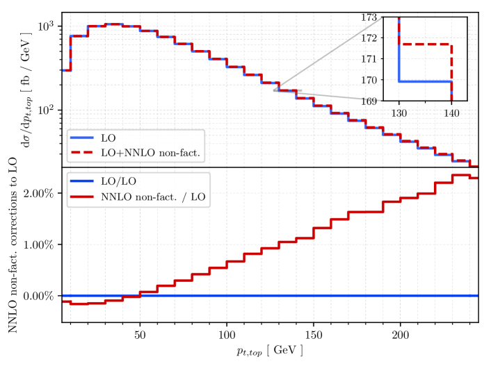
Figure 7: The top-quark transverse momentum distribution. In the upper pane, the blue line corresponds to the leading order distribution whereas the dashed, red line to the distribution with NNLO QCD non-factorisable corrections included. In the lower pane, the ratio of non-factorisable corrections to the leading order distribution is presented. See text for further details.

It follows from Figure 7 that non-factorisable corrections exhibit significant $p_{\perp}$-dependence. Indeed, they are quite small and negative for $p_{\perp}$ between $0$ and $50$ GeV. For larger $p_{\perp}$, they start growing and reach ${\cal O}(1\%)$ at $p_{\perp}\sim 100~{}{\rm GeV}$. It is interesting to note that the NNLO factorisable correction exhibits a similar $p_{\perp}$-dependence Brucherseifer:2014ama ; Berger:2016oht ; Campbell:2020fhf which means that the relative importance of factorisable and non-factorisable corrections remains constant across the phase space.

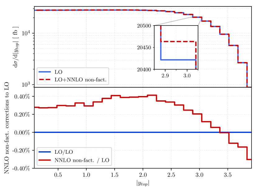
(a) The top-quark rapidity distribution.

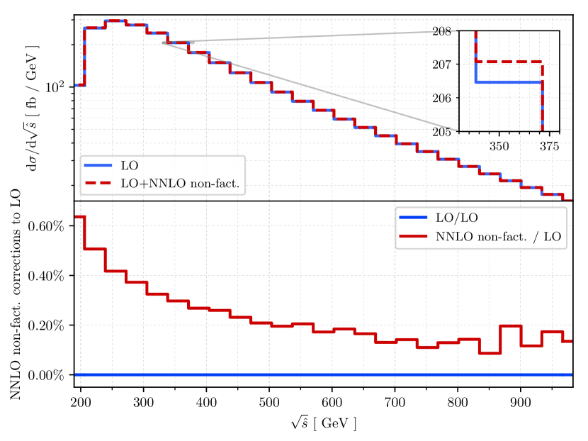
(b) Differential cross section with respect to the partonic invariant energy $\sqrt{\hat{s}}$.

Figure 8: Distributions of the absolute value of the top-quark rapidity (left) and the partonic center of mass energy $\sqrt{\hat{s}}$ (right). Upper panes show leading order distributions as well as distributions with non-factorisable corrections included. Lower panes show the ratio of non-factorisable corrections to leading order distributions. See text for further details.

In Figure 8, we show the impact of non-factorisable corrections on the top-quark rapidity distribution and on the distribution of the invariant mass of the top quark and the light-quark jet which for a $2\to 2$ process is equivalent to the partonic centre-of-mass energy $\sqrt{\hat{s}}$. It follows from Figure 8(a) that non-factorisable corrections to the rapidity distributions are ${\cal O}(0.3\%)$ for $|y_{t}|<2.5$; for larger rapidities corrections quickly become negative. The non-factorisable corrections to the $\sqrt{\hat{s}}$ distribution shown in Figure 8(b) are positive and change from ${\cal O}(0.6\%)$ at the threshold to ${\cal O}(0.1\%)$ at large partonic centre-of-mass energies.

6 Conclusions

In this paper, we computed the contribution of two-loop non-factorisable virtual corrections to $t$-channel single-top production cross section. This is the last missing part of the two-loop amplitude needed for a complete description of this process through NNLO QCD. Exact dependence on the top quark mass is retained throughout the calculation.

The calculation reported in this paper involves numerical computation of master integrals using the auxiliary mass flow method Liu:2017jxz ; Liu:2020kpc ; Liu:2021wks . For this reason it is important to demonstrate that the calculation is sufficiently robust and can be used to produce results relevant for phenomenology. We have shown this by studying the impact of finite remainders of non-factorisable virtual corrections on the single-top production cross section and basic kinematic distributions. We have found that non-factorisable corrections are smaller than, but quite comparable to, the factorisable ones, especially since it is not very clear which scale for the strong coupling constant should be used when computing them.

We emphasize that phenomenological studies reported in Section 5 are necessarily incomplete since they include only virtual non-factorisable corrections. As we explained in Section 4, these virtual corrections are infrared divergent; hence, to arrive at physical predictions, we also require non-factorisable real-emission contributions. Given the recent progress with understanding of how fully-differential NNLO QCD computations can be performed, we believe that it is straightforward to compute the non-factorisable real-emission corrections to single-top production; we plan to do this in the near future. Finally, realistic phenomenological studies require an inclusion of top quark decays. Since we computed non-factorisable contributions to two-loop helicity amplitudes, it is straightforward to accommodate top quark decays into our computation as well.

Appendix A Numerical evaluations

In Table 3 we provide numerical results for the non-factorisable contribution to the two-loop amplitude for three kinematic points.

$\langle\mathcal{A}^{(0)}|\mathcal{A}_{\rm nf}^{(2)}\rangle(s,t)$	$\epsilon^{-2}$	$\epsilon^{-1}$	$\epsilon^{0}$
$(104337.30,-5179.6797)$	$-229.09404-8.9781633i$	$-301.18030-264.17736i$	$380.61217+307.59053i$
$(51824.679,-16060.887)$	$-8.2985887-4.8234599i$	$-7.2779624-22.421862i$	$42.503179+59.484685i$
$(2728123.9,-69809.245)$	$-5061.2720-83.997993i$	$34392.588-1255.7061i$	$-1507.7598+18782.966i$

Table 3: Numerical results for non-factorisable corrections at three different kinematic points specified by $(s,t)$ in units of $\text{GeV}^{2}$. For presentation purposes we have truncated numerical values to eight digits. We use $m_{W}=80.379~{}{\rm GeV}$, $m_{t}=173~{}{\rm GeV}$ and $\mu=m_{t}$. See main text for further details.

References

- (1) A. Giammanco and R. Schwienhorst, Single top-quark production at the Tevatron and the LHC, Rev. Mod. Phys. 90 (2018) 035001 [1710.10699].
- (2) ATLAS collaboration, Probing the W tb vertex structure in t-channel single-top-quark production and decay in pp collisions at TeV with the ATLAS detector, JHEP 04 (2017) 124 [1702.08309].
- (3) ATLAS, CMS collaboration, Combinations of single-top-quark production cross-section measurements and |fLVVtb| determinations at = 7 and 8 TeV with the ATLAS and CMS experiments, JHEP 05 (2019) 088 [1902.07158].
- (4) CMS collaboration, Measurement of CKM matrix elements in single top quark -channel production in proton-proton collisions at 13 TeV, Phys. Lett. B 808 (2020) 135609 [2004.12181].
- (5) CMS collaboration, Measurement of the ratio in pp collisions at = 8 TeV, Phys. Lett. B 736 (2014) 33 [1404.2292].
- (6) CMS collaboration, Measurement of the top quark mass using single top quark events in proton-proton collisions at TeV, Eur. Phys. J. C 77 (2017) 354 [1703.02530].
- (7) CMS collaboration, Measurement of differential cross sections and charge ratios for t-channel single top quark production in proton–proton collisions at , Eur. Phys. J. C 80 (2020) 370 [1907.08330].
- (8) ATLAS collaboration, Fiducial, total and differential cross-section measurements of -channel single top-quark production in collisions at 8 TeV using data collected by the ATLAS detector, Eur. Phys. J. C 77 (2017) 531 [1702.02859].
- (9) B.W. Harris, E. Laenen, L. Phaf, Z. Sullivan and S. Weinzierl, The Fully Differential Single Top Quark Cross-Section in Next to Leading Order QCD, Phys. Rev. D 66 (2002) 054024 [hep-ph/0207055].
- (10) J.M. Campbell, R.K. Ellis and F. Tramontano, Single top production and decay at next-to-leading order, Phys. Rev. D 70 (2004) 094012 [hep-ph/0408158].
- (11) Z. Sullivan, Understanding single-top-quark production and jets at hadron colliders, Phys. Rev. D 70 (2004) 114012 [hep-ph/0408049].
- (12) Q.-H. Cao and C.P. Yuan, Single top quark production and decay at next-to-leading order in hadron collision, Phys. Rev. D 71 (2005) 054022 [hep-ph/0408180].
- (13) R. Schwienhorst, C.P. Yuan, C. Mueller and Q.-H. Cao, Single top quark production and decay in the -channel at next-to-leading order at the LHC, Phys. Rev. D 83 (2011) 034019 [1012.5132].
- (14) M. Gao and J. Gao, Differential distributions for Single Top Quark Production at the LHeC, 2103.15846.
- (15) M. Brucherseifer, F. Caola and K. Melnikov, On the NNLO QCD corrections to single-top production at the LHC, Phys. Lett. B 736 (2014) 58 [1404.7116].
- (16) E.L. Berger, J. Gao, C.P. Yuan and H.X. Zhu, NNLO QCD Corrections to t-channel Single Top-Quark Production and Decay, Phys. Rev. D 94 (2016) 071501 [1606.08463].
- (17) J. Campbell, T. Neumann and Z. Sullivan, Single-top-quark production in the -channel at NNLO, JHEP 02 (2021) 040 [2012.01574].
- (18) R.J. Glauber, Lectures in Theoretical Physics, Wiley-Interscience, New York (1959).
- (19) T. Liu, K. Melnikov and A.A. Penin, Nonfactorizable QCD Effects in Higgs Boson Production via Vector Boson Fusion, Phys. Rev. Lett. 123 (2019) 122002 [1906.10899].
- (20) X. Liu, Y.-Q. Ma and C.-Y. Wang, A Systematic and Efficient Method to Compute Multi-loop Master Integrals, Phys. Lett. B 779 (2018) 353 [1711.09572].
- (21) X. Liu, Y.-Q. Ma, W. Tao and P. Zhang, Calculation of Feynman loop integration and phase-space integration via auxiliary mass flow, Chin. Phys. C 45 (2021) 013115 [2009.07987].
- (22) X. Liu and Y.-Q. Ma, Multiloop corrections for collider processes using auxiliary mass flow, 2107.01864.
- (23) M. Assadsolimani, P. Kant, B. Tausk and P. Uwer, Calculation of two-loop QCD corrections for hadronic single top-quark production in the channel, Phys. Rev. D 90 (2014) 114024 [1409.3654].
- (24) N.u. Basat, Z. Li and Y. Wang, Reduction of planar double-box diagram for single-top production via auxiliary mass flow, 2102.08225.
- (25) C. Brønnum-Hansen and C.-Y. Wang, Contribution of third generation quarks to two-loop helicity amplitudes for W boson pair production in gluon fusion, JHEP 01 (2021) 170 [2009.03742].
- (26) C. Brønnum-Hansen and C.-Y. Wang, Top quark contribution to two-loop helicity amplitudes for boson pair production in gluon fusion, JHEP 05 (2021) 244 [2101.12095].
- (27) R.J. Gonsalves, DIMENSIONALLY REGULARIZED TWO LOOP ON-SHELL QUARK FORM-FACTOR, Phys. Rev. D 28 (1983) 1542.
- (28) W.L. van Neerven, Dimensional Regularization of Mass and Infrared Singularities in Two Loop On-shell Vertex Functions, Nucl. Phys. B 268 (1986) 453.
- (29) R. Bonciani and A. Ferroglia, Two-Loop QCD Corrections to the Heavy-to-Light Quark Decay, JHEP 11 (2008) 065 [0809.4687].
- (30) G. Bell, NNLO corrections to inclusive semileptonic B decays in the shape-function region, Nucl. Phys. B 812 (2009) 264 [0810.5695].
- (31) H.M. Asatrian, C. Greub and B.D. Pecjak, NNLO corrections to anti-B — X(u) l anti-nu in the shape-function region, Phys. Rev. D 78 (2008) 114028 [0810.0987].
- (32) M. Beneke, T. Huber and X.Q. Li, Two-loop QCD correction to differential semi-leptonic b — u decays in the shape-function region, Nucl. Phys. B 811 (2009) 77 [0810.1230].
- (33) T. Huber, On a two-loop crossed six-line master integral with two massive lines, JHEP 03 (2009) 024 [0901.2133].
- (34) P. Nogueira, Automatic Feynman graph generation, J. Comput. Phys. 105 (1993) 279.
- (35) A. von Manteuffel and C. Studerus, Reduze 2 - Distributed Feynman Integral Reduction, 1201.4330.
- (36) J. Klappert, F. Lange, P. Maierhöfer and J. Usovitsch, Integral Reduction with Kira 2.0 and Finite Field Methods, 2008.06494.
- (37) G. ’t Hooft and M. Veltman, Scalar One Loop Integrals, Nucl. Phys. B 153 (1979) 365.
- (38) K. Chetyrkin, A. Kataev and F. Tkachov, New Approach to Evaluation of Multiloop Feynman Integrals: The Gegenbauer Polynomial x Space Technique, Nucl. Phys. B 174 (1980) 345.
- (39) R. Scharf and J. Tausk, Scalar two loop integrals for gauge boson selfenergy diagrams with a massless fermion loop, Nucl. Phys. B 412 (1994) 523.
- (40) T. Gehrmann and E. Remiddi, Differential equations for two loop four point functions, Nucl. Phys. B 580 (2000) 485 [hep-ph/9912329].
- (41) T. Gehrmann, T. Huber and D. Maitre, Two-loop quark and gluon form-factors in dimensional regularisation, Phys. Lett. B 622 (2005) 295 [hep-ph/0507061].
- (42) F. Maltoni, M.K. Mandal and X. Zhao, Top-quark effects in diphoton production through gluon fusion at next-to-leading order in QCD, Phys. Rev. D 100 (2019) 071501 [1812.08703].
- (43) H. Frellesvig, M. Hidding, L. Maestri, F. Moriello and G. Salvatori, The complete set of two-loop master integrals for Higgs + jet production in QCD, JHEP 06 (2020) 093 [1911.06308].
- (44) S. Abreu, H. Ita, F. Moriello, B. Page, W. Tschernow and M. Zeng, Two-Loop Integrals for Planar Five-Point One-Mass Processes, JHEP 11 (2020) 117 [2005.04195].
- (45) S. Borowka, G. Heinrich, S. Jahn, S. Jones, M. Kerner, J. Schlenk et al., pySecDec: a toolbox for the numerical evaluation of multi-scale integrals, Comput. Phys. Commun. 222 (2018) 313 [1703.09692].
- (46) S. Borowka, G. Heinrich, S. Jahn, S. Jones, M. Kerner and J. Schlenk, A GPU compatible quasi-Monte Carlo integrator interfaced to pySecDec, Comput. Phys. Commun. 240 (2019) 120 [1811.11720].
- (47) S. Catani, The Singular behavior of QCD amplitudes at two loop order, Phys. Lett. B 427 (1998) 161 [hep-ph/9802439].
- (48) M. Czakon and D. Heymes, Four-dimensional formulation of the sector-improved residue subtraction scheme, Nucl. Phys. B 890 (2014) 152 [1408.2500].
- (49) T. Becher and M. Neubert, On the Structure of Infrared Singularities of Gauge-Theory Amplitudes, JHEP 06 (2009) 081 [0903.1126].
- (50) S.M. Aybat, L.J. Dixon and G.F. Sterman, The Two-loop soft anomalous dimension matrix and resummation at next-to-next-to leading pole, Phys. Rev. D 74 (2006) 074004 [hep-ph/0607309].
- (51) T. Becher and M. Neubert, Infrared singularities of QCD amplitudes with massive partons, Phys. Rev. D 79 (2009) 125004 [0904.1021].
- (52) M. Czakon, A. Mitov and G.F. Sterman, Threshold Resummation for Top-Pair Hadroproduction to Next-to-Next-to-Leading Log, Phys. Rev. D 80 (2009) 074017 [0907.1790].
- (53) A. Mitov, G.F. Sterman and I. Sung, The Massive Soft Anomalous Dimension Matrix at Two Loops, Phys. Rev. D 79 (2009) 094015 [0903.3241].
- (54) A. Ferroglia, M. Neubert, B.D. Pecjak and L.L. Yang, Two-loop divergences of massive scattering amplitudes in non-abelian gauge theories, JHEP 11 (2009) 062 [0908.3676].
- (55) A. Mitov, G.F. Sterman and I. Sung, Computation of the Soft Anomalous Dimension Matrix in Coordinate Space, Phys. Rev. D 82 (2010) 034020 [1005.4646].
- (56) T. Becher and M. Neubert, Infrared singularities of scattering amplitudes in perturbative QCD, Phys. Rev. Lett. 102 (2009) 162001 [0901.0722].
- (57) A. Buckley, J. Ferrando, S. Lloyd, K. Nordström, B. Page, M. Rüfenacht et al., LHAPDF6: parton density access in the LHC precision era, Eur. Phys. J. C 75 (2015) 132 [1412.7420].
- (58) NNPDF collaboration, Parton distributions from high-precision collider data, Eur. Phys. J. C 77 (2017) 663 [1706.00428].
- (59) J. Alwall, R. Frederix, S. Frixione, V. Hirschi, F. Maltoni, O. Mattelaer et al., The automated computation of tree-level and next-to-leading order differential cross sections, and their matching to parton shower simulations, JHEP 07 (2014) 079 [1405.0301].
- (60) D. Binosi, J. Collins, C. Kaufhold and L. Theussl, JaxoDraw: A Graphical user interface for drawing Feynman diagrams. Version 2.0 release notes, Comput. Phys. Commun. 180 (2009) 1709 [0811.4113].
- (61) J. Ellis, TikZ-Feynman: Feynman diagrams with TikZ, Comput. Phys. Commun. 210 (2017) 103 [1601.05437].