Matrix Perturbation Theory of Inter-Area Oscillations

Abstract

Interconnecting power systems has a number of advantages such as better electric power quality, increased reliability of power supply, economies of scales through production and reserve pooling and so forth. Simultaneously, it may jeopardize the overall system stability with the emergence of so-called inter-area oscillations, which are coherent oscillations involving groups of rotating machines separated by large distances up to thousands of kilometers. These often weakly damped modes may have harmful consequences for grid operation, yet despite decades of investigations, the mechanisms that generate them are still poorly understood, and the existing theories are based on assumptions that are not satisfied in real power grids where such modes are observed. Here we construct a matrix perturbation theory of large interconnected power systems that clarifies the origin and the conditions for the emergence of inter-area oscillations. We show that coherent inter-area oscillations emerge from the zero-modes of a multi-area network Laplacian matrix, which hybridize only weakly with other modes, even under significant capacity of the inter-area tie-lines, i.e. even when the standard assumption of area partitioning is not satisfied. The general theory is illustrated on a two-area system, and numerically applied to the well-connected PanTaGruEl model of the synchronous grid of continental Europe.

I Introduction

Recent decades have witnessed a tendency to interconnect already large power transmission grids into larger and larger systems. Such interconnection is beneficial as it generally improves power quality, in particular voltage and frequency stability, it guarantees the safe and reliable supply of electric energy from the resulting diversification of power generation and it enables production and reserve pooling which leads to economies of scales [1, 2]. These advantages come however with negative side effects, perhaps the most important one being inter-area oscillations [2, 3]. These long-range modes have been observed in continental transmission grids, where they manifest themselves as coherent oscillations of geographically separated groups of generators against each other [4, 5]. With the ever increasing penetration of new renewables in power grids, and the associated reduction in overall inertia, there is a risk that these modes will occur more frequently. When present, these modes effectively reduce line capacities, may damage rotating machines and, when not sufficiently damped as is often the case, may eventually trigger cascading failures and induce blackouts [6, 7, 2, 5, 4]. It is therefore crucial to understand their origin, the conditions under which they occur and how to damp these modes. Below we address the first of these pressing issues.

The literature on inter-area oscillations is vast and here we mention only some typical works. A first direction of research is essentially phenomenological, where numerical modal analysis is used to investigate the damping of the slow modes of the swing equations [8, 9, 2]. Another approach has been to construct such modes starting from network reduction algorithms into equivalent models [10], aggregating entire areas into single nodes [11, 12, 13, 14, 15]. The procedure assumes a separation of time scales between the intra- and inter-area dynamics, justifying a singular perturbation approximation [11, 12]. Strictly speaking, this assumption presupposes a partition of the network into areas with strong intra-area couplings and weak inter-area connectivity. The resulting mathematical conditions on the network structure that need to be fulfilled are never satisfied in real power networks, however. A rigorous understanding of inter-area oscillations in realistic settings is therefore still lacking.

In contrast to earlier works on inter-area oscillations, we start here from an a priori non-partitioned power network. Applying one of the many existing aggregation algorithms [12, 10], we model the network as a collection of $r$ well connected areas. The number $r$ of areas is somewhat arbitrary, however it needs to be sufficiently larger than the number of inter-area oscillations one would like to construct. We introduce a parameter $\epsilon\in[0,1]$ multiplying the capacity of each tie-line between any two areas which allows us to interpolate between disconnected areas when $\epsilon=0$ and the original network when $\epsilon=1$. We apply matrix perturbation theory to this model, which gives Taylor expansions in $\epsilon$ for the eigenvalues and -vectors of the full network Laplacian matrix as a function of those of the disconnected Laplacian. We find that slow network modes corresponding to inter-area oscillations originate from the hybridization of the $r$ zero-modes of the disconnected Laplacian. Our second, main result is that, while matrix perturbation theory globally breaks down at small values of $\epsilon$ corresponding to the mathematical conditions justifying the standard singular perturbation approximation [11, 12], our theory nevertheless remains locally justified upon restoration of the original network, $\epsilon\rightarrow 1$ for several of the slowest modes, which retain their structure as the inter-area tie-line are restored with their original capacity.

The manuscript is organized as follows. Section II introduces our mathematical notations. Section III gives the power network model we consider and its linearization around an operational state. Section IV gives a brief overview of matrix perturbation theory and gives eigenvalues and eigenvectors corrections. Of particular interest is the case of a matrix with repeated, i.e. degenerate eigenvalues. Section V applies matrix perturbation theory to inter-area oscillations. In particular it gives an upper bound on the inter-area connection strength for the validity of perturbation theory, and discusses avoided crossings that hamper the approximation. Section VI illustrates the theory first on a simple two-area network, then on a realistic model of the synchronous transmission grid of continental Europe. Conclusions are given in Section VII.

II Mathematical Notation and Definitions

We consider a network with $N$ nodes, which is subdivided into $r$ areas, each with $n_{i}$, $i=1,\ldots r$ nodes. We write column vectors $\mathbf{v}\in\mathbb{R}^{n}$ as bold lowercase letters and their transpose (row) vectors as $\mathbf{v}^{\top}$. Matrices $\mathbf{M}\in\mathbb{R}^{n\times q}$ are written in bold uppercase letters. Block diagonal matrices are written as $\mathbf{M}=\mathrm{diag}(\mathbf{M}_{1},\mathbf{M}_{2},\dots)$. The $j^{\rm th}$ unit vector with one nonzero component is denoted $(\hat{e}^{j})_{i}=\delta_{ij}$. The vector of zeros (ones) of dimension $n$ is denoted $\mathbf{0}_{n}$ ($\mathbf{1}_{n}$).

III Model

The transient and small-signal dynamics of high voltage AC power grids are commonly modeled by the swing equations. They describe the dynamics of voltage angles $\theta_{i}$, assuming constant voltage amplitudes $V_{0}$ over the whole network. At very high voltage, it is convenient to use the lossless line approximation which reads [1, 16]

$$m_{i}\dot{\omega_{i}}+d_{i}\omega_{i} =p_{i}-\sum_{j}B_{ij}V_{0}^{2}\sin(\theta_{i}-\theta_{j}),\,\,i\in V_{g},$$ (1a)

$$d_{i}\omega_{i} =p_{i}-\sum_{j}B_{ij}V_{0}^{2}\sin(\theta_{i}-\theta_{j}),\,\,i\in V_{c}.$$ (1b)

These equations are written in a frame rotating at the rated grid frequency of $f=50$ or $60\,\mathrm{Hz}$. Each network node is either a generator ($i\in V_{g}$) or a consumer ($i\in V_{c}$), with inertia $m_{i}$, damping, $d_{i}$, voltage angle $\theta_{i}$, frequency $\omega_{i}=\dot{\theta_{i}}$ and an active power, $p_{i}>0$ for generators and $p_{i}<0$ for consumers. In (1b), consumers are modeled as frequency-dependent loads [16]. The nodes $i$ and $j$ are connected by a power line with susceptance $B_{ij}$.

Given the active power vector $\mathbf{p}^{(0)}$, the operational state $\boldsymbol{\theta^{(0)}}$ is the stationary solution to (1) satisfying, for each component of $\mathbf{p}^{(0)}$,

$$p_{i}^{(0)}=\sum_{j}B_{ij}\,V_{0}^{2}\,\sin(\theta_{i}^{(0)}-\theta_{j}^{(0)})\,.$$ (2)

For a small signal perturbation $\mathbf{p}^{(0)}\to\mathbf{p}^{(0)}+\boldsymbol{\delta p}$, angle and frequency dynamics are governed by the linearized swing equations

$$\mathbf{M}\dot{\boldsymbol{\omega}}+\mathbf{D}\boldsymbol{\omega}=\boldsymbol{\delta p}-\mathbf{L}\boldsymbol{\delta\theta}\,,$$ (3)

where $\mathbf{M}=\mathrm{diag}({m_{i}})$ [$m_{i}=0$ for consumers], $\mathbf{D}=\mathrm{diag}({d_{i}})$, $\boldsymbol{\delta\theta}=\boldsymbol{\theta}-\boldsymbol{\theta^{(0)}}$, $\boldsymbol{\omega}={\boldsymbol{\delta\dot{\theta}}}$, and

$$\mathbf{L}_{ij}=\begin{cases}-B_{ij}\,V_{0}^{2}\,\cos(\theta^{(0)}_{i}-\theta^{(0)}_{j})&\text{for }i\neq j\\ \sum_{k}B_{ik}\,V_{0}^{2}\,\cos(\theta^{(0)}_{i}-\theta^{(0)}_{k})&\text{for }i=j\,,\end{cases}$$ (4)

is the weighted network Laplacian matrix. When the network is singly-connected, it is positive semidefinite with one zero eigenvalue, $\lambda_{1}=0$, corresponding to the eigenvector $\mathbf{u}_{1}=(1,1,\dots,1)^{\top}/\sqrt{N}$. When the network consists of $r$ disconnected areas, the Laplacian matrix has $r$ zero eigenvalues, each of which corresponding to an eigenvector with constant components within an area. Following the standard physics denomination, we call such eigenvectors “zero-modes”.

IV Matrix Perturbation Theory

Matrix perturbation theory addresses the question “can we express the eigenvalues and -vectors of a matrix, from the known eigenvalues and -vectors of a slightly different matrix” The answer is yes. As long as the difference between the two matrices is not too large, the eigenvalues and -vectors of the “perturbed” matrix are expressed in a controlled series expansion in the eigenvalues and -vectors of the “unperturbed” matrix. The method is well-known and widely used in physics, and it has recently been applied to problems in electric power systems [17, 18, 19, 20]. Situations where the unperturbed matrix has a non-degenerate spectrum (where all its eigenvalues are distinct) must be treated differently from cases with a degenerate spectrum (where some of the eigenvalues are repeated). For the sake of completeness we present a short introduction to matrix perturbation theory following [21].

IV-A Non-Degenerate Case

Consider that the Laplacian matrix $\mathbf{L}$ is

$$\mathbf{L}=\mathbf{L}_{0}+\epsilon\mathbf{L}_{I},$$ (5)

where $\epsilon\in[0,1]$ scales the strength of the perturbation. We call $\mathbf{L}_{0}$ the unperturbed Laplacian and $\epsilon\mathbf{L}_{I}$ the perturbation. One wants to give a controlled approximation to the full eigenvalue problem

$$(\mathbf{L}_{0}+\epsilon\mathbf{L}_{I})\mathbf{u}_{\alpha}=\lambda_{\alpha}\mathbf{u}_{\alpha}.$$ (6)

from the known eigenvalues and -vectors ($\lambda_{\alpha}^{(0)},\mathbf{u}_{\alpha}^{(0)}$) of the unperturbed problem, $\epsilon=0$. The trick is to expand $\mathbf{u}_{\alpha}$ and $\lambda_{\alpha}$ as

$$\mathbf{u}_{\alpha} =\mathbf{u}_{\alpha}^{(0)}+\epsilon\mathbf{u}_{\alpha}^{(1)}+\epsilon^{2}\mathbf{u}_{\alpha}^{(2)}+\dots,$$ (7a)

$$\lambda_{\alpha} =\lambda_{\alpha}^{(0)}+\epsilon\lambda_{\alpha}^{(1)}+\epsilon^{2}\lambda_{\alpha}^{(2)}+\dots.$$ (7b)

The coefficients in these expansions can be obtained order by order [20, 21], and in this paper we will restrict ourselves to the first order corrections to the eigenvectors

$$\mathbf{u}_{\alpha}^{(1)}=\sum_{\beta\neq\alpha}\frac{{\mathbf{u}_{\beta}^{(0)^{\top}}}\,\mathbf{L}_{I}\,\mathbf{u}_{\alpha}^{(0)}}{\lambda_{\alpha}^{(0)}-\lambda_{\beta}^{(0)}}\mathbf{u}_{\beta}^{(0)}$$ (8)

and the first and second order corrections to the eigenvalues

$$\lambda_{\alpha}^{(1)} =\mathbf{u}_{\alpha}^{(0)^{\top}}\mathbf{L}_{I}\mathbf{u}_{\alpha}^{(0)},$$ (9a)

$$\lambda_{\alpha}^{(2)} =\sum_{c}\frac{\Big{|}\mathbf{u}_{\alpha}^{(0)^{\top}}\mathbf{L}_{I}\mathbf{u}_{\beta}^{(0)}\Big{|}^{2}}{\lambda_{\alpha}^{(0)}-\lambda_{\beta}^{(0)}}.$$ (9b)

Higher-order terms have similar, though more complicated structures and we do not discuss them here. Suffice it to mention that, from (8) and (9b), the convergence of the perturbation expansions (7) for all $\alpha$’s requires that

$$\Big{|}\lambda_{\alpha}^{(0)}-\lambda_{\beta}^{(0)}\Big{|}\gg\epsilon\Big{|}{\mathbf{u}_{\beta}^{(0)^{\top}}}\mathbf{L}_{I}\mathbf{u}_{\alpha}^{(0)}\Big{|}\,,\,\,\,\,\,\,\forall\alpha,\beta\,.$$ (10)

Below we show that this condition is equivalent to the standard condition for the validity of singular perturbation theory [12, 22]. One of our main findings will be however that matrix perturbation theory breaks down later for slow modes with small $\lambda_{\alpha}^{(0)}$, so that several inter-area modes can be constructed for larger $\epsilon\rightarrow 1$ in large, well-connected networks.

IV-B Degenerate Case

Clearly, (8) and (9b) exhibit divergences if two (or more) eigenvalues are equal. Therefore matrix perturbation theory treats the degenerate case differently.

One considers separately each degenerate subspace $\mathcal{L}_{a}=\mathrm{span}(\{\mathbf{u}_{\alpha}^{(0)}\}:\mathbf{L}_{0}\mathbf{u}_{\alpha}^{(0)}=\lambda_{\alpha}^{(0)}\mathbf{u}_{\alpha}^{(0)},\lambda_{\alpha}^{(0)}=\lambda_{a})$ corresponding to each multiply-repeated eigenvalue $\lambda_{a}$ of $\mathbf{L}_{0}$. The set $\{\mathbf{u}_{\alpha}^{(0)}\}$ of $r_{a}$ degenerate eigenvectors gives an orthonormal basis of $\mathcal{L}_{a}$, so that approximate eigenvectors of $\mathbf{L}_{0}+\epsilon\mathbf{L}_{I}$ within $\mathcal{L}_{a}$ are given by linear combinations of these eigenvectors, with coefficients given by the column of the orthogonal matrix $\mathbf{O}$ diagonalizing the projection $\mathbf{V}_{a}$ of $\mathbf{L}_{I}$ onto $\mathcal{L}_{a}$,

$$\mathbf{V}_{a}=\mathbf{O}^{\top}\mathrm{diag}({\lambda_{\alpha}}^{(1)})\,\mathbf{O}\,.$$ (11)

Here the $r_{a}\times r_{a}$ matrix $\mathbf{V}$ has elements

$$(\mathbf{V}_{a})_{\alpha,\beta}=\mathbf{u}_{\alpha}^{(0)^{\top}}\mathbf{L}_{I}\mathbf{u}_{\beta}^{(0)}\,.$$ (12)

From (11), the first order corrections to each degenerate eigenvalue $\lambda_{\alpha}^{(0)}=\lambda_{a}$ are given by $\epsilon\lambda_{\alpha}^{(1)}$, with the eigenvalues $\lambda_{\alpha}^{(1)}$ of the reduced interaction matrix $\mathbf{V}_{a}$. The eigenvectors of the latter also determine the relevant linear combination of degenerate eigenvectors in $\mathcal{L}_{a}$. As long as $\epsilon$ is sufficiently small, these give the dominant corrections to the degenerate part of the spectrum of $\mathbf{L}_{0}$.

Once $\lambda_{\alpha}^{(0)}+\epsilon\lambda_{\alpha}^{(1)}$ approaches the part of the spectrum outside $\mathcal{L}_{a}$, second order corrections are no longer negligible. They are given by (9b) with the sum over $\beta$ being over eigenvalues and -vectors outside of $\mathcal{L}_{a}$.

V From Zero-Modes to Inter-Area Oscillations

We next apply matrix perturbation theory to construct the slow modes of a large, well-connected Laplacian matrix $\mathbf{L}$, corresponding to inter-area oscillations in the power grid modeled by $\mathbf{L}$. The first step is to subdivide the system into $r$ areas using one of the existing algorithms to do so [12, 10]. Unless the considered grid is originally partitioned into weakly connected areas, this subdivision is arbitrary and a priori not justified, but we will see how it enables to construct slow modes of $\mathbf{L}$ when $r$ is chosen appropriately. We write

$$\mathbf{L}=\mathbf{L}_{0}+\mathbf{L}_{I},$$ (13)

with

$$\mathbf{L}_{0}=\mathrm{diag}\left(\mathbf{L}_{0}^{(1)},\dots,\mathbf{L}_{0}^{(r)}\right),$$ (14)

where $\mathbf{L}_{0}^{(i)}$ denotes the internal Laplacian of the $i^{\rm th}$ area. To apply matrix perturbation theory, we consider (5) instead of (13), keeping in mind that in the end, we need to take the limit $\epsilon\rightarrow 1$.

The unperturbed Laplacian $\mathbf{L}_{0}$ has $r$ zero eigenvalues. The corresponding eigenvectors have constant components in each area and can be any linear combination of the area zero-modes

$$\mathbf{v}_{i}=\frac{1}{\sqrt{n_{i}}}(0,\dots,0,\mathbf{1}_{n_{i}},0,\dots,0)^{\top}\,,\,\,\,i=1,\ldots r\,.$$ (15)

The perturbation $\mathbf{L}_{I}$ is also Laplacian and contains the inter-area connections. Increasing $\epsilon$ in (5) changes the network from a disconnected one into the original, fully connected network. We apply degenerate perturbation theory to the zero-modes. We will see that slow, inter-area modes arise from the hybridization of some of the area zero-modes in (15).

Our first step is to write $\mathbf{L}$ in a basis that diagonalizes $\mathbf{L}_{0}$,

$$\begin{split}\mathbf{U}^{\top}\mathbf{L}\mathbf{U}=\mathbf{U}^{\top}(\mathbf{L}_{0}+\epsilon\mathbf{L}_{I})\mathbf{U}=\widetilde{\mathbf{L}}_{0}+\epsilon\widetilde{\mathbf{L}}_{I}\,,\end{split}$$ (16)

by means of the $N\times N$ matrix

$$\mathbf{U}=(\mathbf{u}_{1}^{(0)},\dots,\mathbf{u}_{N}^{(0)}),$$ (17)

whose columns contain the components of the eigenvectors of $\mathbf{L}_{0}$. Because the latter has $r$ degenerate zero-modes, the $r$ first columns of $\mathbf{U}$ can be chosen as arbitrary linear combinations of the area zero-modes in (15). We chose the combination that diagonalizes $\mathbf{L}_{I}$ in the degenerate subspace $\mathcal{L}_{0}$, $\mathbf{L}_{I}\mathbf{u}_{\alpha}^{(0)}=\lambda_{\alpha}^{(1)}\mathbf{u}_{\alpha}^{(0)}$, $\alpha=1,2,\ldots r$. It is straightforward to see then that

$$\widetilde{\mathbf{L}}_{0} =\mathrm{diag}\left(\mathbf{U}^{\top}(\mathbf{L}_{0}+\epsilon\mathbf{L}_{I})\mathbf{U}\right)\,,$$ (18)

$$\widetilde{\mathbf{L}}_{I} =\mathbf{U}^{\top}\,\mathbf{L}_{I}\,\mathbf{U}-\mathrm{diag}\left(\mathbf{U}^{\top}\,\mathbf{L}_{I}\,\mathbf{U}\right)\,.$$ (19)

Spectral corrections up to the first order in $\epsilon$ are contained in $\widetilde{\mathbf{L}}_{0}$ while higher-order corrections come from $\epsilon\widetilde{\mathbf{L}}_{I}$.

We consider $\widetilde{\mathbf{L}}_{0}$ as the unperturbed matrix and $\epsilon\widetilde{\mathbf{L}}_{I}$ as the perturbation matrix. Because $\widetilde{\mathbf{L}}_{0}$ is diagonal in the basis we use, the unperturbed eigenvectors have components $\tilde{u}_{\alpha,j}^{(0)}=\delta_{\alpha j}$. From (9a) and (9b) it directly follows that the first order corrections to the eigenvalues are zero, because we already included them in our definition of $\widetilde{\mathbf{L}}_{0}$, and that the second order corrections read

$$\lambda_{\alpha}^{(2)}=\sum_{\beta\neq\alpha}\frac{\Big{|}\mathbf{u}_{\alpha}^{(0)^{\top}}\mathbf{L}_{I}\mathbf{u}_{\beta}^{(0)}\Big{|}^{2}}{(\widetilde{\mathbf{L}}_{0})_{\alpha\alpha}-(\widetilde{\mathbf{L}}_{0})_{\beta\beta}}\,.$$ (20)

The correction to the zero-modes is given by (20) where $\alpha$ is one of the zero modes, $\beta$ is one of the non-zero modes. In that case, the denominator may be written as

$$(\widetilde{\mathbf{L}}_{0})_{\alpha\alpha}-(\widetilde{\mathbf{L}}_{0})_{\beta\beta}=-\lambda_{\beta}^{(0)}+\epsilon\big{(}\mathbf{u}_{\alpha}^{(0)^{\top}}\mathbf{L}_{I}\mathbf{u}_{\alpha}^{(0)}-{\mathbf{u}_{\beta}^{(0)}}^{\top}\mathbf{L}_{I}\mathbf{u}_{\beta}^{(0)}\big{)}.$$ (21)

This defines a critical value of $\epsilon$ below which there will be no divergence to any order in perturbation theory for the zero-mode $\alpha$,

$$\epsilon_{c,\alpha}=\min_{\alpha,\epsilon_{c}\geq 0}\left(\frac{\lambda_{\beta}^{(0)}}{\mathbf{u}_{\alpha}^{(0)^{\top}}\mathbf{L}_{I}\mathbf{u}_{\alpha}^{(0)}-\mathbf{u}_{\beta}^{(0)\top}\mathbf{L}_{I}\mathbf{u}_{\beta}^{(0)}}\right)\,,$$ (22)

because for $\epsilon<\epsilon_{c,\alpha}$, there is no vanishing denominator in the perturbation expansion for $\lambda_{\alpha}$. Here $\min_{\alpha,\epsilon_{c}\geq 0}$ denotes the minimum over all $\beta$ that satisfy $\epsilon\geq 0$. The criterion $\epsilon<\epsilon_{c,\alpha}$ is based on the distance between the zero-modes and nearby non-zero-modes and the slope of their variation with $\epsilon$ to leading order in perturbation theory. When the slope difference is small and the distance is large, our perturbative construction of zero-modes may remain justified beyond $\epsilon>1$, for areas connected even more strongly than in the real network. Below we will see that this is the case for several modes in well connected, large networks.

Two important remarks are in order here before we apply our theory to power grid models. First, electric power grids are complex networks with no particular symmetry. Because of the absence of symmetries there are generically no degeneracies, except those of the zero-modes which are due to the Laplacian nature of the network coupling in each area. Second, upon increasing $\epsilon$ from zero, eigenvalues of $\mathbf{L}=\mathbf{L}_{0}+\epsilon\mathbf{L}_{I}$ move, first quasi-linearly up or down with $\epsilon$ - corresponding to the first-order corrections (9a) - before higher-order corrections kick in. The latter have an important consequence that, unless some symmetries are at work, eigenvalues may come very close to one another but they eventually repel each other and do not cross [23]. It is in the immediate vicinity of the resulting avoided crossings that eigenvectors exchange their structure. Conversely, eigenvectors corresponding to eigenvalues that do not undergo any avoided crossing as $\epsilon$ is varied do not change their structure by much. The threshold value $\epsilon_{c,\alpha}$ given in (22) gives a parametric estimate for the first location of an avoided crossing involving the $\alpha^{\rm th}$ zero-mode. Below we show that low-lying zero-modes are not subjected to avoided crossings, protected as they are from the rest of the spectrum by higher-lying zero-modes.

VI Inter-Area Oscillations in Power Grid Models

VI-A Two-area Network

We start by applying matrix perturbation theory to a simple two-area network. The areas have $n_{1}$ and $n_{2}$ nodes respectively, and the unperturbed Laplacian is $\mathbf{L}_{0}=\mathrm{diag}(\mathbf{L}_{0}^{(1)},\mathbf{L}_{0}^{(2)})$. It has two zero eigenvalues, corresponding to the area zero-modes, i.e. instead of (15) one has

$$\mathbf{v}_{1}=(\mathbf{1}_{n_{1}},\mathbf{0}_{n_{2}})^{\top}/\sqrt{n_{1}},\quad\mathbf{v}_{2}=(\mathbf{0}_{n_{1}},\mathbf{1}_{n_{2}})^{\top}/\sqrt{n_{2}}.$$ (23)

The inter-area connections are captured by the interaction Laplacian $\mathbf{L}_{I}$. The reduced interaction matrix $\mathbf{V}$ is then given by

$$\mathbf{V}=A\begin{pmatrix}1/n_{1}&-1/\sqrt{n_{1}n_{2}}\\ -1/\sqrt{n_{1}n_{2}}&1/n_{2}\end{pmatrix},$$ (24)

where $A=\mathrm{tr}(\mathbf{L}_{I})/2$ is the sum of the capacities of the inter-area tie-lines. The eigenvalues of $\mathbf{V}$ are

$$\lambda_{1}=0,\qquad\lambda_{2}=A\left(\frac{n_{1}+n_{2}}{n_{1}n_{2}}\right).$$ (25)

The appropriate linear combination of the area zero-mode is

$$\mathbf{{u}}_{1}^{(0)} =\sqrt{\frac{n_{1}}{n_{1}+n_{2}}}\mathbf{v}_{1}+\sqrt{\frac{n_{2}}{n_{1}+n_{2}}}\mathbf{v}_{2}=\mathbf{1}_{n_{1}+n_{2}}/\sqrt{n_{1}+n_{2}}$$ (26)

$$\mathbf{{u}}_{2}^{(0)} =\sqrt{\frac{n_{2}}{n_{1}+n_{2}}}\mathbf{v}_{1}-\sqrt{\frac{n_{1}}{n_{1}+n_{2}}}\mathbf{v}_{2}.$$ (27)

These eigenvectors are the constant Laplacian mode and the well-known Fiedler mode [24]. It can be shown that the constant mode remains unchanged at every order of perturbation theory, because $\mathbf{L}_{I}$ is Laplacian, however the second mode will in general change with $\epsilon$.

In this simple two-area case, the analytic threshold (10) for the validity of the theory can be estimated by using the known bound on the smallest non-zero eigenvalue in each area $\lambda_{2}^{(i)}<4\chi_{i}/(n_{i}D_{i})$, where $\chi_{i}=\min_{l,m}|(\mathbf{L}_{0}^{(i)})_{lm}|$ and $D_{i}$ denotes the diameter of area $i$ [25]. We then find the threshold value for the inter-area connections

$$A<\left(\frac{n_{1}n_{2}}{n_{1}+n_{2}}\right)4\min_{i}\left(\frac{\chi_{i}}{n_{i}D_{i}}\right).$$ (28)

This means for global convergence the areas should show strong intra-area connections and weak inter-area connections, in agreement with the standard criteria of [12].

VI-B East-West Oscillations in the European Grid

We perform our main numerical investigations on the PanTaGruEl model of the synchronous grid of continental Europe. The model is described in [26, 27]. It consists of 3809 buses, 468 of which are generators, connected by 4944 power lines. We first aggregate the model into seven areas using the algorithm of [12, 22], and verify that all areas are connected. In the top panel of Fig. 1 the hybridization of the zero-modes and the evolution of some of the lowest non-degenerate eigenvalues is shown as a function of $\epsilon\in[0.0,0.25]$, for a partition of seven areas. There are already several avoided crossings at small $\epsilon$, indicating the overall breakdown of matrix perturbation theory, however these avoided crossing occur rather high in the spectrum and do not affect the lowest-lying zero-modes. This is confirmed by the mode-dependent threshold  (22) which is $\epsilon_{c,\alpha}>1$ for $\alpha=2$ (the orange mode). Other modes have lower values, going down to $\epsilon_{c,\alpha}\approx 0.03$ for $\alpha=7$ (the pink mode) which indeed undergoes an avoiding crossing with higher-lying non-degenerate modes at $\epsilon\lesssim 0.18$.

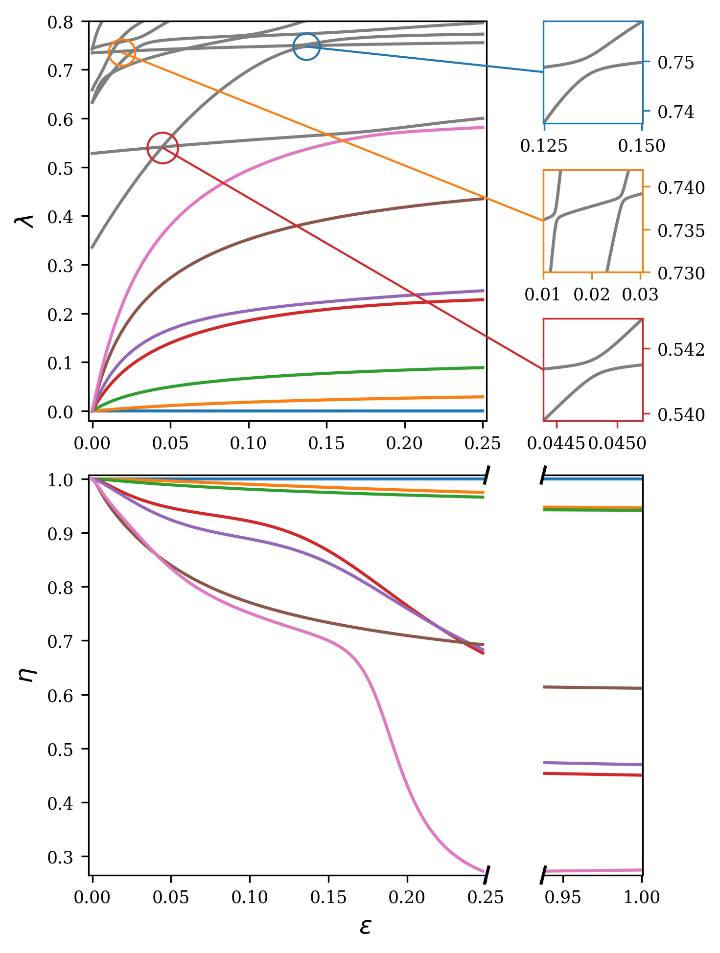
Figure 1: Top panels: Evolution of the eigenvalues of the Laplacian of (5) and (14) with $r=7$ area partitioning of the PanTaGruEl model of the synchronous grid of continental Europe. Zero-modes giving rise to inter-area oscillations are shown in color and some of the lowest non-degenerate modes in gray. The circles mark three illustrative avoided crossings. The three right panels make it clear that levels avoid crossing each other, because of the lack of specific symmetry in the system. Bottom panel: evolution of the scalar product $\eta=\mathbf{u}_{\alpha}^{\top}(\epsilon=0)\cdot\mathbf{u}_{\alpha}(\epsilon)$ between hybridized zero-modes at $\epsilon=0$ and $\epsilon$. The avoided crossing at around $\epsilon=0.2$ between the seventh (pink) mode and the first non-degenerate (grey) leads to an abrupt drop in $\eta$ for the pink mode. Almost simultaneously, there is an avoided crossing between the fourth (red) and fifth (purple) eigenvalue giving a noticeable drop in $\eta$ for both modes. The first three modes barely change their structure all the way up to $\epsilon=1$.

The hybridization of the zero-modes can be quantified via the scalar product

$$\eta=\mathbf{u}_{\alpha}^{\top}(\epsilon=0)\cdot\mathbf{u}_{\alpha}(\epsilon)\,,$$ (29)

between an unperturbed mode at $\epsilon=0$ and its vector at $\epsilon\neq 0$. The bottom panel of Fig. 1 shows that the low-lying zero-mode essentially keep their unperturbed structure, with $\eta\gtrsim 0.95$ all the way to the fully connected network limit $\epsilon\rightarrow 1$. Accordingly, the degenerate matrix perturbation theory presented above predicts the structure of the corresponding eigenvectors very well. These modes correspond to east-west inter-area oscillations [28].

We have observed, and will discuss in a follow-up paper that increasing the number $r$ of areas improves the precision with which the lowest eigenvalues and -vectors are predicted. Simultaneously, this increases the number of fast growing, initially degenerate eigenvalues, which accordingly meet the non-degenerate eigenvalues at lower values of $\epsilon$. Because they cannot cross them, however, they undergo avoided crossings which pushes back the initially non-degenerate part of the spectrum. Qualitatively, this leads to a better protection of the low-lying eigenvalues which hybridize very little. This is further illustrated in Fig. 2 which shows that the Fiedler, $\alpha=2$ mode keeps the same structure from the weakly coupled limit at $\epsilon=0.1$ to the fully coupled limit at $\epsilon=1$.

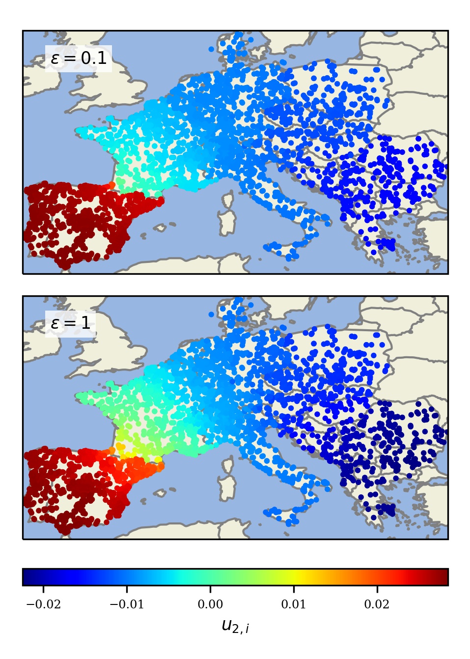
Figure 2: Structure of the Fiedler mode of the Laplacian of the PanTaGruEl model of the synchronous grid of continental Europe in the weakly (top panel) and fully (bottom) connected cases. The color corresponds to the value of the eigenvector $u_{2,i}$ of the corresponding node $i$. The mode structure is essentially the same for $\epsilon=0.1$ as for $\epsilon=1$. This mode corresponds to east-west inter-area oscillations.

To show that these modes are indeed coupled to inter-area oscillations in the grid we finally investigate abrupt 900 MW power generation faults in Portugal and in Greece. The results are shown in Fig. 3. It is seen that following such a fault, the opposite area oscillates coherently, with all nodes oscillating at the same phase and frequency, before synchronizing at a smaller frequency value.

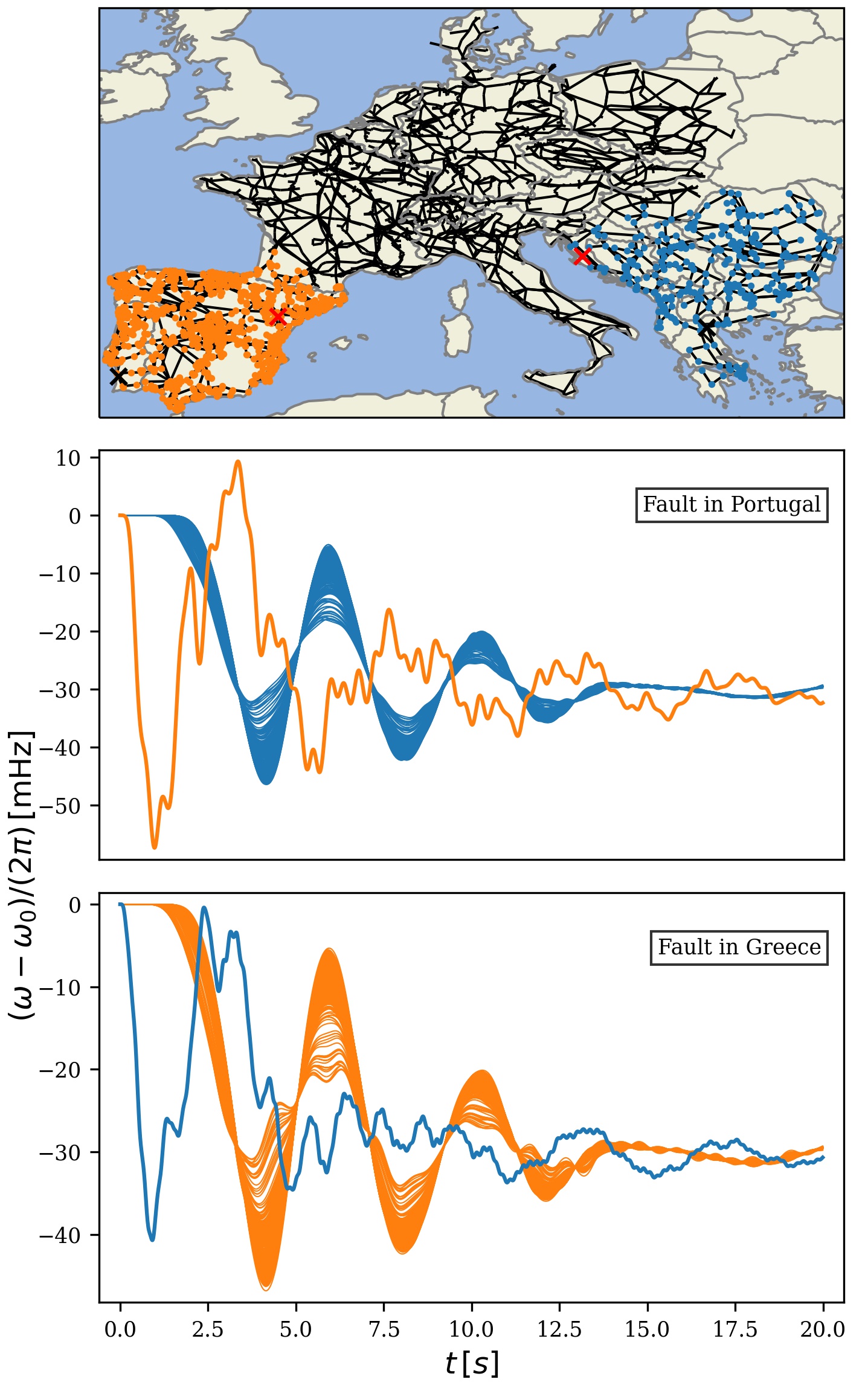
Figure 3: Time-evolution of frequencies following a 900 MW fault in Portugal (middle panel) or Greece (lower panel). The fault locations are marked by the two black crosses in the top panel. The response of all nodes in the area opposite to the fault, as well as on one node in the faulted area (red crosses in the top panel) are shown in the middle and lower panels.

VII Conclusions

We have constructed a matrix perturbation theory of slow coherent, inter-area oscillations. We have shown that inter-area oscillations emerge from the weak hybridization of some of the zero modes of coherent areas. The hybridization means that areas, even located far away from each other, are connected through a mode that is largely constant on each area. When such modes are excited, the corresponding areas oscillate coherently against each other. We finally stress that the singular perturbation theory of [12, 22] is absolutely not justified here, because the required small parameters have values $d=140$ and $\delta=37$, much larger than one. Work in progress investigates damping of inter-area oscillations and location of fault that might trigger them.

References

- [1] J. Machowski, J. W. Bialek, and J. R. Bumby, Power system dynamics: stability and control, 2nd ed. Chichester, U.K: Wiley, 2008.
- [2] G. Rogers, Power system oscillations. Springer Science & Business Media, 2012.
- [3] M. Klein, G. J. Rogers, and P. Kundur, “A fundamental study of inter-area oscillations in power systems,” IEEE Transactions on power systems, vol. 6, no. 3, pp. 914–921, 1991.
- [4] Entsoe, “Analysis of ce inter-area oscillations of 1st december 2016,” available on-line., 2017.
- [5] WECC, “Modes of inter-area power oscillations in western interconnection,” available on-line., 2013.
- [6] EPRI Final Report TR-108256, “System disturbance stability studies for western system coordinating council (wscc),” prepared by Powertech Labs Inc., 1997.
- [7] D. N. Kosterev, C. W. Taylor, and W. A. Mittelstadt, “Model validation for the august 10, 1996 wscc system outage,” IEEE Transactions on Power Systems, vol. 14, no. 3, pp. 967–979, 1999.
- [8] N. Janssens and A. Kamagate, “Interarea oscillations in power systems,” IFAC Proceedings Volumes, vol. 33, no. 5, pp. 217–226, 2000, iFAC Symposium on Power Plants and Power Systems Control 2000, Brussels, Belgium, 26-29 April 2000.
- [9] E. Grebe, J. Kabouris, S. López Barba, W. Sattinger, and W. Winter, “Low frequency oscillations in the interconnected system of continental europe,” in IEEE PES General Meeting, 2010, pp. 1–7.
- [10] X. Cheng and J. Scherpen, “Model reduction methods for complex network systems,” Annual Review of Control, Robotics, and Autonomous Systems, vol. 4, no. 1, p. null, 2021. [Online]. Available: https://doi.org/10.1146/annurev-control-061820-083817
- [11] P. V. Kokotovic, R. E. O’Malley Jr, and P. Sannuti, “Singular perturbations and order reduction in control theory—an overview,” Automatica, vol. 12, no. 2, pp. 123–132, 1976.
- [12] J. H. Chow, Ed., Time-Scale Modeling of Dynamic Networks with Applications to Power Systems. Berlin Heidelberg, Germany: Springer-Verlag, 1982.
- [13] J. H. Chow, J. Cullum, and R. A. Willoughby, “A Sparsity-Based Technique for Identifying Slow-Coherent Areas in Large Power Systems,” IEEE Transactions on Power Apparatus and Systems, vol. 103, pp. 463–473, 1984.
- [14] J. H. Chow and P. Kokotović, “Time scale modeling of sparse dynamic networks,” IEEE Transactions on Automatic Control, vol. 30, pp. 714–722, 1985.
- [15] R. Date and J. Chow, “Aggregation properties of linearized two-time-scale power networks,” IEEE Transactions on Circuits and Systems, vol. 38, pp. 720–730, 1991.
- [16] A. R. Bergen and D. J. Hill, “A Structure Preserving Model for Power System Stability Analysis,” IEEE Transactions on Power Apparatus and Systems, vol. PAS-100, no. 1, pp. 25–35, jan 1981.
- [17] Y. Yang, J. Zhao, H. Liu, Q. Z., D. J., and Q. J., “A matrix-perturbation-theory-based optimal strategy for small-signal stability analysis of large-scale power grid,” Prot. Control Mod. Power Syst., vol. 3, p. 34, 2018.
- [18] L. Pagnier and P. Jacquod, “Optimal Placement of Inertia and Primary Control: A Matrix Perturbation Theory Approach,” IEEE Access, vol. 7, pp. 145 889–145 900, 2019.
- [19] T. Coletta and P. Jacquod, “Performance Measures in Electric Power Networks Under Line Contingencies,” IEEE Transactions on Control of Network Systems, vol. 7, no. 1, pp. 221–231, mar 2020.
- [20] B. Bamieh. (2020, Feb.) A Tutorial on Matrix Perturbation Theory (using compact matrix notation). Online. [Online]. Available: arxiv:2002.05001
- [21] J. J. Sakurai and J. Napolitano, Modern Quantum Mechanics, 2nd ed. Cambridge, U.K.: Cambridge University Press, 2017.
- [22] J. H. Chow, Ed., Power System Coherency and Model Reduction. New York, NY, USA: Springer, 2013.
- [23] J. von Neumann and E. P. Wigner, “Über das Verhalten von Eigenwerten bei adiabatischen Prozessen,” Phys. Z., vol. 30, pp. 467–470, 1929.
- [24] M. Fiedler, “Laplacian of graphs and algebraic connectivity,” Banach Center Publications, vol. 25, no. 1, pp. 57–70, 1989. [Online]. Available: http://eudml.org/doc/267812
- [25] B. Mohar, “The Laplacian spectrum of graphs,” in Graph Theory, Combinatorics, and Applications. Wiley, 1991, pp. 871–898.
- [26] L. Pagnier and P. Jacquod, “Inertia location and slow network modes determine disturbance propagation in large-scale power grids,” PLOS ONE, vol. 14, no. 3, p. e0213550, mar 2019.
- [27] M. Tyloo, L. Pagnier, and P. Jacquod, “The key player problem in complex oscillator networks and electric power grids: Resistance centralities identify local vulnerabilities,” Science Advances, vol. 5, no. 11, p. eaaw8359, nov 2019.
- [28] H. Breulmann, W. Winter et al., “Analysis and Damping of Inter-Area Oscillations in the UCTE / CENTREL Power System,” CIGRÉ, Paris, France, 2000.