Symmetry-resolved entanglement for excited states and two entangling intervals in AdS₃/CFT₂

Abstract

We test the proposal of Zhao:2020qmn for the holographic computation of the charged moments and the resulting symmetry-resolved entanglement entropy in different excited states, as well as for two entangling intervals. Our holographic computations are performed in $U(1)$ Chern-Simons-Einstein-Hilbert gravity, and are confirmed by independent results in a conformal field theory at large central charge. In particular, we consider two classes of excited states, corresponding to charged and uncharged conical defects in AdS₃. In the conformal field theory, these states are generated by the insertion of charged and uncharged heavy operators. We employ the monodromy method to calculate the ensuing four-point function between the heavy operators and the twist fields. For the two-interval case, we derive our results on the AdS and the conformal field theory side, respectively, from the generating function method of Zhao:2020qmn , as well as the vertex operator algebra. In all cases considered, we find equipartition of entanglement between the different charge sectors. We also clarify an aspect of conformal field theories with a large central charge and $\hat{\mathfrak{u}}(1)_{k}$ Kac-Moody symmetry used in our calculations, namely the factorization of the Hilbert space into a gravitational Virasoro sector with large central charge, and a $\hat{\mathfrak{u}}(1)_{k}$ Kac-Moody sector.

1 Introduction

The past decade has witnessed a fruitful interplay between quantum information theory and gravity, and in particular the physics of black holes, via the AdS/CFT correspondence Maldacena . The AdS/CFT correspondence is a duality between strongly coupled gauge theories in $d$ space-time dimensions (the CFT side) and weakly coupled gravitational theories in $d+1$ dimensional Anti de Sitter space-times (the AdS side of the correspondence). A bridge between quantum information theory and gravity is laid by the Ryu-Takayanagi prescription for the holographic computation of entanglement entropy in terms of the length of a minimal geodesic in the gravitational theory RT . This triggered an avalanche of advances further translating quantum information theoretic concepts into geometric objects on the gravity side of the correspondence, for a review, c.f. RangamaniTakayanagiBook . Important examples include relative entropy MyersCasiniBlanco ; wong2013entanglement , quantum computational complexity Susskind:2014rva ; Brown:2015bva ; Brown:2015lvg , tensor networks Swingle:2009bg ; Happy , and quantum error correction HarlowAlmheiriDong ; PreskillPastawski , entwinement Erdmenger:2019lzr , entanglement entropy at genus one Gerbershagen:2021yma and entanglement measures probing the entanglement shadow Gerbershagen:2021gvc . All these examples treat CFTs at large central charge.

Most examples of quantum systems carry global symmetries. Therefore it is interesting to investigate the entanglement associated with charged sectors in the space of states. In GoldsteinSela this question was addressed by introducing the notion of symmetry-resolved entanglement entropy. It organizes the Hilbert space of a sub-interval $\mathcal{A}$ into sectors of fixed charge and quantifies the entanglement for one such sectors between $\mathcal{A}$ and its complement $\bar{\mathcal{A}}$. Since then, this line of research has been expanded in a variety of examples including free quantum field theories Bonsignori:2019naz ; Murciano:2020vgh ; tan2020particle , via dimensional reduction Murciano:2020lqq , excited states Capizzi:2020jed , symmetry-resolved relative entropy Chen:2021pls , the conformal bootstrap Horvath:2021fks ; Capizzi:2021kys , entanglement negativity Murciano:2021djk , sine-Gordon theory Horvath:2021rjd , quenches in free fermion chains Parez:2021pgq and Wess-Zumino-Witten models Calabrese:2021qdv .

In this work we discuss the holographic realization of symmetry-resolved entanglement presented in Zhao:2020qmn in charged and uncharged excited states, as well as for the case of two entangling intervals. Two main results were obtained in Zhao:2020qmn : The first was to establish a new method based on a generating function approach to determine the symmetry-resolved entanglement entropy directly from the expectation value of the sub-region charge operator $Q_{\mathcal{A}}$. This proved to be particularly efficient in the holographic calculation of symmetry-resolved entanglement entropy.

The second result of Zhao:2020qmn was the proposal of a geometric dual for symmetry-resolved entanglement entropy on the gravity side of the AdS/CFT correspondence. In Zhao:2020qmn , we studied Einstein-Hilbert gravity in $\text{AdS}_{3}$ coupled to $U(1)$ Chern-Simons gauge theory, or $U(1)$ Chern-Simons-Einstein-Hilbert gravity in short. Investigating the ground state of this theory, we identified bulk Wilson lines as the natural candidates to resolve the entanglement entropy on charge sectors. The bulk Wilson line needs to align with the Ryu-Takayanagi geodesic, as required to sustain the replica symmetry of the Rényi entropy. Using our generating function method, we holographically derived the charged moments and the symmetry-resolved entanglement entropy for a CFT with $\hat{\mathfrak{u}}(1)_{k}$ Kac-Moody symmetry. The concrete examples studied were the case of a single entangling interval in the ground state both on the gravity and CFT side, as well as conical defect solutions on the gravity side. Since our holographic theory carries a large central charge, we checked our holographic result against a CFT calculation at large central charge with $U(1)$ symmetry. The key observation in Zhao:2020qmn was that the bulk Wilson line is dual to a charge defect in the CFT, which is naturally described by a pair of $U(1)$ vertex operators inserted at the endpoints of the entangling region.

While our previous work Zhao:2020qmn focused mostly on the ground state, it is the aim of this work to test our Wilson line proposal in various excited states of the gravitational theory, and confirm each result with the corresponding CFT calculation at large central charge. As argued in Zhao:2020qmn , the leading order contribution in entanglement is entirely fixed by replica symmetry and conformal symmetry. The examples studied in the present paper corroborate the efficiency of our generating function approach, circumventing the potentially laborious computation of the charged moments. Moreover, we compute the symmetry-resolved entanglement entropy for the case of two disconnected entanglement intervals in the ground state. While examples of the symmetry-resolved entanglement entropy for excited states can already be found in the literature for systems with small central charge, see for instance Capizzi:2020jed , the case of holographic CFTs has only recently drawn attention Zhao:2020qmn . The case of two entangling intervals is, to the best of our knowledge, completely unexplored so far.

Our paper is structured as follows: Section 2 is devoted to the AdS₃ side of the duality: In Section 2.1, we first review the symmetry-resolved entanglement entropy along the lines of GoldsteinSela , as well as the generating functional method of Zhao:2020qmn . We focus on the main points of the calculation of the holographic charged moments in section 2.2. In section 2.3 we summarize the results of Zhao:2020qmn for the symmetry-resolved entanglement entropy in the single interval case, and present a new result for an AdS₃ background with a nonvanishing charge generated by the insertion of a pair of charged vertex operators. In section 2.4, we present the AdS₃ calculation for the case of two disjoint intervals. In section 3, we present our CFT results. In section 3.1, we present arguments for the factorization of the Hilbert space of $U(1)$ Chern-Simons-Einstein-Hilbert gravity in a gravitational and a Kac-Moody sector, as well as the corresponding statement on the CFT side. In section 3.2, we use this factorization property to rederive the charged moments and symmetry-resolved entanglement entropy for an uncharged excited state. In section 3.3, we derive corresponding results for the CFT vacuum with a background charge. In section 3.4, we finally calculate the symmetry-resolved entanglement entropy for two disjoint intervals. We conclude and give an outlook in section 4. Details on an alternative derivation for the case of two intervals and of the $n=2$ Rényi entropy using the Knizhnik-Zamolodchikov equation and the $U(1)$ Ward identity are presented in appendix A.

2 Symmetry resolved entanglement in AdS₃

Given any theory with global symmetry $G$, its Hilbert space of states decomposes into irreducible representations, each corresponding to a sector of fixed charge. Then it is possible to investigate the entanglement associated with single charge sectors, i.e. the symmetry-resolved entanglement entropy. In this section, we the review previous results on the symmetry-resolved entanglement entropy of Zhao:2020qmn and extend them to more general cases.

2.1 Symmetry resolved entanglement and the generating function method

We consider a system with an internal $U(1)$ symmetry and a bipartition of its Hilbert space $\mathcal{H}=\mathcal{H}_{\mathcal{A}}\otimes\mathcal{H}_{\mathcal{B}}$, associated with constant time spatial region $\mathcal{A}$ and its complement $\mathcal{B}$. We assume that the charge operator generating the $U(1)$ symmetry splits diagonally, $Q=Q_{\mathcal{A}}\oplus Q_{\mathcal{B}}$. Moreover, we restrict to eigenstates of $Q$ with density matrix $\rho$ , i.e. $[\rho,Q]=0$, implying that, after tracing out $\mathcal{B}$, we have $[\rho_{\mathcal{A}},Q_{\mathcal{A}}]=0$. Therefore $\rho_{\mathcal{A}}$ is block-diagonal, with each block corresponding to an eigenvalue $q$ of the sub-region charge operator $Q_{\mathcal{A}}$,

$$\rho_{\mathcal{A}}=\oplus_{q}\rho_{\mathcal{A}}(q)\ ,$$ (2.1)

A block $\rho_{\mathcal{A}}(q)$ is singled out by the projector $\Pi_{q}$ onto the eigenspace of $Q_{\mathcal{A}}$ with fixed eigenvalue $q$,

$$\rho_{\mathcal{A}}(q)=\rho_{\mathcal{A}}\Pi_{q}\ .$$ (2.2)

Each eigenvalue $q$ is measured with probability

$$P_{\mathcal{A}}(q)=\frac{\mathrm{Tr}\rho_{\mathcal{A}}(q)}{\mathrm{Tr}\rho_{\mathcal{A}}}=\mathrm{Tr}\rho_{\mathcal{A}}(q)\,$$ (2.3)

to appear in a measurement of $Q_{\mathcal{A}}$, since $\rho_{\mathcal{A}}$ is normalized, $\mathrm{Tr}\rho_{\mathcal{A}}=1$. The block-diagonal structure of $\rho_{\mathcal{A}}$ enforces a block decomposition of $\rho_{\mathcal{A}}^{n}$,

$$\rho_{\mathcal{A}}^{n}=\oplus_{q}\rho_{\mathcal{A}}(q)^{n}\quad\text{with}\quad\rho_{\mathcal{A}}(q)^{n}=\left(\rho_{\mathcal{A}}\Pi_{q}\right)^{n}=\rho_{\mathcal{A}}^{n}\Pi_{q}\,,$$ (2.4)

and the probability distribution of a charge block in $\rho_{\mathcal{A}}^{n}$ is given by

$$P_{\mathcal{A},n}(q)=\frac{\mathrm{Tr}\rho_{\mathcal{A}}(q)^{n}}{\mathrm{Tr}\rho_{\mathcal{A}}^{n}}\,.$$ (2.5)

The decompositions (2.1) and (2.4) can be used to define the symmetry-resolved Rényi entropy,

$$S_{n}(q)=\frac{1}{1-n}\log\mathrm{Tr}\left(\frac{\rho_{\mathcal{A}}(q)}{P_{\mathcal{A}}(q)}\right)^{n}=\frac{1}{1-n}\log{\frac{\mathcal{Z}_{n}(q)}{\mathcal{Z}_{1}(q)^{n}}}\ ,$$ (2.6)

where we denote

$$\mathcal{Z}_{n}(q)=\mathrm{Tr}\rho_{\mathcal{A}}(q)^{n}=\mathrm{Tr}\left[\rho_{\mathcal{A}}^{n}\Pi_{q}\right]\ ,$$ (2.7)

The entropies (2.6) are measures of the amount of entanglement between the subsystems $\mathcal{A}$ and $\mathcal{B}$ in each charged block.

The symmetry-resolved entanglement entropy in the $q$-sector is given by the $n\to 1$ limit of $S_{n}(q)$,

$$S_{1}(q)=\lim_{n\to 1}S_{n}(q)=-\mathrm{Tr}\left[\frac{\rho_{\mathcal{A}}(q)}{P_{\mathcal{A}}(q)}\log\left(\frac{\rho_{\mathcal{A}}(q)}{P_{\mathcal{A}}(q)}\right)\right]\ .$$ (2.8)

From (2.1) and (2.8), the total entanglement entropy associated with $\rho_{\mathcal{A}}$ decomposes into

$$S_{1}=\sum_{q}P_{\mathcal{A}}(q)S_{1}(q)-\sum_{q}P_{\mathcal{A}}(q)\log P_{\mathcal{A}}(q)\ .$$ (2.9)

The two terms in (2.9) are usually referred to as configurational and fluctuation entropy, respectively Lukin256 , the former being related to the operationally accessible entanglement entropy WisemanVaccaro ; BarghathiHerdman ; BarghathiCasiano .

As can be seen from (2.6), calculating $\mathcal{Z}_{n}(q)$ is necessary to obtain the symmetry-resolved Rényi and entanglement entropies. However, this is generally very involved as it demands knowledge of the spectrum of the reduced density matrix $\rho_{\mathcal{A}}$ and its resolution in $Q_{\mathcal{A}}$. Therefore, the idea advocated in GoldsteinSela is rather to compute the charged moments

$$\mathcal{Z}_{n}(\mu)=\mathrm{Tr}\left[\rho_{\mathcal{A}}^{n}e^{i\mu Q_{\mathcal{A}}}\right]\,.$$ (2.10)

These are related to (2.7) by Fourier transformation,

$$\mathcal{Z}_{n}(q)=\int_{-\infty}^{\infty}\frac{d\mu}{2\pi}e^{-i\mu q}\mathcal{Z}_{n}(\mu)\,,$$ (2.11)

for the case of $q\in\mathbbm{R}$. For discrete eigenvalues, for example if $\mathcal{Z}_{n}(\mu)=\mathcal{Z}_{n}(\mu+2\pi)$, the range of integration (2.11) changes to $[-\pi,\pi]$.

While the charged moments (2.10) provide a way to calculate the symmetry-resolved entropies, they are not easily computed for general excited states (c.f. Capizzi:2020jed ; Horvath:2020vzs ; Bonsignori:2020laa ). Based on a generating function, a new method which simplifies the calculation was introduced in Zhao:2020qmn . It extracts the charged moments and hence the symmetry-resolved entanglement entropy directly from the expectation value of the sub-region charge operator $Q_{\mathcal{A}}$, which is generally easier to compute than the charged moments themselves. Here we recapitulate this method and in subsequent sections we provide examples corroborating its efficiency in the context of holography.

Define a normalized generating function associated with the charged moments $\mathcal{Z}_{n}(\mu)$ as

$$f_{n}(\mu)\coloneqq\frac{\mathcal{Z}_{n}(\mu)}{\mathcal{Z}_{n}(0)}=\frac{\mathcal{Z}_{n}(\mu)}{\mathcal{Z}_{n}},$$ (2.12)

fulfilling the initial condition

$$f_{n}(0)=1\,.$$ (2.13)

The expectation value of $Q_{A}$ is then expressed as

$$\langle iQ_{\mathcal{A}}\rangle_{n,\mu}:=\frac{\mathrm{Tr}\left[iQ_{\mathcal{A}}\rho^{n}e^{i\mu Q_{\mathcal{A}}}\right]}{\mathrm{Tr}\left[\rho^{n}e^{i\mu Q_{\mathcal{A}}}\right]}=\frac{\partial\ln\mathcal{Z}_{n}(\mu)}{\partial\mu}=\frac{\partial\ln f_{n}(\mu)}{\partial\mu}\ .$$ (2.14)

In order to evaluate $f_{n}(\mu)$, and hence $Z_{n}(\mu)$, it suffices to know the expectation value of the charge, and integrate (2.14) with initial condition (2.13).

As evident from (2.5), (2.7) and (2.11), the probability distribution $P_{\mathcal{A},n}(q)$ can be recast in terms of the generating function by a Fourier transformation,

$$P_{\mathcal{A},n}(q)=\frac{\mathcal{Z}_{n}(q)}{\mathcal{Z}_{n}}=\int_{-\infty}^{\infty}\frac{d\mu}{2\pi}e^{-i\mu q}f_{n}(\mu)\ ,$$ (2.15)

As pointed out in Capizzi:2020jed , the symmetry-resolved Rényi entropy,

$$S_{n}(q)=S_{n}+\frac{1}{1-n}\log{\frac{P_{\mathcal{A},n}(q)}{P_{\mathcal{A}}(q)^{n}}}\ ,$$ (2.16)

as well as the symmetry-resolved entanglement entropy

$$S(q)=S+\lim_{n\to 1}\frac{1}{1-n}\log{\frac{P_{\mathcal{A},n}(q)}{P_{\mathcal{A}}(q)^{n}}}\ ,$$ (2.17)

split into two pieces. The first are their uncharged counterparts, the Rényi entropy $S_{n}$ and the entanglement entropy $S$, while the charge information resides fully in the second contribution.

2.2 Holographic charged moments

The holographic dual of charged moments in $U(1)$ Chern-Simons-Einstein gravity was first discussed in Belin:2013uta . Here we follow the Wilson line defect prescription of Zhao:2020qmn , and briefly review the holographic interpretation of the charged moments.

In $U(1)$ Chern-Simons-Einstein-Hilbert gravity, two additional chiral gauge fields are introduced on top of the gravitational sector. The asymptotic behavior of the left-moving gauge field takes the following form in Fefferman-Graham coordinates Kraus:2006wn ,

$$A=A^{(0)}+e^{-2\rho}A^{(2)}+\cdots\ \quad\textrm{as}\quad\rho\to\infty\ ,$$ (2.18)

where $\rho$ is the radial coordinate in AdS and, for convenience, we have set the AdS radius $l=1$. Under this asymptotic expansion and employing the boundary condition $A^{(0)}_{\rho}=0$, the variation of the action with respect to $A$ yields Kraus:2006wn

$$\delta I_{A}=\frac{i}{2\pi}\int_{\partial\mathcal{M}}d^{2}x\sqrt{g^{(0)}}J^{a}\delta A_{a}^{(0)}\,.$$ (2.19)

Here, $J^{a}$ is identified as the boundary $U(1)$ current whose components in complex coordinates read

$$J_{w}=\frac{1}{2}J^{\bar{w}}=\frac{ik}{2}A_{w}^{(0)}\ ,\quad J_{\bar{w}}=0\ ,$$ (2.20)

Since $J_{\bar{w}}$ always vanishes, the corresponding source term is $A^{(0)}_{\bar{w}}$. By the AdS/CFT correspondence, in the presence of a source term, the CFT action is deformed as Kraus:2006nb ; Kraus:2006wn

$$I_{CFT}\to I_{CFT}+\frac{i}{2\pi}\int_{\partial\mathcal{M}}d^{2}wJ^{\bar{w}}A^{(0)}_{\bar{w}}\ .$$ (2.21)

The left-moving sub-region charge on $\mathcal{A}$ is defined as

$$q_{\mathcal{A}}=\int_{\mathcal{A}}\frac{dw}{2\pi i}J_{w}\ .$$ (2.22)

The idea relating the charged moments with the deformation of the CFT action sets out by rewriting the sub-region charge (2.22) as a two-dimensional integral over the boundary Riemann surface $\partial\mathcal{M}$. For instance, considering $\mathcal{A}$ to be a single interval and denoting the endpoints of the interval $\mathcal{A}$ as $w=z_{1}$ and $w=z_{2}$, one can rewrite (2.22) as

$$q_{\mathcal{A}}=\int_{z_{2}}^{z_{1}}\frac{dw}{2\pi i}J_{w}=\int_{\partial\mathcal{M}}\frac{d^{2}w}{2\pi i}\left(G(\bar{w},\bar{z}_{1})-G(\bar{w},\bar{z}_{2})\right)J_{w}\ ,$$ (2.23)

where $G(\bar{w},\bar{z})$ is the Green kernel of the $\partial$ operator defined on the boundary Riemann surface. Therefore, the additional operator in the charged moments can be thought of as introducing an additional source term coupled to the $U(1)$ current, where the additional source reads

$$\delta A^{(0)}_{\bar{w}}=i\mu\left(G(\bar{w},\bar{z}_{1})-G(\bar{w},\bar{z}_{2})\right)\ .$$ (2.24)

As shown in Zhao:2020qmn , this kind of source is realized in the bulk by introducing a $U(1)$ Wilson line defect action

$$I_{d}=-\frac{ik\mu}{2\pi}\int_{\mathcal{C}}A\,,$$ (2.25)

where the curve $\mathcal{C}$ is anchored at the endpoints of the boundary interval $\mathcal{A}$ and is required to be orthogonal to the boundary when approaching spatial infinity. Observe that the $U(1)$ defect action is actually topological in the bulk.

In principal, different choices of the curve $\mathcal{C}$ result in different gauge field configurations in the bulk. As argued in Zhao:2020qmn a natural choice of the curve $\mathcal{C}$ is the geodesic anchored at the endpoints of $\mathcal{A}$. It was shown in Zhao:2020qmn that approaching spatial infinity, independent of the shape of the Wilson line, the field strength always takes the form

$$\lim_{\rho\to\infty}F =F_{w\bar{w}}dw\wedge d\bar{w}$$

$$=2\mu\left(\delta^{(2)}(w-z_{1},\bar{w}-\bar{z}_{1})-\delta^{(2)}(w-z_{2},\bar{w}-\bar{z}_{2})\right)dw\wedge d\bar{w}\,.$$ (2.26)

Hence, the leading order in the asymptotic expansion of the gauge field $A$ is fixed as

$$A^{(0)}_{w} =a(w)-i\mu\left(G(w,z_{1})-G(w,z_{2})\right)\,,$$

$$A^{(0)}_{\bar{w}} =\bar{a}(\bar{w})+i\mu\left(G(\bar{w},\bar{z}_{1})-G(\bar{w},\bar{z}_{2})\right)\,.$$ (2.27)

Here, $a(w)$ and $\bar{a}(\bar{w})$ denote general background connections. From this the current (2.20) is read out and the sub-region charge as well as the generating function $f_{n}(\mu)$ can be computed.

2.3 Symmetry resolved entanglement for a single interval

In this section we holographically derive the symmetry-resolved entanglement entropy for excited states and a single entangling interval. The contribution from the Wilson line defect to the charged moments and the generating function $f_{n}(\mu)$ is determined by the complex structure of the boundary replica $n$-fold, without being affected by the details of the bulk geometry. Furthermore, we show that the probability distributions $P_{\mathcal{A},n}(q)$ are the Gaussian distributions of the charge fluctuations in the general case. This demonstrates that the symmetry-resolved entanglement entropy is independent of the sub-region charge in all these cases for holographic $U(1)$ Chern-Simons theory.

For Poincaré $AdS_{3}$, we denote the boundary complex coordinates as $z$ and $\bar{z}$. Without loss of generality, we consider a background gauge field $A$ with general asymptotic expansion

$$A_{z}=a(z)+\cdots\ ,\quad\quad A_{\bar{z}}=\bar{a}(\bar{z})+\cdots\quad\textrm{as}\quad\rho\to\infty$$ (2.28)

where the leading order terms in (2.28) imply a non-vanishing background $U(1)$ current. For a single boundary interval with endpoints located at $z=z_{1}$ and $z=z_{2}$, the charged moments $\mathcal{Z}_{n}(\mu)$ are constructed by inserting the Wilson line defect (2.25) in the bulk repica $n$-fold. Since we are interested in the sub-region charge giving rise to the charged moments $\mathcal{Z}_{n}(\mu)$, in order to employ (2.2), we need the Green kernel of $\partial_{\bar{z}}$ on the replica $n$-fold. This can be derived from the Green kernel in the complex plane,

$$G(\bar{z},\bar{z}_{i})=\frac{1}{2\pi}\frac{1}{\bar{z}-\bar{z}_{i}}\ ,\quad i=1,2\ ,$$ (2.29)

as follows. The topology of the replica $n$-fold is still a Riemann sphere in the single interval case. The replica $n$-fold is mapped to a single complex $\xi$-plane by the uniformization mapping

$$\xi=\left(\frac{z-z_{2}}{z-z_{1}}\right)^{\frac{1}{n}}\,.$$ (2.30)

A fixed $z$ corresponds to $n$ different values of $\xi$. The mapping (2.30) can be used to obtain the Green kernel of the replica $n$-fold in $z$-coordinates as

$$G^{(n)}(\bar{z},\bar{z}_{i})=\left(\frac{d\xi}{dz}\right)G(\bar{\xi},\bar{\xi}_{i})=\frac{1}{2\pi n}\frac{1}{\bar{z}-\bar{z}_{i}}\ ,\quad i=1,2\ .$$ (2.31)

It is this Green kernel which, when plugged into (2.2), provides the gauge field configuration for the $\mathcal{Z}_{n}(\mu)$ charged moments.

The next task is to obtain the background gauge field in the replica $n$-fold without additional $U(1)$ Wilson line defect insertion. As we show below, the leading order of the Chern-Simons connection in the replica $n$-fold always takes the same form as the background solution in (2.28). The differences between them are hidden in the $n$-sheeted coordinates $z$ and $\bar{z}$. In fact, the connection in the replica $n$-fold is an analytic continuation of the background connection from the original manifold.

Indeed, consider a background gauge field $a(z)$ in (2.28) generated by the boundary operator excitations located at $z=0$ and $z=\infty$.

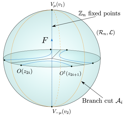
Figure 1: For a single entangling interval, the universal covering of the replica $n$-fold is a Riemann sphere. There are $n$ copies of excitations on the replica $n$-fold. The blue lines represent the bulk Wilson lines dual to the boundary excitations. The orange lines represent the branch cuts between the $n$ sheets in the original replica manifold.

Due to this pole structure, the connection can be written as $a(z)=\frac{\alpha}{z}$, with $\alpha$ some constant associated with the charge of the excited operators. As shown in figure 1, in the replica trick, one inserts $n$ copies of the excited operators in the replica $n$-fold, which are located on each sheet at $z_{2m-1}=0$ and $z_{2m}=\infty$ $(m=1,\cdots,n)$, with $m$ denoting the $m^{\text{th}}$ sheet of the replica $n$-fold. By the uniformization mapping (2.30), the excited operators are mapped to the new $2n$ points $\xi_{2m-1}=\left(\frac{z_{2}}{z_{1}}\right)^{\frac{1}{n}}e^{2\pi im/n}$ and $\xi_{2m}=e^{2\pi im/n}$ $(m=1,\cdots,n)$. Therefore, in the complex $\xi$-plane, one can write the leading order background connection in the replica $n$-fold as

$$A^{(0)}_{\xi}=\sum_{m=1}^{n}\left(\frac{\alpha}{\xi-\xi_{2m-1}}-\frac{\alpha}{\xi-\xi_{2m}}\right)\,.$$ (2.32)

The connection (2.32) on the replica $n$-fold is related to the original connection $a(z)=\frac{\alpha}{z}$ by a conformal transformation, hence

$$A^{(0)}_{\xi}\left(\frac{d\xi}{dz}\right)=a(z)\,.$$ (2.33)

In the $n$-sheeted $z$-coordinates, the background connection of the replica $n$-fold hence still takes the same form as the original connection $a(z)$.

We are now ready to derive the sub-region charge with an additional Wilson line defect insertion. From (2.22) together with (2.20) it follows that

$$q_{\mathcal{A}} =\frac{ik}{2}\int_{z_{2}+\delta}^{z_{1}-\delta}\frac{dz}{2\pi i}\left(a(z)-i\mu G^{(n)}(z,z_{1})+i\mu G^{(n)}(z,z_{2})\right)$$

$$=q_{0}+\frac{ik\mu}{4\pi}\log{\left(\frac{z_{1}-z_{2}}{\delta}\right)}\,.$$ (2.34)

Here $q_{0}=\frac{ik}{2}\int_{z_{2}}^{z_{1}}\frac{dz}{2\pi i}\ a(z)$ is the left-moving background sub-region charge, which is finite. The right-moving part takes an analogous form. The definition of the generating function (2.14) then implies

$$f_{n}(\mu) =\exp{\left(i\int_{0}^{\mu}d\mu^{\prime}\ \langle\hat{Q}_{\mathcal{A}}\rangle_{n,\mu^{\prime}}\right)}=e^{i\mu Q_{0}}\cdot\left|\frac{v_{1}-v_{2}}{\delta}\right|^{-\frac{k}{n}(\frac{\mu}{2\pi})^{2}}\,,$$ (2.35)

where $Q_{0}=q_{0}+\bar{q}_{0}$ is the total sub-region charge originating purely from the background solutions (2.28). Using the regularized length of the geodesic in Poincaré AdS,

$$L=2\ln{\left|\frac{v_{1}-v_{2}}{\delta}\right|}\ ,$$ (2.36)

where $\delta$ is related to the bulk UV-cutoff $\rho_{0}$ via $\delta=e^{-\rho_{0}}$, and is the cutoff around the boundary endpoints of $\mathcal{A}$. The sub-region charge and the normalized generating function are expressed through

$$\langle\hat{Q}_{\mathcal{A}}\rangle_{n,\mu}=Q_{0}+\frac{ik\mu}{4\pi^{2}n}L\ ,\quad f_{n}(\mu)=e^{i\mu Q_{0}-\frac{k}{2n}(\frac{\mu}{2\pi})^{2}L}\ .$$ (2.37)

The Fourier transformation of $f_{n}(\mu)$ in (2.37) yields the probability distribution $P_{\mathcal{A},n}(q)$

$$P_{\mathcal{A},n}(q)=\int_{-\infty}^{\infty}\frac{d\mu}{2\pi}e^{-i\mu q}f_{n}(\mu)=\sqrt{\frac{2\pi n}{kL}}e^{-\frac{2n\pi^{2}\Delta q^{2}}{kL}}\,,$$ (2.38)

where the fluctuation of the sub-region charge is denoted by $\Delta q=q-Q_{0}$. The resulting symmetry-resolved entanglement entropy (2.17) is then easily obtained,

$$S(q)=S+\lim_{n\to 1}\frac{1}{1-n}\log{\frac{P_{\mathcal{A},n}(q)}{P_{\mathcal{A}}(q)^{n}}}=\frac{c}{6}L-\frac{1}{2}\ln{\left(\frac{kL}{2\pi}\right)}+O(1)\ ,$$ (2.39)

where the entanglement entropy $S$ in three dimensions is given by the Ryu-Takayanagi formula RT $S=\frac{c}{6}L$. In (2.39), the charge dependence has disappeared in the final result, i.e. there is equipartition of entanglement amongst the charge sectors Xavier:2018kqb .

For global AdS or conical defect solutions, one obtains the symmetry-resolved entanglement entropy straightforwardly from the above procedure as well. The main difference to the case of Poincaré AdS, c.f. (2.31), is that the boundary Green kernel now takes the form

$$G^{(n)}(w,w_{i})=\frac{1}{2\pi n}\frac{e^{iw_{i}}}{e^{iw}-e^{iw_{i}}}\,,\quad w=\phi+it_{E}\,.$$ (2.40)

Here $w$ are Euclidean cylinder coordinates. As shown in Zhao:2020qmn , the final result for the symmetry-resolved entanglement entropy in the case of global AdS or conical defects is given by

$$S(q)=S-\frac{1}{2}\log{\left(\frac{kL_{1}}{2\pi}\right)}+O(1)\ ,\quad L_{1}=2\log\left|\frac{2}{\delta}\sin\frac{\Delta\phi}{2}\right|\,,$$ (2.41)

where $\Delta\phi$ is the angular extend of the boundary interval, and $S$ is the usual entanglement entropy contribution. An interesting point is that the contribution from the $U(1)$ sector in (2.41) is not sensitive to the existence of the conical defects at all. In other words, the contribution from the $U(1)$ sector is completely topological, and only senses the complex structure of the boundary Riemann surface. This is to be expected from the topological nature of the bulk Chern-Simons theory, whose only propagating degrees of freedom are boundary photons belin2020bulk . Again, the equipartition still holds in all those cases.

2.4 Symmetry resolved entanglement for two disjoint intervals

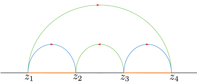
(a)

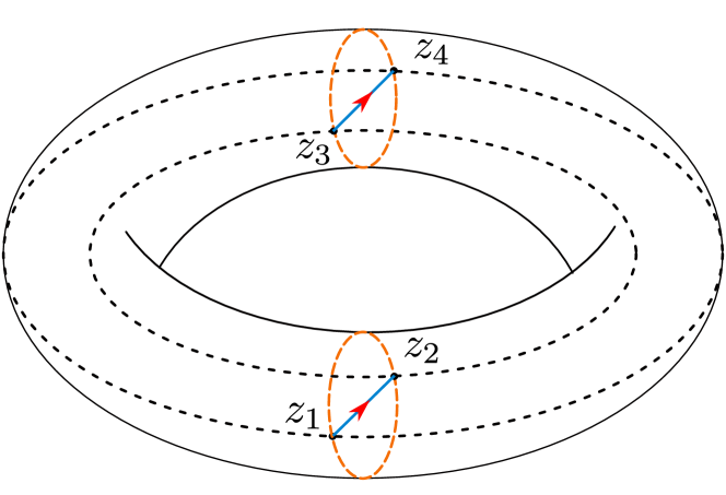
(b)

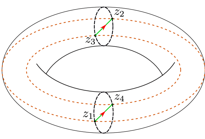
(c)

Figure 2: (a) Shows the two different configurations of the Wilson lines in the bulk replica $n$-fold, where the blue and green lines are the Wilson lines dual to the $s$-channel and $t$-channel of the four point function of charged twist operators, respectively. The red arrows indicate the direction of the field strength. (b) and (c) show the bulk constructions in the universal covering of the replica $2$-fold corresponding to $s$-channel and $t$-channel, respectively. In each phase, the Wilson lines always follow the locus of the $\mathbb{Z}_{2}$ fixed points of the torus, which are the geodesics with minimal length. The branch cuts are represented by the orange lines, which are contractible circles in the $s$-channel and non-contractible in the $t$-channel.

In this section, we consider the case of two disjoint intervals. Following Zhao:2020qmn , for an entangling region $A=A_{1}\cup A_{2}$ consisting of two disjoint intervals $A_{1}\cap A_{2}=\varnothing$ with endpoints located at $z=z_{i}$ $(i=1,2,3,4)$, the holographic dual of the CFT charged moments is given by inserting two $U(1)$ Wilson lines along the locus of the $\mathbb{Z}_{n}$ replica symmetry fixed points in the bulk. Due to the phase transition in the Rényi entropy in the two interval case, there exist two different bulk Wilson line defect configurations, as we shown in figure 2. Although the bulk constructions are different, we show that the contribution to the charged moments from the $U(1)$ sector are identical. Again, we find equipartition behavior.

We consider Poincaré AdS with vanishing background gauge field. The calculation for the sub-region charge is still straightforward. Analogous to (2.24), in the two interval case, the charged moments $\mathcal{Z}_{n}(\mu)$ require the introduction of a source term,

$$A^{(0)}_{\bar{z}}=\frac{i\mu}{2\pi n}\sum_{m=1}^{2}\left(\frac{1}{\bar{z}-\bar{z}_{2m-1}}-\frac{1}{\bar{z}-\bar{z}_{2m}}\right)\,.$$ (2.42)

The corresponding holomorphic part of the connection reads

$$A^{(0)}_{z}=-\frac{i\mu}{2\pi n}\sum_{m=1}^{2}\left(\frac{1}{z-z_{2m-1}}-\frac{1}{z-z_{2m}}\right)\,.$$ (2.43)

Evaluating the sub-region charge yields the generating function

$$f_{n}(\mu)=\left|\frac{(z_{1}-z_{2})(z_{3}-z_{4})(z_{1}-z_{4})(z_{2}-z_{3})}{\delta^{2}(z_{1}-z_{3})(z_{2}-z_{4})}\right|^{-\frac{k\mu^{2}}{4\pi^{2}n}}$$ (2.44)

The symmetry-resolved entanglement entropy is given by

$$S(q)=S-\frac{1}{2}\log\left(\frac{k}{\pi}\log\left|\frac{(z_{1}-z_{2})(z_{3}-z_{4})(z_{1}-z_{4})(z_{2}-z_{3})}{\delta^{2}(z_{1}-z_{3})(z_{2}-z_{4})}\right|\right)\,.$$ (2.45)

This rather simple calculation contains a nontrival bulk interpretation for the Wilson line defect configurations. Observe that the phase transition for symmetry-resolved entanglement entropy still takes place at the usual critical point, i.e. $x=\frac{(z_{1}-z_{2})(z_{3}-z_{4})}{(z_{1}-z_{3})(z_{2}-z_{4})}=\frac{1}{2}$. It arises from different dominating contributions in the $s$- and $t$-channel of the four point function of twist operators Hartman:2013mia . On the CFT side, these two situations are represented by imposing trivial monodromy conditions for different cycles Hartman:2013mia around points $(z_{1},z_{2})$ or $(z_{2},z_{3})$, respectively.

On the gravity side, these two different monodromy conditions indicate which circle of the bulk geometry is contractible faulkner2013 . Both bulk constructions should preserve the $\mathbb{Z}_{n}$ symmetry. What distinguishes the two phases is the locus of the bulk $\mathbb{Z}_{n}$ fixed points. Since the $U(1)$ Wilson lines are required to respect the $\mathbb{Z}_{n}$ symmetry in the two different phases, they follow different paths in the replica manifold, i.e. the respective $Z_{n}$ fixed points. Nevertheless, the boundary value of the gauge field takes the same form (2.42) in $z$-coordinates. As a result, the phase transition in the symmetry-resolved entanglement entropy is not affected by the $U(1)$ sector, and happens at the same cross ratio as for entanglement and Rényi entropies.

3 Symmetry resolved entanglement in CFT₂

In this section we confirm our holographic calculations with CFT results at large central charge. We begin in section 3.1 with an analysis of the space of states of the CFT, which was implicitly employed in Zhao:2020qmn . Namely, we argue that the total Hilbert space $\mathcal{H}_{tot}$ factorizes into a gravity sector $\mathcal{H}_{g}$ and a $\hat{\mathfrak{u}}(1)_{k}$ Kac-Moody sector $\mathcal{H}_{k}$. This paves the way to first reproduce the vacuum charged moments, after which we present CFT calculations of charged moments and symmetry-resolved entanglement entropy for the holographic dual of the conical defect solution in section 3.2, charged Poincaré AdS in section 3.3 and investigate the two interval case in section 3.4.

3.1 Factorization of the Hilbert space

We now investigate the structure of the Hilbert space of the boundary theory by taking a close look at bulk theory. Since we are working in the bottom-up set-up of the AdS/CFT correspondence, the Hilbert space for the bulk (or boundary) theory is only a subspace of the full Hilbert space in a putative full UV complete top-down approach. In particular, the decoupling of the bulk $U(1)$ Chern-Simons field from the bulk metric implies that one can change the configuration of the $U(1)$ gauge field without affecting the bulk geometry. This indicates that the bulk states considered here are factorized into a gravitational part and a $U(1)$ part. We exclude situations in which this factorization will not hold, for example in the presence of additional charged bulk fields which are coupled to both the metric and the $U(1)$ gauge field KrausPrivate , or bottom-up models with a different symmetry structure such as e.g. Einstein-Maxwell perez2016asymptotic .

Evidence for this factorization property can be traced back to the asymptotic symmetry algebra of $U(1)$ Chern-Simons-Einstein-Hilbert theory, which is the starting point of our CFT analysis. As shown in Zhao:2020qmn , the modes of the stress tensor can be expressed as $L_{n}=L_{n}^{g}+L_{n}^{k}$, where $L_{n}^{g}$ and $L_{n}^{k}$ are the Virasoro modes in the gravity and the $\hat{\mathfrak{u}}(1)_{k}$ sector, respectively. From the bulk decoupling of the metric and $\hat{\mathfrak{u}}(1)_{k}$ sector it follows that $[L_{n}^{g},L_{m}^{k}]=0$ and $[L_{n}^{g},J_{m}]=0$. This split stress-energy tensor reproduces the correct Kac-Moody algebra

$$[J_{n},J_{m}] =\frac{1}{2}nk\delta_{m+n}\ ,$$

$$[L_{n},J_{m}] =-mJ_{n+m}\ ,$$

$$[L_{n},L_{m}] =(n-m)L_{n+m}+\frac{c}{12}(n^{3}-n)\delta_{n+m,0}\ ,$$ (3.1)

where the central charge is the Brown-Henneaux central charge $c_{g}=\frac{3l}{2G_{3}}$ shifted by the central charge of the $\hat{\mathfrak{u}}_{1}(k)$ theory $c_{k}=1$, i.e. $c=c_{g}+c_{k}$. A detailed analysis for the effective central charge of the $U(1)$ Chern-Simons Einstein gravity is provided in belin2020bulk . Due to the vanishing commutators $[L_{n}^{g},L_{m}^{k}]=0$ and $[L_{n}^{g},J_{m}]=0$, (3.1) decomposes into a gravitational Virasoro algebra for $L_{n}^{g}$, and a Kac-Moody algebra for $(L_{n}^{k},J_{m})$. This decomposition of symmetry algebras leads to a decomposition of the Hilbert space into a product of sums of irreducible representations of the gravitational Virasoro and the Kac-Moody algebra, respectively,

$$\mathcal{H}_{tot}=\mathcal{H}_{g}\otimes\mathcal{H}_{k}\,.$$ (3.2)

The density matrix of the system inherits this structure from Hilbert space

$$\rho=\rho_{g}\otimes\rho_{k}\,.$$ (3.3)

This leads to a decoupling of the the charged moments in the two sectors, (2.10),

$$\mathcal{Z}_{n}(\mu) =\mathrm{Tr}\left[(\rho_{\mathcal{A},g}^{n}\otimes\rho_{\mathcal{A},k}^{n})e^{i\mu Q_{\mathcal{A}}}\right] =\mathrm{Tr}\left[\rho_{\mathcal{A},g}^{n}\right]\cdot\mathrm{Tr}\left[\rho_{\mathcal{A},k}^{n}e^{i\mu Q_{\mathcal{A}}}\right]\,,$$ (3.4)

where the operator $e^{i\mu Q_{\mathcal{A}}}$ acts only on the $\hat{\mathfrak{u}}(1)_{k}$ sector. In particular, as shown in Zhao:2020qmn , this nonlocal operator $e^{i\mu Q_{\mathcal{A}}}$ can be rewritten as the bilocal vertex operators

$$e^{i\mu Q_{\mathcal{A}}}=V_{\mu}(v_{1},\bar{v}_{1})V_{-\mu}(v_{2},\bar{v}_{2})\,,$$ (3.5)

where $z=v_{1}$ and $z=v_{2}$ denotes the endpoints of the interval $\mathcal{A}$. The conformal weight and $U(1)$ charge of the vertex operator $V_{\mu}$ are given by Zhao:2020qmn

$$\Delta_{\mu}=\bar{\Delta}_{\mu}=\frac{k}{4}\left(\frac{\mu}{2\pi}\right)^{2}\ ,\quad\alpha_{\mu}=\bar{\alpha}_{\mu}=\frac{k}{2}\left(\frac{\mu}{2\pi}\right)\$$ (3.6)

The first term in (3.4) is exactly the $n^{\text{th}}$ power of the density matrix in the gravitational sector, which gives the ordinary Rényi entropy of the gravity side, while the second piece adds $\mathcal{O}(1)$ contributions to the ordinary Rényi entropy.

When switching from the $n$-sheeted Riemann surface to the twist picture, the factorization property (3.2) implies that the twist operators from both sectors appear separately. The gravitational sector in (3.4) can be calculated using the corresponding twist operator $\sigma^{g}_{n}$. For the $U(1)$ sector in (3.4), the corresponding twist operators live on the same Hilbert space as the vertex operators ginsparg1988applied which allows to define the normal ordered product of both operators when inserted at the same points

$$\sigma_{\mu,n}=:\mathrel{\sigma_{n}^{k}V_{\mu}^{\prime}}:\quad\text{with}\quad V_{\mu}^{\prime}=\prod_{i=1}^{n}V^{i}_{\mu/n}\ .$$ (3.7)

Here $\sigma^{k}_{n}$ denotes the twist operator in the $U(1)$ sector and $V^{i}$ is the vertex operator in the $i^{\text{th}}$ copy of the CFT. The flux $\mu/n$ appears in $V^{i}_{\mu/n}$ due to the fact that in the replica $n$-fold the total flux $\mu$ is distributed symmetrically across all $n$ sheets. From (3.6) and (3.7), the conformal dimension and charge of this charged twist operator $\sigma_{n,\mu}$ are then given by (cf. Zhao:2020qmn for details)

$$\Delta_{n,\mu}=\Delta_{n}^{(k)}+\frac{\Delta_{\mu}}{n}\quad\text{and}\quad\alpha_{n,\mu}=\alpha_{\mu}\,.$$ (3.8)

where $\Delta_{n}^{(k)}=\frac{c_{k}}{24}\left(n-\frac{1}{n}\right)$ denotes the conformal dimension of the twist operator $\sigma_{n}^{k}$ in the $U(1)$ sector.

As a first check of the factorization (3.2), we calculate the vacuum charged moments

$$\mathcal{Z}_{n}(\mu) =\langle V_{\mu}(v_{1},\bar{v}_{1})V_{-\mu}(v_{2},\bar{v_{2}})\rangle_{n}$$ (3.9)

$$=\langle\sigma^{g}_{n}(v_{1},\bar{v}_{1})\tilde{\sigma}^{g}_{n}(v_{2},\bar{v}_{2})\rangle\times\langle\sigma_{n,\mu}(v_{1},\bar{v}_{1})\tilde{\sigma}_{n,-\mu}(v_{2},\bar{v}_{2})\rangle$$ (3.10)

$$=\left|\frac{v_{1}-v_{2}}{\delta}\right|^{-\frac{c_{g}+c_{k}}{6}\left(n-\frac{1}{n}\right)-\frac{k}{n}\left(\frac{\mu}{2\pi}\right)^{2}}\ ,$$ (3.11)

where in the second step we moved from the $n$-replica picture to the twist field picture, indicated by the replacement $\langle\cdots\rangle_{n}\to\langle\cdots\rangle$. This result coincides with the result derived in Zhao:2020qmn after substituting $c=c_{g}+c_{k}$. The corresponding generating function for the vacuum state is then given by the $\mu$ dependent part of (3.11)

$$f_{n}(\mu)=\left|\frac{v_{1}-v_{2}}{\delta}\right|^{-\frac{k}{n}\left(\frac{\mu}{2\pi}\right)^{2}}\ .$$ (3.12)

3.2 Uncharged excited state

In this section we provide a calculation on the CFT side of the symmetry-resolved entanglement entropy in the excited state dual to the conical defect geometry. The corresponding gravity result was first calculated in Zhao:2020qmn and is reviewed in Sec. 2.3.

Following the holographic dictionary in AdS₃, deformations of the geometry away from the Poincaré patch are dual to insertions of heavy operators on the CFT side with conformal weights of $\mathcal{O}(c)$ RangamaniTakayanagiBook . Due to factorization (3.2), current primary operators cannot act on the gravitational Hilbert space, which leaves operators from the gravitational sector as the only candidates that can deform the geometry. Therefore, the nontrivial part of the calculations in this subsection happens almost completely the gravity sector. In this heavy operator background , Rényi entropies and their holographic duals were already calculated in asplund2015holographic using the monodromy method, which we follow closely. A useful review of the monodromy method is given in appendix C of fitzpatrick2014universality .

We start by calculating the charged moments (2.10) in the presence of heavy primary operators $\psi(z)$ with conformal weights $\Delta_{\psi}$ and $\bar{\Delta}_{\psi}$, both assumed to be of $\mathcal{O}(c)$. Taking the $n^{\text{th}}$ power of its density matrix $\rho_{\mathcal{A}}(\psi)=|{\psi}\rangle\langle{\psi}|$ instructs us to insert a copy of $\psi$ on each of the $n$ sheets of the Riemann surface, $\psi^{(n)}(z,\bar{z})=\prod_{i=1}^{n}\psi(z,\bar{z};i^{\text{th}}\ \text{sheet})$. Hence one arrives at

$$\mathcal{Z}^{\Psi}_{n}(\mu) =\left\langle\psi^{(n)}(0)\psi^{(n)}(\infty)V_{\mu}(v_{1},\bar{v}_{1})V_{-\mu}(v_{2},\bar{v}_{2})\right\rangle_{n}$$

$$=\langle\Psi(0)\sigma^{g}_{n}\left(v_{1},\bar{v}_{1}\right)\tilde{\sigma}^{g}_{n}\left(v_{2},\bar{v}_{2}\right)\Psi(\infty)\rangle\times\langle\sigma_{n,\mu}(v_{1},\bar{v}_{1})\tilde{\sigma}_{n,-\mu}(v_{2},\bar{v}_{2})\rangle$$

$$=\langle\Psi(0)\sigma_{n}^{g}\left(x,\bar{x}\right)\tilde{\sigma}_{n}^{g}\left(1\right)\Psi(\infty)\rangle\times\langle\sigma_{n,\mu}(x,\bar{x})\tilde{\sigma}_{n,-\mu}(1)\rangle$$

$$\equiv\mathcal{Z}^{\Psi}_{n}(x,\bar{x};\alpha_{\Psi})\times\langle\sigma_{n,\mu}(x,\bar{x})\tilde{\sigma}_{n,-\mu}(1)\rangle\,.$$ (3.13)

In going to the second line of (3.2), we moved to the twist field picture and used the factorization property to split the charged moments into the two sectors $\mathcal{H}_{g}$ and $\mathcal{H}_{k}$. The operator $\Psi$, being the twist field picture pendant of $\psi^{(n)}$, is the product of all $n$ copies of the field $\psi$ and has conformal weight $\Delta_{\Psi}=n\Delta_{\psi}$. In the third step, we fixed the points $(v_{1},\bar{v}_{1})\rightarrow(x,\bar{x})$ and $(v_{2},\bar{v}_{2})\rightarrow 1$ for convenience. The quantity $\alpha_{\Psi}=\sqrt{1-24\Delta_{\psi}/c_{g}}$ appearing in the last step is defined for later convenience and the explicit dependence on $\alpha_{\Psi}$ is spelled out below.

In a holographic theory four point functions such as $\mathcal{Z}^{\Psi}_{n}(x,\bar{x};\alpha_{\Psi})$, where two operators have conformal weights $\Delta_{2}=\Delta_{1}=c\cdot\epsilon$ with $\epsilon\ll 1$ and two operators have conformal weights $\Delta_{3}=\Delta_{4}\sim\mathcal{O}(c)$, can be calculated perturbatively in $\epsilon$ using the monodromy method fitzpatrick2014universality . This procedure was used in asplund2015holographic to calculate the Rényi entropy in the limit $n\rightarrow 1$ from the four-point function $\mathcal{Z}^{\Psi}_{n}$ in (3.2). Following fitzpatrick2014universality , as their conformal weights scale in the $n\rightarrow 1$ limit as $c_{g}(n-1)$, we treat the twist operators perturbatively. The result reads

$$\mathcal{Z}^{\Psi}_{n}(x,\bar{x};\alpha_{\Psi}) =\exp{\left(-2\Delta_{n}\left(2\log\lvert\frac{1-x^{\alpha_{\Psi}}}{\alpha_{\Psi}}\rvert+(1-\alpha_{\Psi})\log|x|\right)\right)}$$

$$\equiv\exp{\left(-\Delta_{n}\,F(x,\bar{x},\alpha_{\Psi})\right)}\,,$$ (3.14)

where we assumed a heavy operator of vanishing conformal spin, $\Delta_{\psi}=\overline{\Delta}_{\psi}$. The absolute value comes from the presence of both holomorphic and antiholomorphic contributions. The next step is to calculate the two-point function

$$\langle\sigma_{n,\mu}(x,\bar{x})\tilde{\sigma}_{n,-\mu}(1)\rangle =\left|\frac{x-1}{\delta}\right|^{-\frac{c_{k}}{6}(n-\frac{1}{n})-\frac{k}{n}(\frac{\mu}{2\pi})^{2}}\,,$$ (3.15)

which is fixed by conformal symmetry. Having factorized the charged moment, we can Fourier transform the charge part (3.15) according to (2.11) and obtain $\mathcal{Z}_{n}(x,\bar{x},q)$. By virtue of (2.6), this yields the symmetry-resolved Rényi entropies for $n-1=\epsilon\ll 1$ and, in the $n\rightarrow 1$ limit, the symmetry-resolved entanglement entropy

$$S_{1}^{\Psi}(q) =\frac{c_{g}}{6}F(x,\bar{x},\alpha_{\Psi})+\frac{c_{k}}{3}\log{\left|\frac{x-1}{\delta}\right|}-\frac{1}{2}\log\left(\frac{k}{\pi}\log{\left|\frac{x-1}{\delta}\right|}\right)+\mathcal{O}(1)\ .$$ (3.16)

The $F(x,\bar{x},\alpha_{\Psi})$ term encodes the entanglement entropy in the gravity sector, and thus the length of the Ryu-Takayanagi geodesic, as a function of the strength of the excitation given by $\alpha_{\Psi}$. The $k$-dependent part does not change compared to the vacuum background, indicating that the current is not influenced by this modification of the bulk geometry. This is a manifestation of the factorization of the gravity sector and the $\hat{\mathfrak{u}}(1)_{k}$ sector discussed in section 3.1. The term with the coefficient $\frac{c_{k}}{3}$ is the $\hat{\mathfrak{u}}(1)_{k}$ contribution to the ordinary entanglement entropy which, due to factorization (3.2), is also independent of the bulk geometry. Since $c_{k}$ is finite in the large $c$ limit, its contribution is outweighed by that of $c_{g}$ and may be neglected.

In order to further interpret this result we first note that, working in radial quantization and Euclidean time, the spatial interval $\mathcal{A}$ lies on the unit circle in $z$-coordinates. Mapping the complex $z$-plane to the $w$-cylinder $z=e^{-iw}$, with $w=\phi+it_{E}$, the transformation of the correlator $\mathcal{Z}(x,\bar{x};\alpha_{\Psi})$ yields $F(x,\bar{x};\alpha_{\Psi})\rightarrow 2\log\left|\frac{2\sin\left(\frac{\Delta\phi}{2}\alpha_{\Psi}\right)}{\delta\cdot\alpha_{\Psi}}\right|$, where $x=e^{i\Delta\phi}$. This function represents exactly a geodesic length in conical defect AdS₃ of defect angle $\alpha_{\Psi}=N^{-1}$. In these new coordinates, the symmetry-resolved entanglement entropy reads

$$S_{1}^{\Psi}(q)=\frac{c_{g}}{3}\log\left|\frac{2\sin\left(\frac{\Delta\phi}{2}\alpha_{\Psi}\right)}{\delta\cdot\alpha_{\Psi}}\right|+\frac{c_{k}}{3}\log{\left|\frac{2\sin{\left(\Delta\phi/2\right)}}{\delta}\right|}-\frac{1}{2}\log\left(\frac{k}{\pi}\log{\left|\frac{2\sin(\Delta\phi/2)}{\delta}\right|}\right)\,,$$ (3.17)

which agrees with the result (2.41) for the conical defect after identifying the ordinary entanglement entropy $S$ in (2.41) with the first two terms in (3.17).The first term is the leading contribution in the large $c$ limit and is reproduced by the Ryu-Takayanagi formula on the gravity side. Following belin2020bulk , the second term arises on the gravity side as a quantum correction due to bulk entanglement.

3.3 Charged excited state

In the previous subsection we considered an excitation in the gravitational sector in the form of a heavy operator insertion which deforms the geometry. In this subsection we consider the situation where the background is additionally excited by a $U(1)$ vertex operator, which only acts on the $U(1)$ sector and generates a background $U(1)$ current. Since the Kac-Moody sector has $c_{k}=1$, this operator is not heavy. Inside the bulk, these vertex operators can be interpreted as a Wilson line defect Zhao:2020qmn . As already shown on the gravity side in Sec. 2, this appearance of the bulk current will shifts the Gaussian distribution of charge fluctuations and does not change the symmetry-resolved entanglement compared to the vacuum case. Calculating the symmetry-resolved entanglement entropy on the CFT side provides a nontrivial test of this AdS₃ prediction.

The starting point of the calculation again are the charged moments. We denote the background vertex operators as $V_{\nu}(0)$ and $V_{-\nu}(\infty)$, which have opposite charge due to the global $U(1)$ symmetry. Hence, the charged moments can be written as

$$\mathcal{Z}^{\nu}_{n}(\mu)=\langle V^{(n)}_{\nu}(0)V_{\mu}(v_{1},\bar{v_{1}})V_{-\mu}(v_{2},\bar{v}_{2})V^{(n)}_{-\nu}(\infty)\rangle_{n}\ ,$$ (3.18)

with

$$V^{(n)}_{\pm\nu}(z,\bar{z}):=\prod_{i=1}^{n}V_{\pm\nu}(z,\bar{z},i^{\text{th}}\ \text{sheet})\ .$$ (3.19)

The difficulty now is that the OPE between the charged twist fields $\sigma_{n,\mu}$ and vertex operators $V_{\nu}$ is unknown, hence we are not able to compute the charged moments (3.18) in the twist field picture as in the previous cases. However, the structure of the vertex operator correlation function on the complex plane is known to be

$$\langle\prod_{i=1}^{k}V_{\alpha_{i}}(z_{i},\bar{z}_{i})\rangle=\prod_{i<j}\left|z_{i}-z_{j}\right|^{\frac{k}{4\pi^{2}}\alpha_{i}\alpha_{j}}\ .$$ (3.20)

Therefore, instead of using the twist field description, one can directly compute the charged moments (3.18) on the replica $n$-fold. For convenience, we consider the following function $F^{v}_{n}(\mu)$, which was first introduced in Capizzi:2020jed ,

$$F_{n}^{\nu}(\mu)=\frac{f^{\nu}_{n}(\mu)}{f_{n}(\mu)}=\frac{\langle V^{(n)}_{\nu}(0)V_{\mu}(v_{1},\bar{v_{1}})V_{-\mu}(v_{2},\bar{v}_{2})V^{(n)}_{-\nu}(\infty)\rangle_{n}}{\langle V^{(n)}_{\nu}(n)V^{(n)}_{-\nu}(\infty)\rangle_{n}\langle V_{\mu}(v_{1},\bar{v_{1}})V_{\mu}(v_{2},\bar{v}_{2})\rangle_{n}}\ ,$$ (3.21)

Here $f^{\nu}_{n}(\mu)$ is the corresponding generating function for the excited state, given by

$$f^{\nu}_{n}(\mu):=\frac{\mathcal{Z}^{\nu}_{n}(\mu)}{\mathcal{Z}^{\nu}_{n}(0)}=\frac{\langle V^{(n)}_{\nu}(0)V_{\mu}(v_{1},\bar{v_{1}})V_{-\mu}(v_{2},\bar{v}_{2})V^{(n)}_{-\nu}(\infty)\rangle_{n}}{\langle V^{(n)}_{\nu}(n)V^{(n)}_{-\nu}(\infty)\rangle_{n}}\,,$$ (3.22)

and $f_{n}(\mu)$ is the generating function for vacuum state given by (3.12).

The advantage of this function $F^{\nu}_{\mu}$ is that it transforms as a scalar function under conformal transformation, since the transformation factor in the denominator and the numerator of (3.21) cancels out. Therefore, by uniformization map (2.30), one further obtains

$$F^{\nu}_{n}(\mu)=\frac{\langle\prod_{m=1}^{n}V_{\nu}(\xi_{2m-1},\bar{\xi}_{2m-1})V_{-\mu}(0)V_{\mu}(\infty)\prod_{m=1}^{n}V_{-\nu}(\xi_{2m},\bar{\xi}_{2m})\rangle_{C}}{\langle\prod_{m=1}^{n}V_{\nu}(\xi_{2m-1},\bar{\xi}_{2m-1})\prod_{m=1}^{n}V_{-\nu}(\xi_{2m},\bar{\xi}_{2m})\rangle_{C}\langle V_{-\mu}(0)V_{\mu}(\infty)\rangle_{C}}$$ (3.23)

with

$$\xi_{2m-1}=\left(\frac{v_{2}}{v_{1}}\right)^{\frac{1}{n}}e^{\frac{2\pi im}{n}}\ ,\quad\xi_{2m}=e^{\frac{2\pi im}{n}}\ ,\quad m=1,2,\cdots,n\ .$$ (3.24)

Since $\xi$-plane is a complex plane, by the vertex operator algebra (3.20), it is obvious that the contribution to the function $F^{\nu}_{n}(\mu)$ in (3.21) originates purely from the terms containing $\mu\nu$ in their exponent,

$$F^{\nu}_{n}(\mu) =\lim_{w\to\infty}\prod_{m=1}^{n}\left(\left|\frac{\xi_{2m-1}-0}{\xi_{2m}-0}\cdot\frac{\xi_{2m}-w}{\xi_{2m-1}-w}\right|^{-\frac{k}{4\pi^{2}}\mu\nu}\right)$$

$$=\prod_{m=1}^{n}\left(\left|\frac{\xi_{2m-1}-0}{\xi_{2m}-0}\right|^{\frac{k}{4\pi^{2}}\mu\nu}\right)$$

$$=\left|\frac{v_{2}}{v_{1}}\right|^{-\frac{k}{4\pi^{2}}\mu\nu}$$ (3.25)

Multiplying the vacuum generating function $f_{n}(\mu)$ in (3.12) yields

$$f^{\nu}_{n}(\mu)=\left|\frac{v_{2}}{v_{1}}\right|^{-\frac{k}{4\pi^{2}}\mu\nu}\left|\frac{v_{1}-v_{2}}{\delta}\right|^{-\frac{k}{n}\left(\frac{\mu}{2\pi}\right)^{2}}=e^{i\mu Q_{0}}\left|\frac{v_{1}-v_{2}}{\delta}\right|^{-\frac{k}{n}\left(\frac{\mu}{2\pi}\right)^{2}}\ ,$$ (3.26)

where, by comparing with (2.35), in the last equality we identified $Q_{0}=-\frac{ik\nu}{4\pi^{2}}\log{\left|\frac{v_{1}}{v_{2}}\right|}$ as the background sub-region charge. $Q_{0}$ can be independently calculated in CFT as follows: Using

$$\langle J(z)\rangle_{\nu}=\frac{\langle J(z)V_{\nu}(0)V_{-\nu}(\infty)\rangle}{\langle V_{\nu}(0)V_{-\nu}(\infty)\rangle}=\frac{k}{4\pi}\frac{\nu}{z}\,,$$ (3.27)

the holomorphic part of the background sub-region charge defined in (2.22) is given by

$$q_{0}=\int_{v_{2}}^{v_{1}}\frac{dz}{2\pi i}\langle J(z)\rangle_{\nu}=-\frac{ik\nu}{8\pi^{2}}\log{\left|\frac{v_{1}}{v_{2}}\right|}\,.$$ (3.28)

Furthermore, from the relation (3.6), we have $\alpha_{\nu}=\bar{\alpha}_{\nu}$. Together with the analogous result for $\bar{q}_{0}$, we find

$$Q_{0}=q_{0}+\bar{q}_{0}=-\frac{ik\nu}{4\pi^{2}}\log{\left|\frac{v_{1}}{v_{2}}\right|}$$ (3.29)

We hence find that our field theory result (3.26) is in complete agreement with the gravity result (2.35), which was obtained by using the generating function method. As we have argued in section 2.3 already, the symmetry-resolved entanglement entropy does not change compared to the vacuum case.

3.4 Two disjoint intervals

We now turn to the case of two disjoint intervals $\mathcal{A}_{1}$ and $\mathcal{A}_{2}$ ($\mathcal{A}_{1}\cap\mathcal{A}_{2}=\varnothing$) comprising the entangling interval $\mathcal{A}=\mathcal{A}_{1}\cup\mathcal{A}_{2}$. Similarly to the previous case we consider the charged moments (2.10). In this case the treatment of the operator $e^{i\mu Q_{\mathcal{A}}}$ requires further explanation: Our goal is to write it again as a product of vertex operators. In order to do this, we need to split the charge as $Q_{\mathcal{A}}=Q_{1}+Q_{2}$, where $Q_{1}$ and $Q_{2}$ are the charges in the two respective sub-regions. Since the two sub-region charges commute, $[Q_{1},Q_{2}]=0$, the exponential $e^{i\mu Q_{\mathcal{A}}}$ straightforwardly splits into the product of two exponentials,

$$e^{i\mu Q_{\mathcal{A}}}=e^{i\mu Q_{1}}e^{i\mu Q_{2}}\,.$$ (3.30)

This allows to represent the charged moments as

$$\langle e^{i\mu Q_{1}}e^{i\mu Q_{2}}\rangle_{n} =\langle V_{\mu}\left(z_{1}\right)V_{-\mu}\left(z_{2}\right)V_{\mu}\left(z_{3}\right)V_{-\mu}\left(z_{4}\right)\rangle_{n}$$

$$=\langle\sigma_{n}^{g}(z_{1})\tilde{\sigma}_{n}^{g}(z_{2})\sigma_{n}(z_{3})^{g}\tilde{\sigma}_{n}^{g}(z_{4})\rangle$$

$$\times\langle\sigma_{n,\mu}(z_{1})\tilde{\sigma}_{n,-\mu}(z_{2})\sigma_{n}(z_{3},\mu)\tilde{\sigma}_{n,-\mu}(z_{4})\rangle$$ (3.31)

As demonstrated in appendix A, this four point function of vertex operators on the replica manifold can be obtained from integrating the Knizhnik-Zamolodchikov (KZ) equation KnizhnikZamolodchikov . A simpler way is to work in the twist field picture and use the generating function method. From (3.8), the current on the $i^{\text{th}}$ single sheet of the $n$-replica manifold corresponding to the $i^{\text{th}}$ copy of current in twist picture is then given by

$$\langle\hat{J}(z)\rangle_{n,\mu}=\langle\hat{J}_{i}(z)\rangle_{\mu}=\frac{k}{2n}\left(\frac{\mu}{2\pi}\right)\left(\frac{1}{z-z_{1}}-\frac{1}{z-z_{2}}+\frac{1}{z-z_{3}}-\frac{1}{z-z_{4}}\right)\,,$$ (3.32)

where $\left\langle{\cdots}\right\rangle_{n,\mu}$ denotes the expectation value in the replica picture, while $\left\langle{\cdots}\right\rangle_{\mu}$ is in the twist field picture. The sub-region charge is obtained via integration over the sub-region

$$\langle\hat{q}_{\mathcal{A}}\rangle_{n,\mu} =\left(\int_{z_{2}+\delta}^{z_{1}-\delta}+\int_{z_{4}+\delta}^{z_{3}-\delta}\right)\frac{dz}{2\pi i}\ \langle J(z)\rangle_{n,\mu}$$

$$=\frac{ik\mu}{4\pi^{2}n}\log\left(\frac{(z_{1}-z_{2})(z_{3}-z_{4})(z_{1}-z_{4})(z_{2}-z_{3})}{\delta^{2}(z_{1}-z_{3})(z_{2}-z_{4})}\right)\,.$$ (3.33)

Combined with its antiholomorphic counterpart this yields the generating function (2.12),

$$f_{n}(\mu)=\left|\frac{(z_{1}-z_{2})(z_{3}-z_{4})(z_{1}-z_{4})(z_{2}-z_{3})}{\delta^{2}(z_{1}-z_{3})(z_{2}-z_{4})}\right|^{-\frac{k\mu^{2}}{4\pi^{2}n}}\,.$$ (3.34)

Finally, the symmetry-resolved entanglement is given by

$$S(q)=S-\frac{1}{2}\log\left(\frac{k}{\pi}\log\left|\frac{(z_{1}-z_{2})(z_{3}-z_{4})(z_{1}-z_{4})(z_{2}-z_{3})}{\delta^{2}(z_{1}-z_{3})(z_{2}-z_{4})}\right|\right)\,.$$ (3.35)

Notice that the phase transition of the entanglement entropy occurs when the cross ratio $x=\left|\frac{(z_{1}-z_{2})(z_{3}-z_{4})}{(z_{1}-z_{3})(z_{2}-z_{4})}\right|$becomes $\frac{1}{2}$. For symmetry-resolved entanglement, the $k$-dependent contribution from the $U(1)$ sector will not affect the phase transition. The interpretation for the gravity dual of the charged moments is, however, different in the two phases; see section 2.4 for a discussion on this point.

4 Discussion and Outlook

In this paper we performed several nontrivial tests of the recently proposed holographic dual to symmetry-resolved entanglement entropy in AdS₃/CFT₂ Zhao:2020qmn in the framework of $U(1)$ Chern-Simons-Einstein-Hilbert gravity. We consider the case of uncharged and charged conical defects, as well as of an entangling region consisting of two intervals. In all cases, we find agreement between the gravity and field theory calculation. An important ingredient in our computations is the generating function method for the calculation of the charged moments developed in Zhao:2020qmn . The leading large $c$ piece of the entanglement entropy in the ground state of a two-dimensional conformal symmetry can be reduced to the calculation of a two-point function of twist operators which are fixed by conformal symmetry. On the other hand, the cases we consider involve the calculation of four-point functions such as (3.2) involving heavy operators in the gravitational sector, which are not fixed by conformal symmetry alone. Nevertheless, the correlators of charged vertex operators such as in (3.21) are instead fixed by the structure of the U(1) Kac-Moody algebra. Hence calculations involving the charged vertex constitute a non-trivial test of the proposal, involving the symmetry structure on both sides of the correspondence. This is analogous to the free boson CFT, where all correlators are fixed by the U(1) symmetry, owing to the integrability of the model (c.f. e.g. chapter 9 of francesco2012conformal ).

Our results for the symmetry-resolved entanglement entropy – the excited states in the single interval case (2.41) and the two interval case (2.45) in the vacuum state – contain several terms which are subleading in the large $c$ counting. The question of which terms in e.g. (3.16) are universal, i.e. terms that cannot be removed by a change of cutoff, seems to depend on whether they appear in other quantum information measures besides the symmetry-resolved entanglement entropy as well. For example, belin2020bulk argued that the $-1/2\log k$ term in the entanglement entropy stemming from $AdS{}_{3}$ bulk entanglement is non-universal, as it can be removed by a cutoff redefinition. However, one cannot use the same cutoff redefinition to remove the $-1/2\log(k/\pi)$ term in (3.16) at the same time. A similar argument has been made by CardyTonni for the appearance of the the boundary entropy in the entanglement entropy by comparing to Renyí entropies. An unambigous way to confirm the universality of certain terms in the symmetry-resolved entanglement entropy would be to construct a cutoff-independent combination that picks out exactly the terms of interest, similar to the topological entanglement entropy in 2+1-dimensional systems constructed in KitaevPreskill ; LevinWen2 . We will leave an investigation of such a construction for symmetry-resolved entanglement entropy for future work.

An important ingredient for our CFT calculations is the factorization property of the CFT Hilbert space into a large $c$ gravitational and a $\hat{\mathfrak{u}}(1)_{k}$ charged sector. This factorization seems to be intrinsic to the $\hat{\mathfrak{u}}(1)_{k}$ Kac-Moody symmetry considered here. From the bulk point of view, the reason is that the $U(1)$ Chern-Simons theory does not couple directly to the gravitational sector, but only contributes boundary photons (see belin2020bulk for another instance where this topological property was employed). We expect a breakdown of factorization in any theory in which the bulk gauge field sector non-trivially backreacts onto the gravitational sector via additional charged matter fields. It will be interesting to further investigate whether and how factorization breaks down in e.g. Einstein-Maxwell(-Chern-Simons) theories fujita2016holographic , or in higher spin gravity toappear .

To the best of our knowledge, we have reported the first result for a symmetry-resolved entanglement entropy in the two-interval case. In section 3.4 we worked in the twist picture. Because the OPE of charged twist operators is unknown, we were not able to compute the four-point function of charged twist operators, required for the charged moments, directly. To circumvent this problem, we used the generating function Zhao:2020qmn , which is determined by the subregion charge, to extract the relevant contributions from the $U(1)$ sector of the theory. The attentive reader might worry whether the generating function method is valid when applied to $n$-folds of higher genera, since, at first sight, the current (3.34) derived in the twist field picture does not contain topological information about the replica $n$-fold. For instance, the current does not feature the modular parameters or periodicities of the replica $n$-fold explicitely. Therefore in order to confirm our result from section 3.4, we present an alternative derivation of the charged moments for the case of $n=2$ directly on the replica 2-fold in appendix A using the Knizhnik-Zamolodchikov equation. This computation reveals how the modular properties of the torus, i.e. the replice 2-fold, enter in the charged moments. By showing that the current obtained in the twist picture is conformally related to the current on the torus, we prove that the results obtained in section 3.4 and appendix A coincide.

Even though we worked with a large $c$ CFT, we stress that we did not rely on vacuum block dominance in the two interval case to compute the second summand in (3.35). It carries the symmetry resolution and derives entirely from the $U(1)$ symmetry of the theory. Therefore, it contains contributions from all conformal families, not just the vacuum family of the theory. This is a remarkable feature, as vacuum block dominance makes most computations in large $c$ CFTs tractable in the first place. Here, this is traced back to the factorization of Hilbert space (3.2).

In all the cases we consider, we do not find a breakdown of equipartition of entanglement, i.e. the independence of the symmetry-resolved entanglement entropy of the charge of the subsector considered. This is due to the simple structure of the $JJ$ OPE. In a recent paper Calabrese:2021qdv , the symmetry-resolved entanglement in Wess-Zumino-Witten models for compact Lie group $G$ is investigated. Without resorting to Fourier transformation in the chemical potential $\mu$, they find the breakdown of equipartition at constant order, while it persists at leading order. Given the abundance of models with equipartition at leading order in $c$, it is interesting to look for models which depart from this behavior. In all cases mentioned above the symmetry currents are spin-one primaries. This suggests to search within examples with higher spin currents, for instance higher spin gravity and its CFT with $W_{3}$ symmetry. As we will demonstrate in an upcoming article toappear , we indeed find that equipartition of entanglement breaks down even at leading order in $c$ in holographic spin-3 gravity. The origin of this striking difference with the spin-one case is traced back to the complexity of the $W_{3}$ algebra.

In general, it is interesting to study larger non-abelian algebrae with or without supersymmetry. Besides the higher spin algebrae discussed above, one prominent example among top-down holographic models is the D1/D5 system, whose dual CFT is governed by the small $\mathcal{N}=(4,4)$ superconformal algebra. This set of symmetries is particularly rich and it is possible to resolve with respect to different bosonic or fermionic subalgebrae of the $\mathcal{N}=(4,4)$ SCFT. It will be interesting to apply and possibly generalize the tools employed here and in Zhao:2020qmn to this case. We expect equipartition to be broken in this system. Moreover, considering top-down models should explicitely shed light on the range of applicability of our factorization assumption.

An interesting future application of symmetry-resolved entanglement measures may be in the context of holography for two-sided black holes. Here, a breakdown of Hilbert space factorization harlow2016wormholes ; harlow2018factorization between the two CFTs at the two asymptotic boundaries can be traced back to hidden gauge degrees of freedom in the bulk, which prevent e.g. the cutting of Wilson lines that connect the two asymptotic boundaries. Understanding how symmetry-resolved entanglement works in gauge theories in general might shed additional light on the mechanism of non-factorization of the CFT Hilbert in the context of AdS/CFT. Moreover, it is interesting to investigate symmetry-resolved entanglement in top-down theories, such as Eberhardt:2018ouy ; Eberhardt:2019niq , in particular since it provides insight into the applicability of factorization in the boundary CFT. Finally, our results pave the way to treat other quantum information measures such as mutual information, relative entropy, entwinement, or complexity, within the framework of symmetry resolution.

Appendix A Kac-Moody current and Knizhnik-Zamolodchikov equation on the replica $2$-fold

In this appendix, we consider the $n=2$ charged moments for the two disjoint intervals. Instead of using charged twist operators in the $\mathbb{Z}_{2}$ twisted picture, we compute the generating function directly on the corresponding replica $2$-fold, whose topology is that of a torus. We first introduce necessary geometric aspects of the replica $2$-fold, in particular, the conformal mapping from the replica $z$-coordinates to $w$-coordinates on the torus. Then, by solving the Knizhnik-Zamolodchikov equation KnizhnikZamolodchikov , which arises from the Sugawara construction of the stress tensor for the $U(1)$ sector, we re-derive the generating function $f_{2}(\mu)$. Even though the resulting generating function takes a different form than (3.34), we prove it is in fact identical to the result (3.34) of section 3.4. Hence, we confirm the results in section 3.4 for the $n=2$ case.

We start by briefly introducing required geometric aspects of the replica $2$-fold for the case of two disjoint intervals. The replica $2$-fold is the $2$-fold branched covering of a complex plane, with two branch cuts. For convenience, we move the branch points delimiting the branch cuts from $(z_{1},z_{2},z_{3},z_{4})$ to the loci $(0,x,1,\infty)$. The map from the 2-fold with $z$-coordinates to the torus with $w$-coordinates can be obtained by integrating the holomorphic differential dixon1987conformal

$$\text{d}w=\frac{\text{ const }}{\left[\left(z-z_{\infty}\right)(z-1)(z-x)(z)\right]^{1/2}}\text{d}z$$ (A.1)

which defines an elliptic curve. For our purpose, it is more convenient to introduce the corresponding inverse mapping of the elliptic curve, given by

$$z(w)=\frac{\wp(w)-e_{1}}{e_{2}-e_{1}},\quad x\equiv\frac{e_{3}-e_{1}}{e_{2}-e_{1}}\,,$$ (A.2)

where $e_{1}=\wp\left(\frac{1}{2}\right)$, $e_{2}=\wp\left(\frac{\tau}{2}\right)$ and $e_{3}=\wp\left(\frac{\tau+1}{2}\right)$ are the three half-periods of the Weierstrass elliptic function $\wp(w)$ and the point $z_{\infty}=z(0)$ is divergent. This map allows to calculate the charge in two different pictures and then compare the results.

To calculate the charged moments on the replica $2$-fold, we first recall the Sugawara energy-momentum tensor

$$\hat{T}_{J}(w)=\frac{1}{k}(\hat{J}\hat{J})(w)=\sum_{n\in\mathbb{Z}}w^{-n-2}L_{n}\ ,\quad L_{n}=\frac{1}{k}\sum_{m}:J_{m}J_{n-m}:\ .$$ (A.3)

This provides two distinct ways of expressing the action of $L_{-1}$ on primary fields $\phi_{i}(w_{i})$. Once as derivative $\partial_{i}$ and once as

$$(L_{-1}\phi_{i})(w_{i})=\frac{2}{k}(J_{-1}J_{0}\phi_{i})(w_{i})=\frac{2q_{i}}{k}(J_{-1}\phi_{i})(w_{i})$$ (A.4)

where $q_{i}$ is the $U(1)$ charge of $\phi_{i}(w_{i})$. Subtracting both expressions for $L_{-1}$, we obtain the null equation

$$(\partial_{w_{i}}-\frac{2q_{i}}{k}J_{-1})\phi_{i}(w_{i})=0\,.$$ (A.5)

This equation is understood as constraint on correlators.

The Ward identity of a $U(1)$ current on a general Riemann surface was discussed in eguchi1987conformal . On the torus, it takes the form

$$\langle\hat{J}(w)\phi_{1}(w_{1})\ldots\phi_{m}(w_{m})\rangle=-\sum_{k=1}^{m}q_{k}\tilde{G}(w_{k},w)+\oint_{a}dw\langle J(w)\phi_{1}(w_{1})\ldots\phi_{m}(w_{m})\rangle\ ,$$ (A.6)

where $\tilde{G}(w,z)$ is the modified Green kernel for $\partial_{\bar{w}}$ operator on torus eguchi1987conformal , given by

$$\tilde{G}(w,z)=\zeta(w-z)-2(w-z)\eta_{1}-2\pi i\operatorname{Im}z/\operatorname{Im}\tau\ .$$ (A.7)

where we used the shorthand $\eta_{1}=\zeta\left(\frac{1}{2}\right)$ and $\zeta(w)$ is the Weierstrass Zeta function, which is an odd function with double periods $1$ and $\tau$. The second term on the right hand side of (A.6) represents the zero mode contribution for the current on the torus. Its integration is carried out over the contractible cycle of the corresponding solid torus, denoted by $a$.

In our case, this zero mode contribution from the second term in (A.6) vanishes. This is easily seen in the twist field picture as follows. The $a$ cycle represents the circle around $(z_{1},z_{2})$ or $(z_{1},z_{4})$ depending on which channels we are working on. Since the total charge of the vertex operators within the circle always vanishes in both cases, the second term on the right hand side of (A.6) vanishes. Furthermore, due to the global $U(1)$ symmetry, which implies $\sum_{k=1}^{m}q_{k}=0$, the non-analytic piece $\operatorname{Im}w/\operatorname{Im}\tau$ of the Green kernel $\tilde{G}(w_{k},w)$ in (A.6) cancels out. Hence, we have

$$\langle\hat{J}(w)\phi_{1}(w_{1})\ldots\phi_{m}(w_{m})\rangle=\sum_{k=1}^{m}q_{k}\left[\zeta(w-w_{k})-2(w-w_{k})\eta_{1}\right]\langle\phi_{1}(w_{1})\ldots\phi_{m}(w_{m})\rangle\ .$$ (A.8)

Therefore, by (A.8), the action of $J_{-1}$ on the field $\phi_{i}(w_{i})$ reads

$$\left\langle\phi_{1}\left(w_{1}\right)\ldots\left(J_{-1}\phi_{i}\right)\left(w_{i}\right)\ldots\phi_{m}\left(w_{m}\right)\right\rangle= \oint_{w_{i}}\frac{dw}{2\pi i}\frac{1}{w-w_{i}}\left\langle J(w)\phi_{1}\left(w_{1}\right)\ldots\phi_{m}\left(w_{m}\right)\right\rangle$$

$$= \sum_{\begin{subarray}{c}k=1\\ k\neq i\end{subarray}}^{m}q_{k}[\zeta(w_{i}-w_{k})-2(w_{i}-w_{k})\eta_{1}]\left\langle\phi_{1}(w_{1})\ldots\phi_{m}\left(w_{m}\right)\right\rangle\ .$$ (A.9)

Combining the null equation (A.5) and the action of $J_{-1}$ in a correlator (A), we obtain the Knizhnik-Zamolodchikov equation on the torus

$$\left(\partial_{w_{i}}-\frac{2q_{i}}{k}\sum_{\begin{subarray}{c}k=1\\ k\neq i\end{subarray}}^{m}q_{k}\,[\zeta(w_{i}-w_{k})-2(w_{i}-w_{k})\eta_{1}]\right)\left\langle\phi_{1}\left(w_{1}\right)\ldots\phi_{m}\left(w_{m}\right)\right\rangle=0\ ,$$ (A.10)

with $i=1,\ldots,m$. To solve these ordinary differential equations, the following relations are useful

$$\sigma(w)=\exp\left(\eta_{1}w^{2}\right)\frac{\theta_{1}(w,q)}{\theta_{1}^{\prime}(0,q)}\ ,\quad\zeta(w)=\frac{\sigma^{\prime}(w)}{\sigma(w)}\ ,$$ (A.11)

where $\sigma(z)$ is the Weierstrass sigma function and $\theta_{1}(w,q)$ is the Jacobi theta function with the nome $q=\exp\left(2\pi i\tau\right)$. The solution to (A.10) is fixed up to some constant, given by

$$\langle\phi_{1}(w_{1})\ldots\phi_{m}(w_{m})\rangle\propto\prod_{j<i}^{n}\left(\frac{\theta_{1}(w_{i}-w_{j},q)}{\theta_{1}^{\prime}(0,q)}\right)^{2q_{i}q_{j}/k}\ .$$ (A.12)

Coming back to the $n=2$ charged moments $\mathcal{Z}_{2}(\mu)$ for two disjoint intervals, by the mapping (A.2), we can transform the charged moments to the four point function of vertex operators on the torus, i.e.

$$Z_{2}(\mu)=\left\langle V_{\mu}\left(\frac{1}{2}\right)V_{-\mu}\left(\frac{1+\tau}{2}\right)V_{\mu}\left(\frac{\tau}{2}\right)V_{-\mu}(0)\right\rangle$$ (A.13)

The corresponding generating function $f_{2}(\mu)$ is the $\mu$-dependent part of $\mathcal{Z}_{2}(\mu)$. Therefore, by (A.12) and (3.6), it is found that

$$f_{2}(\mu) =\left|\frac{\theta_{1}(-\frac{\tau}{2},q)\theta_{1}(\frac{\tau}{2},q)\theta_{1}(\frac{1}{2},q)^{2}}{\theta_{1}(\frac{1-\tau}{2},q)\theta_{1}(\frac{1+\tau}{2},q)\theta_{1}^{\prime}(0,q)^{2}\epsilon^{2}}\right|^{-\frac{k\mu^{2}}{4\pi^{2}}}$$

$$=\left|\frac{\theta_{1}(\frac{\tau}{2},q)\theta_{1}(\frac{1}{2},q)}{\theta_{1}(\frac{1+\tau}{2},q)\theta_{1}^{\prime}(0,q)\epsilon}\right|^{-\frac{k\mu^{2}}{2\pi^{2}}}$$ (A.14)

$$=\left|\frac{\theta_{2}(0,q)\theta_{4}(0,q)}{\theta_{3}(0,q)\theta_{1}^{\prime}(0,q)\epsilon}\right|^{-\frac{k\mu^{2}}{2\pi^{2}}}\ ,$$ (A.15)

where the contribution from the anti-holomorphic part of the vertex operators is also included. The cut-off $\epsilon$ in the $w$-coordinates is introduced in order to make the generating function $f_{2}(\mu)$ dimensionless, since $\theta_{1}(w_{i}-w_{j},q)/\theta_{1}^{\prime}(0,q)$ has length dimension one.

To connect (A) with the previous result (3.34), which was obtained by working in the twist field picture, we recall a known fact for the $n=2$ replica manifold, namely that the cross ratio $x=\frac{(z_{1}-z_{2})(z_{3}-z_{4})}{(z_{1}-z_{3})(z_{2}-z_{4})}=\frac{e_{3}-e_{1}}{e_{2}-e_{1}}$ can be expressed as

$$x=\left(\frac{\theta_{4}(0,q)}{\theta_{3}(0,q)}\right)^{4}\ .$$ (A.16)

Furthermore, by the Jacobi identity for the theta functions, i.e. $\theta_{3}(0,q)^{4}=\theta_{2}(0,q)^{4}+\theta_{4}(0,q)^{4}$, we have

$$1-x=\left(\frac{\theta_{2}(0,q)}{\theta_{3}(0,q)}\right)^{4}\ .$$ (A.17)

Using the above relation, it is evident that (3.34) for $n=2$ and (A) have similar structure. One way to show that (A) exactly equals (3.34) is to employ the relation between the two cut-offs $\delta$ and $\epsilon$, which is induced by the conformal mapping (A.2). Here we choose a different way. The idea is as follows. Since the result (3.34) is obtained by the subregion charge, we can first show that one can get the same generating function $f_{2}(\mu)$ from the subregion charge on the torus. Since the subregion charge is the integration of the current on the two intervals $\mathcal{A}$, it is conformally invariant. Therefore, by showing that the current on the torus and the current in the twist field picture are related by the conformal mapping (A.2), we can prove the equivalence between (3.34) and (A) for the $n=2$ case.

Now we want to reproduce the result (A) by calculating the subregion charge on the torus. From (A.8), the current for the charged moments $\mathcal{Z}_{2}(\mu)$ on the torus reads

$$J(w) =\frac{\left\langle\hat{J}(w)V_{\mu}\left(\frac{1}{2}\right)V_{-\mu}\left(\frac{1+\tau}{2}\right)V_{\mu}\left(\frac{\tau}{2}\right)V_{-\mu}(0)\right\rangle}{\left\langle V_{\mu}\left(\frac{1}{2}\right)V_{-\mu}\left(\frac{1+\tau}{2}\right)V_{\mu}\left(\frac{\tau}{2}\right)V_{-\mu}(0)\right\rangle}$$

$$=\sum_{k=1}^{4}q_{k}\left[\zeta(w-w_{k})-2(w-w_{k})\eta_{1}\right]$$

$$=\frac{k\mu}{4\pi}\frac{d}{dw}\log{\left(\frac{\theta_{1}(w-\frac{1}{2},q)\theta_{1}(w-\frac{\tau}{2},q)}{\theta_{1}(w,q)\theta_{1}(w-\frac{1+\tau}{2},q)}\right)}$$ (A.18)

In the last step we use the relation

$$\zeta(w)-2w\eta_{1}=\frac{d}{dw}\log{\theta_{1}(w,q)}\ .$$ (A.19)

Therefore, integrating the current (A) on the two intervals yields the holomorphic part of subregion charge on the torus,

$$q_{\mathcal{A}}=\left(\int_{(1+\tau)/2+\epsilon}^{1/2-\epsilon}+\int_{\epsilon}^{\tau/2-\epsilon}\right)\ \frac{dw}{2\pi i}\ J(w) \approx\frac{ik\mu}{2\pi^{2}}\log{\left(\frac{\theta_{1}(\frac{\tau}{2},q)\theta_{1}(\frac{1}{2},q)}{\theta_{1}(\frac{1+\tau}{2},q)\theta_{1}^{\prime}(0,q)\epsilon}\right)}\ ,$$ (A.20)

Here, since $\theta_{1}(0,q)=0$, we put the cut-off $\epsilon$ around each endpoint of the two intervals in order to regularize the divergence, i.e. $\log{\theta_{1}(\epsilon,q)}\approx\log{\left(\theta_{1}^{\prime}(0,q)\epsilon\right)}$. Combining (A.20) with the anti-holomorphic charge yields the total subregion charge

$$Q_{\mathcal{A}}=q_{\mathcal{A}}+\bar{q}_{\mathcal{A}}=\frac{ik\mu}{\pi^{2}}\log{\left|\frac{\theta_{1}(\frac{\tau}{2},q)\theta_{1}(\frac{1}{2},q)}{\theta_{1}(\frac{1+\tau}{2},q)\theta_{1}^{\prime}(0,q)\epsilon}\right|}=\frac{ik\mu}{\pi^{2}}\log{\left|\frac{\theta_{4}(0,q)\theta_{2}(0,q)}{\theta_{3}(0,q)\theta_{1}^{\prime}(0,q)\epsilon}\right|}\ .$$ (A.21)

The corresponding generating function is then given by

$$f_{2}(\mu)=\exp{\left(i\int d\mu\ Q_{\mathcal{A}}\right)}=\left|\frac{\theta_{4}(0,q)\theta_{2}(0,q)}{\theta_{3}(0,q)\theta_{1}^{\prime}(0,q)\epsilon}\right|^{-\frac{k\mu^{2}}{2\pi^{2}}}\ ,$$ (A.22)

which agrees with the result in (A).

The remaining task is to show that the subregion charge obtained via charged twist operators in the $\mathbb{Z}_{2}$ twisted picture is identical to the subregion charge on the torus. As we state before, due to the conformal invariance of the subregion charge, a sufficient condition for this equality between (3.34) with $n=2$ and (A) is that the currents in both cases are related by the conformal mapping (A.2).

For convenience, we send the endpoints of the two intervals $\mathcal{A}$ from $(z_{1},z_{2},z_{3},z_{4})$ to $(0,x,1,\infty)$. Then, by (3.8), the corresponding current in $\mathbb{Z}_{2}$ twisted picture is given by

$$J(z) =\frac{\left\langle\hat{J}(z)\sigma_{2,\mu}(0)\tilde{\sigma}_{2,-\mu}(x)\sigma_{2,\mu}(1)\tilde{\sigma}_{2,-\mu}(\infty)\right\rangle}{\left\langle\sigma_{2,\mu}(0)\tilde{\sigma}_{2,-\mu}(x)\sigma_{2,\mu}(1)\tilde{\sigma}_{2,-\mu}(\infty)\right\rangle}$$

$$=\frac{k\mu}{8\pi}\left(\frac{1}{z}-\frac{1}{z-x}+\frac{1}{z-1}\right)$$ (A.23)

The conformal transformation of $J(z)$ via the mapping (A.2) yields

$$\left(\frac{dz(w)}{dw}\right)J(z) =\frac{k\mu}{8\pi}\frac{d}{dw}\log{\left(\frac{(\wp(w)-e_{1})(\wp(w)-e_{2})}{(\wp(w)-e_{3})}\right)}$$

$$=\frac{k\mu}{4\pi}\frac{d}{dw}\log{\left(\frac{\theta_{2}(w,q)\theta_{4}(w,q)}{\theta_{1}(w,q)\theta_{3}(w,q)}\right)}$$

$$=\frac{k\mu}{4\pi}\frac{d}{dw}\log{\left(\frac{\theta_{1}(w-\frac{1}{2},q)\theta_{1}(w-\frac{\tau}{2},q)}{\theta_{1}(w,q)\theta_{1}(w-\frac{1+\tau}{2},q)}\right)}$$

$$=J(w)$$ (A.24)

where we used the following relation between the Weierstrass $\wp$-function and theta functions,

$$\wp(w)-e_{1}=\left(\frac{\pi\theta_{4}(0,q)\theta_{3}(0,q)\theta_{2}(w,q)}{\theta_{1}(w,q)}\right)^{2}\ ,$$

$$\wp(w)-e_{2}=\left(\frac{\pi\theta_{2}(0,q)\theta_{3}(0,q)\theta_{4}(w,q)}{\theta_{1}(w,q)}\right)^{2}\ ,$$

$$\wp(w)-e_{3}=\left(\frac{\pi\theta_{4}(0,q)\theta_{2}(0,q)\theta_{3}(w,q)}{\theta_{1}(w,q)}\right)^{2}\ .$$ (A.25)

The result (A) shows that the current (A) obtained in the twist field picture is indeed related to the current (A) on the torus by the conformal transformation (A.2). Therefore, we conclude that the subregion charges as well as the generating function obtained in two different ways are identical. This confirms that the calculation via the charged twist operators in section 3.4 is valid in the $n=2$ case. While we have not treated the case of $n>2$, all our considerations should hold even for larger $n$, in which case the corresponding replica $n$-fold has higher genus, i.e. $g=n-1$.

References

- (1) S. Zhao, C. Northe, and R. Meyer, Symmetry-resolved entanglement in AdS3/CFT2 coupled to U(1) Chern-Simons theory, JHEP 07 (2021) 030, [arXiv:2012.11274].
- (2) J. M. Maldacena, The Large N limit of superconformal field theories and supergravity, Int. J. Theor. Phys. 38 (1999) 1113–1133, [hep-th/9711200].
- (3) S. Ryu and T. Takayanagi, Holographic derivation of entanglement entropy from AdS/CFT, Phys. Rev. Lett. 96 (2006) 181602, [hep-th/0603001].
- (4) M. Rangamani and T. Takayanagi, Holographic Entanglement Entropy, vol. 931. Springer, 2017.
- (5) D. D. Blanco, H. Casini, L.-Y. Hung, and R. C. Myers, Relative Entropy and Holography, JHEP 08 (2013) 060, [arXiv:1305.3182].
- (6) G. Wong, I. Klich, L. A. P. Zayas, and D. Vaman, Entanglement temperature and entanglement entropy of excited states, Journal of High Energy Physics 2013 (2013), no. 12 1–24.
- (7) L. Susskind, Computational Complexity and Black Hole Horizons, Fortsch. Phys. 64 (2016) 24–43, [arXiv:1403.5695]. [Addendum: Fortsch.Phys. 64, 44–48 (2016)].
- (8) A. R. Brown, D. A. Roberts, L. Susskind, B. Swingle, and Y. Zhao, Holographic Complexity Equals Bulk Action?, Phys. Rev. Lett. 116 (2016), no. 19 191301, [arXiv:1509.07876].
- (9) A. R. Brown, D. A. Roberts, L. Susskind, B. Swingle, and Y. Zhao, Complexity, action, and black holes, Phys. Rev. D 93 (2016), no. 8 086006, [arXiv:1512.04993].
- (10) B. Swingle, Entanglement Renormalization and Holography, Phys. Rev. D 86 (2012) 065007, [arXiv:0905.1317].
- (11) F. Pastawski, B. Yoshida, D. Harlow, and J. Preskill, Holographic quantum error-correcting codes: Toy models for the bulk/boundary correspondence, JHEP 06 (2015) 149, [arXiv:1503.06237].
- (12) A. Almheiri, X. Dong, and D. Harlow, Bulk Locality and Quantum Error Correction in AdS/CFT, JHEP 04 (2015) 163, [arXiv:1411.7041].
- (13) F. Pastawski and J. Preskill, Code properties from holographic geometries, Phys. Rev. X 7 (2017), no. 2 021022, [arXiv:1612.00017].
- (14) J. Erdmenger and M. Gerbershagen, Entwinement as a possible alternative to complexity, JHEP 03 (2020) 082, [arXiv:1910.05352].
- (15) M. Gerbershagen, Monodromy methods for torus conformal blocks and entanglement entropy at large central charge, arXiv:2101.11642.
- (16) M. Gerbershagen, Illuminating entanglement shadows of BTZ black holes by a generalized entanglement measure, arXiv:2105.01097.
- (17) M. Goldstein and E. Sela, Symmetry-resolved entanglement in many-body systems, Phys. Rev. Lett. 120 (2018), no. 20 200602, [arXiv:1711.09418].
- (18) R. Bonsignori, P. Ruggiero, and P. Calabrese, Symmetry resolved entanglement in free fermionic systems, J. Phys. A 52 (2019), no. 47 475302, [arXiv:1907.02084].
- (19) S. Murciano, G. Di Giulio, and P. Calabrese, Entanglement and symmetry resolution in two dimensional free quantum field theories, JHEP 08 (2020) 073, [arXiv:2006.09069].
- (20) M. T. Tan and S. Ryu, Particle number fluctuations, rényi entropy, and symmetry-resolved entanglement entropy in a two-dimensional fermi gas from multidimensional bosonization, Physical Review B 101 (2020), no. 23 235169.
- (21) S. Murciano, P. Ruggiero, and P. Calabrese, Symmetry resolved entanglement in two-dimensional systems via dimensional reduction, J. Stat. Mech. 2008 (2020) 083102, [arXiv:2003.11453].
- (22) L. Capizzi, P. Ruggiero, and P. Calabrese, Symmetry resolved entanglement entropy of excited states in a CFT, J. Stat. Mech. 2007 (2020) 073101, [arXiv:2003.04670].
- (23) H.-H. Chen, Symmetry decomposition of relative entropies in conformal field theory, JHEP 07 (2021) 084, [arXiv:2104.03102].
- (24) D. X. Horvath, L. Capizzi, and P. Calabrese, U(1) symmetry resolved entanglement in free 1+1 dimensional field theories via form factor bootstrap, JHEP 05 (2021) 197, [arXiv:2103.03197].
- (25) L. Capizzi, D. X. Horváth, P. Calabrese, and O. A. Castro-Alvaredo, Entanglement of the -State Potts Model via Form Factor Bootstrap: Total and Symmetry Resolved Entropies, arXiv:2108.10935.
- (26) S. Murciano, R. Bonsignori, and P. Calabrese, Symmetry decomposition of negativity of massless free fermions, SciPost Phys. 10 (2021), no. 5 111, [arXiv:2102.10054].
- (27) D. X. Horvath, P. Calabrese, and O. A. Castro-Alvaredo, Branch Point Twist Field Form Factors in the sine-Gordon Model II: Composite Twist Fields and Symmetry Resolved Entanglement, arXiv:2105.13982.
- (28) G. Parez, R. Bonsignori, and P. Calabrese, Exact quench dynamics of symmetry resolved entanglement in a free fermion chain, arXiv:2106.13115.
- (29) P. Calabrese, J. Dubail, and S. Murciano, Symmetry-resolved entanglement entropy in Wess-Zumino-Witten models, arXiv:2106.15946.
- (30) A. Belin, L.-Y. Hung, A. Maloney, S. Matsuura, R. C. Myers, and T. Sierens, Holographic Charged Renyi Entropies, JHEP 12 (2013) 059, [arXiv:1310.4180].
- (31) A. Lukin, M. Rispoli, R. Schittko, M. E. Tai, A. M. Kaufman, S. Choi, V. Khemani, J. Léonard, and M. Greiner, Probing entanglement in a many-body–localized system, Science 364 (2019), no. 6437 256–260.
- (32) H. M. Wiseman and J. A. Vaccaro, Entanglement of indistinguishable particles shared between two parties, Phys. Rev. Lett. 91 (Aug, 2003) 097902.
- (33) H. Barghathi, C. M. Herdman, and A. Del Maestro, Rényi generalization of the accessible entanglement entropy, Phys. Rev. Lett. 121 (Oct, 2018) 150501.
- (34) H. Barghathi, E. Casiano-Diaz, and A. Del Maestro, Operationally accessible entanglement of one-dimensional spinless fermions, Phys. Rev. A 100 (2019), no. 2 022324, [arXiv:1905.03312].
- (35) D. X. Horváth and P. Calabrese, Symmetry resolved entanglement in integrable field theories via form factor bootstrap, JHEP 11 (2020) 131, [arXiv:2008.08553].
- (36) R. Bonsignori and P. Calabrese, Boundary effects on symmetry resolved entanglement, arXiv:2009.08508.
- (37) P. Kraus, Lectures on black holes and the AdS(3) / CFT(2) correspondence, Lect. Notes Phys. 755 (2008) 193–247, [hep-th/0609074].
- (38) P. Kraus and F. Larsen, Partition functions and elliptic genera from supergravity, JHEP 01 (2007) 002, [hep-th/0607138].
- (39) J. Xavier, F. Alcaraz, and G. Sierra, Equipartition of the entanglement entropy, Phys. Rev. B 98 (2018), no. 4 041106, [arXiv:1804.06357].
- (40) A. Belin, N. Iqbal, and J. Kruthoff, Bulk entanglement entropy for photons and gravitons in ads ., SciPost physics. 8 (2020), no. 5 075.
- (41) T. Hartman, Entanglement Entropy at Large Central Charge, arXiv:1303.6955.
- (42) T. Faulkner, The entanglement renyi entropies of disjoint intervals in ads/cft, 2013.
- (43) P. Kraus, Private communication, .
- (44) A. Pérez, M. Riquelme, D. Tempo, and R. Troncoso, Asymptotic structure of the einstein-maxwell theory on ads 3, Journal of High Energy Physics 2016 (2016), no. 2 1–17.
- (45) P. Ginsparg, Applied conformal field theory, arXiv preprint hep-th/9108028 (1988).
- (46) C. T. Asplund, A. Bernamonti, F. Galli, and T. Hartman, Holographic entanglement entropy from 2d cft: heavy states and local quenches, Journal of High Energy Physics 2015 (2015), no. 2 1–24.
- (47) A. L. Fitzpatrick, J. Kaplan, and M. T. Walters, Universality of long-distance ads physics from the cft bootstrap, Journal of High Energy Physics 2014 (2014), no. 8 1–65.
- (48) M. Casals, A. Fabbri, C. Martínez, and J. Zanelli, Quantum Backreaction on Three-Dimensional Black Holes and Naked Singularities, Phys. Rev. Lett. 118 (2017), no. 13 131102, [arXiv:1608.05366].
- (49) V. G. Knizhnik and A. B. Zamolodchikov, Current Algebra and Wess-Zumino Model in Two-Dimensions, Nucl. Phys. B247 (1984) 83–103.
- (50) P. Francesco, P. Mathieu, and D. Sénéchal, Conformal field theory. Springer Science & Business Media, 2012.
- (51) J. Cardy and E. Tonni, Entanglement hamiltonians in two-dimensional conformal field theory, Journal of Statistical Mechanics: Theory and Experiment 2016 (Dec, 2016) 123103.
- (52) I. Klich, G. Refael, and A. Silva, Measuring entanglement entropies in many-body systems, Physical Review A 74 (2006), no. 3 032306.
- (53) I. Klich and L. Levitov, Quantum noise as an entanglement meter, Physical review letters 102 (2009), no. 10 100502.
- (54) D. A. Abanin and E. Demler, Measuring entanglement entropy of a generic many-body system with a quantum switch, Physical review letters 109 (2012), no. 2 020504.
- (55) R. Islam, R. Ma, P. M. Preiss, M. E. Tai, A. Lukin, M. Rispoli, and M. Greiner, Measuring entanglement entropy in a quantum many-body system, Nature 528 (2015), no. 7580 77–83.
- (56) T. Brydges, A. Elben, P. Jurcevic, B. Vermersch, C. Maier, B. P. Lanyon, P. Zoller, R. Blatt, and C. F. Roos, Probing rényi entanglement entropy via randomized measurements, Science 364 (2019), no. 6437 260–263.
- (57) A. Kitaev and J. Preskill, Topological entanglement entropy, Physical Review Letters 96 (Mar, 2006).
- (58) M. A. Levin and X.-G. Wen, String–net condensation: A physical mechanism for topological phases, Physical Review B 71 (2005), no. 4 045110.
- (59) M. Fujita, C. M. Melby-Thompson, R. Meyer, and S. Sugimoto, Holographic chern-simons defects, Journal of High Energy Physics 2016 (2016), no. 6 1–49.
- (60) R. Meyer, C. Northe, K. Weisenberger, and S. Zhao, Symmetry resolved entanglement in three-dimensional higher spin gravity, to appear (2021).
- (61) D. Harlow, Wormholes, emergent gauge fields, and the weak gravity conjecture, Journal of High Energy Physics 2016 (2016), no. 1 1–31.
- (62) D. Harlow and D. Jafferis, The factorization problem in jackiw-teitelboim gravity, arXiv preprint arXiv:1804.01081 (2018).
- (63) L. Eberhardt, M. R. Gaberdiel, and R. Gopakumar, The Worldsheet Dual of the Symmetric Product CFT, JHEP 04 (2019) 103, [arXiv:1812.01007].
- (64) L. Eberhardt and M. R. Gaberdiel, Strings on , JHEP 06 (2019) 035, [arXiv:1904.01585].
- (65) L. Dixon, D. Friedan, E. Martinec, and S. Shenker, The conformal field theory of orbifolds, Nuclear Physics B 282 (1987) 13–73.
- (66) T. Eguchi and H. Ooguri, Conformal and current algebras on a general riemann surface, Nuclear Physics B 282 (1987) 308–328.