Advanced models for predicting event occurrence
in event-driven clinical trials accounting for patient dropout, cure and ongoing recruitment

Abstract

We consider event-driven clinical trials, where the analysis is performed once a pre-determined number of clinical events has been reached. For example, these events could be progression in oncology or a stroke in cardiovascular trials.

At the interim stage, one of the main tasks is predicting the number of events over time and the time to reach specific milestones, where we need to account for events that may occur not only in patients already recruited and are followed-up but also in patients yet to be recruited. Therefore, in such trials we need to model patient recruitment and event counts together.

In the paper we develop a new analytic approach which accounts for the opportunity of patients to be cured, as well as for them to dropout and be lost to follow-up.

Recruitment is modelled using a Poisson-gamma model developed in previous publications. When considering the occurrence of events, we assume that the time to the main event and the time to dropout are independent random variables, and we have developed a few advanced models with cure using exponential, Weibull and log-normal distributions. This technique is supported by well developed, tested and documented software. The results are illustrated using simulation and a real dataset with reference to the developed software.

¹Data Science, Center for Design & Analysis, Amgen, London, UK

²Data Science, Center for Design & Analysis, Amgen, Thousand Oaks, CA, US

Keywords Predicting event counts, Patient recruitment, Event-driven clinical trial, Poisson-gamma recruitment model, Cure model, Dropout, Estimation

1 Introduction

An important aspect of event-driven trials is the operational design at the initial and interim stages, i.e. predicting the event counts over time and the time to reach specific milestones, accounting for events that may occur not only in patients already recruited and are followed-up but also in patients yet to be recruited. Therefore, in event-driven trials we need to model patient recruitment and event counts together.

There are different techniques for recruitment modelling described in the literature and one of the main directions is using mixed Poisson models. This direction has a long history, with several papers devoted to the use of Poisson processes with fixed recruitment rates to describe the recruitment process (Carter et al., [16]; Senn [17, 18]). However, in real clinical trials the recruitment rates in different centres vary. Therefore, to model this variation, Anisimov and Fedorov[1] introduced a Poisson-gamma model, where the variation in rates in different centres is modelled using a gamma distribution (see also Anisimov[3]). Some applications to real trials are considered in Anisimov et al.[2]. This technique was developed further in several publications for predicting and interim re-forecasting the recruitment process under various conditions Anisimov[4, 8]. Other approaches to recruitment modelling primarily deal with global recruitment. These approaches use different techniques and we refer interested readers to survey papers by Barnard et al.[11]; Heitjan et al.[15]) and Gkioni et al.[14], and also to a discussion paper Anisimov[7] on using Poisson models with random parameters with other references therein.

A larger number of clinical trials are event-driven where the number of clinical events is required to be large enough to allow for reliable statistical conclusions about the parameters of patient responses. For such trials, one of the main tasks is predicting not only the required number of recruited patients, but also the number of events that may occur and the time to reach particular milestones. A useful review of different approaches for event-driven trials is provided in Heitjan et al.[15]. However, for predicting the number of events over time and the time to stop the trial, the authors of papers cited primarily use a Monte Carlo simulation technique, e.g. Bagiella and Heitjan[10]. Therefore, Anisimov[5] developed an analytic methodology for predictive modelling the event counts together with patient recruitment in ongoing event-driven trials accounting also for patient dropout. This methodology is developed further to forecasting multiple events at start-up and interim stages under exponential assumptions, Anisimov[8], and predicting some operational characteristics during follow-up times, Anisimov[6].

It is also of interest in event-driven trials that a number of patients under treatment will not experience the event within their exposure time (i.e. time from randomisation to a particular milestone) as the therapy of different diseases is improving. Therefore, an interesting direction is to investigate the opportunity of cure. Here we note the paper by Chen[13], but he also uses a simulation technique for predicting event timing and does not consider the case of patient dropout.

Therefore, in the paper we developed a new analytic approach to this problem which accounts for patient dropout and also for the opportunity for patients to be cured with some probability.

We assume that the patient recruitment is modelled using a Poisson-gamma model developed in Anisimov and Fedorov[1], Anisimov[4]. We consider non-repeated events and assume that the times to the main event and to dropout are independent random variables, and there is an opportunity of cure. Several new models have been developed using exponential, Weibull and log-normal distributions. The focus is on the interim stage, where the parameters of different models are estimated using maximum likelihood technique. The predictive distributions of the number of future events for all considered models are derived in the closed forms, thus, Monte Carlo simulation is not required.

The developed technique and R-tools allow for forecasting the event counts over time and also the time to stop the trial with mean and predictive bounds. The results are illustrated in the paper using Monte Carlo simulation and the real dataset.

The paper is organised as follows:

Section 2, the basic models for the process of event occurrence; Section 3, predicting event counts for patients at risk; Section 4, predicting event counts accounting for ongoing recruitment; Section 5, testing of the Weibull model with cure using Monte Carlo simulation; Section 6, software development and an R-package; Section 7, implementation to a real clinical trial, and; Section 8, fitting models to real data.

2 Modelling the process of event occurrence

Consider a trial at some interim time $t_{1}$ and assume that there is one type of non-repeated events:  the main event of interest $A$, and the patients also can be lost to follow-up (call it dropout).

Then all patients that were recruited in the trial until a given interim time can be divided into three groups:

1) group $A$: patients experienced event $A$. Denote by $n_{A}$ the total number of patients in this group and by $\{x_{k}\}$ the lengths of follow-up periods from randomisation date until the event;

2) group $O$: each patient is censored at interim time, thus the patients have neither experienced an event nor are they lost to follow-up. Denote by $n_{O}$ the total number of patients, and by $\{z_{i}\}$ the lengths of follow-up periods from randomisation date until interim time;

3) group $L$: patients are lost to follow-up. Denote by $n_{L}$ the total number of patients, and by $\{y_{j}\}$ the lengths of follow-up periods until censoring by dropout.

Consider now the following cure model describing the process of event occurrence for every patient.

Assume that after randomisation, the patient can be either cured with some probability $r$, or with probability $1-r$ can experience event $A$ after some random time $\tau_{A}$. If a patient is cured, then event $A$ cannot occur.

Denote time to dropout $\tau_{L}$, and if event $A$ doesn’t occur before $\tau_{L}$, the patient experiences dropout regardless of whether this patient is cured or not (in this case event $A$ cannot occur).

Assume that the events for different patients occur independently and the times $\tau_{A}$ and $\tau_{L}$ are also independent random variables with cumulative distribution functions (CDF) $F_{A}(x)$ and $F_{L}(x)$, respectively. Suppose that $F_{A}(x)$, $F_{L}(x)$ and probability of cure $r$ are the same for all patients, though potentially we can consider different treatment groups with different parameters. Assume also that these functions are continuously differentiable and denote by $f_{A}(x)$ and $f_{L}(x)$ the corresponding probability density functions (pdf).

2.1 Estimating parameters of the model

Consider maximum likelihood method. Denote for convenience, $S_{A}(x)=1-F_{A}(x)$ and $S_{L}(x)=1-F_{L}(x)$.

For a patient in group $O$ with exposure time $z_{i}$, the probability that event $A$ and dropout will not occur is  $S_{L}(z_{i})\Big{(}r+(1-r)S_{A}(z_{i})\Big{)}$.

For a patient in group $A$ with exposure time $x_{k}$, the probability that event $A$ occurs in a small interval $(x_{k},x_{k}+{\rm d}x)$ before dropout is $(1-r)f_{A}(x_{k})\,S_{L}(x_{i}){\rm d}x$.

For a patient in group $L$ with exposure time $y_{j}$, the probability that dropout occurs in a small interval $(y_{j},y_{j}+{\rm d}y)$ before event $A$ is $f_{L}(y_{i})\Big{(}r+(1-r)S_{A}(y_{i})\Big{)}{\rm d}y$.

Given data, the maximum likelihood function has the form

$$P(F_{A},F_{L},r) = \prod_{i=1}^{n_{O}}S_{L}(z_{i})\Big{(}r+(1-r)S_{A}(z_{i})\Big{)}$$

$$\times \prod_{k=1}^{n_{A}}(1-r)f_{A}(x_{k})S_{L}(x_{k})$$

$$\times \prod_{j=1}^{n_{L}}f_{L}(y_{j})\Big{(}r+(1-r)S_{A}(y_{j})\Big{)}$$

Correspondingly, the log-likelihood function is

$${\mathcal{L}}(F_{A},F_{L},r) = \sum_{i=1}^{n_{O}}\log(S_{L}(z_{i}))+\sum_{i=1}^{n_{O}}\log\Big{(}r+(1-r)S_{A}(z_{i})\Big{)}$$

$$+ n_{A}\log(1-r)+\sum_{k=1}^{n_{A}}\log(f_{A}(x_{k}))+\sum_{k=1}^{n_{A}}\log(S_{L}(x_{k}))$$

$$+ \sum_{j=1}^{n_{L}}\log(f_{L}(y_{j}))+\sum_{j=1}^{n_{L}}\log\Big{(}r+(1-r)S_{A}(y_{j})\Big{)}$$

For different types of distributions this expression will have a different form.

2.1.1 Exponential with cure model

This model assumes that the variables $\tau_{A}$ and $\tau_{L}$ are exponentially distributed with rates $\mu_{A}$ and $\mu_{L}$ respectively. This is a three parameter model: $(\mu_{A},\mu_{L},r)$. The log-likelihood function:

$${\mathcal{L}}(\mu_{A},\mu_{L},r) = -\mu_{A}\Sigma_{A}-\mu_{L}\Sigma_{1}+n_{A}\log(1-r)$$

$$+ n_{A}\log(\mu_{A})+n_{L}\log(\mu_{L})$$

$$+ \sum_{i=1}^{n_{O}}\log\Big{(}r+(1-r)\exp(-\mu_{A}z_{i})\Big{)}$$

$$+ \sum_{j=1}^{n_{L}}\log\Big{(}r+(1-r)\exp(-\mu_{A}y_{j})\Big{)}$$

where $\Sigma_{A}=\sum_{k=1}^{n_{A}}x_{k}$ and $\Sigma_{1}=\sum_{k=1}^{n_{A}}x_{k}+\sum_{j=1}^{n_{L}}y_{j}+\sum_{i=1}^{n_{O}}z_{i}$.

Consider equating the partial derivatives of the log-likelihood function to zero to find a relationship between parameters. Partial derivatives are:

$$\frac{\partial{{\mathcal{L}}(\mu_{A},\mu_{L},r)}}{\partial r} = -\frac{n_{A}}{1-r}+\sum_{i=1}^{n_{O}}\frac{1-\exp(-\mu_{A}z_{i})}{r+(1-r)\exp(-\mu_{A}z_{i})}$$

$$+ \sum_{j=1}^{n_{L}}\frac{1-\exp(-\mu_{A}y_{j})}{r+(1-r)\exp(-\mu_{A}y_{j})}$$

$$\frac{\partial{{\mathcal{L}}(\mu_{A},\mu_{L})}}{\partial\mu_{A}} = -\Sigma_{A}+n_{A}/\mu_{A}$$

$$- (1-r)\sum_{i=1}^{n_{O}}\frac{z_{i}\exp(-\mu_{A}z_{i})}{r+(1-r)\exp(-\mu_{A}z_{i})}$$

$$- (1-r)\sum_{j=1}^{n_{L}}\frac{y_{j}\exp(-\mu_{A}y_{j})}{r+(1-r)\exp(-\mu_{A}y_{j})}$$

$$\frac{\partial{{\mathcal{L}}(\mu_{A},\mu_{L})}}{\partial\mu_{L}} = -\Sigma_{1}+n_{L}/\mu_{L}$$

Equating the last derivative to zero, we get that

$$\mu_{L}=n_{L}/\Sigma_{1}$$

Substituting into relation (2.1.1) we get a simpler relation depending only on two variables $(\mu_{A},r)$:

$${\mathcal{L}}(\mu_{A},r) = -\mu_{A}\Sigma_{A}+n_{A}\log(1-r)+n_{A}\log(\mu_{A})$$

$$+ \sum_{i=1}^{n_{O}}\log\Big{(}r+(1-r)\exp(-\mu_{A}z_{i})\Big{)}$$

$$+ \sum_{j=1}^{n_{L}}\log\Big{(}r+(1-r)\exp(-\mu_{A}y_{j})\Big{)}$$

$$+ n_{L}(\log(n_{L})-\log(\Sigma_{1})-1)$$

To find the estimators, optimisation is carried out by maximising the log-likelihood function. Initial values are set as $\mu_{A}(0)=\frac{n_{A}}{\Sigma_{1}}$ and $r(0)$ taken to be some range of values in $(0,1)$. In optimisation, new variables $(\theta_{1},\theta_{2})$ are considered:

$$\mu_{A}=\exp(\theta_{1});\qquad r=\frac{\exp(\theta_{2})}{1+\exp(\theta_{2})}$$

After optimisation, the variables are transformed back to the original parameters.

2.1.2 Weibull with cure model

By definition, the pdf and CDF of a Weibull distribution are

$$f_{W}(x,\alpha,b)=\frac{\alpha}{b^{\alpha}}x^{\alpha-1}e^{-(x/b)^{\alpha}},\,F_{W}(x,\alpha,b)=1-e^{-(x/b)^{\alpha}},\,x>0$$

where $(\alpha,b)$ are shape and scale parameters. For ease of notation, we use the parametrisation $g=1/b^{\alpha}$. Then pdf and CDF have the form

$$\widetilde{f}_{W}(x,\alpha,g)=\alpha gx^{\alpha-1}e^{-gx^{\alpha}},\ \widetilde{F}_{W}(x,\alpha,g)=1-e^{-gx^{\alpha}},\,x>0$$

Weibull with cure model assumes that the variables $\tau_{A}$ and $\tau_{L}$ have Weibull distribution with parameters ($\alpha_{A},g_{A})$ and $(\alpha_{L},g_{L})$ respectively. This is a five parameter model: $(\alpha_{A},g_{A},\alpha_{L},g_{L},r)$. The log-likelihood function:

$${\mathcal{L}}(\alpha_{A},g_{A},\alpha_{L},g_{L},r) = -g_{L}\sum_{i=1}^{n_{O}}z_{i}^{\alpha_{L}}+\sum_{i=1}^{n_{O}}\log\Big{(}r+(1-r)\exp(-g_{A}z_{i}^{\alpha_{A}})\Big{)}$$

$$+ n_{A}\Big{(}\log(1-r)+\log(\alpha_{A})+\log(g_{A})\Big{)}$$

$$+ (\alpha_{A}-1)\sum_{k=1}^{n_{A}}\log(x_{k})-g_{A}\sum_{k=1}^{n_{A}}x_{k}^{\alpha_{A}}-g_{L}\sum_{k=1}^{n_{A}}x_{k}^{\alpha_{L}}$$

$$+ n_{L}\Big{(}\log(\alpha_{L})+\log(g_{L})\Big{)}+(\alpha_{L}-1)\sum_{j=1}^{n_{L}}\log(y_{j})$$

$$- g_{L}\sum_{j=1}^{n_{L}}y_{j}^{\alpha_{L}}+\sum_{j=1}^{n_{L}}\log\Big{(}r+(1-r)\exp(-g_{A}y_{j}^{\alpha_{A}})\Big{)}$$

Optimisation is carried out in the same way as for the exponential model, with initial values: $\alpha_{A}(0)=1;g_{A}(0)=n_{A}/\Sigma_{1};\alpha_{L}(0)=1;g_{L}(0)=n_{L}/\Sigma_{1};$ $r(0)$ taken to be some range of values in $(0,1)$. The new variables $(\theta_{1},\theta_{2},\theta_{3},\theta_{4},\theta_{5})$ are:

$$\alpha_{A}=e^{\theta_{1}};g_{A}=e^{\theta_{2}};\alpha_{L}=e^{\theta_{3}};g_{L}=e^{\theta_{4}};\ r=\frac{e^{\theta_{5}}}{1+e^{\theta_{5}}}$$

Similar relations can be written for the combination of the distributions, e.g. Weibull distribution for time to event $\tau_{A}$ and exponential distribution for time to dropout $\tau_{L}$, and vice versa.

Note that the Weibull model is in some sense a generalisation of the exponential model. Indeed, if in particular in the relations above we fix the value $\alpha_{A}=1$, then we get the combined exponential-Weibull with cure model (time to event $\tau_{A}$ has an exponential distribution). By setting both values, $\alpha_{A}=1$ and $\alpha_{L}=1$, we get the exponential with cure model.

In a similar way the log-likelihood function can be derived also for a log-normal with cure model.

3 Predicting event counts for patients at risk

Let us introduce for convenience the time of the occurrence of event $A$, $\nu_{A}$, so ${\mathbf{P}}(\nu_{A}\leq z)=(1-r)F_{A}(z)$. Note that if $r>0$, then $\nu_{A}$ is an improper random variable as ${\mathbf{P}}(\nu_{A}<+\infty)=1-r<1$.

Consider a conditional probability for a patient in group $O$ to experience an event in the future time interval $[t_{1},t_{1}+x]$ given that the follow-up period until the interim time $t_{1}$ is $z$:

$$p_{A}(x,z) = {\mathbf{P}}(\nu_{A}\leq z+x,\tau_{L}>\nu_{A}\mid\nu_{A}>z,\tau_{L}>z)$$

$$= \frac{{\mathbf{P}}(z<\nu_{A}\leq z+x,\tau_{L}>\nu_{A})}{{\mathbf{P}}(\nu_{A}>z,\tau_{L}>z)}$$

$$= \frac{(1-r)\int_{z}^{z+x}f_{A}(u)S_{L}(u){\rm d}u}{S_{L}(z)\Big{(}r+(1-r)S_{A}(z)\Big{)}}$$

For the exponential model $p_{A}(x,z)$ can be calculated in a closed form:

$$p_{A}(x,z)=\frac{\mu_{A}}{\mu}\frac{(1-r)e^{-\mu_{A}z}(1-e^{-\mu x})}{r+(1-r)e^{-\mu_{A}z}}$$ (3)

where $\mu=\mu_{A}+\mu_{L}$.

Note that for the exponential model, if $r=0$, $p_{A}(x,0)=\frac{\mu_{A}}{\mu}(1-e^{-\mu x})$, so this expression does not depend on $z$ and we have a memoryless property. However, for $r>0$, the memoryless property is lost.

For the Weibull with cure model $p_{A}(x,z)$ has the following form:

$$p_{A}(x,z)=\frac{(1-r)W_{2}(x,z,\alpha_{A},g_{A},\alpha_{L},g_{L})}{\exp(-g_{L}z^{\alpha_{L}})\Big{(}r+(1-r)\exp(-g_{A}z^{\alpha_{A}})\Big{)}}$$ (4)

where

$$W_{2}(x,z,\alpha_{A},g_{A},\alpha_{L},g_{L})=\alpha_{A}g_{A}\int_{z}^{z+x}u^{\alpha_{A}-1}\exp(-g_{A}u^{\alpha_{A}}-g_{L}u^{\alpha_{L}}){\rm d}u$$ (5)

To compute this function in applications we can use a numerical integration.

Similar relations can be written for the combination of the distributions, and also for a log-normal with cure model.

3.1 Global prediction

Assume now that the recruitment of new patients is already completed, thus, the events in the future may occur only in patients at risk in group $O$. Denote by $R_{O}(t_{1},t,\{z_{k}\})$ the total predictive number of events $A$ that may occur in future time interval  $[t_{1},t_{1}+t]$ for patients in group $O$ where $\{z_{k}\}$ are the times of exposure. Let ${\rm Br}(p)$ be a Bernoulli random variable, ${\mathbf{P}}({\rm Br}(p)=1)=1-{\mathbf{P}}({\rm Br}(p)=0)=p$.

Lemma 3.1

The process $R_{O}(t_{1},t,\{z_{k}\})$ can be represented in the form:

$$R_{O}(t_{1},t,(z_{k}))=\sum_{k\in O}{\rm Br}(p_{A}(t,z_{k}))$$ (6)

where the variables ${\rm Br}(p_{A}(t,z_{k}))$ are independent and the probability $p_{A}(t,z)$ is defined above in Section 3 and depends on the type of the distributions used in the event model.

For a rather large number of patients in group $O$, $(>20)$, we can apply a normal approximation for the process $R_{O}(t_{1},t,\{z_{k}\})$ using simple formulae for the mean and the variance:

$$M(t_{1},t)=\sum_{k\in O}p_{A}(t,z_{k}),\ V^{2}(t_{1},t)=\sum_{k\in O}p_{A}(t,z_{k})(1-p_{A}(t,z_{k}))$$ (7)

Then ${\mathbf{E}}[R_{O}(t_{1},t,\{z_{k}\}]=M(t_{1},t)$ and $(1-\delta)$-predictive interval at time $t_{1}+t$ is $\Big{(}M(t_{1},t)-z_{1-\delta/2}V(t_{1},t),M(t_{1},t)+z_{1-\delta/2}V(t_{1},t))\Big{)}$, where $z_{a}$ is an $a$-quantile of a standard normal distribution.

For a not so large number of patients, a distribution of $R_{O}(t_{1},t,\{z_{k}\})$ can be calculated numerically as a convolution of the sum of Bernoulli variables.

Let us evaluate the predictive distribution for the time to reach a given target $K$ for the total planned number of events in the study.

Recall that in previous notation $n_{A}$ denotes the total number of events that occurred prior to interim time $t_{1}$ (size of group $A$). The remaining number of events that are left to achieve is $K_{R}=K-n_{A}$.

Let $\tau(t_{1},K_{R})$ be the remaining time to reach $K_{R}$ events after the interim time $t_{1}$. Then the following relation holds: for any $t>0$,

$${\mathbf{P}}(\tau(t_{1},K_{R})\leq t)={\mathbf{P}}(R_{O}(t_{1},t,\{z_{k}\})\geq K_{R})$$ (8)

As the distribution of $R_{O}(t_{1},t,\{z_{k}\})$ can be evaluated for any time $t$, this relation allows us to calculate also the distribution of $\tau(t_{1},K_{R})$.

Consider the calculation of PoS (probability to complete study before a planned time $t_{1}+T$). Denote it as $Q(t_{1},T,\{z_{k}\})$. From (8) we get

$$Q(t_{1},T,\{z_{k}\})={\mathbf{P}}(R_{O}(t_{1},T,\{z_{k}\})\geq K_{R})$$ (9)

If we use a normal approximation for the process $R_{O}(t_{1},T,(z_{k}))$, then

$$Q(t_{1},T,\{z_{k}\}) \approx \Phi\Big{(}\frac{M(t_{1},T)-K_{R}}{V(t_{1},T)}\Big{)}$$ (10)

where $\Phi(x)$ is the CDF of a standard normal distribution.

4 Predicting event counts accounting for ongoing recruitment

Consider now the situation when at the interim time the planned number of patients to be recruited is not reached yet, that means, the recruitment is still ongoing. In this case we need also to predict the future recruitment and how many events may occur for patients to be recruited in the future.

4.1 Modelling and predicting patient recruitment

Assume that patients arrive at clinical centres according to Poisson processes with some rates $\lambda_{i}$. To model the variation in the rates among different centres we assume that $\lambda_{i}$ are jointly independent gamma distributed random variables with parameters $(\alpha,\beta)$ (shape and rate) and pdf

$$f(x,\alpha,\beta)=\frac{e^{-\beta x}\beta^{\alpha}x^{\alpha-1}}{\Gamma(\alpha)},\ x>0,$$ (11)

where $\Gamma(\alpha)$ is a gamma function.

This model is called a Poisson-gamma (PG) recruitment model and was developed in Anisimov & Fedorov[1] and further extended in Anisimov[3, 4, 8].

Denote by $\Pi_{a}(t)$ a standard Poisson process with rate $a$ and by $\Pi(a)$ a random variable which has a Poisson distribution with parameter $a$. Then a mixed Poisson process $\Pi_{\lambda}(t)$ where the rate $\lambda$ is gamma distributed with parameters $(\alpha,\beta)$ is a PG process (Bernardo and Smith[12]) with parameters $(t,\alpha,\beta)$:

$${\mathbf{P}}(\Pi_{\lambda}(t)=k)=\frac{\Gamma(\alpha+k)}{k!\ \Gamma(\alpha)}\ \frac{t^{k}\beta^{\alpha}}{\ {(\beta+t)}^{\alpha+k}}\ ,\ k=0,1,2,..$$ (12)

Note that for a mixed Poisson process with random rate $\lambda$,

$${\mathbf{E}}[\Pi_{\lambda}(t)]={\mathbf{E}}[\lambda]t;\,{\mathbf{Var}}[\Pi_{\lambda}(t)]={\mathbf{E}}[\lambda]t+{\mathbf{Var}}[\lambda]t^{2}$$ (13)

Assume now that some centre is active only in time interval $[u,b]$. Denote by $d(t,u,b)$ the duration of recruitment window (duration of active recruitment) in a centre up to time $t$:

$$d(t,u,b)=\begin{cases}0&t\leq u\\ t-u&u<t\leq b\\ b-u&t>b\end{cases}$$ (14)

Assume that the recruitment rate in this centre is $\lambda$ which is gamma distributed with some parameters. Then the recruitment process in this centre for any $t>0$ can be represented as a PG process with a cumulative rate $\lambda d(t,u,b)$. That means, the number of patients recruited in interval $[0,t]$ has a mixed Poisson distribution with the rate $\lambda d(t,u,b)$.

Consider now predicting the remaining recruitment at some interim time $t_{1}$. Assume for simplicity that all centres are active and in every centre $i$ the following data are available:  $(v_{i},k_{i})$ - the duration of active recruitment (recruitment window) and the number of patients recruited.

In Anisimov and Fedorov[1] (see also Anisimov[4]) it was developed a maximum likelihood technique for estimating parameters $(\alpha,\beta)$ of a PG model assuming that in all active centres the rates have a gamma distribution with the same parameters. In [4], the Bayesian technique was also developed for predicting future recruitment using the property that the posterior rate in a centre $i$, $\widetilde{\lambda_{i}}$, which is adjusted to the data in this centre, also has a gamma distribution with parameters $(\alpha+k_{i},\beta+v_{i})$.

Consider now a given interim time $t_{1}$. Let $i$ be some active centre. Denote by $(\alpha,\beta)$ the parameters of a PG model estimated using data in all active centres as noted above. Then the future recruitment process in centre $i$ can be modelled as a PG process with posterior recruitment rate $\widetilde{\lambda_{i}}$. Assume that the recruitment in this centre can be closed due to some operational reasons at some time $t_{1}+b_{i}$. Then for any $t>0$ the recruitment process in centre $i$ in time interval $[t_{1},t_{1}+t]$ can be represented as a PG process with a cumulative rate $\widetilde{\lambda}_{i}d(t,0,b_{i})$.

Assume now that $j$ is some new centre that is planned to be initiated at time $t_{1}+u_{j}$ and let $b_{j}$ be the closing date of recruitment in this centre. Denote by $\lambda_{j}$ the recruitment rate in this centre. Note that the rates in the new centres can be provided by clinical teams using expert estimates or evaluated using historical data from similar trials.

Then centre $j$ will be active only in time interval $[t_{1}+u_{j},t_{1}+b_{j}]$. Thus, for any $t>0$, the recruitment process in time interval $[t_{1},t_{1}+t]$ can be represented as a PG process with a cumulative rate $\lambda_{j}d(t,u_{j},b_{j})$.

Consider the prediction of the remaining global recruitment.

Denote by $I_{Active}$ a set of active centres with posterior rates $\widetilde{\lambda_{i}}$. Assume also that it can be some set $I_{New}$ of new centres that are planned to be initiated after interim time $t_{1}$ at times $t_{1}+u_{j},\,j\in I_{New}$. Denote by $\lambda_{j}$ the rates in the new centres. Then the predictive total number of patients $n(t_{1},t_{1}+t)$ to be recruited in the time interval $[t_{1},t_{1}+t]$ can be represented as

$$n(t_{1},t_{1}+t)=\sum_{i\in I_{Active}}\Pi(\widetilde{\lambda}_{i}d(t,0,b_{i}))+\sum_{j\in I_{New}}\Pi(\lambda_{j}d(t,u_{j},b_{j}))$$ (15)

This means, $n(t_{1},t_{1}+t)$ has a mixed Poisson distribution with a cumulative rate

$$\Omega(t_{1},t_{1}+t)=\sum_{i\in I_{Active}}\widetilde{\lambda}_{i}d(t,0,b_{i})+\sum_{j\in I_{New}}\lambda_{j}d(t,u_{j},b_{j})$$ (16)

For a rather large number of centres, the predictive bounds for $n(t_{1},t_{1}+t)$ can be evaluated using a normal approximation, as the mean and the variance of $n(t_{1},t_{1}+t)$ can be easily calculated using the property (13) and relations  ${\mathbf{E}}[\tilde{\lambda_{i}}]=(\alpha+k_{i})/(\beta+v_{i});$ ${\mathbf{Var}}[\tilde{\lambda_{i}}]=(\alpha+k_{i})/(\beta+v_{i})^{2}$. In particular, the mean predicted time to reach a required remaining number of patients $n_{R}$ can be numerically calculated as the point when the line ${\mathbf{E}}[n(t_{1},t_{1}+t)]$ hits level $n_{R}$.

Note that for a not so large number of centres, for predicting $n(t_{1},t_{1}+t)$ one can use a PG approximation developed in Anisimov[8], Anisimov and Austin[9].

4.2 Predicting event counts

Consider now predicting event counts accounting for ongoing recruitment.

Denote by $\kappa_{A}$ the time it takes until event $A$ occurs first (before dropout), and let $p_{A}(x)={\mathbf{P}}(\kappa_{A}\leq x)$, $x>0$, be its CDF.

For cure model with dropout defined in Section 2, in previous notation,

$$p_{A}(x)={\mathbf{P}}(\nu_{A}\leq x,\nu_{A}<\tau_{L})=(1-r)\int_{0}^{x}f_{A}(u)S_{L}(u){\rm d}u$$ (17)

In particular, for the exponential with cure model, using notation $\mu=\mu_{A}+\mu_{L}$,

$$p_{A,E}(x)=(1-r)\frac{\mu_{A}}{\mu}(1-e^{-\mu x})$$ (18)

For Weibull model, using parametrisation $\bar{\theta}=(\alpha_{A},g_{A},\alpha_{L},g_{L})$,

$$p_{A,W}(x)=(1-r)W_{1}(x,\bar{\theta})$$ (19)

where

$$W_{1}(x,\bar{\theta})=\alpha_{A}g_{A}\int_{0}^{x}y^{\alpha_{A}-1}\exp(-g_{A}y^{\alpha_{A}}-g_{L}y^{\alpha_{L}}){\rm d}y$$ (20)

Consider now one clinical centre. Assume that patients arrive according to a mixed Poisson process with possibly random rate $\lambda$. Assume also that the centre is active only in a fixed time interval $[a,b]$. In Anisimov[5, 8] the following result is proved.

Lemma 4.1

The predicted number of events $A$ in interval $[0,t]$ that occur in the newly recruited patients in this centre has a mixed Poisson distribution with rate $\lambda q_{A}(t,a,b)$, where

$$q_{A}(t,a,b)=\int_{a}^{min(t,b)}p_{A}(t-u){\rm d}u$$ (21)

For the exponential model, the function $q_{A}(t,a,b)$ can be easy calculated. Consider the duration of recruitment window $d(t,a,b)$ in a centre at time $t$ defined in (14). Then, using parameters $(r,\mu_{A},\mu_{L})$,

$$q_{A,E}(t,a,b)=(1-r)\frac{\mu_{A}}{\mu}\Big{(}d(t,a,b)-\frac{1}{\mu}e^{-\mu(t-a)}(e^{\mu d(t,a,b)}-1)\Big{)}$$ (22)

For Weibull Model with parameters $(\alpha_{A},g_{A},\alpha_{L},g_{L},r)$,

$$q_{A,W}(t,a,b)=(1-r)\int_{a}^{min(t,b)}W_{1}(t-u,\bar{\theta}){\rm d}u$$ (23)

where $W_{1}(t,\bar{\theta})$ is defined in (20). This function can be numerically calculated.

Similar relations in the integral form can be written for the combination of the distributions, and also for a log-normal with cure model.

These results form the basis for creating predictions of the event counts in any active centre and globally.

4.3 Global forecasting event counts at interim stage

Consider now forecasting the total number of events at some interim time $t_{1}$.

Denote the times of initiation of new centres (if any) by $\{u_{i}\}$ and the times of closure for all centres by $\{b_{i}\}$. In general it is assumed that centres will be closed for recruitment at the time when recruitment hits the recruitment target. Thus, in applications, we usually assume that $b_{i}\equiv\widehat{T}_{Pred}$ where $\widehat{T}_{Pred}$ is the predicted mean remaining time to reach the recruitment target.

Theorem 4.2

The predictive total number of new events $A$, $k(t_{1},t,A)$, that may occur in future time interval $[t_{1},t_{1}+t]$, can be represented as a convolution of two independent random variables:

$$k(t_{1},t,A)=\Pi(\Sigma(t,A))+R_{O}(t_{1},t,\{z_{k}\})$$ (24)

where according to (16),

$$\Sigma\left(t,A\right)=\sum_{i\in I_{active}}\tilde{\lambda_{i}}q_{A}(t,0,b_{i})+\sum_{i\in I_{new}}\lambda_{i}q_{A}(t,u_{i},b_{i}),$$ (25)

and $R_{O}(t_{1},t,\{z_{k}\})$ is the predictive number of events $A$ in group $O$ defined in (6), Section 3.1.

Here the function $q_{A}(t,a,b)$ is defined by (21) (for exponential and Weibull models we have the expressions (22) and (23), respectively). The first sum in (25) is taken across all active centres and $\tilde{\lambda_{i}}$ are the posterior rates defined in Section 4.1. and the second sum is taken across new centres.

Correspondingly, the probability to complete trial in time is

$${\mathbf{P}}\Big{(}k(t_{1},T_{R},A)\geq\nu_{R}(A)\Big{)}$$ (26)

where $T_{R}$ is the planned remaining time to complete the trial and $\nu_{R}(A)$ is the remaining number of events left to achieve.

The proof follows from results of Lemmas 3.1, 4.1 and Section 4.1.

Note that the mean and the variance of the process $\Pi(\Sigma(t,A))$ can be calculated explicitly in terms of functions $q_{A}(\cdot)$ and parameters of the rates.

As typically in real trials the number of centres is rather large, to create predictive bounds for $k(t_{1},t,A)$ one can use a normal approximation. This technique is realised in R package (EventPrediction), see Section 6.

5 Monte Carlo simulation

Monte Carlo simulation was used to test each model’s performance. We considered 1000 patients assuming uniform distribution of centre initiation over 6 months, and took the target number of events 550. At a specified cut-off date the model parameters were estimated using maximum likelihood estimation, see Section 2.1. Using these estimators, predictions of the future occurrence of events were created. For the Weibull model two different cases for the initial parameters were considered, $a_{A}<1$ and $a_{A}>1$, see Fig 1 and Fig  2 respectively.

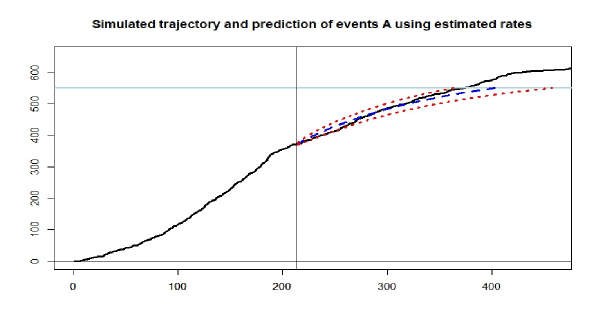
Figure 1: Plot of number of events against time (in days), following the timeline of a simulated trial. The simulated trajectory of events A is marked by the black solid line, the initial parameters: $a_{A}=0.8$, $b_{A}=182$, $a_{L}=0.6$, $b_{L}=2611$ and $r=0.2$. An interim analysis was taken at 7 months, the estimated parameters: $a_{A}=0.842$, $b_{A}=145$, $a_{L}=0.641$, $b_{L}=2697$ and $r=0.276$. Predictions on future event counts were created using the estimated parameters; the mean trajectory is shown by the blue dashed line, the 90% confidence bounds by the red dotted lines.

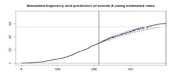
Figure 2: Plot of number of events against time (in days), following the timeline of a simulated trial. The simulated trajectory of events A is marked by the black solid line, the initial parameters: $a_{A}=1.2$, $b_{A}=213$, $a_{L}=1.4$, $b_{L}=3701$ and $r=0.2$. An interim analysis was taken at 7 months, the estimated parameters: $a_{A}=1.265$, $b_{A}=175$, $a_{L}=1.406$, $b_{L}=3916$ and $r=0.305$. Predictions on future event counts were created using the estimated parameters; the mean trajectory is shown by the blue dashed line, the 90% confidence bounds by the red dotted lines.

In both cases, the model successfully predicts the trajectory of the number of events $A$ with the real trajectory falling within the 90% predicted bounds. Furthermore, the parameters estimated at the cut-off time using maximum likelihood technique are close to the initial parameters showing an appropriate estimation.

6 Software development

In order to expose the event and recruitment prediction models (as detailed in the previous sections) to a large number of key stakeholders, an R package (EventPrediction) has been developed, tested and deployed to a centralised R server. The EventPrediction package allows a user to easily pass the data required (i.e. subject event data, centre level data and configuration) and return back key parameter estimates and predictions with bounds, for both events and recruitment.

6.1 R package design

R was chosen over other programming languages, and an R Package was developed over standalone R scripts, for a number of reasons, including: R has an easy to use and to setup testing framework; R ships with easy to use code coverage tools; R has a Comprehensive R Archive Network ("CRAN") set of packages that are easily accessible; R seamlessly integrates with GitLab (and other source control software); R allows for an Object Oriented ("OO") approach (i.e. S3, S4 and R6); and also, primarily, it is simply straightforward to develop, test, document and centrally deploy an R Package for key stakeholders to use.

R’s S3 lightweight OO solution was a key design feature of the EventPrediction package, as using such an OO approach yields four main benefits: first, S3’s simple to use OO benefit of polymorphism (aka in R as method dispatch); secondly, S3 gives the OO benefit of inheritance; thirdly, S3 is ubiquitously used by R contributors, easy to use and for others to comment; and fourthly, S3 is in accordance with the functional programming paradigm, when an object is passed into an S3 function it is not going to change (unlike full OO approaches like R6).

6.1.1 Good software engineering principles

Another major benefit of developing an R Package (and utilising R’s OO approach) is to ensure adherence to good Software Engineering principles, with code that is at a minimum: reliable; easy to use; efficient; well tested, with tests traceable to requirements and/or design; well documented; and (importantly) easy to maintain. The EventPrediction package conforms to each of these key programming elements, not only because these are simply good Software Engineering practices, but also as the biotechnology sector is highly regulated and there is a requirement to document a number of Software Development Life Cycle ("SDLC") tasks in accordance with departmental, company and regulatory policies.

6.1.2 R package SDLC and platform architecture

Before the design, development and/or testing of any code was initiated, two further key platform architectural design decisions were made: first, GitLab was used for source control, continuous integration, documentation, vignettes, readme files and also as part of the full deployment process; and secondly, R Studio Server Pro was used for development and testing of code, a Docker Image with a physical R server on AWS.

6.1.3 Further R package design: function layers

With a large number of complex R scripts and source papers another design choice (primarily, to make the code easier to use and easier to maintain) was grouping the code into four layers using R’s S3 OO approach. The four programming layers are as follows:

Layer One: Highest Level: Main Exposed Application Programming Interface (API).

This level is exposed to the user and contains: S3 Classes (functions) that allow instantiation of the objects that contain the input data required and configuration; functions to predict events and recruitment; plotting and printing functionality; and key getter functions.

Layer Two: Second Level Functions.

This level is not exposed to the user and is simply used to dispatch to the third level functions based on the S3 configuration objects instantiated in Layer One.

Layer Three: Third Level Functions.

This level is not exposed to the user and contains the main set of controller code and does all of the hard work of the package.

Layer Four: Lowest Level Functions.

This level is not exposed to the user and contains a large number of complex R scripts/algorithms that have been developed and tested using Monte Carlo Simulation, as detailed in the previous section.

6.2 R package input data required

The following set of input data is required by the EventPrediction package to predict events and recruitment (if recruitment is ongoing), with each set of data instantiated using R’s S3 approach (as detailed in the previous sections).

6.2.1 Event data

analysis_time_days	censor_flag	drop_out_flag	randomisation_date
28	0	0	YYYY-MM-DD
33	0	0	YYYY-MM-DD
87	1	0	YYYY-MM-DD
42	0	0	YYYY-MM-DD
77	1	1	YYYY-MM-DD

This data is in accordance with how the key stakeholders produce their data, it is transformed into the values as described in the previous sections, such that:

• analysis_time_days is the number of days from randomisation to either the event date ${T_{A}}$ or censoring date (i.e. the dropout date ${T_{L}}$ for subjects that have dropped out or the date used to censor at the cut off if a subject has not dropped out).

• censor_flag == 0 represents group A, a subject experienced event A.

• censor_flag == 1 & drop_out_flag == 0 represents group O, a subject did not experience an event nor dropout.

• drop_out_flag == 1 represents group L, a subject dropped out before the interim time.

6.2.2 Site recruitment data

study_centre_id	centre_actual_enrol	centre_recruitment_window_days
xx001	0	140
xx002	1	224
xx003	2	238
xx004	1	221
xx005	0	201

• centre_actual_enrol represents the number of subjects recruited at the unique centre ID.

• centre_recruitment_window_days represents the actual duration of recruitment at the unique centre ID (not including any screening period). The centre is active only during this interval $[a,b]$.

6.2.3 New Sites

A vector of days for new centres to be initiated {$u_{i}$}, e.g. $c(3,5,5,10,10,11,12,20)$.

6.2.4 Configuration

The following key pieces of information are accepted by the EventPrediction package (with appropriate defaults) which are used to select the appropriate algorithms and to provide key modelling values:

• distributions_to_use: A list detailing the distributions to model the dropouts and events: e.g. list(events = "Exponential", drop_outs = "Exponential")

• target_number_of_events: The target number of events for the analysis to be predicted

• sample_size: The number of patients planned to recruit

• confidence_level: The confidence probability for the upper and lower bounds

7 R package and implementation in a clinical trial

7.1 Introduction

In order to help the key stakeholders with the operational planning of a clinical trial and to test the quality of the prediction, the EventPrediction package was used on several historic studies. The following is one such case study in a historical oncology clinical trial, using the data at a given interim time when recruitment had not completed. The task was to predict the future recruitment and event counts with bounds and compare the results with the real trajectory of the recruitment and the events that have already occurred in the past.

The event and centre data was provided in accordance with the package API’s (as detailed in the previous section) along with a target number of events of 250 and patients sample size of 405. At the interim cut-off time the data for the study had the following recruitment and event status:

• 152 Events (i.e. censor_flag == 1)

• 155 At Risk (i.e. censor_flag == 1 and drop_out_flag == 0)

• 13 Drop Outs( i.e. drop_out_flag == 1)

• 85 patients left to recruit.

7.1.1 Key predictions

Given the above input and implementing the developed model, the EventPrediction package predicted:

Recruitment: Predicted number of days until target number of patients is reached with 90% bounds, (mean, lower bound, upper bound): 151, 120, 191.

The estimated parameters of a PG model are: $\alpha=4.8577,\beta=516.13$, and the prediction is constructed according to (15) where it was used some schedule of closing centres.

Events: Predicted number of days until target number of events reached, with 90% bounds, (mean, lower bound, upper bound):
exponential model: 227, 181, 322
Weibull model: 241, 188, 423

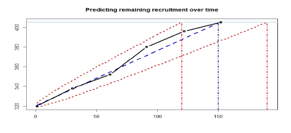
Figure 3: Prediction of the remaining recruitment against time from cut-off (in days). Real trajectory of patient recruitment is shown by black line. Mean prediction and 90% bounds are shown by the blue dashed and red dotted lines.

7.1.2 Plots and parameter estimates

Further, the EventPrediction package produced the following three key plots, along with key parameter estimates, for the key stakeholders to consume:
1) prediction of the remaining recruitment
2) prediction of the remaining number of events using exponential model
3) prediction of the remaining number of events using Weibull model

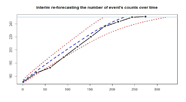
Figure 4: Prediction of the remaining number of events against time from cut-off (in days). Real trajectory of events is shown by black line. Exponential model, mean prediction and bounds depicted by the blue dashed and red dotted lines.

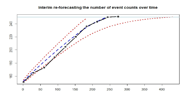
Figure 5: Prediction of the remaining number of events against time from cut-off (in days). Real trajectory of events is shown by black line. Weibull model, mean prediction and bounds depicted by the blue dashed and red dotted lines.

Fig 3 shows very good fit of the predictive area of recruitment where the real trajectory of the historical recruitment falls into the predictive area.

As one can see from Fig 4 and Fig 5, the predictions for both types of models, exponential and Weibull, are rather close, with the following estimated parameters for each:
Exponential model: $\mu_{A}=0.0069$, $\mu_{L}=0.00034$ and $r=0.2566$.
Weibull model: $a_{A}=1.1636$, $b_{A}=126.9995$, $a_{L}=0.3177$, $b_{L}=2053795.7$ and $r=0.2996$.

The actual number of days when the target number of patients was reached in this trial was 152 and the actual number of days when the planned number of events occurred is 244. As seen in the figures, the predictions were indeed very close to the actuals.

7.2 Predicting events when recruitment complete

We also considered the same case study as above, but at a later interim time when recruitment had completed. Therefore the task here was to predict the future event counts only.

As detailed in the previous section, this study has a target number of events of 250 and patients sample size of 405. At the interim cut-off time the data for the study had the following recruitment and event status:

• 220 Events (i.e. censor_flag == 1)

• 163 At Risk (i.e. censor_flag == 1 and drop_out_flag == 0)

• 22 Drop Outs( i.e. drop_out_flag == 1)

7.2.1 Key predictions

Given the above input and implementing the developed model, the EventPrediction package predicted:

Events: Predicted number of days until target number of events reached, with 90% bounds, (mean, lower bound, upper bound):
exponential model: 84, 60, 118
Weibull model: 83, 59, 116

7.2.2 Plots and parameter estimates

Further, the EventPrediction package produced the following two key plots, along with key parameter estimates, for the key stakeholders to consume:
1) prediction of the remaining number of events using exponential model
2) prediction of the remaining number of events using Weibull model

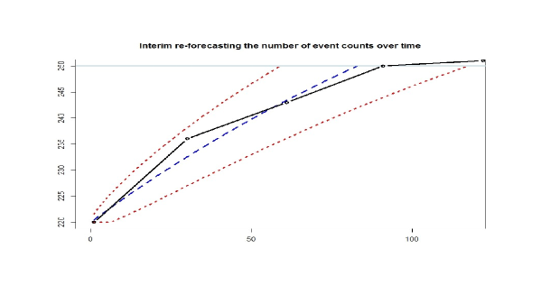
Figure 6: Prediction of the remaining number of events against time from cut-off (in days). Real trajectory of events is shown by black line. Exponential model, mean prediction and bounds depicted by the blue dashed and red dotted lines.

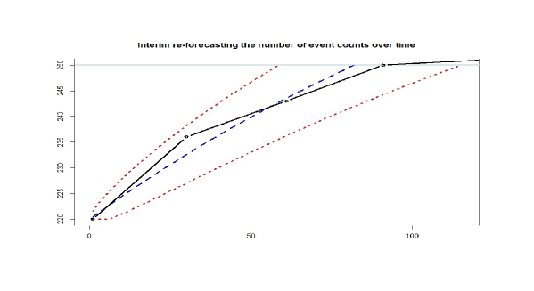
Figure 7: Prediction of the remaining number of events against time from cut-off (in days). Real trajectory of events is shown by black line. Weibull model, mean prediction and bounds depicted by the blue dashed and red dotted lines.

As one can see from Fig 6 and Fig 7, the predictions for both types of models, exponential and Weibull, are rather close, with the following estimated parameters for each:
Exponential model: $\mu_{A}=0.00553$, $\mu_{L}=0.00034$ and $r=0.2128$.
Weibull model: $a_{A}=0.9834$, $b_{A}=183.8473$, $a_{L}=0.36351$, $b_{L}=349763.5$ and $r=0.2067$.

The actual number of days when the planned number of events occurred is 91. As seen in the figures, the predictions were indeed very close to the actuals.

8 Fitting models to real data

8.1 Kaplan-Meier plots

To assess the model fit, we looked at the Kaplan-Meier (KM) curve for each interim dataset and compared these to the predicted survival functions for exponential and Weibull distributions. This provides a visualisation for model fit: the best fit model for the interim data will be the model which distribution best maps the KM curve. This is for the occurrence of events $A$ and so will only inform of the best distribution for modelling events $A$. However, similar curves can be created to test the fit of dropout distribution.

The survival functions for exponential and Weibull models with cure are calculated using their respective estimated parameters, with formulae:

Exponential: $S(x,r,\mu_{A})=r+(1-r)\exp(-\mu_{A}x)$
Weibull: $S(x,r,\alpha_{A},b_{A})=r+(1-r)\exp(-(\frac{x}{b_{A}})^{\alpha_{A}})$

In Fig 8, one can see that the predicted survival functions for exponential and Weibull models are very close and both map the KM curve well.

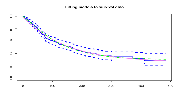
Figure 8: Kaplan-Meier plot showing survival function using interim data with associated confidence intervals (blue lines), alongside survival functions for exponential (violet solid line) and Weibull (green dashed line) cure models.

8.2 AIC and BIC criteria

We also used Akaike information criterion (AIC) and Bayesian information criterion (BIC) to test which model best fits the real dataset. These are calculated by:

AIC $=2k-2{\rm LogLik}$

BIC $=k\log(n)-2{\rm LogLik}$

where $k$ = number of parameters in the model, $n$ = total number of patients at interim time, ${\rm LogLik}$ = the log-likelihood from parameter estimation.

For the stopped recruitment case:

Model	AIC	BIC
Exponential model, no cure	3333.6	3341.6
Exponential cure model	3319.0	3327.1
Weibull (A) and exponential (L) cure model	3321.0	3333.0
Exponential (A) and Weibull (L) cure model	3283.1	3299.1
Weibull cure model	3285.0	3305.1

For the ongoing recruitment case:

Model	AIC	BIC
Exponential model, no cure	2222.9	2230.4
Exponential cure model	2210.9	2218.4
Weibull (A) and exponential (L) cure model	2209.3	2220.6
Exponential (A) and Weibull (L) cure model	2183.7	2198.7
Weibull cure model	2182.1	2200.9

The lower the AIC or BIC, the better the model fit. From the two tables above, one can see that the cure models show an improvement on the ”no cure” model. The exponential (A) and Weibull (L) cure model is the best fit for the stopped recruitment dataset. By small margins, the values of criteria for ongoing recruitment suggest either the Weibull cure model or the exponential (A) and Weibull (L) cure model is best suited for the data.

Conclusions

We have developed a new analytic approach for the prediction of event counts in event-driven trials when recruitment is complete or ongoing. We use the exponential and Weibull models and account for patient dropout and opportunity of cure. Not only can we predict the future occurrence of events, but we can also predict any remaining recruitment, with mean and bounds, using the Poisson-gamma recruitment model. The developed results can be easily extended to the combined cure models using the combination of exponential and Weibull distributions for the time to event and the time to dropout and also to log-normal with cure model.

Using these novel advanced models and with access to real subject level and centre level data we are now able to address key business use cases for a number of key stakeholders in order to better forecast the operational design of event-driven clinical trials. Furthermore, by centralising an exposed R Package EventPrediction, utilising good software engineering principles, each of our key stakeholders have access to the package and can obtain plots, parameter estimates and predictions with bounds, without contacting the mathematical modellers nor the R package developer.

We have many opportunities for future improvements to the mathematical modelling and EventPrediction package. One of the major priorities is to evaluate the predictions against real clinical trial operational data to ensure the existing and any future models are as accurate as we found in testing on historical data. We are also looking to incorporate other statistical distributions for modelling time to both the main event and dropout.

References

- [1] V. Anisimov and V. Fedorov. Modeling, prediction and adaptive adjustment of recruitment in multicentre trials, Statistics in Medicine, 26, 27, 4958–4975, 2007.
- [2] V. Anisimov, D. Downing and V. Fedorov. Recruitment in multicentre trials: prediction and adjustment, mODa 8 - Advances in Model-Oriented Design and Analysis, 1–8, 2007.
- [3] V. Anisimov. Using mixed Poisson models in patient recruitment, Proc. of the World Congress on Engineering, II, 1046–1049, 2008.
- [4] V. Anisimov. Statistical modeling of clinical trials (recruitment and randomization), Communications in Statistics - Theory and Methods, 40, 19-20, 3684–3699, 2011.
- [5] V. Anisimov. Predictive event modelling in multicentre clinical trials with waiting time to response, Pharmaceutical Statistics, 10, 6, 517–522, 2011.
- [6] V. Anisimov. Predictive hierarchic modelling of operational characteristics in clinical trials, Communications in Statistics - Simulation and Computation, 45, 5, 1477–1488, 2016.
- [7] V. Anisimov. Discussion on the paper "Real-time prediction of clinical trial enrollment and event counts: a review" by D.F. Heitjan et al. Contemporary Clinical Trials, 40, 7–10, 2016.
- [8] V. Anisimov. Modern analytic techniques for predictive modelling of clinical trial operations, Quantitative Methods in Pharmaceutical Research and Development: Concepts and Applications, Springer International Publ., 361–408, 2020.
- [9] V. Anisimov and M. Austin. Centralized statistical monitoring of clinical trial enrollment performance, Communications in Statistics - Case Studies and Data Analysis, 6, 4, 2020, 392–410.
- [10] E. Bagiella and D.F. Heitjan. Predicting analysis times in randomized clinical trials, Statistics in Medicine, 20, 2055–2063, 2001.
- [11] K.D. Barnard, L. Dent and A. Cook. A systematic review of models to predict recruitment to multicentre clinical trials, BMC Medical Research Methodology, 10, 63, 2010.
- [12] J.M. Bernardo and A.F.M. Smith. Bayesian Theory, John Wiley & Sons: Hoboken, NJ, USA, 2004.
- [13] T.T. Chen. Predicting analysis times in randomized clinical trials with cancer immunotherapy, BMC medical research methodology, 16(1), 1–10, 2016.
- [14] E. Gkioni, R. Riusd, S. Dodda and C. Gamblea. A systematic review describes models for recruitment prediction at the design stage of a clinical trial, Journal of Clinical Epidemiology, 115:141–149, 2019.
- [15] D.F. Heitjan, Z. Ge and G.S. Ying. Real-time prediction of clinical trial enrollment and event counts: a review, Contemporary Clinical Trials, 45, part A, 26–33, 2015.
- [16] R.E. Carter, S.C. Sonne and K.T. Brady. Practical considerations for estimating clinical trial accrual periods: Application to a multi-center effectiveness study, BMC Medical Research Methodology 5:11–15, 2005.
- [17] S. Senn. Statistical Issues in Drug Development. Wiley: Chichester, 1997.
- [18] S. Senn. Some controversies in planning and analysis multi-center trials. Statistics in Medicine, 17, 1753–1756, 1998.