Boosting of Head Pose Estimation by Knowledge Distillation

Abstract

We propose a response-based method of knowledge distillation (KD) for the head pose estimation problem. A student model trained by the proposed KD achieves results better than a teacher model, which is atypical for the response-based method. Our method consists of two stages. In the first stage, we trained the base neural network (NN), which has one regression head and four regression via classification (RvC) heads. We build the convolutional ensemble over the base NN using offsets of face bounding boxes over a regular grid. In the second stage, we perform KD from the convolutional ensemble into the final NN with one RvC head. The KD improves the results by an average of 7.7% compared to base NN. This feature makes it possible to use KD as a booster and effectively train deeper NNs. NNs trained by our KD method partially improved the state-of-the-art results. KD-ResNet152 has the best results, and KD-ResNet18 has a better result on the AFLW2000 dataset than any previous method. We have made publicly available trained NNs and face bounding boxes for the 300W-LP, AFLW, AFLW2000, and BIWI datasets. Our method potentially can be effective for other regression problems.

1 Introduction

Facial analysis is one of the most important tasks of computer vision. This includes such tasks as face detection [1], facial landmarks detection [2], facial age estimation [3], head pose estimation (HPE) [4], and others [5]. In this paper, we focus on HPE. Many practical applications, such as analyzing facial expressions [6], gaze estimation [7], and others [8, 9], require fairly accurate HPE.

The head pose is usually a vector containing the pitch, yaw, and roll angles. This vector is visualized using three axes, as shown in Fig. 1. The HPE problem is to find these angles from the image of the face.

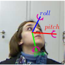
Figure 1: Visualization of head pose.

Many approaches have been proposed to solve the HPE problem. One of the first approaches was to use appearance template methods [10], deformable models [11], manifest embeddings methods [12], facial landmarks [13, 14], and others [15, 16]. An overview of these methods is given in  [4, 17]. Recently, convolutional neural networks (NNs) have been widely used to solve many computer vision problems. Applying this approach to the HPE problem yields good results [17].

A typical workflow for the HPE problem based on NN contains several consecutive operations. First, the detector finds a bounding box around the face. Next, the image is cropped according to the found bounding box and resized. After that, a specialized NN estimates the head pose from the cropped image.

To improve the HPE quality of NNs, researchers have developed various methods to encode angles [18, 19, 20], configurations of head branches [19, 21, 22], and loss functions [23, 21, 24]. However, the datasets used in the test protocols have low representativeness. We have demonstrated that simple NN trained using rotation augmentation is close to the state-of-the-art (SOTA) result of complex NN [25]. In this paper, we propose an advanced augmentation workflow and a NN architecture with one regression head and four RvC heads to improve HPE accuracy.

One way to additionally improve prediction accuracy is to train several NNs and then use an ensemble of their predictions [26, 27]. The disadvantage of this approach is the increase in the computational complexity of the prediction since it is necessary to get predictions from all the NNs. The knowledge distillation (KD) method was proposed [28, 29] to solve this problem. The essence of this method is to train a new NN using the trained NNs. This method has been used in several studies and has yielded good results [30].

A simple and popular way of KD is the response-based method, which trains the student to repeat the teacher response. A student trained by the response-based method always has results worse than the teacher model for the classification problem [30, 31, 32, 33]. For the regression problem, response-based methods are ineffective for NN with a naive regression head. The naive regression head response does not contain dark knowledge. It is more efficient to train NN without a teacher.

In [34], Shao et al. demonstrate that the bounding box significantly affects the quality of the trained NN for the HPE problem. In [35], Shao et al. propose an approach in which the bounding box is first corrected, and then the angles are predicted using the NN from [18].

We have developed a convolutional ensemble that uses this feature of bounding boxes. The proposed ensemble forms an image batch by shifting the original bounding box over the regular grid and cropping the image for each shifted bounding box. The ensemble prediction is the averaged NN predictions of obtained image batch. We used KD from the convolutional ensemble to reduce computational costs. Unexpectedly, NN trained using KD boosted the ensemble accuracy of HPE. At the same time, KD has not yet been used for HPE.

This paper makes the following contributions.

• We propose a preprocessing workflow and a NN architecture with one regression head and four RvC heads. Trained NN improves the results of many previous HPE works.

• We propose a convolutional ensemble that makes multiple image cropping by shifting the original bounding box. The ensemble improves the NN results.

• We propose the KD method for the regression problem using RvC head and classification KD loss. NN trained with the proposed KD workflow boosts the convolutional ensemble accuracy and surpasses results on large datasets of previous HPE works.

2 Related work

This section gives an overview of the approaches used to solve the HPE problem. Subsection 2.1 provides an overview of methods based on facial landmarks. Subsection 2.2 describes an overview of landmark-free methods. Subsection 2.3 contains a KD methods overview.

2.1 Landmark-based methods

Initially, facial landmark approaches were used for HPE. Such methods first find facial landmarks in the image, using, for example, the algorithm from [2]. Then the head pose is estimated using the average 3D head model and some algorithm [36, 37]. Some methods, such as [38], use a depth map as additional information. The applicability of these methods is limited by the need to use special devices to obtain RGB-D images.

However, these methods significantly depend on finding facial landmarks. In some cases, facial landmarks are difficult to find accurately. For example, when part of the face is hidden. One way to solve this problem could be to use heat maps of facial landmarks [39]. Also, the RANSAC [40] algorithm can be used, or an incomplete set [41] of facial landmarks can be used. Another problem with these methods is using an averaged 3D head model. The difference between the actual 3D head model and the average 3D head model introduces an additional error in the estimation. In [42], Yuan et al. suggest solving this problem by using four facial landmarks and a 3D head model morphing with spherical parametrization. However, close to the SOTA results are obtained only using depth information.

2.2 Landmark-free methods

In [43, 44, 45], the possibility of solving the HPE problem using convolutional NNs without using key points is demonstrated. These approaches yield better results than approaches based on facial landmarks. Also, these methods are less susceptible to the problems associated with overlapping parts of the face, and they do not depend on the accuracy of finding facial landmarks.

HopeNet [23] is one of the first methods to yield good results. The final prediction of the angles was calculated using RvC [46] with a bin size of 3. The loss function in this method combined classification and regression loss functions. Subsequently, this approach received several improvements. In [21], Wang et al. present a modification of this method, in which the final prediction used an RvC head with a bin size of 1, and other RvC heads with bigger bin sizes were used as regularizers during the training. In [47], Huang et al. present another modification of the method. This modification also uses an RvC head, but the top 40 classes were used for the HPE. Some researchers [48, 49] use depth maps as additional information. Although these studies have obtained good results, the practical applicability of these methods is also limited by the availability of special cameras.

One of the recent works [50] has results that surpass all previous results. Valle et al. in [50] extend the training dataset with head poses by a dataset with facial landmarks. Authors train the NN to localize facial landmarks and estimate head pose. The facial landmarks act as a regularizer. The expansion of the dataset could significantly improve the representativeness of the data and lead to improving metrics for the HPE problem.

2.3 Knowledge distillation methods

Large deep NNs demonstrate excellent results on tasks with a large training sample. Over parameterization provides fine-tuning, which improves quality metrics in most tasks [51, 52]. However, large NNs are difficult to use on mobile devices and embedded systems due to limited computing resources. In some cases, small NNs trained from scratch may not provide the required quality. This problem can be solved by various methods: quantization [53], pruning [54], KD [33]. Quantization and pruning compress a large model, and KD trains a small student model using large teacher model predictions. In most cases, these methods can be used together. A flexible training scheme of KD allows one to customize it for different scenarios.

The KD method originates in [31]. Bucilua et al. in [31] proposed a method of training a small model using the predictions of a large model or an ensemble of models. Later, Hinton et al. in [33] formally popularized this method as KD.

Initially, KD was used for a classification problem. The predicted probability distribution of classes is the dark knowledge of the teacher model, which helps to train the student model. This distillation method is called response-based since the student model tries to repeat the teacher model responses completely. The response-based method allows using ensembles as a teacher without additional improvements. However, using this method, the student always has worse results than the teacher for a classification problem [30, 31, 32, 33].

However, using the response-based method in many tasks does not positively affect. For such tasks, the feature-based method trains the student model to predict the same features maps as the teacher model on the intermediate layers. The feature-based method does not allow using ensembles as a teacher without additional adapter layers [55]. In some cases, the feature-based method allows the student model to improve the result of the teacher model [56, 57].

The response-based method of KD has not been used for the regression problem. In most cases, naive coding is used, in which a single neuron predicts continuous values from a given range. This coding does not allow the teacher model to provide unique dark knowledge. Using the RvC heads allows one to adapt the response-based method to the regression problem. Initially, the response-based method was developed for the classification problem. The KD scheme using RvC heads has not been used before for the regression problem.

3 Method

In this paper, we propose a neural network training method by KD from a convolutional ensemble for the HPE problem. First, we formulate the HPE problem in subsection 3.1. Then, we describe the architectures of the trained NN in subsection 3.2.

Getting the final NN is done in two stages. In the first stage, we train an NN to perform the HPE. We construct a convolutional ensemble based on the trained NN model and offsets of the bounding box. The algorithm is given in subsection 3.3. In the second stage, we train the final NN. The training uses the results of the prediction of the constructed convolutional ensemble. A detailed description of the KD is given in subsection 3.4.

3.1 Problem formulation

The HPE problem is to use an image of a face to predict the pitch, yaw, and roll angles of that face. Consider the images $\mathcal{X}=\left\{X_{1},\dots,X_{N}\right\}$ and the pose vector $\vec{y}_{k}~{}=~{}\left(\alpha_{k},\beta_{k},\gamma_{k}\right)$ for each image $X_{k}$, where $N$ is the number of images, while $\alpha_{k}$, $\beta_{k}$, $\gamma_{k}\in\left[-\theta;\theta\right]$ represent the pitch, yaw, and roll angles, respectively. The goal is to find a function $\mathcal{F}$ that estimates the head pose for the image $X$, minimizing the mean average error (1).

$$E\left(\mathcal{X}\right)=\frac{1}{N}\sum_{i=1}^{N}\|\mathcal{F}\left(X_{i}\right)-\vec{y}_{i}\|_{1}$$ (1)

3.2 Architecture of the neural network

Our proposed architecture consists of a backbone and several head branches. We use a NN from the ResNet family [58] as a backbone. At the first stage of training, we use head branches consisting of one regression head and four RvC heads with bin sizes: 1, 2, 3, 4. In the second stage of training, we use a single head branch, an RvC head with a bin size of 1. The NN architecture is shown in Fig. 2.

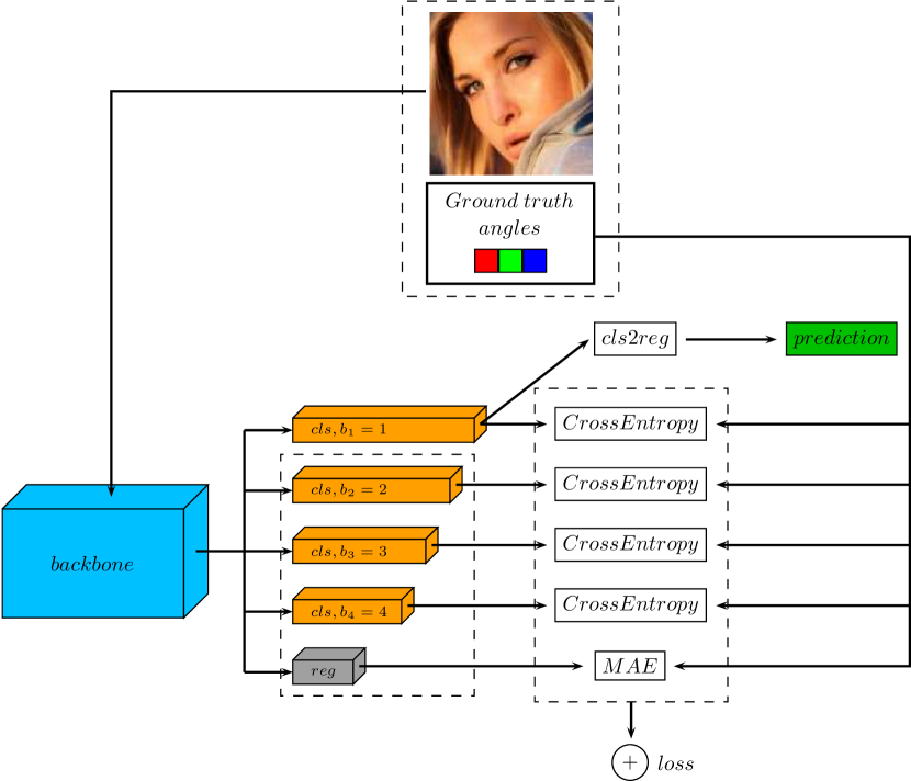
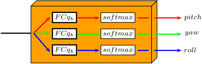
(a) classification head (cls)

(b) regression head (reg)

Figure 2: Architecture of the neural network. ResNet* is used as a backbone. The NN has one regression head, and four RvC heads with bin sizes: 1, 2, 3, 4. The RvC head with bin size 1 is used for prediction. Other heads are used as regulators during the training. In the first stage, all heads are used. In the second stage, the regulatory heads are removed.

Previous research [23, 21, 34, 47] used ResNet50 as a backbone. The experiments section demonstrates that deeper ResNet101 and ResNet152 models do not significantly improve accuracy with single-stage training. This result justifies the choice of ResNet50 as a backbone earlier. However, our two-stage training allows one to improve accuracy by using more deeper models.

The proposed head branches configuration has not been used before. Ruiz et al. in [23] used one RvC head with joint classification/regression loss. Wang et al. in [22] used several RvC heads with different sizes of bins. The authors used joint classification/regression loss for the head with the smallest bin size. Hsu et al. in [19] used one regression head and one RvC head, which worked in ranking mode. We found that the configuration with one regression head and four RvC heads provides the best quality. At the same time, removing any of them leads to a drop in quality during training at the first stage. At the second stage of training, one RvC head with a bin size equal to one is enough. We also noticed that using joint classification/regression loss for RvC heads does not improve quality. This result may be caused by augmentations, which significantly increased the representativeness of the training sample. We demonstrated [25] that a single RvC head NN trained using rotation augmentation achieves results close to SOTA.

Below we provide a formal description of the heads in a generalized form. In the first stage, the NN contains several head branches: $M$ fully connected layers that perform the classification with bin sizes $B=\left\{b_{1},\dots,b_{M}\right\}$, number of bins $Q=\left\{q_{1},\dots,q_{M}\right\}$, and a fully connected layer performing a regression. In the second stage, the NN contains only one head branch: a fully connected layer that performs a classification with the bin size $b_{k}\in B$.

Here we describe the method for making the NN predictions during the training for the proposed architecture. For a classification head with bin size $b_{k}$ and number of bins $q_{k}$, the angles are calculated using the formula (2), where $\vec{c}=\left(c_{1},\dots,c_{q_{k}}\right)\in{\left[-\theta;\theta\right]}^{q_{k}}$ is the bin center vector, and $\vec{y\,}_{\textup{out}}^{\left(k\right)}=\left(\vec{\alpha\,}_{out}^{\left(k\right)},\vec{\beta\,}_{\textup{out}}^{\left(k\right)},\vec{\gamma\,}_{\textup{out}}^{\left(k\right)}\right)\in\mathbb{R}^{q_{k}\times 3}$ is the output of the $k$th classification head. For a regression head, the angles are calculated using the formula (3), where $\vec{y\,}_{\textup{out}}^{\textup{reg}}=\left(\alpha_{\textup{out}}^{\textup{reg}},\beta_{\textup{out}}^{\textup{reg}},\gamma_{\textup{out}}^{\textup{reg}}\right)\in\mathbb{R}^{3}$ is the output of the regression head.

$$\xi_{\textup{pred}}^{\left(k\right)}=\langle\vec{c\,},\operatorname{softmax}\left(\vec{\xi\,}_{\textup{out}}^{\left(k\right)}\right)\rangle \text{where}~{}\xi\in\left\{\alpha,\beta,\gamma\right\}$$ (2)

$$\xi_{\textup{pred}}^{\textup{reg}}=\theta\tanh\left(\xi_{\textup{out}}^{\textup{reg}}\right) \text{where}~{}\xi\in\left\{\alpha,\beta,\gamma\right\}$$ (3)

The resulting loss function is the averaging of the loss functions of all heads. The resulting loss function $\mathcal{L}$ is calculated using the formulas (4), where for some image $\vec{y}_{\textup{gt}}=\left(\alpha_{\textup{gt}},\beta_{\textup{gt}},\gamma_{\textup{gt}}\right)$ is the ground truth pose vector, $\vec{y\,}_{\textup{out}}^{\left(j\right)}=\left(\vec{\alpha\,}_{\textup{out}}^{\left(j\right)},\vec{\beta\,}_{\textup{out}}^{\left(j\right)},\vec{\gamma\,}_{\textup{out}}^{\left(j\right)}\right)$ is the output of the $k$th classification head, and $\vec{y\,}_{\textup{pred}}^{\textup{reg}}=\left(\alpha_{\textup{pred}}^{\textup{reg}},\beta_{\textup{pred}}^{\textup{reg}},\gamma_{\textup{pred}}^{\textup{reg}}\right)$ is the output of the regression head.

$$\begin{gathered}\mathcal{L}^{\left(j\right)}\left(\vec{y}_{\textup{gt}},\vec{y\,}_{\textup{out}}^{\left(j\right)}\right)=\sum_{\xi\in\left\{\alpha,\beta,\gamma\right\}}\operatorname{CrossEntropy}\left(\xi_{\textup{gt}},\vec{\xi\,}_{\textup{out}}^{\left(j\right)}\right)\\ \mathcal{L}^{\textup{reg}}\left(\vec{y}_{\textup{gt}},\vec{y\,}_{\textup{pred}}^{\textup{reg}}\right)=\operatorname{MAE}\left(\vec{y}_{\textup{gt}},\vec{y\,}_{\textup{pred}}^{\textup{reg}}\right)\\ \mathcal{L}=\frac{\mathcal{L}^{\textup{reg}}\left(\vec{y}_{\textup{gt}},\vec{y\,}_{\textup{pred}}^{\textup{reg}}\right)+\sum_{j=1}^{M}\mathcal{L}^{\left(j\right)}\left(\vec{y}_{\textup{gt}},\vec{y\,}_{\textup{out}}^{\left(j\right)}\right)}{M+1}\end{gathered}$$ (4)

The output of a fully connected classification layer with a minimum bin size $b_{k}$ is used to calculate the NN prediction in test mode. The remaining heads are used as regularizers during training.

3.3 Convolutional ensemble

In [59], Dietterich demonstrates that one of the easiest ways to improve the accuracy of machine learning algorithms is to use an ensemble. This method consists of training several models and then averaging their predictions. Note that the choice of bounding box affects the prediction result [34, 35].

Based on these facts, we decided to use the predictions of the single NN, but with different face bounding box offsets.

Initially, we trained the NN to obtain quasi-ensemble predictions for different offsets of the bounding box. For a NN, we implemented a quasi-ensemble by expanding the input image. Suppose that a NN is a convolution with a $224\!\times\!224$ kernel. Then it returns a $1\!\times\!1$ prediction of angles for an image with a resolution of $224\!\times\!224$. For an image with a resolution of $226\!\times\!226$, the NN returns $3\!\times\!3$ predictions, which then are averaged by a quasi-ensemble. It is necessary to increase the bounding box proportionally to increase the input image resolution because the input image is obtained by cropping the dataset image along a bounding box. However, the HPE accuracy of the quasi-ensemble decreased by more than 10% compared to the variant without image extension. The NN does not receive critical information about the image borders in a quasi-ensemble. The padding function in the NN denotes borders with zeros. However, cropping images for each bounding box offset and independent prediction by the NN increases the HPE accuracy due to averaging. We call this variant the convolutional ensemble because the bounding box offsets are carried out on a regular grid as a convolution. However, the NN predicts head pose independently for each offset. The convolutional ensemble is shown in Fig. 3.

Figure 3: Convolutional ensemble. The ensemble forms an image batch by shifting the original bounding box over the regular grid. The red box indicates the original bounding box, the green box indicates shifted bounding box. The dimensions of the bounding box remain the same during offset. The NN predicts head poses for the batch. The final result of the ensemble prediction is the average result for the batch.

Figure 4: Knowledge distillation workflow. The left part contains the teacher model – the convolutional ensemble that estimates the head pose from the input image. The right part contains the student model – the NN with one RvC head, which bin size is 1. The student model is trained on the teacher model predictions and labeling from the dataset.

The convolutional ensemble is based on a trained NN described in section 3.2. The NN has four RvC heads and one regression head. The convolutional ensemble predicts angles from the prepared image, cropped by edges and resized to the required size. The resulting image is the receptive field of the ensemble. Then, we calculate a set of NN predictions using the resulting image and a set of bounding box offsets. The final prediction of the ensemble is the average value over the prediction set.

Consider the mathematical formalization of a convolutional ensemble. Let introduce the following notation. Let $s\!\in\!\mathbb{N}$ and $p\!\in\!\left\{0,s,2s,...\right\}$ be the parameters of the ensemble, where $s$ is stride and $p$ is padding, and the input image of the NN has dimensions $C\!\times\!h\!\times\!w$. It is necessary to apply a convolutional ensemble for a dataset image $X\!\in\!\mathbb{R}^{C\!\times\!H\!\times\!W}$ with a bounding box having coordinates $\left(x_{1},y_{1},x_{2},y_{2}\right)$.

Let’s calculate the scaling parameters of a dataset image using the formulas: $r_{x}=\frac{w}{x_{2}-x_{1}}$ and $r_{y}=\frac{h}{y_{2}-y_{1}}$. Then, we scale the dataset image with the coefficients $\left(r_{x},r_{y}\right)$. Then we crop the scaled image by $\left(x_{1}r_{x}\!-\!p,y_{1}r_{y}\!-\!p,x_{2}r_{x}\!+\!p,y_{2}r_{y}\!+\!p\right)$. As a result, we get an input image $Z\!\in\!\mathbb{R}^{C\!\times\!\left(h\!+\!2p\right)\!\times\!\left(w\!+\!2p\right)}$ for the convolutional ensemble. Note that at this stage we have already applied the padding function, taking the missing values from the dataset image.

Next, we calculate the set of offsets coordinates $\mathcal{B}_{s,p}\left(w,h\right)$ by (5) using convolutional ensemble parameters $s$ and $p$.

$$\mathcal{R}_{i,j}^{\left(s\right)}\!\left(w,h\right) =\left(si,sj,si+w,sj+h\right)$$ (5)

$$\mathcal{B}_{s,p}\left(w,h\right) =\left\{\mathcal{R}_{i,j}^{\left(s\right)}\!\left(w,h\right)\colon\!\left(0\!\leq\!i,j\!\leq\!2\frac{p}{s}\right)\!\land\!\left(i,j\!\in\!\mathbb{Z}\right)\right\}$$

For each $b\in\mathcal{B}_{s,p}\left(w,h\right)$, we crop the image $Z$ by $b$ and calculate the predictions of the NN. As the result we get $A=\left(2\frac{p}{s}+1\right)^{2}$ predictions. Next, we calculate the final prediction of the convolutional ensemble using formula (6). Note that in this formula, the result is probabilities.

$$\xi_{\textup{ens}}^{\left(j\right)} =\frac{1}{A}\sum_{i=1}^{A}\left(\operatorname{softmax}\left(\vec{\xi\,}_{\textup{out}}^{\left(i\right)}\right)\right)_{j}, \xi\in\left\{\alpha,\beta,\gamma\right\}$$ (6)

$$\vec{\xi}_{\textup{ens}} =\left(\xi_{\textup{ens}}^{\left(1\right)},\dots,\xi_{\textup{ens}}^{\left(q_{k}\right)}\right), \xi\in\left\{\alpha,\beta,\gamma\right\}$$

3.4 Knowledge distillation

The convolutional ensemble uses multiple NN predictions for a single image. On the one hand, this increases the accuracy of prediction, but on the other hand, it increases the number of calculations by orders of magnitude. Additional calculations reduce the performance and practical applicability of the convolutional ensemble. We applied the KD method to neutralize the decreasing performance.

The KD method train the student model to repeat the teacher model response. A student trained by the response-based method always has results worse than the teacher model for the classification problem [30, 31, 32, 33]. For naive regression, the response-based method is useless. In our case, the student model is superior to the teacher model. As a teacher model, we used a convolutional ensemble. As a student model, we used a NN with a single head branch, which is an RvC head with a bin size of 1. We train the NN using the KD method [28, 60], which is used for the classification problem. The KD workflow is shown in Fig. 4.

The loss function for KD is calculated using (7), where $D_{\textup{KL}}$ is the Kullback–Leibler divergence [61], for some image $\vec{y}_{\textup{gt}}=\left(\alpha_{\textup{gt}},\beta_{\textup{gt}},\gamma_{\textup{gt}}\right)$ is the ground truth pose vector, $\vec{y}_{\textup{out}}=\left(\vec{\alpha}_{\textup{out}},\vec{\beta}_{\textup{out}},\vec{\gamma}_{\textup{out}}\right)$ is the output of the trained NN, and $\vec{y}_{\textup{ens}}=\left(\vec{\alpha}_{\textup{ens}},\vec{\beta}_{\textup{ens}},\vec{\gamma}_{\textup{ens}}\right)$ is the prediction of the convolutional ensemble, calculated using (6).

$$\begin{gathered}\mathcal{L}_{\textup{cls}}\left(\vec{y}_{\textup{gt}},\vec{y}_{\textup{out}}\right)=\sum_{\xi\in\left\{\alpha,\beta,\gamma\right\}}\operatorname{CrossEntropy}\left(\xi_{\textup{gt}},\vec{\xi}_{\textup{out}}\right)\\ \mathcal{L}_{\textup{dist}}\left(\vec{y}_{\textup{ens}},\vec{y}_{\textup{out}}\right)=\sum_{\xi\in\left\{\alpha,\beta,\gamma\right\}}D_{\textup{KL}}\left(\vec{\xi}_{\textup{ens}}\|\vec{\xi}_{\textup{out}}\right)\\ \mathcal{L}=\frac{0.05\cdot\mathcal{L}_{\textup{cls}}\left(\vec{y}_{\textup{gt}},\vec{y}_{\textup{out}}\right)+\mathcal{L}_{\textup{dist}}\left(\vec{y}_{\textup{ens}},\vec{y}_{\textup{out}}\right)}{2}\end{gathered}$$ (7)

The prediction is calculated using the following formulas (2). Note also that at this stage, we can choose a different backbone from the one used in the first stage.

4 Datasets

In this section, we describe the datasets used in the experiments. Subsection 4.1 provides an overview of the datasets used. Subsection 4.2 describes the data preprocessing. Subsection 4.3 contains a list of the augmentations used. Lastly, subsection 4.4 describes the test protocols used for the HPE.

4.1 Description

Research on HPE usually uses the datasets 300W-LP [13], AFLW2000 [13], AFLW [62], and BIWI [63]. 300W-LP is synthetically generated using deformations of a 3D face model from AFW [64], LFPW [65], HELEN [66], and IBUG [67]. These datasets contain 2414 in-the-wild images with 3837 faces. 300W-LP contains 122450 images. AFLW contains 21120 images gathered from Flickr. AFLW2000 contains the first 2000 images from the AFLW dataset. BIWI contains 15677 images from 24 videos of 20 people obtained in a laboratory using Kinect. Note that BIWI, unlike the others, does not contain bounding boxes. Examples of dataset images are shown in Fig. 5.

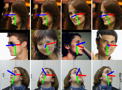
Figure 5: Examples of dataset images. The first line contains examples from 300W-LP, the second line contains examples from AFLW2000, and the third line contains examples from BIWI.

4.2 Preprocessing

We reduced the datasets following [23, 18, 21, 47, 24], leaving only images with head rotation angles in the range $\left[-99^{\circ};+99^{\circ}\right]$.

The images from the datasets contain a face and some background. The main object of analysis in the HPE problem is the face. Therefore, it is necessary to draw the attention of the NN to it. The attention mechanism is performed by cropping the image on the bounding box containing the face and further resizing it to the size of the NN.

The bounding boxes of 300W-LP, AFLW2000, and AFLW are obtained by constructing a bounding rectangle around the facial landmarks and then slightly enlarging them. BIWI does not contain bounding boxes. In the literature on HPE, bounding boxes are obtained in different ways. For example, the Faster R-CNN [68] detector was used in [23], the MTCNN [69] detector was used in [18], the Dlib [70] detector was used in [24, 47], and the depth maps were used in [50].

Since bounding boxes affect the result [34, 35], the differences in the ways of getting the bounding boxes do not allow for a valid comparison of the methods for HPE. We trained the YOLOv5 [71] detector on the WIDER [72] dataset to solve this problem We redefined the bounding boxes using this detector for all four datasets: 300W-LP, AFLW2000, AFLW, and BIWI. The new bounding boxes for these datasets are publicly available in [73], which will allow performing an objective comparison of methods for the HPE problem without depending on the bounding boxes.

4.3 Augmentations

Data augmentation is an integral part of NN training. Augmentation can significantly expand the training set and increase the representativeness of the data. Due to augmentation, it is possible to significantly improve the quality of the trained NN [74, 75].

Concerning the HPE problem, augmentation can be divided into two types: those that affect the head pose and those that do not affect the head pose. In our workflow, augmentations that affect the head pose are applied first, and then augmentations that do not affect the head pose.

We use a horizontal flip with a probability of $0.5$ and rotate by a random angle in the range $\left[-15^{\circ};+15^{\circ}\right]$ from the augmentations affecting the head pose. In the process of applying these augmentations, the head poses are corrected, as described in [25].

The augmentations that do not affect the head pose were taken from the Albumentations library [76]. First, with a probability of $0.5$, no augmentation is applied, or with a probability of $0.5$, one randomly selected augmentation from the list is applied: HueSaturationValue, CLAHE, Equalize, or Solarize. Then, with a probability of $0.5$, no augmentation is applied, or with a probability of $0.5$, one randomly selected augmentation from the list is applied: ChannelShuffle or ChannelDropout. Then MedianBlur is applied with a probability of $0.5$. Then, with a probability of $0.5$, no augmentation is applied, or with a probability of $0.5$, one randomly selected augmentation from the list is applied: RandomShadow or ISONoise. Lastly, CoarseDropout is applied with a probability of $0.5$.

4.4 Testing protocols

Following previous works, we use the following test protocols, shown in Table I. The test protocols are described in more detail below.

TABLE I: Test protocols

Protocol	Train		Test
	Dataset	# of Faces	Dataset	# of Faces
Protocol #1	300W-LP	$122415$	AFLW2000	1969
			BIWI	$15677$
Protocol #2	AFLW	$22079$	AFLW	$1969$
Protocol #3	BIWI	$10612$	BIWI	$5065$

Test protocol 1. 300W-LP is used for training, AFLW2000 and BIWI are used for testing. Only images from datasets with head rotation angles in the range $\left[-99^{\circ};+99^{\circ}\right]$ were used.

Test protocol 2. AFLW is used for training and testing. In [77], Amador et al. point out no standard test protocol for AFLW. In addition, some researchers [14, 21] use a random division of the dataset into training and testing. It does not allow for a valid comparison of methods. For these reasons, we decided to use the first 2000 jpg images that make up AFLW2000 for testing and use the rest for training. Similarly, only images from datasets with head rotation angles in the range $\left[-99^{\circ};+99^{\circ}\right]$ were used.

Test protocol 3. Images corresponding to 70% of the video from BIWI are used for training. The remaining images are used for testing. The division of the dataset into training and testing is performed following the method of [18]. Similarly, only images from datasets with head rotation angles in the range $\left[-99^{\circ};+99^{\circ}\right]$ were used.

5 Experiments

In this section, we describe the experiments. Subsection 5.1 describes the environment in which the experiments were conducted. Subsection 5.2 contains the results of the experiments for the first stage. Subsection 5.3 contains the results of the experiments for the second stage.

5.1 Implementation details

We implemented NNs using Pytorch and Albumentations libraries. Our research was performed using the “Uran” supercomputer of the IMM UB RAS. The NNs were trained on 8 Tesla v100 GPUs with 32GB of memory.

5.2 First stage

In the first stage, we used ResNet50 as a backbone, pre-trained on ImageNet [78]. The NN contained 5 head branches: 4 classification heads with bin sizes $B=\left\{1,2,3,4\right\}$ and a regression head.

The NN was trained using the Adam [79] optimizer with a batch size of 128 and a learning rate of $10^{-4}$ for 100 epochs.

To construct the convolutional ensemble, the parameters $s\in\left[0;15\right]$ and $p\in\left\{0,s,2s,...\right\},p\leq 15$ were taken. Note that for $p=0$, the size of the ensemble is 1, i.e. it is not actually used.

Tables II, III, and IV for each test protocol show the corresponding values of the MAE metric for some parameters $s$ and $p$. $A$ is the size of the ensemble. Fig. 6 shows the MAE heat map for different values of the parameters $s$, $p$ for all three test protocols. The best results are highlighted in bold. The best parameters of the ensemble are also highlighted in bold.

TABLE II: MAE ensemble results for test protocol 1

$p$	$s$	$A$	AFLW2000				BIWI
			pitch	yaw	roll	avg.	pitch	yaw	roll	avg.
$0$a	$1$	$1$	$4.861$	$3.064$	$3.300$	$3.742$	$5.181$	$4.119$	$3.105$	$4.135$
$8$	$1$	$289$	$\bf{4.813}$	$2.980$	$3.231$	$3.674$	$\bf{5.171}$	$4.004$	$3.029$	$4.068$
$9$	$3$	$49$	$4.814$	$2.974$	$3.227$	$3.671$	$5.182$	$3.978$	$3.022$	$4.061$
$15$	$1$	$961$	$4.819$	$\bf{2.954}$	$3.218$	$\bf{3.664}$	$5.211$	$3.907$	$3.006$	$4.041$
$\bf{15}$	$\bf{5}$	$49$	$4.817$	$2.959$	$\bf{3.216}$	$\bf{3.664}$	$5.226$	$3.888$	$\bf{3.005}$	$\bf{4.040}$
$15$	$15$	$9$	$4.841$	$2.998$	$3.248$	$3.695$	$5.265$	$\bf{3.877}$	$3.029$	$4.057$
abaseline, the ensemble is not used

TABLE III: MAE ensemble results for test protocol 2

$p$	$s$	$A$	pitch	yaw	roll	avg.
$0$a	$1$	$1$	$6.419$	$5.375$	$4.416$	$5.404$
$8$	$1$	$289$	$\bf{6.268}$	$5.289$	$4.307$	$5.288$
$\bf{9}$	$\bf{3}$	$49$	$6.274$	$5.290$	$\bf{4.296}$	$\bf{5.286}$
$15$	$1$	$961$	$6.310$	$\bf{5.287}$	$4.304$	$5.300$
$15$	$5$	$49$	$6.341$	$5.290$	$4.315$	$5.315$
$15$	$15$	$9$	$6.412$	$5.355$	$4.357$	$5.375$
abaseline, the ensemble is not used

TABLE IV: MAE ensemble results for test protocol 3

$p$	$s$	$A$	pitch	yaw	roll	avg.
$0$a	$1$	$1$	$2.862$	$2.593$	$2.150$	$2.535$
$\bf{8}$	$\bf{1}$	$289$	$\bf{2.840}$	$2.569$	$\bf{2.141}$	$\bf{2.516}$
$9$	$3$	$49$	$\bf{2.840}$	$2.569$	$2.144$	$2.518$
$15$	$1$	$961$	$2.841$	$2.559$	$2.153$	$2.518$
$15$	$5$	$49$	$2.847$	$\bf{2.556}$	$2.157$	$2.520$
$15$	$15$	$9$	$2.876$	$2.566$	$2.183$	$2.542$
abaseline, the ensemble is not used

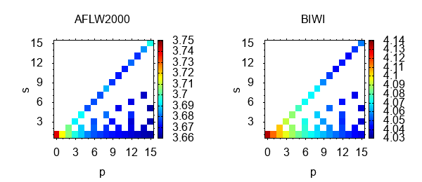
(a) Protocol 1

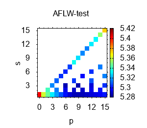
(b) Protocol 2

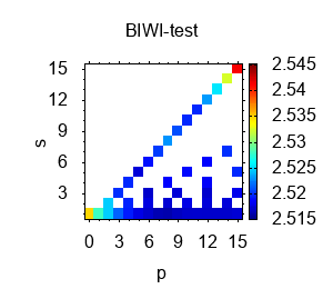
(c) Protocol 3

Figure 6: MAE heat map of results for various parameters of the convolutional ensemble: $p$ defines the size of the receptive field, $s$ defines the sparsity. Increasing $s$ decreases computations, and increasing $p$ increases computations. The figure contains white spots because $s$ must be a divisor of $p$.

The size of the ensemble depends quadratically on the value of $p$ and is inversely proportional to the square of $s$. Having a large ensemble can significantly reduce the performance. Therefore, it is necessary to consider the size of the ensemble when choosing the optimal values of $s$ and $p$.

5.3 Second stage

Based on the results of the first stage, the best parameters of the convolutional ensemble were determined. The maximum improvement is achieved on the first test protocol with $p=15$ and $s=5$. Other protocols have results comparable to the optimal one with these parameters.

In the second stage, various architectures of the ResNet family were used as the backbone: ResNet18, ResNet34, ResNet50, ResNet101 and ResNet152. All backbones were pre-trained on ImageNet. A single head branch was also used: a classification head with a bin size of 1.

The NN was trained using the Adam optimizer with a learning rate of $3\cdot 10^{-4}$ for 100 epochs. The batch size was 128.

Table V summarizes the results of the experiments for each test protocol and their comparison with the SOTA results. The best results in Table V are highlighted in bold.

Fig. 7 shows examples of predictions of a trained NN with ResNet152 backbone for all test protocols.

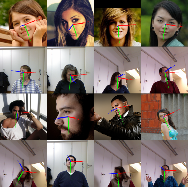
Figure 7: Visualization of ResNet152 predictions. The first two lines correspond to Test protocol 1, AFLW2000, and BIWI datasets, respectively. The second line corresponds to Test protocol 2, the AFLW dataset. The third line corresponds to Test protocol 3, the BIWI dataset. Bold lines correspond to the prediction, and thin lines correspond to the ground truth.

6 Discussion

This section discusses the results obtained for each test protocol and each element of the KD workflow.

6.1 Test protocol 1

In the first test protocol, the convolutional ensemble increases the quality of the prediction from $3.74$ to $3.67$ ($1.9\%$) for AFLW2000 and from $4.14$ to $4.04$ ($2.4\%$) for BIWI. The KD further improves the results. The improvement is achieved on all variants of the backbone. For AFLW2000, there is an improvement in the results with an increase in the depth of the backbone. The best result is achieved with the ResNet152 backbone. The KD increases the prediction quality compared to the non-ensemble version from $3.74$ to $3.48$ ($7.0\%$) for AFLW2000 and from $4.14$ to $3.70$ ($10.6\%$) for BIWI.

The best result shown is superior to the SOTA results for AFLW2000. In particular, the increase is $9.1\%$: $3.48$ versus $3.83$. The result comparable to the SOTA result is obtained for BIWI: $3.70$ versus $3.66$, respectively. The difference is $1.0\%$.

The result obtained on BIWI can be explained by the previous SOTA result obtained with the implicit use of additional data about facial landmarks. We conducted pure experiments according to the test protocol without using additional data. We also used the YOLOv5 detector, which normalizes the positions of the bounding boxes relative to the face in all datasets. Some publications do not clearly describe how the bounding boxes were obtained for the datasets. As we mentioned earlier, choosing the bounding boxes can significantly improve the result without changing the method [34, 35].

6.2 Test protocol 2

Different researchers use a different division of AFLW into training and testing parts for the second test protocol. It does not allow us to compare the results of different methods objectively.

The convolutional ensemble for this protocol increases the prediction quality from $5.40$ to $5.32$ ($1.5\%$). The KD allows one to increase the prediction quality compared to the non-ensemble variant from $5.40$ to $5.10$ ($5.6\%$). Also, note that KD improves the quality of the convolutional ensemble on all the backbone options considered.

6.3 Test protocol 3

The convolutional ensemble for the third protocol slightly increases the prediction quality from $2.54$ to $2.52$ ($0.8\%$). The KD decreases the prediction quality compared to ensemble and non-ensemble variants. The best result increases the SOTA result from $2.80$ to $2.52$ ($10\%$).

Note that BIWI has high representativeness in terms of head poses but low representativeness in terms of shooting conditions and people since it was obtained in the laboratory and contains only 20 people. Apparently, the low representativeness in terms of shooting conditions and people does not show the strengths of the convolutional ensemble and the KD.

TABLE V: Comparison of head pose estimations

Method	Use	Protocol 1								Protocol 2				Protocol 3
	extra	AFLW2000				BIWI
	data	pitch	yaw	roll	avg.	pitch	yaw	roll	avg.	pitch	yaw	roll	avg.	pitch	yaw	roll	avg.
HopeNet [23]		$6.55$	$6.47$	$5.43$	$6.15$	$6.60$	$4.81$	$3.26$	$4.89$	$5.89$	$6.26$	$3.82$	$5.32$	$3.39$	$3.29$	$3.00$	$3.23$
FSA-Net [18]		$6.08$	$4.50$	$4.64$	$5.07$	$4.96$	$4.27$	$2.76$	$4.00$					$4.29$	$2.89$	$3.60$	$3.60$
QuatNet [19]		$5.61$	$3.97$	$3.92$	$4.50$	$5.49$	$4.01$	$2.93$	$4.14$	$4.31$	$\bf{3.93}$	$2.59$	$3.61$
Hybrid [21]		$6.28$	$4.82$	$5.14$	$5.40$
BBox Margin [34]		$6.37$	$5.07$	$4.99$	$5.48$	$7.25$	$4.59$	$6.15$	$6.00$
CNN + Heatmaps [39]	✓									$4.43$	$5.22$	$2.53$	$4.06$
FDN [24]		$5.61$	$3.78$	$3.88$	$4.42$	$4.70$	$4.52$	$2.56$	$3.93$					$3.98$	$3.00$	$2.88$	$3.29$
MNN [50]	✓	$4.69$	$3.34$	$3.48$	$3.83$	$4.61$	$3.98$	$\bf{2.39}$	$\bf{3.66}$	$\bf{3.07}$	$4.16$	$\bf{2.43}$	$\bf{3.22}$
HPE-40 [47]		$6.18$	$4.87$	$4.80$	$5.28$	$5.18$	$4.57$	$3.12$	$4.29$
TriNet [20]		$5.77$	$4.20$	$4.04$	$4.67$	$4.76$	$\bf{3.05}$	$4.11$	$3.97$					$3.04$	$\bf{2.44}$	$2.93$	$2.80$
WSM-LgR [80]	✓													$4.56$	$2.47$	$\bf{2.13}$	$3.05$
Base ResNet18		$5.05$	$3.07$	$3.52$	$3.88$	$5.51$	$4.52$	$3.16$	$4.40$	$6.29$	$5.37$	$4.65$	$5.44$	$3.61$	$2.85$	$2.77$	$3.08$
Base ResNet34		$4.95$	$3.04$	$3.38$	$3.79$	$5.19$	$4.47$	$3.35$	$4.34$	$6.21$	$5.58$	$4.66$	$5.48$	$3.07$	$2.67$	$2.49$	$2.74$
Base ResNet50		$4.86$	$3.06$	$3.30$	$3.74$	$5.18$	$4.12$	$3.11$	$4.14$	$6.42$	$5.38$	$4.42$	$5.40$	$2.86$	$2.59$	$2.15$	$2.54$
Base ResNet101		$5.03$	$3.19$	$3.42$	$3.88$	$5.38$	$4.34$	$3.17$	$4.30$	$6.17$	$5.38$	$4.40$	$5.32$	$2.56$	$2.55$	$2.34$	$2.49$
Base ResNet152		$4.86$	$3.13$	$3.35$	$3.78$	$5.05$	$4.09$	$3.10$	$4.08$	$5.92$	$5.54$	$4.29$	$5.25$	$2.71$	$2.55$	$2.19$	$2.48$
Ensemble ResNet18		$4.94$	$3.00$	$3.40$	$3.78$	$5.48$	$4.40$	$3.09$	$4.32$	$6.25$	$5.32$	$4.49$	$5.35$	$3.62$	$2.85$	$2.76$	$3.08$
Ensemble ResNet34		$4.95$	$2.98$	$3.34$	$3.76$	$5.19$	$4.39$	$3.31$	$4.30$	$6.12$	$5.51$	$4.58$	$5.40$	$3.04$	$2.65$	$2.49$	$2.73$
Ensemble ResNet50		$4.82$	$2.96$	$3.22$	$3.67$	$5.23$	$3.89$	$3.01$	$4.04$	$6.34$	$5.29$	$4.32$	$5.32$	$2.85$	$2.56$	$2.16$	$2.52$
Ensemble ResNet101		$4.99$	$3.12$	$3.42$	$3.85$	$5.31$	$4.25$	$3.11$	$4.22$	$6.09$	$5.30$	$4.29$	$5.23$	$\bf{2.53}$	$2.54$	$2.31$	$\bf{2.46}$
Ensemble ResNet152		$4.85$	$3.06$	$3.32$	$3.74$	$5.01$	$3.98$	$3.05$	$4.01$	$5.77$	$5.44$	$4.21$	$5.14$	$2.70$	$2.56$	$2.17$	$2.48$
KD-ResNet18		$4.69$	$3.00$	$3.22$	$3.64$	$5.07$	$3.96$	$3.06$	$4.03$	$6.02$	$5.45$	$4.16$	$5.21$	$2.82$	$2.59$	$2.34$	$2.58$
KD-ResNet34		$4.74$	$3.00$	$3.21$	$3.65$	$\bf{4.49}$	$4.06$	$2.96$	$3.83$	$6.10$	$5.39$	$4.24$	$5.24$	$2.93$	$2.59$	$2.35$	$2.62$
KD-ResNet50		$4.68$	$\bf{2.92}$	$3.11$	$3.57$	$4.80$	$4.05$	$2.94$	$3.93$	$6.04$	$5.38$	$4.28$	$5.24$	$2.87$	$2.73$	$2.34$	$2.65$
KD-ResNet101		$4.65$	$2.96$	$3.02$	$3.54$	$5.31$	$3.76$	$2.76$	$3.94$	$5.96$	$5.36$	$3.98$	$5.10$	$2.76$	$2.74$	$2.25$	$2.58$
KD-ResNet152		$\bf{4.52}$	$2.97$	$\bf{2.96}$	$\bf{3.48}$	$4.73$	$3.50$	$2.87$	$3.70$	$5.93$	$5.41$	$4.07$	$5.14$	$2.88$	$2.61$	$2.37$	$2.62$

6.4 Neural network and data preprocessing

Data preprocessing is an important part of NN training. Earlier, we demonstrated [25] that using rotation augmentation and a NN with one RvC head allows us to get a result that is slightly inferior only to MNN. In particular, MAE is equal to 3.85 in the first test protocol on AFLW2000. MAE is equal to 4.95 without rotation augmentation, which is better than many previous works [23, 18, 21, 47]. This accuracy is increased by bounding boxes relabeling obtained by the YOLOv5 detector.

In this paper, we have added additional augmentations and improved the NN architecture. Additional augmentations manipulate the color scheme and add noise. We have added additional heads, which provide regularization during the NN training. At the same time, removing any head branch increased the error. The improvements have reduced MAE for ResNet50 to 3.74 on AFLW2000. It is better than any previous job with the same backbone.

Base ResNet50 results worse than some works [18, 24, 50, 20] on BIWI in the 1st test protocol. It is due to the low representativeness of 300W-LP relative to BIWI. In the 3rd test protocol, based on BIWI, the proposed architecture achieves better results than all the previous ones. The proposed angle coding scheme is less resistant to outliers but is better suited for KD.

6.5 Convolutional ensemble

The proposed ensemble increases prediction accuracy using a single trained NN. A wide alternative NN operating with an enlarged image does not improve the result. As described in section 3.3, the NN does not receive critical information about the image borders by padding function. In a sense, the convolutional ensemble is a kind of test time augmentation.

The convolutional ensemble increases accuracy on all test protocols by smoothing off outliers. The ensemble has the most significant increase in the 1st test protocol with the largest training dataset. The ensemble based on ResNet50 has the best quality. The ensemble design reduces the dependence on the image boundaries and, consequently, the face bounding box. However, independent prediction for each offset significantly increases computational costs by 49 times.

6.6 Knowledge distillation

Initially, we decided to use KD to compress the ensemble into a single NN. The most suitable method of KD from the ensemble is the response-based method. Other KD methods from the ensemble are laborious without a guaranteed result. The naive response-based method for the regression problem is inefficient. Therefore, we use the RvC head, which reduces the regression problem to the classification problem. The student trained by the response-based method always has worse results than the teacher for the classification problem [30, 31, 32, 33]. We expected that KD would compensate for the ensemble gain. However, we unexpectedly received a boost of convolutional ensemble predictions.

We use a convolutional ensemble based on ResNet50 as a teacher in all test protocols. There is the KD boosting effect on the 1st and 2nd test protocols. However, we can correctly compare the 1st test protocol with previous works. KD-ResNet18 is inferior to previous works only on BIWI. At the same time, KD-ResNet18 requires significantly fewer computing resources. KD-ResNet50 is inferior to [50] only on BIWI but overtakes all previous work on AFLW2000. Also, KD allows one to train deeper NN models with increased accuracy. Base ResNet152 slightly improves the results of Base ResNet50 on BIWI but worsens the results on AFLW2000. KD-ResNet152 demonstrates a significant increase in accuracy on both datasets.

Proposed NN architecture, convolutional ensemble, and KD based on RvC improve the HPE accuracy. The proposed method can be used not only to compress NNs but also as a training method to obtain NNs with maximum accuracy. Perhaps the proposed method will be effective for other regression problems as well.

7 Conclusion

We propose a data preprocessing method and a NN architecture containing four RvC heads and one regression head. These innovations improve the results of previous work in some test protocols. ResNet50 trained on 300W-LP reduces MAE to 3.74 on AFLW2000.

We propose the convolutional ensemble that reduces outliers and dependence on image boundaries. The convolutional ensemble is a kind of test time augmentation. The ensemble improves the quality of the base NN on all test protocols.

We propose the response-based method of KD for the HPE problem. A student trained by the response-based method always has results worse than the teacher model for the classification problem [30, 31, 32, 33]. For naive regression, the response-based method is useless. A student trained by the proposed method achieves results better than a teacher. This unexpected feature makes it possible to use KD as a booster. The proposed method provides an increased accuracy due to a deeper ResNet152, which without KD has an accuracy near ResNet50. KD improves the results by an average of 7.7% compared to the non-ensemble version. The results obtained either significantly exceed or are comparable with the SOTA results.

We have made the trained NNs publicly available [73]. ResNet152 obtains the best results in terms of accuracy. ResNet18 obtains a better result on AFLW2000 than any previous method. ResNet18 may be of interest for application tasks where maximum performance is important.

We have made publicly available the face bounding boxes [73] for 300W-LP, AFLW, AFLW2000, and BIWI. This labeling allows one to perform a more objective comparison of methods and level out the errors associated with the choice of the bounding boxes.

Andrey Sheka A. S. Sheka is a researcher in the Laboratory of Complex Systems Analysis of the Computational Systems Department at the N.N. Krasovskii Institute of Mathematics and Mechanics. His main research interests are Deep Learning, Computer Vision and Behavioral Analysis. He has published over 30 publications on data analysis, artificial intelligence, and computational optimization.

Victor Samun V. S. Samun is a researcher in the Laboratory of Complex Systems Analysis of the Computational Systems Department at the N.N. Krasovskii Institute of Mathematics and Mechanics. His main research interests are Deep Learning and Computer Vision. He has published 5 publications on high-performance computing, machine learning, and artificial intelligence.

References

- Osadchy et al. [2007] M. Osadchy, Y. Le Cun, and M. L. Miller, “Synergistic face detection and pose estimation with energy-based models,” Journal of Machine Learning Research, vol. 8, 2007.
- Wu and Ji [2019] Y. Wu and Q. Ji, “Facial Landmark Detection: A Literature Survey,” International Journal of Computer Vision, vol. 127, no. 2, 2019.
- Chen et al. [2017] S. Chen, C. Zhang, M. Dong, J. Le, and M. Rao, “Using ranking-CNN for age estimation,” in Proceedings - 30th IEEE Conference on Computer Vision and Pattern Recognition, CVPR 2017, vol. 2017-January, 2017.
- Murphy-Chutorian and Trivedi [2009] E. Murphy-Chutorian and M. M. Trivedi, “Head pose estimation in computer vision: A survey,” IEEE Transactions on Pattern Analysis and Machine Intelligence, vol. 31, no. 4, 2009.
- Cao et al. [2018] K. Cao, Y. Rong, C. Li, X. Tang, and C. C. Loy, “Pose-Robust Face Recognition via Deep Residual Equivariant Mapping,” in Proceedings of the IEEE Computer Society Conference on Computer Vision and Pattern Recognition, 2018.
- Zhang et al. [2018a] F. Zhang, T. Zhang, Q. Mao, and C. Xu, “Joint Pose and Expression Modeling for Facial Expression Recognition,” in Proceedings of the IEEE Computer Society Conference on Computer Vision and Pattern Recognition, 2018.
- Langton et al. [2004] S. R. Langton, H. Honeyman, and E. Tessler, “The influence of head contour and nose angle on the perception of eye-gaze direction,” Perception and Psychophysics, vol. 66, no. 5, 2004.
- Liu et al. [2008] K. Liu, Y. P. Luo, G. Tei, and S. Y. Yang, “Attention recognition of drivers based on head pose estimation,” in 2008 IEEE Vehicle Power and Propulsion Conference, VPPC 2008, 2008.
- Passalis and Tefas [2020] N. Passalis and A. Tefas, “Continuous drone control using deep reinforcement learning for frontal view person shooting,” Neural Computing and Applications, vol. 32, no. 9, 2020.
- Huang et al. [2002] J. Huang, X. Shao, and H. Wechsler, “Face pose discrimination using support vector machines (SVM),” 2002.
- Tzimiropoulos and Pantic [2017] G. Tzimiropoulos and M. Pantic, “Fast Algorithms for Fitting Active Appearance Models to Unconstrained Images,” International Journal of Computer Vision, vol. 122, no. 1, 2017.
- Balasubramanian et al. [2007] V. N. Balasubramanian, J. Ye, and S. Panchanathan, “Biased manifold embedding: A framework for person-independent head pose estimation,” in Proceedings of the IEEE Computer Society Conference on Computer Vision and Pattern Recognition, 2007.
- Zhu et al. [2016] X. Zhu, Z. Lei, X. Liu, H. Shi, and S. Z. Li, “Face alignment across large poses: A 3D solution,” in Proceedings of the IEEE Computer Society Conference on Computer Vision and Pattern Recognition, vol. 2016-December, 2016.
- Kumar et al. [2018] A. Kumar, A. Alavi, and R. Chellappa, “KEPLER: Simultaneous estimation of keypoints and 3D pose of unconstrained faces in a unified framework by learning efficient H-CNN regressors,” Image and Vision Computing, vol. 79, 2018.
- Hu et al. [2004] Y. Hu, L. Chen, Y. Zhou, and H. Zhang, “Estimating face pose by facial asymmetry and geometry,” in Proceedings - Sixth IEEE International Conference on Automatic Face and Gesture Recognition, 2004.
- Huang et al. [2010] C. Huang, X. Ding, and C. Fang, “Head pose estimation based on random forests for multiclass classification,” in Proceedings - International Conference on Pattern Recognition, 2010.
- Shao et al. [2020] X. Shao, Z. Qiang, H. Lin, Y. Dong, and X. Wang, “A survey of head pose estimation methods,” in 2020 International Conferences on Internet of Things (iThings), Nov 2020, pp. 787–796.
- Yang et al. [2019] T. Y. Yang, Y. T. Chen, Y. Y. Lin, and Y. Y. Chuang, “FSA-Net: Learning fine-grained structure aggregation for head pose estimation from a single image,” in Proceedings of the IEEE Computer Society Conference on Computer Vision and Pattern Recognition, vol. 2019-June, 2019.
- Hsu et al. [2019] H. W. Hsu, T. Y. Wu, S. Wan, W. H. Wong, and C. Y. Lee, “Quatnet: Quaternion-based head pose estimation with multiregression loss,” IEEE Transactions on Multimedia, vol. 21, no. 4, 2019.
- Cao et al. [2020] Z. Cao, Z. Chu, D. Liu, and Y. Chen, “A vector-based representation to enhance head pose estimation,” 2020.
- Wang et al. [2019a] Y. Wang, W. Liang, J. Shen, Y. Jia, and L. F. Yu, “A deep Coarse-to-Fine network for head pose estimation from synthetic data,” Pattern Recognition, vol. 94, 2019.
- Wang et al. [2019b] H. Wang, Z. Chen, and Y. Zhou, “Hybrid coarse-fine classification for head pose estimation,” 2019.
- Ruiz et al. [2018] N. Ruiz, E. Chong, and J. M. Rehg, “Fine-grained head pose estimation without keypoints,” in IEEE Computer Society Conference on Computer Vision and Pattern Recognition Workshops, vol. 2018-June, 2018.
- Zhang et al. [2020] H. Zhang, M. Wang, Y. Liu, and Y. Yuan, “FDN: Feature Decoupling Network for Head Pose Estimation,” Proceedings of the AAAI Conference on Artificial Intelligence, vol. 34, no. 07, 2020.
- Sheka and Samun [2021a] A. Sheka and V. Samun, “Rotation augmentation for head pose estimation problem,” in 2021 Ural Symposium on Biomedical Engineering, Radioelectronics and Information Technology (USBEREIT), 2021, pp. 0308–0311.
- Sharkey [1996] A. J. Sharkey, “On Combining Artificial Neural Nets,” Connection Science, vol. 8, no. 3-4, 1996.
- Yang et al. [2013] J. Yang, X. Zeng, S. Zhong, and S. Wu, “Effective neural network ensemble approach for improving generalization performance,” IEEE Transactions on Neural Networks and Learning Systems, vol. 24, no. 6, 2013.
- Liang et al. [2014] H. Liang, L. Burgio, K. Bailey, A. Lucian, C. Dilley, S. Bellesia, C. Cheung, and C. Brooks, “Distilling the knowledge in a neural network (Godfather’s Work),” Studies in Conservation, vol. 59, no. sup1, 2014.
- Yim et al. [2017] J. Yim, D. Joo, J. Bae, and J. Kim, “A gift from knowledge distillation: Fast optimization, network minimization and transfer learning,” in Proceedings - 30th IEEE Conference on Computer Vision and Pattern Recognition, CVPR 2017, vol. 2017-January, 2017.
- Gou et al. [2020] J. Gou, B. Yu, S. J. Maybank, and D. Tao, “Knowledge Distillation: A Survey,” 2020.
- Bucilua et al. [2006] C. Bucilua, R. Caruana, and A. Niculescu-Mizil, “Model compression,” in Proceedings of the 12th ACM SIGKDD International Conference on Knowledge Discovery and Data Mining, ser. KDD ’06. New York, NY, USA: Association for Computing Machinery, 2006, p. 535–541.
- Ba and Caruana [2014] J. Ba and R. Caruana, “Do deep nets really need to be deep?” in Advances in Neural Information Processing Systems, Z. Ghahramani, M. Welling, C. Cortes, N. Lawrence, and K. Q. Weinberger, Eds., vol. 27. Curran Associates, Inc., 2014.
- Hinton et al. [2015] G. Hinton, O. Vinyals, and J. Dean, “Distilling the knowledge in a neural network,” 2015.
- Shao et al. [2019] M. Shao, Z. Sun, M. Ozay, and T. Okatani, “Improving head pose estimation with a combined loss and bounding box margin adjustment,” 2019.
- Xue et al. [2020] A. Xue, K. Sheng, S. Dai, and X. Li, “Robust landmark-free head pose estimation by learning to crop and background augmentation,” IET Image Processing, vol. 14, no. 11, 2020.
- Gao et al. [2003] X. S. Gao, X. R. Hou, J. Tang, and H. F. Cheng, “Complete solution classification for the perspective-three-point problem,” IEEE Transactions on Pattern Analysis and Machine Intelligence, vol. 25, no. 8, 2003.
- Li et al. [2012] S. Li, C. Xu, and M. Xie, “A robust O(n) solution to the perspective-n-point problem,” IEEE Transactions on Pattern Analysis and Machine Intelligence, vol. 34, no. 7, 2012.
- Liu et al. [2021] L. Liu, Z. Ke, J. Huo, and J. Chen, “Head pose estimation through keypoints matching between reconstructed 3d face model and 2d image,” Sensors, vol. 21, no. 5, 2021.
- Gupta et al. [2019] A. Gupta, K. Thakkar, V. Gandhi, and P. J. Narayanan, “Nose, Eyes and Ears: Head Pose Estimation by Locating Facial Keypoints,” in ICASSP, IEEE International Conference on Acoustics, Speech and Signal Processing - Proceedings, vol. 2019-May, 2019.
- Fischler and Bolles [1981] M. A. Fischler and R. C. Bolles, “Random sample consensus: A Paradigm for Model Fitting with Applications to Image Analysis and Automated Cartography,” Communications of the ACM, vol. 24, no. 6, 1981.
- Sheka and Samun [2020] A. S. Sheka and V. S. Samun, “Determining the angles of head rotation on a selective set of facial keypoints,” in AIP Conference Proceedings, vol. 2313, 2020.
- Yuan et al. [2020] H. Yuan, M. Li, J. Hou, and J. Xiao, “Single image-based head pose estimation with spherical parametrization and 3D morphing,” Pattern Recognition, vol. 103, 2020.
- Ranjan et al. [2016] R. Ranjan, V. M. Patel, and R. Chellappa, “HyperFace: A Deep Multi-task Learning Framework for Face Detection, Landmark Localization, Pose Estimation, and Gender Recognition,” IEEE Transactions on Pattern Analysis and Machine Intelligence, 2016.
- Chang et al. [2017] F. J. Chang, A. T. Tran, T. Hassner, I. Masi, R. Nevatia, and G. Medioni, “FacePoseNet: Making a Case for Landmark-Free Face Alignment,” in Proceedings - 2017 IEEE International Conference on Computer Vision Workshops, ICCVW 2017, vol. 2018-January, 2017.
- Gu et al. [2017] J. Gu, X. Yang, S. De Mello, and J. Kautz, “Dynamic facial analysis: From Bayesian filtering to recurrent neural network,” in Proceedings - 30th IEEE Conference on Computer Vision and Pattern Recognition, CVPR 2017, vol. 2017-January, 2017.
- Torgo and Gama [1996] L. Torgo and J. Gama, “Regression by classification,” in Lecture Notes in Computer Science, 1996.
- Huang et al. [2020] B. Huang, R. Chen, W. Xu, and Q. Zhou, “Improving head pose estimation using two-stage ensembles with top-k regression,” Image and Vision Computing, vol. 93, 2020.
- Venturelli et al. [2017] M. Venturelli, G. Borghi, R. Vezzani, and R. Cucchiara, “From depth data to head pose estimation: A Siamese approach,” in VISIGRAPP 2017 - Proceedings of the 12th International Joint Conference on Computer Vision, Imaging and Computer Graphics Theory and Applications, vol. 5, 2017.
- Borghi et al. [2020] G. Borghi, M. Fabbri, R. Vezzani, S. Calderara, and R. Cucchiara, “Face-from-Depth for Head Pose Estimation on Depth Images,” IEEE Transactions on Pattern Analysis and Machine Intelligence, vol. 42, no. 3, 2020.
- Valle et al. [2020] R. Valle, J. M. Buenaposada, and L. Baumela, “Multi-task head pose estimation in-the-wild,” IEEE Transactions on Pattern Analysis and Machine Intelligence, 2020.
- Zhang et al. [2018b] J. Zhang, T. Liu, and D. Tao, “An information-theoretic view for deep learning,” 2018.
- Allen-Zhu et al. [2019] Z. Allen-Zhu, Y. Li, and Y. Liang, Learning and Generalization in Overparameterized Neural Networks, Going beyond Two Layers. Red Hook, NY, USA: Curran Associates Inc., 2019.
- Wu et al. [2016] J. Wu, C. Leng, Y. Wang, Q. Hu, and J. Cheng, “Quantized convolutional neural networks for mobile devices,” in 2016 IEEE Conference on Computer Vision and Pattern Recognition (CVPR). Los Alamitos, CA, USA: IEEE Computer Society, jun 2016, pp. 4820–4828.
- Reed [1993] R. Reed, “Pruning algorithms-a survey,” IEEE Transactions on Neural Networks, vol. 4, no. 5, pp. 740–747, 1993.
- Park and Kwak [2019] S. Park and N. Kwak, “Feed: Feature-level ensemble for knowledge distillation,” 2019.
- Kim et al. [2020] J. Kim, S. Park, and N. Kwak, “Paraphrasing complex network: Network compression via factor transfer,” 2020.
- Li et al. [2020] G. Li, J. Zhang, Y. Wang, C. Liu, M. Tan, Y. Lin, W. Zhang, J. Feng, and T. Zhang, “Residual distillation: Towards portable deep neural networks without shortcuts,” in Advances in Neural Information Processing Systems, H. Larochelle, M. Ranzato, R. Hadsell, M. F. Balcan, and H. Lin, Eds., vol. 33. Curran Associates, Inc., 2020, pp. 8935–8946.
- He et al. [2016] K. He, X. Zhang, S. Ren, and J. Sun, “ResNet,” Proceedings of the IEEE Computer Society Conference on Computer Vision and Pattern Recognition, 2016.
- Dietterich [2000] T. G. Dietterich, “Ensemble methods in machine learning,” in Lecture Notes in Computer Science, vol. 1857 LNCS, 2000.
- Asif et al. [2020] U. Asif, J. Tang, and S. Harrer, “Ensemble knowledge distillation for learning improved and efficient networks,” in Frontiers in Artificial Intelligence and Applications, vol. 325, 2020.
- Kullback and Leibler [1951] S. Kullback and R. A. Leibler, “On Information and Sufficiency,” The Annals of Mathematical Statistics, vol. 22, no. 1, 1951.
- Köstinger et al. [2011] M. Köstinger, P. Wohlhart, P. M. Roth, and H. Bischof, “Annotated facial landmarks in the wild: A large-scale, real-world database for facial landmark localization,” in Proceedings of the IEEE International Conference on Computer Vision, 2011.
- Fanelli et al. [2013] G. Fanelli, M. Dantone, J. Gall, A. Fossati, and L. Van Gool, “Random Forests for Real Time 3D Face Analysis,” International Journal of Computer Vision, vol. 101, no. 3, 2013.
- Zhu and Ramanan [2012] X. Zhu and D. Ramanan, “Face detection, pose estimation, and landmark localization in the wild,” in Proceedings of the IEEE Computer Society Conference on Computer Vision and Pattern Recognition, 2012.
- Belhumeur et al. [2013] P. N. Belhumeur, D. W. Jacobs, D. J. Kriegman, and N. Kumar, “Localizing parts of faces using a consensus of exemplars,” IEEE Transactions on Pattern Analysis and Machine Intelligence, 2013.
- Zhou et al. [2013] E. Zhou, H. Fan, Z. Cao, Y. Jiang, and Q. Yin, “Extensive facial landmark localization with coarse-to-fine convolutional network cascade,” in Proceedings of the IEEE International Conference on Computer Vision, 2013.
- Sagonas et al. [2013] C. Sagonas, G. Tzimiropoulos, S. Zafeiriou, and M. Pantic, “300 faces in-the-wild challenge: The first facial landmark Localization Challenge,” in Proceedings of the IEEE International Conference on Computer Vision, 2013.
- Ren et al. [2017] S. Ren, K. He, R. Girshick, and J. Sun, “Faster R-CNN: Towards Real-Time Object Detection with Region Proposal Networks,” IEEE Transactions on Pattern Analysis and Machine Intelligence, vol. 39, no. 6, 2017.
- Zhang et al. [2016] K. Zhang, Z. Zhang, Z. Li, and Y. Qiao, “Joint Face Detection and Alignment Using Multitask Cascaded Convolutional Networks,” IEEE Signal Processing Letters, vol. 23, no. 10, 2016.
- King [2009] D. E. King, “Dlib-ml: A machine learning toolkit,” Journal of Machine Learning Research, vol. 10, 2009.
- yol [2021] “YOLO V5 detector,” 2021. [Online]. Available: https://github.com/ultralytics/yolov5
- Yang et al. [2016] S. Yang, P. Luo, C. C. Loy, and X. Tang, “WIDER FACE: A face detection benchmark,” in Proceedings of the IEEE Computer Society Conference on Computer Vision and Pattern Recognition, vol. 2016-December, 2016.
- Sheka and Samun [2021b] A. Sheka and V. Samun, “Head pose estimation models and dataset labeling,” 2021. [Online]. Available: https://github.com/AndreySheka/kd_oe_hpe
- Wang and Perez [2017] J. Wang and L. Perez, “The effectiveness of data augmentation in image classification using deep learning,” 2017.
- Mikołajczyk and Grochowski [2018] A. Mikołajczyk and M. Grochowski, “Data augmentation for improving deep learning in image classification problem,” in 2018 International Interdisciplinary PhD Workshop, IIPhDW 2018, 2018.
- Buslaev et al. [2020] A. Buslaev, V. I. Iglovikov, E. Khvedchenya, A. Parinov, M. Druzhinin, and A. A. Kalinin, “Albumentations: Fast and flexible image augmentations,” Information (Switzerland), vol. 11, no. 2, 2020.
- Amador et al. [2018] E. Amador, R. Valle, J. M. Buenaposada, and L. Baumela, “Benchmarking head pose estimation in-the-wild,” in Lecture Notes in Computer Science, vol. 10657 LNCS, 2018.
- Jia Deng et al. [2009] Jia Deng, Wei Dong, R. Socher, Li-Jia Li, Kai Li, and Li Fei-Fei, “ImageNet: A large-scale hierarchical image database,” 2009.
- Kingma and Ba [2015] D. P. Kingma and J. L. Ba, “Adam: A method for stochastic optimization,” in 3rd International Conference on Learning Representations, ICLR 2015 - Conference Track Proceedings, 2015.
- Abate et al. [2020] A. F. Abate, P. Barra, C. Pero, and M. Tucci, “Head pose estimation by regression algorithm,” Pattern Recognition Letters, vol. 140, 2020.