DL-Traff: Survey and Benchmark of Deep Learning Models for Urban Traffic Prediction

Abstract.

Nowadays, with the rapid development of IoT (Internet of Things) and CPS (Cyber-Physical Systems) technologies, big spatiotemporal data are being generated from mobile phones, car navigation systems, and traffic sensors. By leveraging state-of-the-art deep learning technologies on such data, urban traffic prediction has drawn a lot of attention in AI and Intelligent Transportation System community. The problem can be uniformly modeled with a 3D tensor (T, N, C), where T denotes the total time steps, N denotes the size of the spatial domain (i.e., mesh-grids or graph-nodes), and C denotes the channels of information. According to the specific modeling strategy, the state-of-the-art deep learning models can be divided into three categories: grid-based, graph-based, and multivariate time-series models. In this study, we first synthetically review the deep traffic models as well as the widely used datasets, then build a standard benchmark to comprehensively evaluate their performances with the same settings and metrics. Our study named DL-Traff is implemented with two most popular deep learning frameworks, i.e., TensorFlow and PyTorch, which is already publicly available as two GitHub repositories https://github.com/deepkashiwa20/DL-Traff-Grid and https://github.com/deepkashiwa20/DL-Traff-Graph. With DL-Traff, we hope to deliver a useful resource to researchers who are interested in spatiotemporal data analysis.

Grid-Based	Venue	Cite	Dataset (* means Open)	Prediction Task	Metric
ST-ResNet(Zhang et al., 2017)	AAAI17	867	TaxiBJ*, BikeNYC*	Taxi In-Out Flow	RMSE
DeepSD(Wang et al., 2017)	ICDE17	125	Didi Taxi (HangZhou)	Taxi Demand	MAE, RMSE
DMVST-Net(Yao et al., 2018)	AAAI18	456	Didi Taxi (GuangZhou)	Taxi Demand	RMSE, MAPE
Periodic-CRN(Zonoozi et al., 2018)	IJCAI18	57	TaxiBJ*, TaxiSG	Taxi Density/In-Out Flow	RMSE
Hetero-ConvLSTM(Yuan et al., 2018)	KDD18	121	Vehicle Crash Data*	Traffic Accident	MSE, RMSE, CE
DeepSTN+(Lin et al., 2019)	AAAI19	53	MobileBJ, BikeNYC-I*	Crowd/Taxi In-Out Flow	MAE, RMSE
STDN(Yao et al., 2019)	AAAI19	204	TaxiNYC*, BikeNYC-II*	Taxi/Bike O-D Number	RMSE, MAPE
MDL(Zhang et al., 2019)	TKDE19	92	TaxiBJ, BikeNYC	Taxi Transition/In-Out Flow	MAE, RMSE
DeepUrbanEvent(Jiang et al., 2019)	KDD19	32	Konzatsu Toukei	Crowd Density/Flow	MSE
Curb-GAN (Zhang et al., 2020b)	KDD20	1	Taxi Speed/Inflow (Shenzhen)*	Taxi Speed/Inflow	RMSE, MAPE
Graph-Based	Venue	Cite	Dataset (* means Open)	Prediction Task	Metric
STGCN(Yu et al., 2018)	IJCAI18	660	BJER4, PeMSD7(M)*, PeMSD7(L)	Traffic Volume/Speed	MAE, RMSE, MAPE
DCRNN(GCGRU)(Li et al., 2018)	ICLR18	691	METR-LA*, PeMS-BAY*	Traffic Volume/Speed	MAE, RMSE, MAPE
Multi-graph(Chai et al., 2018)	SIGSPATIAL18	89	Bike Flow (New York and Chicago)	Bike In-Out Flow	RMSE
ASTGCN(Guo et al., 2019)	AAAI19	239	PeMSD4-I*, PeMSD8-I*	Traffic Volume/Speed	MAE, RMSE
DGCNN(Diao et al., 2019)	AAAI19	56	TrafficNYC, PeMS	Traffic Volume/Speed	MAE, RMSE
ST-MGCN(Geng et al., 2019)	AAAI19	182	Bike Demand (Beijing and Shanghai)	Bike Demand	MAE, RMSE, MAPE
Graph WaveNet(Wu et al., 2019)	IJCAI19	144	METR-LA*, PeMS-BAY*	Traffic Volume/Speed	MAE, RMSE, MAPE
STG2Seq(Bai et al., 2019)	IJCAI19	33	DidiSY, BikeNYC*, TaxiBJ*	Taxi/Bike Demand	MAE, RMSE, MAPE
T-GCN(Zhao et al., 2019)	TITS19	195	TaxiSZ*, METR-LA*	Traffic Volume/Speed	MAE, RMSE, Acc, $R^{2}$, var
TGC-LSTM(Cui et al., 2019)	TITS19	166	Seattle-Loop*, INRIX Traffic	Traffic Volume/Speed	MAE, RMSE, MAPE
GCGA(Yu and Gu, 2019)	TITS19	27	Cologne Traffic	Traffic Volume/Speed	MAPE
GMAN(Zheng et al., 2020)	AAAI20	73	Taxi Xiamen, PeMS-BAY*	Traffic Volume/Speed	MAE, RMSE, MAPE
MRA-BGCN(Chen et al., 2020)	AAAI20	28	METR-LA*, PeMS-BAY*	Traffic Volume/Speed	MAE, RMSE, MAPE
STSGCN(Song et al., 2020)	AAAI20	39	PeMS03*, PeMS04*, PeMS07*, PeMS08*	Traffic Volume/Speed	MAE, RMSE, MAPE
SLCNN(Zhang et al., 2020a)	AAAI20	13	METR-LA*, PeMS-BAY*,	Traffic Volume/Speed	MAE, RMSE, MAPE
			PeMSD7(M)*, BJF, BRF, BRF-L
STGNN(Wang et al., 2020)	WWW20	24	METR-LA*, PeMS-BAY*	Traffic Volume/Speed	MAE, RMSE, MAPE
H-STGCN(Dai et al., 2020)	KDD20	9	W3-715, E5-2907 (Beijing)	Traffic Volume/Speed	MAE, MAPE, RMSE
AGCRN(Bai et al., 2020)	NeurIPS20	9	PeMSD4*, PeMSD8*	Traffic Volume/Speed	MAE, RMSE, MAPE
T-MGCN(Lv et al., 2020)	TITS20	7	HZJTD*, PeMSD10*	Traffic Volume/Speed	MAE, RMSE, MAPE
DGCN(Guo et al., 2020)	TITS20	1	PeMSD4*, PeMSD8*, PHILADELPHIA	Traffic Volume/Speed	MAE, RMSE
Multivariate Time-Series	Venue	Cite	Dataset (* means Open)	Prediction Task	Metric
LSTNet(Lai et al., 2018)	SIGIR18	318	PeMS-BAY*, Solar-Energy*	Multivariate Time-Series	RSE, CORR
			Electricity*, Exchange Rate*	Traffic Volume/Speed
GaAN(GGRU)(Zhang et al., 2018)	UAI18	214	PPI, Reddit, METR-LA*	Node Classification	MAE, RMSE
				Traffic Volume/Speed
GeoMAN(Liang et al., 2018)	IJCAI18	182	Water Quality, Air Quality	Multivariate Time-Series	MAE, RMSE
ST-MetaNet(Pan et al., 2019)	KDD19	91	TaxiBJ-I*, METR-LA*	Taxi In-Out Flow	MAE, RMSE
				Traffic Volume/Speed
TPA-LSTM (Shih et al., 2019)	ECMLPKDD19	88	Solar Energy*, Traffic(PeMS)*, ,	Multivariate Time-Series	RAE, RSE, CORR
			Electricity*, Music*, Exchange Rate*	Traffic Volume/Speed
Transformer(Li et al., 2019)	NeurIPS19	84	Electricity*, Traffic*, Solar*, Wind*	Multivariate Time-Series	$\rho$-quantile
MTGNN(Wu et al., 2020)	KDD20	32	Solar-Energy*, Taffic(PeMS)*	Multivariate Time-Series	MAE, RMSE, MAPE
			Electricity*, Exchange-Rate*	Traffic Volume/Speed	RSE, CORR

Table 1. Summary of The State-Of-The-Art Models *Citation number was referred from Google Scholar by 2021/6/13*

1. Introduction

Nowadays, with the rapid development of IoT (Internet of Things) and CPS (Cyber-Physical Systems) technologies, big spatiotemporal data are being generated from mobile phones, car navigation systems, and traffic sensors. Based on such data, urban traffic prediction has been taken as a significant research problem and a key technique for building smart city, especially intelligent transportation system. From 2014 to 2017, encouraged by the huge success of deep learning technologies in the Computer Vision and Natural Language Processing field, researchers in the Intelligent Transportation System community, started to apply Long-Term Short Memory (LSTM) and Convolution Neural Network (CNN) to the well-established traffic prediction task(Huang et al., 2014; Lv et al., 2014; Ma et al., 2015, 2017), and also achieved an unprecedented success. Following these pioneers, researchers have leveraged the state-of-the-art deep learning technologies to develop various prediction models and publish a big amount of studies on the major AI and transportation venues as listed in Table 1. Although the prediction tasks may slightly differ from each other, they can all be categorized as deep traffic models.

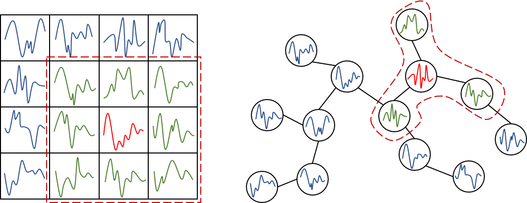
Figure 1. Grid-Based Traffic and Graph-Based Traffic.

No matter based on grid or graph, the traffic data illustrated in Fig.1 can be uniformly represented with a 3D tensor $\mathbb{R}^{T\times N\times C}$, where T denotes the size of the temporal domain (i.e., timeslots with constant sampling rate), N denotes the size of the spatial domain (i.e., mesh-grids or graph-nodes), and C denotes the number of information channels. For instance, assuming 300 traffic sensors are deployed to record traffic speed (channel1) and volume (channel2) every 30 minutes for 100 consecutive days, then the total data can be represented by tensor $\mathbb{R}^{4800\times 300\times 2}$. Besides traffic volume and speed, channels can also be used to store crowd density, taxi demand, traffic accident, car/ride-hailing order, and crowd/taxi/bike inflow and outflow. More specifically, grid-based model meshes the entire spatial domain into $H\times W$ fine-grained mesh-grids and converts the 3D representation into 4D tensor $\mathbb{R}^{T\times H\times W\times C}$ format. Graph-based model introduces directed or undirected graph $G$ = $(V,E)$ to utilize the topological structure of the urban road network for modeling, where $v\in V$ is a node, $|V|$ = $N$, and $e\in E$ is an edge. Multivariate time-series model naturally takes the N spatial units as N time-series variates and shares the same representation, i.e., $\mathbb{R}^{T\times N\times C}$ with graph-based model. Thus, the deep learning models listed in Table 1 can be divided into three groups according to the specific modeling strategy along the spatial axis.

Through the citation number in Table 1, we can know how much attention these studies have drawn in our AI and data science community. But due to the huge amount of the related works, researchers are often too exhausted to follow up with the specific details of each model. More importantly, the evaluations on this family of models are still confusing and not well organized. For instance, some models demonstrated superior performances to the existing ones by using different datasets or metrics as shown in Table 1, while some models utilized a self-designed objective function or employed extra data sources such as Point-of-Interest (POI) data (Lin et al., 2019) or navigation app data (Dai et al., 2020) to achieve better prediction accuracy. To address the problems above, a concise but precise survey will be a great help for researchers involved in this emerging topic. But only a survey is not enough. It is also significant to conduct standard performance evaluations to examine the true function of each spatial and temporal component by using the same datasets, metrics, and other experimental settings. This paper fills these needs by providing a concise survey followed by a comprehensive benchmark evaluation on the recent deep traffic models.

We first define two benchmark tasks in Section 2, one is single-step prediction for inflow and outflow based on grid-based traffic data, another is multi-step prediction for traffic speed based on graph-based data. Second, in Section 3, we investigate both of the grid-based and graph-based datasets and pick up some open and widely used ones as our benchmark data including TaxiBJ, BikeNYC, TaxiNYC, METR-LA, PeMS-BAY, and PeMSD7M. Next, in Section 4, we decompose the models into spatial and temporal units and give the roadmap that how the models evolve along the spatial and temporal axis. Further, we draw the architectures for a bunch of representative models (e.g., ST-ResNet(Zhang et al., 2017), DMVST-Net(Yao et al., 2018), STDN(Yao et al., 2019), DeepSTN+(Lin et al., 2019), STGCN(Yu et al., 2018), DCRNN(Li et al., 2018), Graph WaveNet(Wu et al., 2019)) in an intuitive and comparative manner. Then, in Section 5, we do a comprehensive evaluation on both the grid-based and graph-based models by using the benchmark tasks and datasets under the same settings and metrics (RMSE, MAE, MAPE). In Section 6, we briefly introduce the implementation details, the availability, and the usability of our benchmark. Finally, we give our conclusion in Section 7. The contributions of our work are summarized as follows:

• We give a concise but concrete survey on the recent deep traffic models. The technique detail and the evolution are clearly summarized along spatial and temporal axes.

• We carefully select two traffic flow prediction tasks, four grid-based traffic datasets, and three graph-based traffic datasets, and implement plenty of grid/graph-based state-of-the-arts to form a complete benchmark called DL-Traff.

• On this benchmark, we conduct a comprehensive evaluation of the effectiveness and efficiency performances of the-state-of-the-arts.

• Our benchmark is implemented with the two most popular deep learning frameworks, i.e., TensorFlow and PyTorch. DL-Traff is already publicly available as two GitHub repositories https://github.com/deepkashiwa20/DL-Traff-Grid and https://github.com/deepkashiwa20/DL-Traff-Graph.

With DL-Traff, (1) users can quickly grasp the technical details about the state-of-the-art deep spatiotemporal models; (2) users can smoothly reproduce the prediction results reported in this paper and use them as the baselines; (3) users can easily launch a new deep solution with either TensorFlow or PyTorch for not only traffic flow prediction tasks, but also for other spatiotemporal problems such as anomaly/accident, electricity consumption, air quality, etc.

2. Problem

In this paper, we employ the following two prediction tasks into our benchmark.

1. Grid-based inflow and outflow prediction proposed by(Hoang et al., 2016; Zhang et al., 2016). The problem is to predict how many taxis/bikes will flow into or out from each mesh-grid in the next time interval. It takes $\alpha$ steps of historical observations as input and gives the next step prediction as follows: [$X_{t-(\alpha-1)}$,…,$X_{t-1}$,$X_{t}$] $\rightarrow$ $X_{t+1}$, where $X_{i}$ $\in$ $\mathbb{R}^{H\times W\times C}$, $H,W$ are the indexes for the mesh, and C is equal to 2, respectively used for inflow and outflow.

2. Graph-based traffic speed prediction as defined in (Yu et al., 2018; Li et al., 2018). In order to make a variation to the first task, we define this task as multi-step-to-multi-step one as follows: [$X_{t-(\alpha-1)}$,…,$X_{t-1}$,$X_{t}$] $\rightarrow$ [$X_{t+1}$,$X_{t+2}$,…,$X_{t+\beta}$], where $X_{i}$ $\in$ $\mathbb{R}^{N\times C}$, $\alpha$/$\beta$ is the number of steps of observations/predictions, $N$ is the number of traffic sensors (i.e., nodes), and $C$ is equal to 1 that only stores the traffic speed.

Table 2. Summary of The Public Traffic Datasets

Grid-Based	Reference	Data Description / Data Source	Spatial Domain	Time Period	Time Interval
TaxiBJ*	(Zhang et al., 2017; Zonoozi et al., 2018)	Taxi In-Out Flow / Taxi GPS Data of Beijing	32$\times$32 grids	2013/7/1$\sim$2016/4/10	30 minutes
	(Bai et al., 2019)			*Four Time Periods
TaxiBJ-I*	(Pan et al., 2019)	Taxi In-Out Flow / Taxi GPS Data of Beijing (TDrive)	32$\times$32 grids	2015/2/1$\sim$2015/6/2	60 minutes
BikeNYC*	(Zhang et al., 2017; Bai et al., 2019)	Bike In-Out Flow / Bike Trip Data of New York City	16$\times$8 grids	2014/4/1$\sim$2014/9/30	60 minutes
		Citi Bike: https://www.citibikenyc.com/system-data
BikeNYC-I*	(Lin et al., 2019)	Bike In-Out Flow / Bike Trip Data of New York City	21$\times$12 grids	2014/4/1$\sim$2014/9/30	60 minutes
BikeNYC-II*	(Yao et al., 2019)	Bike In-Out Flow / Bike Trip Data of New York City	10$\times$20 grids	2016/7/1$\sim$2016/8/29	30 minutes
TaxiNYC*	(Yao et al., 2019)	Taxi In-Out Flow / Taxi Trip Data of New York City	10$\times$20 grids	2015/1/1$\sim$2015/3/1	30 minutes
		The New York City Taxi&Limousine Commission
		(TLC) https://www1.nyc.gov/site/tlc/about/data.page
Graph-Based	Reference	Data Description / Data Source	Spatial Domain	Time Period	Time Interval
METR-LA*	(Wang et al., 2020)	Traffic Speed Sensors in Los Angeles County	207 sensors	2012/3/1$\sim$2012/6/30	5 minutes
	(Zhao et al., 2019; Li et al., 2018)	Los Angeles Metropolitan Transportation Authority
	(Wu et al., 2019; Zhang et al., 2018)	*Collaborated with University of Southern California
	(Chen et al., 2020; Pan et al., 2019)	https://imsc.usc.edu/platforms/transdec/
PeMS-BAY*	(Li et al., 2018; Lai et al., 2018)	Traffic Speed Sensors in California	325 sensors	2017/1/1$\sim$2017/5/31	5 minutes
	(Wu et al., 2019; Chen et al., 2020)	Caltrans Performance Measurement System (PeMS)
	(Wang et al., 2020; Zheng et al., 2020)	PeMS: http://pems.dot.ca.gov/
PeMSD7(M)*	(Yu et al., 2018)	Traffic Speed Sensors in California (PeMS)	228 sensors	2012/5/1$\sim$2012/6/30	5 minutes
PeMS03*	(Song et al., 2020)	Traffic Speed Sensors in California (PeMS)	358 sensors	2018/9/1$\sim$2018/11/30	5 minutes
PeMSD4(PeMS04)*	(Song et al., 2020; Bai et al., 2020)	Traffic Speed Sensors in California (PeMS)	307 sensors	2018/1/1$\sim$2018/2/28	5 minutes
PeMS07*	(Song et al., 2020)	Traffic Speed Sensors in California (PeMS)	883 sensors	2017/5/1$\sim$2017/8/31	5 minutes
PeMSD8(PeMS08)*	(Song et al., 2020; Bai et al., 2020)	Traffic Speed Sensors in California (PeMS)	170 sensors	2016/7/1$\sim$2016/8/31	5 minutes
PeMSD4-I*	(Guo et al., 2019)	Traffic Speed Sensors in California (PeMS)	3848 sensors	2018/1/1$\sim$2018/2/28	5 minutes
PeMSD8-I*	(Guo et al., 2019)	Traffic Speed Sensors in California (PeMS)	1979 sensors	2016/7/1$\sim$2016/8/31	5 minutes
PeMSD10*	(Lv et al., 2020)	Traffic Speed Sensors in California (PeMS)	608 sensors	2018/1/1$\sim$2018/3/31	15 minutes
Traffic(PeMS)*	(Shih et al., 2019; Wu et al., 2020)	Traffic Speed Sensors in California (PeMS)	862 sensors	2015/1/1$\sim$2016/12/31	60 minutes
LOOP-SEATTLE*	(Cui et al., 2019)	Traffic Speed Sensors in Greater Seattle Area	323 sensors	2015/1/1$\sim$2015/12/31	5 minutes
TaxiSZ*	(Zhao et al., 2019)	Taxi Speed on Roads / Taxi GPS Data of Shenzhen	156 roads	2015/1/1$\sim$2015/1/31	15 minutes
HZJTD*	(Lv et al., 2020)	Traffic Speed Sensors in Hangzhou	202 sensors	2013/10/16$\sim$2014/10/3	15 minutes
		Hangzhou Integrated Transportation Research Center

3. Dataset

The public datasets for urban traffic prediction are summarized in Table 2, where the reference, source, and spatial and temporal spec are enumerated. We pick up some widely used ones as our benchmark datasets.

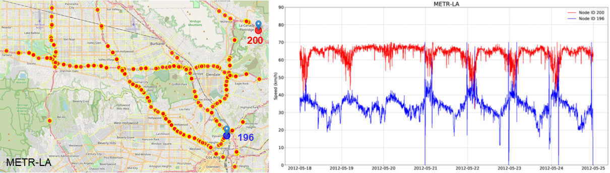
Figure 2. Visualization of METR-LA.

3.1. Grid-Based Traffic Dataset

TaxiBJ. This is taxi in-out flow data published by (Zhang et al., 2017), created from the taxicab GPS data in Beijing from four separate time periods: 2013/7/1-2013/10/30, 2014/3/1-2014/6/30, 2015/3/1-2015/6/30, and 2015/11/1-2016/4/10. Based on the same underlying taxi GPS data (T-Drive), a similar dataset denoted as TaxiBJ-I is created by (Pan et al., 2019).

BikeNYC. This is bike in-out flow data of New York City from 2014/4/1 to 2014/9/30 used by (Zhang et al., 2017). The original bike trip data is published by Citi Bike, NYC’s official bike-sharing system, which includes: trip duration, starting and ending station IDs, and start and end times. Similar datasets BikeNYC-I, BikeNYC-II were used by (Lin et al., 2019) and (Yao et al., 2019) respectively. These two will be used in our experiment due to the larger spatial domain.

TaxiNYC. This is taxi in-out flow data of New York City from 2015/1/1 2015/3/1 used by (Yao et al., 2019). The original taxi trip data is published by the New York City Taxi and Limousine Commission (TLC), that includes pick-up and drop-off dates/times, pick-up and drop-off locations, trip distances, itemized fares, driver-reported passenger counts, etc.

3.2. Graph-Based Traffic Dataset

METR-LA. This is a Los Angeles traffic data published by (Li et al., 2018). The data are collected from 207 highway sensors within 4 months from 2012/3/1 to 2012/6/30. A quite number of studies used this dataset as shown in Table 2. To be intuitive, a data visualization has been made as Fig.2.

PeMS-BAY. This is a traffic flow dataset collected from California Transportation Agencies Performance Measurement System (PeMS). It contains 325 traffic sensors in the Bay Area from 2017/1/1 to 2017/5/31. Massive studies also generate a variety of PeMS datasets by using the same source.

PeMSD7M. This traffic dataset is created and published by (Yu et al., 2018), also collected from PeMS. It covers 228 traffic sensors lasting from 2012/5/1 to 2012/6/30 with a 5-minute sampling rate on weekdays.

Summary. The taxi and bike trip data published by Citi Bike and TLC of New York City and the traffic sensor data from PeMS of California are taken as three trustworthy and wildly-used data sources for traffic prediction. Researchers can easily access the data through the URLs listed in Table 2.

Table 3. Base Technologies Employed for Spatial and Temporal Modeling

Spatial Axis

Temporal Axis

Spatial Axis

Temporal Axis

models

CNN

GCN

Attn.

LSTM

GRU

TCN

Attn.

models

CNN

GCN

Attn.

LSTM

GRU

TCN

Attn.

ST-ResNet(Zhang et al., 2017)

✓

STGCN(Yu et al., 2018)

✓

✓

DMVST-Net(Yao et al., 2018)

✓

✓

GaAN(GGRU)(Zhang et al., 2018)

✓

✓

✓

STDN(Yao et al., 2019)

✓

✓

✓

DCRNN(GCGRU)(Li et al., 2018)

✓

✓

DeepSTN+(Lin et al., 2019)

✓

Multi-graph(Chai et al., 2018)

✓

✓

LSTNet(Lai et al., 2018)

✓

✓

✓

✓

ASTGCN(Guo et al., 2019)

✓

✓

✓

GeoMAN(Liang et al., 2018)

✓

✓

✓

TGCN(Zhao et al., 2019)

✓

✓

TPA-LSTM(Shih et al., 2019)

✓

✓

✓

Graph WaveNet(Wu et al., 2019)

✓

✓

Transformer(Li et al., 2019)

✓

MTGNN(Wu et al., 2020)

✓

✓

ST-MetaNet(Pan et al., 2019)

✓

✓

STGNN(Wang et al., 2020)

✓

✓

✓

✓

GMAN(Zheng et al., 2020)

✓

✓

AGCRN(Bai et al., 2020)

✓

✓

4. Model

Complex spatial and temporal dependencies are the key challenges in urban traffic prediction tasks. Temporally, future prediction depends on the recent observations as well as the past periodical patterns; Spatially, the traffic states in certain mesh-grid or graph-node are affected by the nearby ones as well as distant ones. To capture the temporal dependency, LSTM(Hochreiter and Schmidhuber, 1997) and its simplified variant GRU(Chung et al., 2014) are respectively utilized by the models as shown in Table 3. In parallel with the RNNs, 1D CNN and its enhanced version TCN (Yu and Koltun, 2016) are also employed as the core technology for temporal modeling, and demonstrate the superior time efficiency and matchable effectiveness to LSTM and GRU.

On the other hand, to capture the spatial dependency, grid-based models simply use the normal convolution operation(LeCun et al., 1998) thanks to the natural euclidean property of grid spacing; graph-based models leverage the graph convolution in non-euclidean space (Defferrard et al., 2016; Kipf and Welling, 2017) by involving the adjacency relation $A\in$ $\mathbb{R}^{N*N}$ between each pair of spatial units. Meanwhile, attention mechanism(Vaswani et al., 2017) also known as Transformer has rapidly taken over the AI community from natural language (GPT-3) to vision since 2020. Thus, attention is also introduced as base technology for modeling both spatial and temporal dependencies.

We select the most representative models in Table 1 and summarize the base technologies employed by each model for spatial and temporal modeling as Table 3. On the other hand, for better understanding, we simplify and plot the network architectures in a unified manner for five grid-based models including ST-ResNet(Zhang et al., 2017), DMVST-Net(Yao et al., 2018), Periodic-CRN(PCRN)(Zonoozi et al., 2018), STDN(Yao et al., 2019), and DeepSTN+(Lin et al., 2019) as Fig.3, and five graph-based models, namely STGCN(Yu et al., 2018), DCRNN(Li et al., 2018), Graph WaveNet(Wu et al., 2019), ASTGCN(Guo et al., 2019), and GMAN(Zheng et al., 2020) as Fig.4. Through Fig.3$\sim$4, we can easily understand how the spatial and temporal modules listed in Table 3 are assembled to form an integrated model.

Moreover, we describe how the employed technologies are evolving along the spatial and temporal axis for both grid-based and graph-based models in the next two subsections. Note that the multivariate time-series (MTS) models such as LSTNet(Lai et al., 2018), TPA-LSTM(Shih et al., 2019), GeoMAN(Liang et al., 2018), and Transformer(Li et al., 2019) are also gradually evolving along the spatial and temporal axis. From the spatial perspective, they focus on correlation/dependence between variates; from the temporal perspective, they aim to utilize the periodic patterns occurred in time series. But due to space limitations, we don’t expand the details of those MTS models in this paper.

4.1. Roadmap for Grid-Based Model

ST-ResNet(Zhang et al., 2017) is the earliest and the most representative grid-based deep learning method for traffic in-out flow prediction. It converts 4D tensor ($T$,$H$,$W$,$C$) into 3D tensor ($H$,$W$,$T$*$C$) by concatenating the channels at each time step so that CNN can be used to capture spatial dependency similarly to an image. Then, it creatively proposes a set of temporal features called $Closeness$, $Period$, and $Trend$, which correspond to the most recent observations, daily periodicity, and weekly trend respectively. Intuitively, the three parts of the features can be represented by:

$X^{Closeness}$ = [$X_{t-l_{c}}$, $X_{t-(l_{c}-1)}$, …, $X_{t-1}$]

$X^{Period}$ = [$X_{t-l_{p}\times s_{p}}$, $X_{t-(l_{p}-1)\times s_{p}}$, …, $X_{t-s_{p}}$]

$X^{Trend}$ = [$X_{t-l_{q}\times s_{q}}$, $X_{t-(l_{q}-1)\times s_{q}}$, …, $X_{t-s_{q}}$]

where $l_{c}$, $l_{p}$, $l_{q}$ are the sequence length of {$Closeness$, $Period$, $Trend$}, $s_{p}$ and $s_{q}$ are the time span of $Period$ and $Trend$, the $Closeness$ span $s_{c}$ is equal to 1 by default. This feature is not only inherited by the later grid-based models including STDN(Yao et al., 2019) and DeepSTN+(Lin et al., 2019), but also some graph-based models like ASTGCN(Guo et al., 2019), which is still regarded as the state-of-the-art temporal feature by now. To capture the long-range spatial dependency between mesh-grids, it employs Residual Learning to construct deep enough CNN networks. Additionally, it further utilizes external information including weather, event, and metadata(i.e. DayOfWeek, WeekdayOrWeekend) to auxiliarily enhance spatiotemporal modeling.

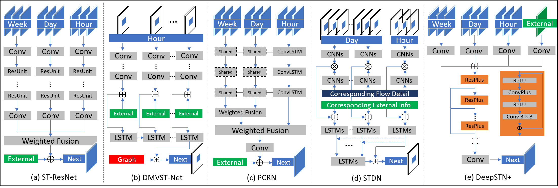
Figure 3. Architectures of Representative Grid-Based Models.

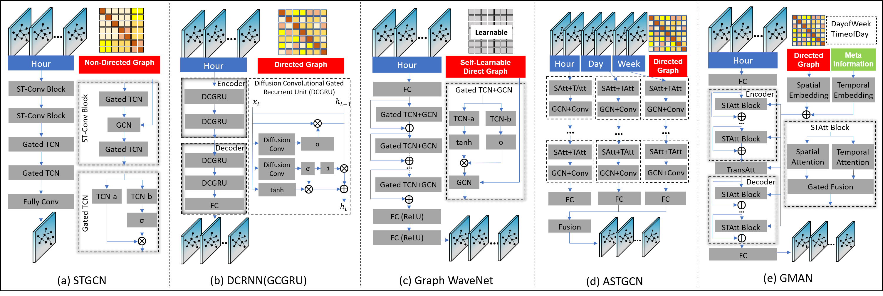
Figure 4. Architectures of Representative Graph-Based Models.

Improvement along Spatial Axis. Different from ST-ResNet that takes the entire mesh-grids as input, DMVST-Net(Yao et al., 2018) and STDN(Yao et al., 2019) take one grid and its surrounding grids (i.e. $S$$\times$$S$ region) as input, thus a local CNN is enough to capture spatial dependency only among nearby grids. For the global spatial dependency, DMVST-Net introduces a weighted graph as an extra input, where nodes are the grids, and each edge represents the similarity of two time-series values (i.e. historical taxi demand) between any two grids. The graph will be manually embedded into a feature vector so that it can be concatenated with the other part. Through this, DMVST-Net gains the ability to capture long-range spatial dependency. Furthermore, STDN and (Zhang et al., 2019; Jiang et al., 2019) consider the local flow information (i.e. flow from one central grid to its surrounding $S$$\times$$S$ grids) to facilitate predicting the traffic volume in the central grid, which is implemented with a flow gating mechanism in STDN and multitask learning in (Zhang et al., 2019; Jiang et al., 2019). DeepSTN+ (Lin et al., 2019) uses Point-Of-Interest (POI) data as external information (e.g., office/residential/shopping area) to take the influence of location function on the crowd/traffic flow into consideration.

Improvement along Temporal Axis. One major drawback of ST-ResNet is it does not explicitly handle the temporal axis, because it forces the video-like tensor ($T$,$H$,$W$,$C$) to be converted into an image-like tensor ($H$,$W$,$T$*$C$). To address this, DMVST-Net and STDN employ LSTM to connect with a separate and unshared CNN for each timestamp. STDN further considers the temporal shifting problem about periodicity (i.e. traffic data is not strictly periodic) and designs a Periodically Shifted Attention Mechanism to solve the issue. Specifically, it sets a small time window to collect $Q$ time intervals right before and after the currently-predicting one. And the attention is used to obtain a weighted average representation $h$ from the $Q$ representations {$h_{1}$, $h_{2}$, $...$, $h_{Q}$} generated by LSTM. To this end, LSTM, and CNN work together to separately and sequentially model the spatial and temporal dependency. Convolutional LSTM (Xingjian et al., 2015) extends the fully connected LSTM (FC-LSTM) to have convolutional structures in both the input-to-state and state-to-state transitions and achieves a lot of successes on video modeling tasks. Motivated by this, ConvLSTM and its variant ConvGRU are utilized by (Zonoozi et al., 2018; Yuan et al., 2018; Jiang et al., 2019) to simultaneously capture the spatial and temporal dependency.

Table 4. Performance Evaluation for Single-Step Prediction on Grid-Based Traffic Datasets

	TaxiBJ			BikeNYC-I			BikeNYC-II			TaxiNYC
Model	RMSE	MAE	MAPE	RMSE	MAE	MAPE	RMSE	MAE	MAPE	RMSE	MAE	MAPE
HistoricalAverage	45.004	24.475	8.04%	15.676	4.882	5.45%	4.874	1.500	3.30%	21.535	7.121	4.56%
CopyLastStep	23.609	13.372	6.20%	14.152	4.344	5.01%	4.999	1.606	3.50%	18.660	6.497	4.91%
CNN(LeCun et al., 1998)	23.550	13.797	8.46%	12.064	4.088	5.82%	4.511	1.574	3.98%	16.741	6.884	8.08%
ConvLSTM(Xingjian et al., 2015)	19.247	10.816	5.61%	6.616	2.412	3.90%	3.174	1.133	2.90%	12.143	4.811	5.16%
ST-ResNet(Zhang et al., 2017)	18.702	10.493	5.19%	6.106	2.360	3.72%	3.191	1.169	2.86%	11.553	4.535	4.32%
DMVST-Net(Yao et al., 2018)	20.389	11.832	5.99%	7.990	2.833	3.93%	3.521	1.287	2.97%	13.605	4.928	4.49%
PCRN(Zonoozi et al., 2018)	18.629	10.432	5.45%	6.680	2.351	3.63%	3.149	1.107	2.78%	12.027	4.606	4.62%
DeepSTN+(Lin et al., 2019)	18.141	10.126	5.14%	6.205	2.489	3.48%	3.205	1.245	2.80%	11.420	4.441	4.45%
STDN(Yao et al., 2019)	17.826	9.901	4.81%	5.783	2.410	3.35%	3.004	1.167	2.67%	11.252	4.474	4.09%

Table 5. Performance Evaluation for Multi-Step Prediction on Graph-Based Traffic Datasets

		3 Steps / 15 Minutes Ahead			6 Steps / 30 Minutes Ahead			12 Steps / 60 Minutes Ahead
Dataset	Model	RMSE	MAE	MAPE	RMSE	MAE	MAPE	RMSE	MAE	MAPE
METR-LA	HistoricalAverage	14.737	11.013	23.34%	14.737	11.010	23.34%	14.736	11.005	23.33%
	CopyLastSteps	14.215	6.799	16.73%	14.214	6.799	16.73%	14.214	6.798	16.72%
	LSTNet(Lai et al., 2018)	8.067	3.914	9.27%	10.181	5.219	12.22%	11.890	6.335	15.38%
	STGCN(Yu et al., 2018)	7.918	3.469	8.57%	9.948	4.263	10.70%	11.813	5.079	13.09%
	DCRNN(Li et al., 2018)	7.509	3.261	8.00%	9.543	4.021	10.12%	11.854	5.080	13.08%
	Graph WaveNet(Wu et al., 2019)	7.512	3.204	7.62%	9.445	3.922	9.52%	11.485	4.848	11.93%
	ASTGCN(Guo et al., 2019)	7.977	3.624	9.13%	10.042	4.514	11.57%	12.092	5.776	14.85%
	GMAN(Zheng et al., 2020)	8.869	4.139	10.88%	9.917	4.517	11.77%	11.910	5.475	14.10%
	MTGNN(Wu et al., 2020)	7.707	3.277	8.02%	9.625	3.999	10.00%	11.624	4.867	12.17%
	AGCRN(Bai et al., 2020)	7.558	3.292	8.17%	9.499	4.016	10.16%	11.502	4.901	12.43%
PeMS-BAY	HistoricalAverage	6.687	3.333	8.10%	6.686	3.333	8.10%	6.685	3.332	8.10%
	CopyLastSteps	7.022	3.052	6.84%	7.016	3.049	6.84%	7.05	3.044	6.83%
	LSTNet(Lai et al., 2018)	3.224	1.643	3.47%	4.375	2.383	5.04%	5.515	2.974	6.86%
	STGCN(Yu et al., 2018)	2.827	1.327	2.79%	3.887	1.698	3.81%	4.748	2.055	5.02%
	DCRNN(Li et al., 2018)	2.867	1.377	2.96%	3.905	1.726	3.97%	4.798	2.091	4.99%
	Graph WaveNet(Wu et al., 2019)	2.759	1.322	2.78%	3.737	1.660	3.75%	4.562	1.991	4.75%
	ASTGCN(Guo et al., 2019)	3.057	1.435	3.25%	4.066	1.795	4.40%	4.770	2.103	5.30%
	GMAN(Zheng et al., 2020)	4.219	1.802	4.47%	4.143	1.794	4.40%	5.034	2.186	5.29%
	MTGNN(Wu et al., 2020)	2.849	1.334	2.84%	3.800	1.658	3.77%	4.491	1.950	4.59%
	AGCRN(Bai et al., 2020)	2.856	1.354	2.94%	3.818	1.670	3.84%	4.570	1.964	4.69%
PEMSD7M	HistoricalAverage	7.077	3.917	9.90%	7.083	3.920	9.92%	7.095	3.925	9.95%
	CopyLastSteps	9.591	5.021	12.33%	9.594	5.022	12.33%	9.597	5.024	12.34%
	LSTNet(Lai et al., 2018)	4.308	2.423	5.73%	8.951	5.132	12.22%	10.881	6.624	16.72%
	STGCN(Yu et al., 2018)	4.051	2.124	5.02%	5.532	2.783	6.96%	6.695	3.374	8.74%
	DCRNN(Li et al., 2018)	4.143	2.213	5.33%	5.679	2.907	7.41%	7.138	3.670	9.81%
	Graph WaveNet(Wu et al., 2019)	3.992	2.130	5.00%	5.332	2.715	6.75%	6.431	3.266	8.47%
	ASTGCN(Guo et al., 2019)	4.257	2.340	5.83%	5.506	2.992	7.69%	6.587	3.572	9.48%
	GMAN(Zheng et al., 2020)	5.711	2.877	7.25%	6.171	3.084	7.77%	7.897	3.988	10.02%
	MTGNN(Wu et al., 2020)	4.032	2.120	5.02%	5.373	2.687	6.70%	6.496	3.204	8.24%
	AGCRN(Bai et al., 2020)	4.073	2.167	5.19%	5.479	2.769	6.89%	6.733	3.358	8.55%

4.2. Roadmap for Graph-Based Model

STGCN(Yu et al., 2018) is one of the earliest models that use graph neural networks to predict traffic flow. Temporally, instead of RNN, it uses TCN (Yu and Koltun, 2016) with a gated mechanism as shown in Fig.4 to capture the dependency only from $Closeness$ features. Spatially, it applies two spectral graph convolution, ChebyNet(Defferrard et al., 2016) and 1st-order approximation of ChebyNet (Kipf and Welling, 2017). TCN and GCN are stacked together as an ST-Conv block to sequentially do the spatial and temporal modeling. One major limitation of STGCN is that it uses a symmetrical adjacency matrix (i.e., undirected graph) that considers the euclidean distance between two road sensors. Thus it is difficult to model the difference of the two-way traffic flow in one road. DCRNN (Li et al., 2018) is another pioneer to utilize graph convolution for traffic flow prediction. In contrast to the spectral convolution in STGCN, DCRNN applies a spatial graph convolution called Diffusion Convolution implemented with bidirectional random walks on a directed graph (i.e., non-symmetric adjacent matrix), so that it can capture the spatial influence from both the upstream and the downstream traffic flows. For the temporal axis, similar to ConvLSTM, it replaces the normal matrix multiplication in GRU with the proposed diffusion convolution, then a Diffusion Convolution Gated Recurrent Unit (DCGRU) is assembled that can simultaneously do the spatial and temporal modeling. With this DCGRU, it further implements an encoder-decoder structure to enable the multi-step-to-multi-step prediction. Inspired by STGCN and DCRNN, massive graph-based traffic models have been proposed as summarized in Table 1.

Improvement along Temporal Axis. For the temporal feature, ASTGCN(Guo et al., 2019) inherits $Closeness$, $Period$, and $Trend$ from ST-ResNet, and improves STGCN that only takes $Closeness$. Besides, STSGCN(Song et al., 2020) constructs a localized temporal graph by connecting all nodes with themselves at the previous and the next steps, updating the adjacency matrix from $A$$\in$$\mathbb{R}^{N*N}$ to $A^{\prime}$$\in$$\mathbb{R}^{3N*3N}$, then only uses GCN to simultaneously do the spatial and temporal modeling. On the other hand, to get better ability of temporal modeling, T-GCN(Zhao et al., 2019) and TGC-LSTM(Cui et al., 2019) respectively use GRU and LSTM instead of TCN to improve STGCN; GCGA(Yu and Gu, 2019) combines Generative Adversarial Network(GAN) and Autoencoder with GCN; STGNN(Wang et al., 2020) adopts transformer (attention) for better global/long-term temporal modeling; STG2Seq(Bai et al., 2019) utilized GCN for temporal modeling, which is an interesting attempt.

Improvement along Spatial Axis. A lot of effort has been put on the spatial axis, that is the graph. (1) From single-graph to multi-graph. STGCN and DCRNN only use a single graph, directed or non-directed, to describe the spatial relationship. However, multimodal correlations and compound spatial dependencies exist among regions. Therefore, a series of researches elevate single-graph to multi-graph. For instance, (Chai et al., 2018) and ST-MGCN(Geng et al., 2019) consider spatial proximity, functional similarity, and road connectivity as mutli-graph, and so as T-MGCN(Lv et al., 2020); H-STGCN(Dai et al., 2020) takes travel time correlation matrix and shortest-path distance matrix as compound matrix; MRA-BGCN(Chen et al., 2020) builds the node-wise graph according to the road network distance, and the edge-wise graph according to the connectivity and competition. (2) From static graph to adaptive graph. Graph WaveNet(Wu et al., 2019), TGC-LSTM(Cui et al., 2019), and AGCRN(Bai et al., 2020) adopt adaptive/learnable graph rather than a static one used in STGCN and DCRNN; DGCNN(Diao et al., 2019) proposes dynamic Laplacian matrix learning through tensor decomposition; SLCNN(Zhang et al., 2020a) designs Structure Learning Convolution (SLC) to dynamically learn the global/local graph structure. In addition to the above, attention-augmented GCN also demonstrated better performance in terms of spatial modeling in GaAN(Zhang et al., 2018), ASTGCN, and GMAN(Zheng et al., 2020).

5. Evaluation

5.1. Setting

Towards the benchmark tasks listed in Section 2, we pick up some representative models and conduct comprehensive evaluations about their actual performances. Besides the deep models, we also implement two naive baselines as follows: (1) HistoricalAverage(HA). We average the corresponding values from historical days as the prediction result; (2) CopyLastStep(s). We directly copy the last one or multiple steps as the prediction result. Our experiments were performed on a GPU server with four GeForce GTX 2080Ti graphics cards. As a benchmark evaluation, the following settings are kept the same for each model. The observation step is set to 6 for grid-based models, while the observation and prediction step are both set to 12 for graph-based models. The data ratio for training, validation, and testing is set as 7:1:2. Adam was set as the default optimizer, where the learning rate was set to 0.001 and the batch size was set to 64 by default. Mean Absolute Error is uniformly used as the loss function. The training algorithm would either be early-stopped if the validation error was converged within 10 epochs or be stopped after 200 epochs, and the best model on validation data would be saved. Root Mean Square Error (RMSE), Mean Absolute Error (MAE), and Mean Absolute Percentage Error (MAPE) are used as metrics, where zero values will be ignored.

5.2. Effectiveness Evaluation

The evaluation of grid-based models for single-step prediction is shown in Table 4; the evaluation of graph-based models for multi-step prediction is shown in Table 5.

Evaluation for Grid-Based Model: Table 4 shows that the state-of-the-art models did have advantages over the baselines (HA $\sim$ ConvLSTM). In particular, STDN showed better performances in general, PCRN and DeepSTN+ achieved the lowest MAE on BikeNYC-I and TaxiNYC respectively. None of these grid-based models could be acknowledged as a dominant one at the current stage. Through the experiment, we find that their main limitations are as follows: (1) ST-ResNet converts the video-like data to high-dimensional image-like data and uses a simple fusion-mechanism to handle different types of temporal dependency; (2) through the experiment, it was found PCRN took more epochs to converge and tended to cause overfitting; (3) DMVST-Net and STDN use local CNN to take grid (pixel) as computation unit, resulting in long training time; (4) DeepSTN+ utilized a fully-connected layer in $ConvPlus$ block, which would result in a big number of parameters on TaxiBJ; (4) Multitask Learning model(Zhang et al., 2019; Jiang et al., 2019) needs multiple data sources as the inputs, which hinders the applicability.

Evaluation for Graph-Based Model: Table 5 compares the prediction performances of our selected models at 15 minutes, 30 minutes, 60 minutes ahead on METR-LA, PeMS-BAY, PEMSD7M datasets. Through Table 5, we can find that: (1) Despite the effect of time-series model LSTNet in short-term prediction, its performance would deteriorate as the horizon gets longer; (2) Almost all of the graph-based models achieved better performance than traditional methods and time-series models on all metrics, which proved that the addition of spatial information would bring substantial performance improvements; (3) Although the models’ performances depended more or less on the dataset, the scores of DCRNN, Graph WaveNet, and MTGNN on all datasets ranked in the top 3, which also proved their robustness and versatility in traffic prediction tasks; (4) GMAN was found more prone to overfitting, due to which its performances on all three datasets were not as good as LSTNet; This is probably because GMAN adopted a global attention mechanism to capture the spatial dependency between each pair of nodes; (5) MTGNN and GraphWaveNet got most of the highest scores on different datasets and metrics. The self-adaptive/learnable graph demonstrated its great effectiveness for traffic prediction.

Figure 5. Case Study on Graph-Based Datasets.

Case Study: We randomly selected one day (24 hours) and one sensor (node) from the three datasets (i.e., METR-LA, PEMS-BAY, and PEMSD7M) and plotted the time series of the ground truth and the predictions as Fig.5. To make the time-series chart clear, in addition to the ground truth, we only plot the prediction results of LSTNet, DCRNN, and Graph WaveNet instead of all of the models listed in Table 5. Through Fig.5, we can observe that: (1) All of the three models could learn the peak and valley trend on all three datasets; (2) The graph-based models DCRNN and Graph WaveNet always outperformed the time-series model LSTNet, which proved the excellent performance of GCN in capturing spatial correlation and dependency; (3) Time lag could be observed on all of the three prediction results, especially when violent fluctuations occur in the original time series such as 2012/6/20 21:00 in PEMSD7M. This problem will be magnified in the longer-term forecast like 60 minutes lead time. Despite this, the graph-based models still show better performance in terms of volatility prediction errors, which further confirmed the effectiveness and robustness of GCN in traffic prediction.

Figure 6. Efficiency Summary.

5.3. Efficiency Evaluation

Besides comparing the effectiveness of these deep models, we also provide an analysis of their efficiency. The space complexity and time complexity of these approaches are significant for their future application, so we exhibit the number of the trainable parameters and training time of each model through bar charts Fig.6.

Evaluation for Grid-Based Model: From Fig.6-(a) and Fig.6-(b), we can observe that: (1) the parameter numbers of DeepSTN+ and STDN are more than other models, especially DeepSTN+, which captures the citywide spatial correlation by utilizing fully connected layer; (2) ST-ResNet has the fewest trainable parameters, and demonstrates its superiority to other models in terms of space complexity; (3) The training time of STDN and DMVST is longer than other models because they utilize the LSTM to capture the temporal dependency and take each mesh-grid as the computation unit rather than the entire mesh.

Evaluation for Graph-Based Model: From Fig.6-(c) and Fig.6-(d), we can conclude that: (1) STGCN and GMAN have relatively lower space complexity than others; (2) AGCRN and DCRNN need more parameters than other models because they are based on RNNs; (3) On PEMSBAY, the parameter numbers of ASTGCN and MTGNN dramatically increase. The reason for this is those two models have more GNN layers and they are more sensitive to the node number; (4) The training time of GMAN on PEMSBAY outdistances other models because it applies a global attention mechanism to the entire graph (nodes). In summary, TCN-based models like STGCN and Graph WaveNet have higher computation efficiency.

6. Availability and Usability

DL-Traff is already available at GitHub as the following two repositories under the MIT License: one is for grid-based datasets/models https://github.com/deepkashiwa20/DL-Traff-Grid, and another is for graph-based datasets/models https://github.com/deepkashiwa20/DL-Traff-Graph. It is implemented with Python and the most popular deep learning frameworks: Keras(Chollet, 2015) on TensorFlow(Abadi et al., 2015) and PyTorch(Paszke et al., 2019). Fig.7 shows a use case by taking DCRNN model on METR-LA dataset as an example. To run the benchmark, the repository should be cloned locally and a conda environment with the necessary dependencies should be created. The directory is structured in a flat style and only with two levels. The traffic datasets are stored in DATA directories (e.g., METRLA), and the python files are put in workDATA directories (e.g., workMETRLA). Entering the work directory for a certain dataset, we can find MODEL class file (e.g., DCRNN.py) and its corresponding running program named pred_MODEL.py (e.g., pred_DCRNN.py). We can run “python MODEL.py” to simply check the model architecture without feeding the training data and run “python pred_MODEL.py” to train and test the model. Additionally, Param.py file contains a variety of hyper-parameters as described in Section 5.1 that allow the experiment to be customized in a unified way. Metrics.py file contains the metric functions listed in Section 5.1. Utils.py file integrates a set of supporting functions such as pickle file reader and self-defined loss function. More details about the usability and implementation can be found at GitHub.

Figure 7. Illustration of The Use Case for DL-Traff.

7. Conclusion

In this paper, we first survey the deep learning models as well as the widely used datasets for urban traffic prediction. Then we build a standard benchmark to comprehensively evaluate the deep traffic models on the selected open datasets. The survey and the benchmark combine together to form our study called DL-Traff, which is already available at https://github.com/deepkashiwa20/DL-Traff-Grid and https://github.com/deepkashiwa20/DL-Traff-Graph. With DL-Traff, we hope to deliver a useful and timely resource to researchers in AI and data science community.

References

- (1)
- Abadi et al. (2015) Martín Abadi, Ashish Agarwal, Paul Barham, Eugene Brevdo, Zhifeng Chen, Craig Citro, Greg S. Corrado, Andy Davis, Jeffrey Dean, Matthieu Devin, Sanjay Ghemawat, Ian Goodfellow, Andrew Harp, Geoffrey Irving, Michael Isard, Yangqing Jia, Rafal Jozefowicz, Lukasz Kaiser, Manjunath Kudlur, Josh Levenberg, Dan Mané, Rajat Monga, Sherry Moore, Derek Murray, Chris Olah, Mike Schuster, Jonathon Shlens, Benoit Steiner, Ilya Sutskever, Kunal Talwar, Paul Tucker, Vincent Vanhoucke, Vijay Vasudevan, Fernanda Viégas, Oriol Vinyals, Pete Warden, Martin Wattenberg, Martin Wicke, Yuan Yu, and Xiaoqiang Zheng. 2015. TensorFlow: Large-Scale Machine Learning on Heterogeneous Systems. http://tensorflow.org/ Software available from tensorflow.org.
- Bai et al. (2019) Lei Bai, Lina Yao, Salil Kanhere, Xianzhi Wang, Quan Sheng, et al. 2019. Stg2seq: Spatial-temporal graph to sequence model for multi-step passenger demand forecasting. In IJCAI. 1981–1987.
- Bai et al. (2020) Lei Bai, Lina Yao, Can Li, Xianzhi Wang, and Can Wang. 2020. Adaptive Graph Convolutional Recurrent Network for Traffic Forecasting. In 34th Conference on Neural Information Processing Systems.
- Chai et al. (2018) Di Chai, Leye Wang, and Qiang Yang. 2018. Bike flow prediction with multi-graph convolutional networks. In Proceedings of the 26th ACM SIGSPATIAL International Conference on Advances in Geographic Information Systems. 397–400.
- Chen et al. (2020) Weiqi Chen, Ling Chen, Yu Xie, Wei Cao, Yusong Gao, and Xiaojie Feng. 2020. Multi-range attentive bicomponent graph convolutional network for traffic forecasting. In Proceedings of the AAAI Conference on Artificial Intelligence, Vol. 34. 3529–3536.
- Chollet (2015) François Chollet. 2015. keras. https://github.com/fchollet/keras.
- Chung et al. (2014) Junyoung Chung, Caglar Gulcehre, Kyunghyun Cho, and Yoshua Bengio. 2014. Empirical evaluation of gated recurrent neural networks on sequence modeling. In NIPS 2014 Workshop on Deep Learning, December 2014.
- Cui et al. (2019) Zhiyong Cui, Kristian Henrickson, Ruimin Ke, and Yinhai Wang. 2019. Traffic graph convolutional recurrent neural network: A deep learning framework for network-scale traffic learning and forecasting. IEEE Transactions on Intelligent Transportation Systems (2019).
- Dai et al. (2020) Rui Dai, Shenkun Xu, Qian Gu, Chenguang Ji, and Kaikui Liu. 2020. Hybrid Spatio-Temporal Graph Convolutional Network: Improving Traffic Prediction with Navigation Data. In Proceedings of the 26th ACM SIGKDD International Conference on Knowledge Discovery & Data Mining. 3074–3082.
- Defferrard et al. (2016) Michaël Defferrard, Xavier Bresson, and Pierre Vandergheynst. 2016. Convolutional neural networks on graphs with fast localized spectral filtering. In Advances in neural information processing systems. 3844–3852.
- Diao et al. (2019) Zulong Diao, Xin Wang, Dafang Zhang, Yingru Liu, Kun Xie, and Shaoyao He. 2019. Dynamic spatial-temporal graph convolutional neural networks for traffic forecasting. In Proceedings of the AAAI Conference on Artificial Intelligence, Vol. 33. 890–897.
- Geng et al. (2019) Xu Geng, Yaguang Li, Leye Wang, Lingyu Zhang, Qiang Yang, Jieping Ye, and Yan Liu. 2019. Spatiotemporal multi-graph convolution network for ride-hailing demand forecasting. In 2019 AAAI Conference on Artificial Intelligence (AAAI’19).
- Guo et al. (2020) Kan Guo, Yongli Hu, Zhen Qian, Yanfeng Sun, Junbin Gao, and Baocai Yin. 2020. Dynamic Graph Convolution Network for Traffic Forecasting Based on Latent Network of Laplace Matrix Estimation. IEEE Transactions on Intelligent Transportation Systems (2020).
- Guo et al. (2019) Shengnan Guo, Youfang Lin, Ning Feng, Chao Song, and Huaiyu Wan. 2019. Attention based spatial-temporal graph convolutional networks for traffic flow forecasting. In Proceedings of the AAAI Conference on Artificial Intelligence, Vol. 33. 922–929.
- Hoang et al. (2016) Minh X Hoang, Yu Zheng, and Ambuj K Singh. 2016. Forecasting citywide crowd flows based on big data. ACM SIGSPATIAL (2016).
- Hochreiter and Schmidhuber (1997) Sepp Hochreiter and Jürgen Schmidhuber. 1997. Long short-term memory. Neural computation 9, 8 (1997), 1735–1780.
- Huang et al. (2014) Wenhao Huang, Guojie Song, Haikun Hong, and Kunqing Xie. 2014. Deep architecture for traffic flow prediction: Deep belief networks with multitask learning. IEEE Transactions on Intelligent Transportation Systems 15, 5 (2014), 2191–2201.
- Jiang et al. (2019) Renhe Jiang, Xuan Song, Dou Huang, Xiaoya Song, Tianqi Xia, Zekun Cai, Zhaonan Wang, Kyoung-Sook Kim, and Ryosuke Shibasaki. 2019. DeepUrbanEvent: A System for Predicting Citywide Crowd Dynamics at Big Events. In Proceedings of the 25th ACM SIGKDD International Conference on Knowledge Discovery & Data Mining. ACM, 2114–2122.
- Kipf and Welling (2017) Thomas N Kipf and Max Welling. 2017. Semi-Supervised Classification with Graph Convolutional Networks. (2017).
- Lai et al. (2018) Guokun Lai, Wei-Cheng Chang, Yiming Yang, and Hanxiao Liu. 2018. Modeling long-and short-term temporal patterns with deep neural networks. In The 41st International ACM SIGIR Conference on Research & Development in Information Retrieval. 95–104.
- LeCun et al. (1998) Yann LeCun, Léon Bottou, Yoshua Bengio, and Patrick Haffner. 1998. Gradient-based learning applied to document recognition. Proc. IEEE 86, 11 (1998), 2278–2324.
- Li et al. (2019) Shiyang Li, Xiaoyong Jin, Yao Xuan, Xiyou Zhou, Wenhu Chen, Yu-Xiang Wang, and Xifeng Yan. 2019. Enhancing the locality and breaking the memory bottleneck of transformer on time series forecasting. In Advances in Neural Information Processing Systems. 5243–5253.
- Li et al. (2018) Yaguang Li, Rose Yu, Cyrus Shahabi, and Yan Liu. 2018. Diffusion Convolutional Recurrent Neural Network: Data-Driven Traffic Forecasting. In International Conference on Learning Representations.
- Liang et al. (2018) Yuxuan Liang, Songyu Ke, Junbo Zhang, Xiuwen Yi, and Yu Zheng. 2018. Geoman: Multi-level attention networks for geo-sensory time series prediction. In IJCAI. 3428–3434.
- Lin et al. (2019) Ziqian Lin, Jie Feng, Ziyang Lu, Yong Li, and Depeng Jin. 2019. DeepSTN+: Context-aware Spatial-Temporal Neural Network for Crowd Flow Prediction in Metropolis. AAAI.
- Lv et al. (2020) Mingqi Lv, Zhaoxiong Hong, Ling Chen, Tieming Chen, Tiantian Zhu, and Shouling Ji. 2020. Temporal multi-graph convolutional network for traffic flow prediction. IEEE Transactions on Intelligent Transportation Systems (2020).
- Lv et al. (2014) Yisheng Lv, Yanjie Duan, Wenwen Kang, Zhengxi Li, and Fei-Yue Wang. 2014. Traffic flow prediction with big data: a deep learning approach. IEEE Transactions on Intelligent Transportation Systems 16, 2 (2014), 865–873.
- Ma et al. (2017) Xiaolei Ma, Zhuang Dai, Zhengbing He, Jihui Ma, Yong Wang, and Yunpeng Wang. 2017. Learning traffic as images: a deep convolutional neural network for large-scale transportation network speed prediction. Sensors 17, 4 (2017), 818.
- Ma et al. (2015) Xiaolei Ma, Zhimin Tao, Yinhai Wang, Haiyang Yu, and Yunpeng Wang. 2015. Long short-term memory neural network for traffic speed prediction using remote microwave sensor data. Transportation Research Part C: Emerging Technologies 54 (2015), 187–197.
- Pan et al. (2019) Zheyi Pan, Yuxuan Liang, Weifeng Wang, Yong Yu, Yu Zheng, and Junbo Zhang. 2019. Urban Traffic Prediction from Spatio-Temporal Data Using Deep Meta Learning. In Proceedings of the 25th ACM SIGKDD International Conference on Knowledge Discovery & Data Mining. ACM, 1720–1730.
- Paszke et al. (2019) Adam Paszke, Sam Gross, Francisco Massa, Adam Lerer, James Bradbury, Gregory Chanan, Trevor Killeen, Zeming Lin, Natalia Gimelshein, Luca Antiga, Alban Desmaison, Andreas Kopf, Edward Yang, Zachary DeVito, Martin Raison, Alykhan Tejani, Sasank Chilamkurthy, Benoit Steiner, Lu Fang, Junjie Bai, and Soumith Chintala. 2019. PyTorch: An Imperative Style, High-Performance Deep Learning Library. In Advances in Neural Information Processing Systems 32, H. Wallach, H. Larochelle, A. Beygelzimer, F. d'Alché-Buc, E. Fox, and R. Garnett (Eds.). Curran Associates, Inc., 8024–8035. http://papers.neurips.cc/paper/9015-pytorch-an-imperative-style-high-performance-deep-learning-library.pdf
- Shih et al. (2019) Shun-Yao Shih, Fan-Keng Sun, and Hung-yi Lee. 2019. Temporal pattern attention for multivariate time series forecasting. Machine Learning 108, 8-9 (2019), 1421–1441.
- Song et al. (2020) Chao Song, Youfang Lin, Shengnan Guo, and Huaiyu Wan. 2020. Spatial-Temporal Synchronous Graph Convolutional Networks: A New Framework for Spatial-Temporal Network Data Forecasting. In Proceedings of the AAAI Conference on Artificial Intelligence, Vol. 34. 914–921.
- Vaswani et al. (2017) Ashish Vaswani, Noam Shazeer, Niki Parmar, Jakob Uszkoreit, Llion Jones, Aidan N Gomez, Lukasz Kaiser, and Illia Polosukhin. 2017. Attention is All you Need. In NIPS.
- Wang et al. (2017) Dong Wang, Wei Cao, Jian Li, and Jieping Ye. 2017. DeepSD: supply-demand prediction for online car-hailing services using deep neural networks. In 2017 IEEE 33rd International Conference on Data Engineering (ICDE). IEEE, 243–254.
- Wang et al. (2020) Xiaoyang Wang, Yao Ma, Yiqi Wang, Wei Jin, Xin Wang, Jiliang Tang, Caiyan Jia, and Jian Yu. 2020. Traffic Flow Prediction via Spatial Temporal Graph Neural Network. In Proceedings of The Web Conference 2020. 1082–1092.
- Wu et al. (2020) Zonghan Wu, Shirui Pan, Guodong Long, Jing Jiang, Xiaojun Chang, and Chengqi Zhang. 2020. Connecting the dots: Multivariate time series forecasting with graph neural networks. In Proceedings of the 26th ACM SIGKDD International Conference on Knowledge Discovery & Data Mining. 753–763.
- Wu et al. (2019) Zonghan Wu, Shirui Pan, Guodong Long, Jing Jiang, and Chengqi Zhang. 2019. Graph wavenet for deep spatial-temporal graph modeling. In IJCAI. 1907–1913.
- Xingjian et al. (2015) SHI Xingjian, Zhourong Chen, Hao Wang, Dit-Yan Yeung, Wai-Kin Wong, and Wang-chun Woo. 2015. Convolutional LSTM network: A machine learning approach for precipitation nowcasting. In Advances in neural information processing systems. 802–810.
- Yao et al. (2019) Huaxiu Yao, Xianfeng Tang, Hua Wei, Guanjie Zheng, and Zhenhui Li. 2019. Revisiting Spatial-Temporal Similarity: A Deep Learning Framework for Traffic Prediction. In 2019 AAAI Conference on Artificial Intelligence (AAAI’19).
- Yao et al. (2018) Huaxiu Yao, Fei Wu, Jintao Ke, Xianfeng Tang, Yitian Jia, Siyu Lu, Pinghua Gong, Jieping Ye, and Zhenhui Li. 2018. Deep multi-view spatial-temporal network for taxi demand prediction. In Thirty-Second AAAI Conference on Artificial Intelligence.
- Yu et al. (2018) Bing Yu, Haoteng Yin, and Zhanxing Zhu. 2018. Spatio-temporal graph convolutional networks: a deep learning framework for traffic forecasting. In Proceedings of the 27th International Joint Conference on Artificial Intelligence. AAAI Press, 3634–3640.
- Yu and Koltun (2016) Fisher Yu and Vladlen Koltun. 2016. Multi-Scale Context Aggregation by Dilated Convolutions. In ICLR.
- Yu and Gu (2019) James Jian Qiao Yu and Jiatao Gu. 2019. Real-time traffic speed estimation with graph convolutional generative autoencoder. IEEE Transactions on Intelligent Transportation Systems 20, 10 (2019), 3940–3951.
- Yuan et al. (2018) Zhuoning Yuan, Xun Zhou, and Tianbao Yang. 2018. Hetero-ConvLSTM: A Deep Learning Approach to Traffic Accident Prediction on Heterogeneous Spatio-Temporal Data. In Proceedings of the 24th ACM SIGKDD International Conference on Knowledge Discovery & Data Mining. ACM, 984–992.
- Zhang et al. (2018) Jiani Zhang, Xingjian Shi, Junyuan Xie, Hao Ma, Irwin King, and Dit Yan Yeung. 2018. GaAN: Gated Attention Networks for Learning on Large and Spatiotemporal Graphs. In 34th Conference on Uncertainty in Artificial Intelligence 2018, UAI 2018.
- Zhang et al. (2017) Junbo Zhang, Yu Zheng, and Dekang Qi. 2017. Deep Spatio-Temporal Residual Networks for Citywide Crowd Flows Prediction.. In AAAI. 1655–1661.
- Zhang et al. (2016) Junbo Zhang, Yu Zheng, Dekang Qi, Ruiyuan Li, and Xiuwen Yi. 2016. DNN-based prediction model for spatio-temporal data. In Proceedings of the 24th ACM SIGSPATIAL International Conference on Advances in Geographic Information Systems. ACM, 92.
- Zhang et al. (2019) Junbo Zhang, Yu Zheng, Junkai Sun, and Dekang Qi. 2019. Flow Prediction in Spatio-Temporal Networks Based on Multitask Deep Learning. IEEE Transactions on Knowledge and Data Engineering (2019).
- Zhang et al. (2020a) Qi Zhang, Jianlong Chang, Gaofeng Meng, Shiming Xiang, and Chunhong Pan. 2020a. Spatio-temporal graph structure learning for traffic forecasting. In Proceedings of the AAAI Conference on Artificial Intelligence, Vol. 34. 1177–1185.
- Zhang et al. (2020b) Yingxue Zhang, Yanhua Li, Xun Zhou, Xiangnan Kong, and Jun Luo. 2020b. Curb-GAN: Conditional Urban Traffic Estimation through Spatio-Temporal Generative Adversarial Networks. In Proceedings of the 26th ACM SIGKDD International Conference on Knowledge Discovery & Data Mining. 842–852.
- Zhao et al. (2019) Ling Zhao, Yujiao Song, Chao Zhang, Yu Liu, Pu Wang, Tao Lin, Min Deng, and Haifeng Li. 2019. T-gcn: A temporal graph convolutional network for traffic prediction. IEEE Transactions on Intelligent Transportation Systems (2019).
- Zheng et al. (2020) Chuanpan Zheng, Xiaoliang Fan, Cheng Wang, and Jianzhong Qi. 2020. Gman: A graph multi-attention network for traffic prediction. In Proceedings of the AAAI Conference on Artificial Intelligence, Vol. 34. 1234–1241.
- Zonoozi et al. (2018) Ali Zonoozi, Jung-jae Kim, Xiao-Li Li, and Gao Cong. 2018. Periodic-CRN: A Convolutional Recurrent Model for Crowd Density Prediction with Recurring Periodic Patterns.. In IJCAI. 3732–3738.