Light rings and long-lived modes in quasiblack hole spacetimes

Abstract

It has been argued that ultracompact objects, which possess light rings but no horizons, may be unstable against gravitational perturbations. To test this conjecture, we revisit the quasi-black hole solutions, a family of horizonless spacetimes whose limit is the extremal Reissner-Nordström black hole. We find a critical parameter at which the light rings just appear. We then calculate the quasinormal modes of the quasi-black holes. Both the WKB result and the numerical result show that long-lived modes survive for the range where light rings exist, indicating that horizonless spacetimes with light rings are unstable. Our work provides a strong and explicit example that light rings could be direct observational evidence for black holes.

Department of Physics, Beijing Normal University, Beijing 100875, China

Email: minyongguo@bnu.edu.cn, zhenzhong@mail.bnu.edu.cn, jinguang@mail.bnu.edu.cn, sijie@bnu.edu.cn.
$~{}~{}~{}~{}~{}~{}\ast$ Corresponding author.

1 Introduction

Generally speaking, black holes are seen as the most fundamental particles in general relativity and modified theories of gravity. As the first black hole solution, the Schwarzschild solution was found in 1916 [1]. Since then, theoretical properties of black holes have been extensively and deeply studied, including but not limited to the spacetime structure, thermodynamics, geodesics, quasinormal modes (QNMs) and the like. Compared to the great achievements in the theoretical aspect, the progress of experimental observations of black holes had been slow for a long time until the discoveries of gravitational waves made by LIGO and Virgo [2, 3, 4] and the appearance of the first image of the black hole at the center of M87 photographed by the Event Horizon Telescope (EHT) [5, 6, 7, 8, 9].

The picture of M87* taken by EHT can be well explained by models of black hole [5]. Furthermore, some parameters of M87* can be identified based on some specific black hole models [10, 11, 12, 13, 14, 15, 16, 17, 18, 19, 20, 21, 22, 23]. However, the existence of black holes has not been completely confirmed in terms of information encoded in the present photo of M87*. The main reason is that it is hard to distinguish a black hole from an ultracompact objects (UCOs), which have no horizons. Previous works have found that light rings (LRs), which are closed photon orbits, can exist not only outside black holes, but also some UCOs[24, 25, 26, 27, 28, 29]. Furthermore, it has been suggested that, apart from black holes, UCOs can also form shadow structures, like boson stars [24], proca stars [30] and wormholes [31, 32]. In other words, it is going to get really tricky when black holes and UCOs can cast the same shadow structure. In addition, it has been found that UCOs can be relevant to other observations of the black holes at the centers of galaxies. For example, although most people believe there is no way to understand dark matter without involving black holes, many recent works revealed that some models related to UCOs are also able to explain known observations concerning dack matters including the rotational curve of stars[33, 34, 35, 36].

A natural question then arises. Can we convince people that we are observing a black hole, other than a UCO, from the picture of M87* [37, 38, 36, 39]? First of all, as a kind of UCOs, wormholes are generally ruled out since to form a wormhole, exotic matters are always involved [40, 41, 42, 43]. Other typical UCOs include boson stars, that can be formed dynamically from a process of gravitational collapse and cooling [44] and Proca stars, that satisfy the Einstein equation and energy conditions[45, 46, 30]. Most people prefer to believe that the photos taken by EHT are indeed formed by black holes. Some researchers have speculated that although some existing UCOs can form shadow structures, such UCOs may have stability problems and they cannot exist long enough. For example, it has been argued that highly spinning horizonless UCOs with an ergoregion are unstable [47, 48, 49, 50]. For non-rotating black holes, in [51], the author found a new mechanism suggesting that all ultracompact neutron stars with their radii $R<3M$ might be unstable.

Along this line, Cardoso et al. have made a remarkable progress [24]. They focused on the spherically symmetric ultracompact stars. The radius of the star is always smaller than $3M$, and the outer spacetime is described by the Schwarzschild metric. Obviously, there exists an unstable LR at $r_{\text{LR}}=3M$. Considering that the effective potentials of photons are divergent and positive at the center of the star, they showed that a stable LR has to be existent between the origin and the unstable LR in the radial direction. Furthermore, they investigated the QNMs of gravitational perturbations by focusing on specific constant-density stars and thin-shell gravastars with $2M<R<3M$, and showed the existence of very long-lived modes localized near the stable light ring, which may indicate such ultracompact stars are nonlinearly unstable under fragmentation. This result is very important and significantly supports that ultracompact stars may not be black hole mimickers [52].

However, the ultracompact stars discussed in [24] always have a radius smaller than $3M$, and thus the existence of LR is guaranteed. To investigate the relationship between the LR and the stability of the QNM, we need a one-parameter family of solutions where the LR appears at certain critical value, and then we can check if this is also a critical point for the stability of the spacetime. Such solutions are not easy to find. Fortunately, a series of horizonless spacetimes, which are called quasi-black holes (QBH), have been constructed and discussed by Lue, Weinberg, Lemos, et.al. [53, 54, 55, 56, 57, 58]. QBH was motivated by the question whether static and horizonless spacetimes can come arbitrarily close to a black hole. A charged dust model was constructed, which satisfies the Einstein-Maxwell equations [55]. The make the solution approach a black hole, it turns out that the dust must be extremal, i.e., the energy density of the dust must be equal to its charge density. This is a family of solutions parameterized by $c$. When $c=0$, it is just the extremal Reissner-Nordström (RN) black hole. This model can show how horizonless spacetimes continuously transfer to a true black hole. So when $c\to 0$, we expect the existence of LRs since black holes always have LRs. Also, we expect that the LRs disappear for some larger values of $c$ which correspond to configurations far away from the black hole. In this paper, we show that it is indeed the case. By using null geodesic equations, we find a critical parameter $c=\sqrt{\frac{2}{27}}$. For $0<c<\sqrt{\frac{2}{27}}$, there always exist two LRs. For $c>\sqrt{\frac{2}{27}}$, the LRs disappear. This allows us to check the relation between the LR and the stability of the spacetime by calculating the quasinormal modes for QBHs. We find that the long-live modes survive for the range where LRs exist, indicating the instability of the spacetime. For the parameter range where the LRs do not exist, the long-live modes also disappear. Therefore, we use QBHs to show explicitly that the existence of LR is closely related to the stability of spacetimes.

The remaining parts of the paper are organized as follows. In section 2, we give a quick review of the quasi-black holes. In section 3, we present a detailed study of LRs in quasi-black hole spacetimes. In section 4, we study the quasinormal modes of gravitational perturbations for quasi-black holes. We summarize and discuss our results in section 5.

2 Review on quasi-black holes

The Einstein-Maxwell equation for charged dust takes the form [55]

$$G_{ab}=8\pi(T_{ab}^{dust}+T^{em}_{ab})\,,$$ (2.1)

where

$$T_{ab}^{dust}=\rho u_{a}u_{b}$$ (2.2)

with $\rho$ being the energy density and $u^{a}$ the four-velocity of the dust. The electromagnetic stress-energy tensor is given by

$$T^{em}_{ab}=\frac{1}{4\pi}\mathopen{}\mathclose{{}\left(F_{a}\hskip 0.28453pt^{c}F_{bc}-\frac{1}{4}g_{ab}F^{cd}F_{cd}}\right)\,,$$ (2.3)

where the electromagnetic field strength $F_{ab}$ satisfies

$$\nabla_{b}F^{ab}=4\pi\rho_{e}u^{a}$$ (2.4)

with $\rho_{e}$ being the charge density. We are interested in the extremal dust solution, i.e., $\rho=\rho_{e}$. It turns out that such solutions take the form [55]

$$ds^{2}=-\frac{dt^{2}}{U^{2}}+U^{2}[dR^{2}+R^{2}(d\theta^{2}+\sin^{2}\theta d\phi^{2})]\,.$$ (2.5)

By using Einstein’s equation, one can show that

$$\frac{1}{R^{2}}\frac{\partial}{\partial R}\mathopen{}\mathclose{{}\left(R^{2}\frac{\partial U}{\partial R}}\right)=-4\pi U^{3}\rho\,.$$ (2.6)

We are interested in a series of solutions which can smoothly transfer from non-black hole solutions to black hole solutions. Such solutions can be obtained by choosing [55]

$$U(R)=1+\frac{q}{\sqrt{R^{2}+c^{2}}}\,,$$ (2.7)

where $q$ is the total charge of the spacetime.

We see that when $c\to 0$, the solution reduces to the extremal RN black hole and $R=0$ is the black hole horizon. In order to facilitate the following calculations, we introduce a non-negative parameter $z$ such tha

$$z^{2}=R^{2}+c^{2}\,.$$ (2.8)

Then the areal radius $r$ is related to $R$ by

$$r=RU=R+\frac{qR}{\sqrt{R^{2}+c^{2}}}=R+\frac{qR}{z}\,,$$ (2.9)

From the components of the metric we can see that, when $c\neq 0$ quasi-black hole spacetime could describe a spherically symmetric compact star with $R=0$ ($r=0$) being its center. While for $c=0$, the solution is just an extremal RN black hole and

$$r=R+q\,,$$ (2.10)

and the horizon $r=q$ corresponds to $R=0$ ($z=0$).

3 Light rings

Unlike black holes, the existence of LRs for horizonless spacetimes are not guaranteed. In this section, we shall study photon orbits for QBHs and see whether LRs could exist. Since the QBH spacetimes are spherically symmetric, it is sufficient to focus the photon orbits on the equatorial plane $\theta=\pi/2$. Then, the four-momentum of the photon takes the form

$$p^{a}=\dot{t}\mathopen{}\mathclose{{}\left(\frac{\partial}{\partial t}}\right)^{a}+\dot{R}\mathopen{}\mathclose{{}\left(\frac{\partial}{\partial r}}\right)^{a}+\dot{\phi}\mathopen{}\mathclose{{}\left(\frac{\partial}{\partial\phi}}\right)^{a}\,,$$ (3.1)

where the dot denotes the derivative of the affine parameter $\tau$. Considering the Killing vectors of the spacetime, the conserved energy and angular momentum are given by

$$E = -g_{ab}p^{a}\mathopen{}\mathclose{{}\left(\frac{\partial}{\partial t}}\right)^{b}=-g_{tt}\dot{t}=\frac{1}{U^{2}}\dot{t}\,,$$ (3.2)

$$L = g_{ab}p^{a}\mathopen{}\mathclose{{}\left(\frac{\partial}{\partial\phi}}\right)^{b}=g_{\phi\phi}\dot{\phi}=U^{2}R^{2}\sin^{2}\theta\dot{\phi}\,.$$ (3.3)

In addition, we have the null condition

$$0=g_{ab}p^{a}p^{b}\,.$$ (3.4)

By solving Eqs. (3.2),(3.3) and (3.4), we get the radial equation

$$\dot{R}^{2}+\frac{L^{2}}{R^{2}U^{4}}=E^{2}\,.$$ (3.5)

Next, we define the potential

$$V(R)=\frac{L^{2}}{R^{2}U^{4}}\,,$$ (3.6)

and then

$$V(R)=\frac{L^{2}}{R^{2}U^{4}}=\frac{L^{2}}{R^{2}\mathopen{}\mathclose{{}\left(1+\frac{q}{\sqrt{c^{2}+R^{2}}}}\right)^{4}}=\frac{L^{2}z^{4}}{(z^{2}-c^{2})(z+q)^{4}}\,.$$ (3.7)

The light rings occur at $V^{\prime}(R)=0$ and $E^{2}=V(R)$. Noting that $\frac{dz}{dR}=\frac{R}{z}$, we can use $V-E^{2}=\frac{dV}{dz}=0$ to determine the positions and the impact parameters of light rings instead. Thus, from $\frac{dV}{dz}=0$, we have

$$z^{3}-qz^{2}+2qc^{2}=0\,.$$ (3.8)

For $c=0$, we see immediately that there are two solutions $z=0$ and $z=q$, or $R=0$ and $R=q$. $R=q$ is just the light ring located outside the black hole horizon. By calculating the second derivative of the potential, we see that the LR is unstable in the radial direction. One may think that $R=0$ (or $r=q$) is also a LR. However, since the horizon $R=0$ is a null hypersurface, the only null geodesic on it is in the radial direction with no angular component. Thus, such a null geodesic does not form a closed orbit in space.

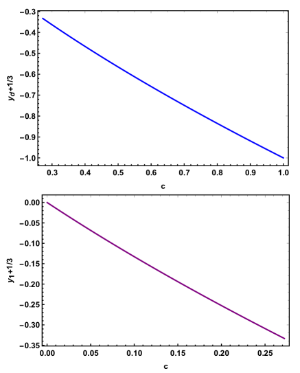
Figure 1: The functions $z_{d}=y_{d}+1/3$ and $z_{1}=y_{1}+1/3$. The upper panel corresponds to the real root of the cubic equation for $K<c^{2}<1$. The lower panel corresponds to the root $y_{1}$ when $0<c^{2}<K$. They are both monotonic decreasing functions of $c$ and remain negative. Thus, these solutions do not give light rings.

Next, we turn to the case $c\neq 0$. To solve Eq. (3.8), we let

$$y=z-q/3>-q/3\,.$$ (3.9)

In the following, for simplicity but without loss of generality, we set $q=1$. Then Eq. (3.8) becomes

$$y^{3}-\frac{1}{3}y+2c^{2}-\frac{2}{27}=0\,.$$ (3.10)

In order to find the roots of the cubic equation, it’s covenient to define

$$u=-\frac{1}{3}\,,\quad v=2c^{2}-\frac{2}{27}\,,\quad\text{and}\quad\Delta=\mathopen{}\mathclose{{}\left(\frac{v}{2}}\right)^{2}+\mathopen{}\mathclose{{}\left(\frac{u}{3}}\right)^{3}=c^{2}\mathopen{}\mathclose{{}\left(c^{2}-\frac{2}{27}}\right)\,.$$ (3.11)

Then, from $\Delta=0$, we can identify a critical constant $K\equiv\frac{2}{27}$. And, when $c^{2}>K$, Eq. (3.10) has only one real root taking in this form

$$y_{d}=\frac{-1-\sqrt{3}i+i(i+\sqrt{3})\mathopen{}\mathclose{{}\left(1-27c^{2}+3\sqrt{-6c^{2}+81c^{4}}}\right)^{2/3}}{6\mathopen{}\mathclose{{}\left(1-27c^{2}+3\sqrt{-6c^{2}+81c^{4}}}\right)^{1/3}}\,.$$ (3.12)

where $i$ is the imaginary unit. One can then easily check that $y_{d}+1/3<0$ is always true for $c^{2}>K$ which does not satisfy Eq. (3.9) (see the upper panel in Fig. 1), meaning there is no light ring.

Next, we consider the case $\Delta=0$, that is, $c^{2}=K$. We find the roots of the cubic equation read

$$y_{m1}=y_{m2}=1/3\quad\text{and}\quad y_{m3}=-2/3\,.$$ (3.13)

Obviously, $y_{m3}$ should be dropped and we find there are two degenerate light rings.

Now, let us turn to the case $\Delta<0$, that is $c^{2}<K$. We have three different real roots,

$$y_{w} = \frac{2}{3}\cos\frac{\Theta+2w\pi}{3}$$ (3.14)

where $w=-1,0,1$ and

$$\Theta=\arccos(1-27c^{2}).$$ (3.15)

From the lower panel of Fig. 1, we can see $(y_{1}+1/3)^{2}-c^{2}<0$ for $0<c^{2}<K$ and thus $y_{1}$ should be excluded. The other two LRs occur at

$$r_{1} = \sqrt{z_{0}^{2}-c^{2}}\mathopen{}\mathclose{{}\left(1+\frac{1}{z_{0}}}\right)\,,$$ (3.16)

$$r_{2} = \sqrt{z_{-1}^{2}-c^{2}}\mathopen{}\mathclose{{}\left(1+\frac{1}{z_{-1}}}\right)\,,$$ (3.17)

where

$$z_{w}=\frac{1}{3}\mathopen{}\mathclose{{}\left(1+2\cos\frac{\Theta+2w\pi}{3}}\right)\,.$$ (3.18)

with $w=-1,0$. One can check that and the outer LR ($r=r_{1}$) is unstable and the inner LR ($r=r_{2}$) is stable. This is consistent to the general conclusion for UCOs[25, 29].

Now we pay special attention to the regime $c\to 0$, i.e., the black hole limit. We can expand the roots to the order of $c^{2}$ and find

$$R_{0} = 1-\frac{5}{2}c^{2},$$ (3.19)

$$R_{-1} = c\,,$$ (3.20)

which correspond to

$$r_{0} = 2q-3\frac{c^{2}}{q}\,,$$ (3.21)

$$r_{-1} = \frac{q}{\sqrt{2}}+\frac{3}{2}c-\frac{9c^{2}}{4\sqrt{2}q}\,,$$ (3.22)

where we have put the charge $q$ back to the formula. We see that as $c\to 0$, $r_{0}\to 2q$ which just reduces to the light ring of the extremal RN black hole. However, as $c\to 0$, $r_{-1}\to q/\sqrt{2}$. This result does approach the RN limit $c=0$, where such a light ring does not exist. To understand this apparent inconsistency, we notice that Eq. (3.22) is obtained by substituting Eq. (3.20) into Eq. (2.9) and then taking the limit $c\to 0$. For the extremal RN solution, we let $c=0$ in Eq. (2.9) and then taking the limit $R\to 0$. This lead to $r=q$, which is not a LR as we have discussed.

4 Long-lived QNM modes of a quasi-black hole spacetime

In section 3, we have found when $0<c^{2}<K$, the quasi-black hole can be seen as an UCO with an inner stable light ring and an outer unstable light ring. In this section, we are going to verify whether QBHs have stability problem under linear gravitational perturbations. More precisely, we would calculate the frequencies of QNMs to see if there are long-lived modes in the parameter range where the LRs exist. Considering that QNMs have been studied widely in the standard coordinates $(t,r,\theta,\phi)$, our strategy for dealing with the QNMs is that we first obtain the QNM equations in the coordinates $(t,r,\theta,\phi)$ based on a general formula for any spherically symmetric metric in [24], and then we transform the equations into a form of the coordinate $R$ since it’s more convenient to use $R$ for the calculations about QBHs as we have done in section 3. Now, let us rewrite the spherically symmetric metric in the form

$$ds^{2}=-B(r)dt^{2}+A(r)dr^{2}+r^{2}(d\theta^{2}+\sin^{2}\theta d\phi^{2})$$ (4.1)

It is not difficult to find that the two metric components in Eqs. (4.1) and (2.5) are related by

$$B = \frac{1}{U^{2}}=\frac{z^{2}}{(z+q)^{2}}\,,$$ (4.2)

$$\frac{1}{\sqrt{A}} \equiv \frac{1}{W}=1+\frac{R}{U}\frac{dU}{dR}=\frac{z^{2}(q+z)}{z^{2}(q+z)-qR^{2}}\,.$$ (4.3)

To calculate the quasi-normal modes, we start with the master equation[24]

$$\mathopen{}\mathclose{{}\left[\frac{\partial^{2}}{\partial_{t}^{2}}-\frac{\partial^{2}}{\partial_{r_{\ast}}^{2}}+V_{sl}(r)}\right]\Psi(r,t)=0\,,$$ (4.4)

which can describe perturbations of different fields in the background of the metric (4.1). In the potential $V_{sl}(r)$, when $l\geq s$, $s=0,1,2$ correspond to the perturbations of massless scalar fields, Maxwell fields and a generically anisotropic fluid, respectively. The tortoise coordinate $r_{\ast}$ is defined by $dr/dr_{\ast}=\sqrt{B/A}$, and the potential $V_{sl}(r)$ takes the form

$$V_{sl}(r)=B\mathopen{}\mathclose{{}\left[\frac{l(l+1)}{r^{2}}+\frac{1-s^{2}}{2rA}\mathopen{}\mathclose{{}\left(\frac{B^{\prime}}{B}-\frac{A^{\prime}}{A}}\right)+8\pi(p_{\text{rad}}-\rho)\delta_{s2})}\right]\,.$$ (4.5)

Alternatively, from the relationship between $r$ and $R$, that is $r=RU$, $V_{sl}(r)$ can be reexpressed in the coordinate $R$ as

$$\bar{V}_{sl}(R)\equiv V_{sl}(r)=\frac{1}{U^{2}}\mathopen{}\mathclose{{}\left[\frac{l(l+1)}{R^{2}U^{2}}-\frac{1-s^{2}}{RUW^{2}}\frac{d}{dR}\mathopen{}\mathclose{{}\left(\log U+\log W}\right)\frac{dR}{dr}+8\pi(p_{\text{rad}}-\rho)\delta_{s2}}\right].$$ (4.6)

where $W\equiv\sqrt{A}$ is introduced in Eq. (4.3) And the the radial pressure $p_{\text{rad}}$ and the energy density $\rho$ of the QBH are needed to be introduced and we find they have the following expressions

$$p_{\text{rad}}=T^{r}_{r}=-\frac{q^{2}R^{2}}{8\pi z^{2}(q+z)^{4}}\quad\text{and}\quad\rho=-T^{t}_{t}=\frac{q[qR^{2}+6c^{2}(1+z)]}{8\pi z^{2}(q+z)^{4}}\,,$$ (4.7)

By the way, we want to stress that by calculating

$$p_{\text{rad}}+\rho=\frac{3c^{2}(1+z)}{4\pi z^{2}(1+z)^{4}}>0\,,$$ (4.8)

we can confirm that the weak energy condition always holds for the QBH. Next, assuming a time dependence $\Psi(r,t)=\psi(r)e^{-i\omega t}$, from the Eq. (4.4) we can see that the radial function $\psi(r)$ satisfies a Schr$\ddot{\text{o}}$dinger-like equation

$$\frac{d^{2}\psi}{dr_{\ast}^{2}}+[\omega^{2}-V_{sl}(r)]\psi=0,$$ (4.9)

with

$$r_{\ast}=\int_{0}^{R}UR\frac{dr}{dR}dR=R+\frac{\arctan(R/c)}{c}+2\operatorname{arctanh}\frac{R}{\sqrt{c^{2}+R^{2}}}\,.$$ (4.10)

Alternatively, we have

$$\frac{(c^{2}+R^{2})^{2}}{(1+\sqrt{c^{2}+R^{2}})^{4}}\bar{\psi}^{\prime\prime}(R)+\frac{2R(c^{2}+R^{2})}{(1+\sqrt{c^{2}+R^{2}})^{5}}\bar{\psi}^{\prime}(R)+[\omega^{2}-\bar{V}_{sl}(R)]\bar{\psi}(R)=0\,,$$ (4.11)

where we have used $\bar{\psi}(R)\equiv\psi(r)$.

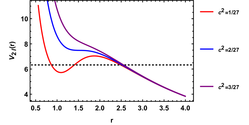
Figure 2: The variations of the effective potential function $V_{2l}$ with respect to $r$ for $c^{2}=1/27,2/27,3/27$, respectively. Here we choose $l=10\gg 1$.

Figure 3: A diagram of the potential function $V_{2l}$ with respect to $r$ for $0<c^{2}<2/27$.

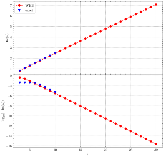
Figure 4: Real and imaginary parts of the QNMs of the QBH with $c^{2}=1/27$. The red lines are the WKB results and the blue inverted triangles reveal the numerical results obtained from the direct integration method. From the lower panel, we can see that QNMs are indeed long-lived modes, which indicates a possible nonlinear instability of the spacetime.

In this article, we focus on gravitational perturbations, that is, $s=2$. Thus at the center of the quasi-black hole, $R\to 0$, we find

$$r_{\ast}\to\frac{(\sqrt{c^{2}}+1)^{2}}{c^{2}}R\to 0,\quad\bar{V}_{2l}\to\frac{c^{4}l(l+1)}{(1+\sqrt{c^{2}})^{4}R^{2}}=\frac{l(l+1)}{r_{\ast}^{2}}\,,$$ (4.12)

and at infinity, $R\to\infty$, we have

$$r_{\ast}\to R,\quad\bar{V}_{2l}\to\frac{l(l+1)}{R^{2}}=\frac{l(l+1)}{r_{\ast}}\,.$$ (4.13)

Furthermore, we have at the center

$$R\to 0,\quad\bar{\psi}\sim C_{1}R^{l+1}+C_{2}R^{-l}\,,$$ (4.14)

and at infinity

$$R\to\infty,\quad\bar{\psi}\sim D_{1}e^{-i\omega R}+D_{2}e^{i\omega R}\,.$$ (4.15)

Regular gravitational perturbations should have $C_{2}=0$ at the center, and at infinity, the gravitational perturbations should be outgoing, that is, $D_{1}=0$. In the following, we shall determine the values of $\omega$ in terms of the coordinate $R$. We rewrite $\bar{\psi}(R)$ in this form

$$\bar{\psi}(R)=R^{l+1}e^{i\omega R}\chi(R)$$ (4.16)

This asymptotic solution corresponds to an outgoing boundary condition at infinity and a regular boundary condition near the center of the quasi-black black. The frequencies of the perturbations can be seen as compositions of quasinormal modes . With the specific boundary conditions (4.14) and (4.15), the radial equation (4.11) can be solved as an eigenvalue problem. Note that only some discrete eigenfrequencies $\omega$ can satisfy both the radial equation and boundary conditions. Since the frequency $\omega$ would be a complex number in general, one can always write the eigenfrequency as the form $\omega=\omega_{R}+i\omega_{I}$. As we assume $\Psi(r,t)=\psi(r)e^{-i\omega t}$, the amplitude of perturbation will grow exponentially when the imaginary part $\omega_{I}>0$, which implies that the black hole is unstable at least at the linear perturbation level. Then in principle, we can identify the eigenvalues of $\omega$ by solving this equation for any $l\geq s$ numerically.

In practice, the behaviors of $\omega$ are very sensitive to the effective potential $V_{2l}$. In particular, we are interested in the eikonal regime, that is, $l\gg 1$. In Fig. 2, we show examples of the effective potential $V_{2l}$ at $l=10$. Obviously, we can see that at $c^{2}=1/27$, the effective potential $V_{2l}$ has a local maximun and a local minimum, while for $c^{2}=3/27$, the effective potential $V_{2l}$ only has a local maximun. At $c^{2}=2/27$, the effective potential has a degenerate extreme point. It has been argued in [24, 51] that long-lived modes may be possible in the eikonal limit, that is, for $l\gg 1$, compared to the usual modes, there may be some long-lived modes whose damping time grows exponentially with $l$, when the potential necessarily has a local minimum. In addition, from Eq. (4.5) we observe that when $l\gg\frac{r}{2A}\mathopen{}\mathclose{{}\left(\frac{B^{\prime}}{B}-\frac{A^{\prime}}{A}}\right)$ and $l\gg 8\pi r^{2}(p_{\text{rad}}-\rho)$, the effective potential $V_{sl}\simeq\frac{l^{2}}{r^{2}U^{2}}$, which has the same expression as the effective potential $V=\frac{L^{2}}{R^{2}U^{4}}$ for null geodesics (see Eq. (3.6))if we identify $l$ with $L$. Noting that for asymptotic spacetimes, we have $\frac{r}{2A}\mathopen{}\mathclose{{}\left(\frac{B^{\prime}}{B}-\frac{A^{\prime}}{A}}\right)\sim\frac{1}{r^{m}}$ with $m\geq 1$ and $8\pi r^{2}(p_{\text{rad}}-\rho)\sim\frac{1}{r^{2}}$ when $r\to\infty$. Thus, as long as $l$ is big enough, we always have $V_{2l}\approx V$. In section 3, we have found that $c^{2}=K$ is a critical point for the effective potential of null geodescis. For $c^{2}<K$, the effective potential $V$ has a local minimum, corresponding to a stable LR. So for gravitational perturbations, the effective potential $V_{2l}$ also has a local minimun when $l$ is large enough in the eikonal regime. Therefore, we can infer that when $c^{2}<K$, i.e., a stable LR exists in the QBH spacetime, it becomes possible that the spectrum of linear QNMs contains the long-lived modes. Next, we are going to verify this relation by calculating the values of $\omega$.

Following standard numerical methods, we would use the method of direct integration to obtain the values of $\omega$. On the other hand, as shown in [59, 60, 24], when the potential $V_{2l}$ has a local maximum and a local minimum (see Fig. 3), for $l\gg 1$, the real part of the frequency $\omega_{R}$ in four spacetime dimensions is given by the WKB approximation

$$\int_{r_{a}}^{r_{b}}\frac{dr}{\sqrt{B/A}}\sqrt{\omega_{R}^{2}-V_{2l}(r)}=\pi(n+1/2)=\int_{R_{a}}^{R_{b}}dRU(R)W(R)\sqrt{\omega_{R}^{2}-\bar{V}_{2l}(R)}\frac{dr}{dR}$$ (4.17)

where $n$ is a positive integer and $r_{a}$ and $r_{b}$ are two smaller roots of the equation $\omega_{R}^{2}-V_{sl}=0$ (see Fig. 3). Obviously, we can easily conclude $\omega_{R}\in(V_{2l}^{min},V_{2l}^{max})$. In addition, $R_{a}$ and $R_{b}$ are the roots corresponding to $r_{a}$ and $r_{b}$ in the $R$ coordinate, that is, $r_{a,b}=R_{a,b}U(R_{a,b})$. In addition, the imaginary part of the frequency $\omega_{I}$ is given by

$$\omega_{I}=-\frac{1}{8\omega_{R}\gamma}e^{-\Gamma}\,,$$ (4.18)

with

$$\Gamma = 2\int_{r_{b}}^{r_{c}}\frac{dr}{\sqrt{B/A}}\sqrt{V_{sl}(r)-\omega_{R}^{2}}=\int_{R_{b}}^{R_{c}}dRU(R)W(R)\sqrt{\bar{V}_{2l}(R)-\omega_{R}^{2}}\frac{dr}{dR}$$ (4.19)

$$\gamma = \int_{r_{a}}^{r_{b}}\frac{dr}{\sqrt{B/A}}\frac{\cos^{2}\chi(r)}{\sqrt{\omega_{R}^{2}-V_{sl}(r)}}=\int_{R_{a}}^{R_{b}}dR\frac{U(R)W(R)\cos^{2}\bar{\chi}(R)}{\sqrt{\omega_{R}^{2}-\bar{V}_{2l}(r)}}\frac{dr}{dR}$$ (4.20)

$$\chi(r) = -\frac{\pi}{4}+\int_{r}^{r_{b}}\frac{dr}{\sqrt{B/A}}\sqrt{\omega_{R}^{2}-V_{2l}(r)}$$ (4.21)

$$= \bar{\chi}(R)=-\frac{\pi}{4}+\int_{R}^{R_{a}}dRU(R)W(R)\sqrt{\omega_{R}^{2}-\bar{V}_{2l}(R)}\frac{dr}{dR}\,,$$

where $r_{c}=R_{c}U(R_{c})$ is the largest root of the equation $\omega_{R}^{2}-V_{sl}=0$. We show the values of $\omega$ in Fig. 4 from both the numerical integration and WKB method. From the figure, we can see that the results given by the two methods agree very well. Furthermore, the imaginary parts of the results show that the QNMs are indeed long-lived modes.

On the other hand, we would like to give some comments on the case $c^{2}\geq K$, in which there have been found no stable LRs in section 3. As shown in the Fig. 2, the effective potential $V_{2l}$ would have no local maximum in the eikonal limit. Following the similar analysis for planar AdS black holes in [59], one can see that there are no long-lived modes survived in the linear perturbations of gravitations when $c^{2}\geq K$, that is, there are no stable LRs.

5 Conclusion

We have revisited the quasi-black hole spacetimes. In the parameter range $0<c^{2}<2/27$, we have found two LRs of which the inner one is stable and the outer one is unstable. They disappear altogether for $c^{2}>2/27$ with the critical value $c^{2}=2/27$ corresponding to a degenerate LR. It’s worth noting that near the black hole limit, i.e., $c\to 0$, we found there always exists a stable inner LR while it has no correspondence in the black hole solution (when $c$ is strictly zero). We have also calculated the quasinormal modes of the QBHs. The WKB method and numerical method both suggest that long-live modes survive when light rings exist, indicating that quasi-black hole spacetimes containing LRs, as a kind of ultracompact objects, may not be stable. Compared to the previous results on ultracompact stars that the exteriors are Schwarzschild solutions, the LRs in the QBH model can turn on smoothly at a critical value of $c$. Therefore, from another perspective, our work provides a concrete example to support the conjecture that observation of light rings may be strong evidence for black holes.

The quasi-black hole model indicates that LRs could be a signature exclusive for black holes. However, a quasi-black hole cannot be treated as a real astrophysical body, since it has the total charge $q$ equal to the mass $M$, while in astrophysically reasonable situations, the charge is usually much smaller than the mass [61]. Thus, future studies shall focus on more realistic objects. For example, it would be important to consider UCO models with rotation since astrophysical bodies with high spin-mass ratio have been observed.

References

- [1] S. K., “ber das Gravitationsfeld eines Massenpunktes nach der Einstein’schen Theorie,” Sitzungsberichte der Deutschen Akademie der Wissenschaften zu Berlin, Klasse fr Mathematik, Physik, und Technik 189 (1916) .
- [2] LIGO Scientific, Virgo Collaboration, B. P. Abbott et al., “Observation of Gravitational Waves from a Binary Black Hole Merger,” Phys. Rev. Lett. 116 no. 6, (2016) 061102, arXiv:1602.03837 [gr-qc].
- [3] LIGO Scientific, Virgo Collaboration, B. P. Abbott et al., “GW151226: Observation of Gravitational Waves from a 22-Solar-Mass Binary Black Hole Coalescence,” Phys. Rev. Lett. 116 no. 24, (2016) 241103, arXiv:1606.04855 [gr-qc].
- [4] LIGO Scientific, Virgo Collaboration, B. P. Abbott et al., “GW170817: Observation of Gravitational Waves from a Binary Neutron Star Inspiral,” Phys. Rev. Lett. 119 no. 16, (2017) 161101, arXiv:1710.05832 [gr-qc].
- [5] Event Horizon Telescope Collaboration, K. Akiyama et al., “First M87 Event Horizon Telescope Results. I. The Shadow of the Supermassive Black Hole,” Astrophys. J. Lett. 875 (2019) L1, arXiv:1906.11238 [astro-ph.GA].
- [6] Event Horizon Telescope Collaboration, K. Akiyama et al., “First M87 Event Horizon Telescope Results. II. Array and Instrumentation,” Astrophys. J. Lett. 875 no. 1, (2019) L2, arXiv:1906.11239 [astro-ph.IM].
- [7] Event Horizon Telescope Collaboration, K. Akiyama et al., “First M87 Event Horizon Telescope Results. III. Data Processing and Calibration,” Astrophys. J. Lett. 875 no. 1, (2019) L3, arXiv:1906.11240 [astro-ph.GA].
- [8] Event Horizon Telescope Collaboration, K. Akiyama et al., “First M87 Event Horizon Telescope Results. VII. Polarization of the Ring,” Astrophys. J. Lett. 910 no. 1, (2021) L12, arXiv:2105.01169 [astro-ph.HE].
- [9] Event Horizon Telescope Collaboration, K. Akiyama et al., “First M87 Event Horizon Telescope Results. VIII. Magnetic Field Structure near The Event Horizon,” Astrophys. J. Lett. 910 no. 1, (2021) L13, arXiv:2105.01173 [astro-ph.HE].
- [10] I. Banerjee, S. Chakraborty, and S. SenGupta, “Silhouette of M87*: A New Window to Peek into the World of Hidden Dimensions,” Phys. Rev. D 101 no. 4, (2020) 041301, arXiv:1909.09385 [gr-qc].
- [11] Y. Hou, M. Guo, and B. Chen, “Revisiting the shadow of braneworld black holes,” Phys. Rev. D 104 no. 2, (2021) 024001, arXiv:2103.04369 [gr-qc].
- [12] R. Kumar and S. G. Ghosh, “Black Hole Parameter Estimation from Its Shadow,” Astrophys. J. 892 (2020) 78, arXiv:1811.01260 [gr-qc].
- [13] Z. Hu, Z. Zhong, P.-C. Li, M. Guo, and B. Chen, “QED effect on a black hole shadow,” Phys. Rev. D 103 no. 4, (2021) 044057, arXiv:2012.07022 [gr-qc].
- [14] Z. Zhong, Z. Hu, H. Yan, M. Guo, and B. Chen, “QED Effects on Kerr Black Hole Shadows immersed in uniform magnetic fields,” arXiv:2108.06140 [gr-qc].
- [15] H.-M. Wang, Y.-M. Xu, and S.-W. Wei, “Shadows of Kerr-like black holes in a modified gravity theory,” JCAP 03 (2019) 046, arXiv:1810.12767 [gr-qc].
- [16] P.-C. Li, M. Guo, and B. Chen, “Shadow of a Spinning Black Hole in an Expanding Universe,” Phys. Rev. D 101 no. 8, (2020) 084041, arXiv:2001.04231 [gr-qc].
- [17] Q. Gan, P. Wang, H. Wu, and H. Yang, “Photon ring and observational appearance of a hairy black hole,” Phys. Rev. D 104 no. 4, (2021) 044049, arXiv:2105.11770 [gr-qc].
- [18] M. Wang, S. Chen, and J. Jing, “Kerr Black hole shadows in Melvin magnetic field with stable photon orbits,” arXiv:2104.12304 [gr-qc].
- [19] X.-X. Zeng, G.-P. Li, and K.-J. He, “The shadows and observational appearance of a noncommutative black hole surrounded by various profiles of accretions,” arXiv:2106.14478 [hep-th].
- [20] M. Guo, S. Song, and H. Yan, “Observational signature of a near-extremal Kerr-Sen black hole in the heterotic string theory,” Phys. Rev. D 101 no. 2, (2020) 024055, arXiv:1911.04796 [gr-qc].
- [21] H. Yan, “Influence of a plasma on the observational signature of a high-spin Kerr black hole,” Phys. Rev. D 99 no. 8, (2019) 084050, arXiv:1903.04382 [gr-qc].
- [22] M. Guo, N. A. Obers, and H. Yan, “Observational signatures of near-extremal Kerr-like black holes in a modified gravity theory at the Event Horizon Telescope,” Phys. Rev. D 98 no. 8, (2018) 084063, arXiv:1806.05249 [gr-qc].
- [23] A. F. Zakharov, F. De Paolis, G. Ingrosso, and A. A. Nucita, “Shadows as a tool to evaluate black hole parameters and a dimension of spacetime,” New Astron. Rev. 56 (2012) 64–73.
- [24] V. Cardoso, L. C. B. Crispino, C. F. B. Macedo, H. Okawa, and P. Pani, “Light rings as observational evidence for event horizons: long-lived modes, ergoregions and nonlinear instabilities of ultracompact objects,” Phys. Rev. D 90 no. 4, (2014) 044069, arXiv:1406.5510 [gr-qc].
- [25] M. Guo and S. Gao, “Universal Properties of Light Rings for Stationary Axisymmetric Spacetimes,” Phys. Rev. D 103 no. 10, (2021) 104031, arXiv:2011.02211 [gr-qc].
- [26] P. V. P. Cunha and C. A. R. Herdeiro, “Stationary black holes and light rings,” Phys. Rev. Lett. 124 no. 18, (2020) 181101, arXiv:2003.06445 [gr-qc].
- [27] R. Ghosh and S. Sarkar, “Light rings of stationary spacetimes,” Phys. Rev. D 104 no. 4, (2021) 044019, arXiv:2107.07370 [gr-qc].
- [28] S. Hod, “On the number of light rings in curved spacetimes of ultra-compact objects,” Phys. Lett. B 776 (2018) 1–4, arXiv:1710.00836 [gr-qc].
- [29] P. V. P. Cunha, E. Berti, and C. A. R. Herdeiro, “Light-Ring Stability for Ultracompact Objects,” Phys. Rev. Lett. 119 no. 25, (2017) 251102, arXiv:1708.04211 [gr-qc].
- [30] C. A. R. Herdeiro, A. M. Pombo, E. Radu, P. V. P. Cunha, and N. Sanchis-Gual, “The imitation game: Proca stars that can mimic the Schwarzschild shadow,” JCAP 04 (2021) 051, arXiv:2102.01703 [gr-qc].
- [31] X. Wang, P.-C. Li, C.-Y. Zhang, and M. Guo, “Novel shadows from the asymmetric thin-shell wormhole,” Phys. Lett. B 811 (2020) 135930, arXiv:2007.03327 [gr-qc].
- [32] J. Peng, M. Guo, and X.-H. Feng, “Observational Signature and Additional Photon Rings of Asymmetric Thin-shell Wormhole,” arXiv:2102.05488 [gr-qc].
- [33] R. Brito, V. Cardoso, and H. Okawa, “Accretion of dark matter by stars,” Phys. Rev. Lett. 115 no. 11, (2015) 111301, arXiv:1508.04773 [gr-qc].
- [34] G. Narain, J. Schaffner-Bielich, and I. N. Mishustin, “Compact stars made of fermionic dark matter,” Phys. Rev. D 74 (2006) 063003, arXiv:astro-ph/0605724.
- [35] M. Raidal, S. Solodukhin, V. Vaskonen, and H. Veermäe, “Light Primordial Exotic Compact Objects as All Dark Matter,” Phys. Rev. D 97 no. 12, (2018) 123520, arXiv:1802.07728 [astro-ph.CO].
- [36] V. Cardoso and P. Pani, “Testing the nature of dark compact objects: a status report,” Living Rev. Rel. 22 no. 1, (2019) 4, arXiv:1904.05363 [gr-qc].
- [37] P. V. P. Cunha, C. A. R. Herdeiro, and M. J. Rodriguez, “Does the black hole shadow probe the event horizon geometry?,” Phys. Rev. D 97 no. 8, (2018) 084020, arXiv:1802.02675 [gr-qc].
- [38] H. C. D. Lima, Junior., L. C. B. Crispino, P. V. P. Cunha, and C. A. R. Herdeiro, “Can different black holes cast the same shadow?,” Phys. Rev. D 103 no. 8, (2021) 084040, arXiv:2102.07034 [gr-qc].
- [39] M. Zhang and M. Guo, “Can shadows reflect phase structures of black holes?,” Eur. Phys. J. C 80 no. 8, (2020) 790, arXiv:1909.07033 [gr-qc].
- [40] M. S. Morris, K. S. Thorne, and U. Yurtsever, “Wormholes, Time Machines, and the Weak Energy Condition,” Phys. Rev. Lett. 61 (1988) 1446–1449.
- [41] M. Visser, “Traversable wormholes: Some simple examples,” Phys. Rev. D 39 (1989) 3182–3184, arXiv:0809.0907 [gr-qc].
- [42] E. Poisson and M. Visser, “Thin shell wormholes: Linearization stability,” Phys. Rev. D 52 (1995) 7318–7321, arXiv:gr-qc/9506083.
- [43] X. Wang and S. Gao, “Static spherically symmetric thin shell wormhole colliding with a spherical thin shell,” Phys. Rev. D 93 no. 6, (2016) 064027, arXiv:1511.05420 [gr-qc].
- [44] E. Seidel and W.-M. Suen, “Formation of solitonic stars through gravitational cooling,” Phys. Rev. Lett. 72 (1994) 2516–2519, arXiv:gr-qc/9309015.
- [45] R. Brito, V. Cardoso, C. A. R. Herdeiro, and E. Radu, “Proca stars: Gravitating Bose–Einstein condensates of massive spin 1 particles,” Phys. Lett. B 752 (2016) 291–295, arXiv:1508.05395 [gr-qc].
- [46] F. Di Giovanni, N. Sanchis-Gual, C. A. R. Herdeiro, and J. A. Font, “Dynamical formation of Proca stars and quasistationary solitonic objects,” Phys. Rev. D 98 no. 6, (2018) 064044, arXiv:1803.04802 [gr-qc].
- [47] J. L. Friedman, “Ergosphere instability,” Communications in Mathematical Physics 63 (1978) 243-C255.
- [48] C. B. M. H. Chirenti and L. Rezzolla, “On the ergoregion instability in rotating gravastars,” Phys. Rev. D 78 (2008) 084011, arXiv:0808.4080 [gr-qc].
- [49] P. Pani, V. Cardoso, M. Cadoni, and M. Cavaglia, “Ergoregion instability of black hole mimickers,” PoS BHGRS (2008) 027, arXiv:0901.0850 [gr-qc].
- [50] P. Pani, E. Barausse, E. Berti, and V. Cardoso, “Gravitational instabilities of superspinars,” Phys. Rev. D 82 (2010) 044009, arXiv:1006.1863 [gr-qc].
- [51] J. Keir, “Slowly decaying waves on spherically symmetric spacetimes and ultracompact neutron stars,” Class. Quant. Grav. 33 no. 13, (2016) 135009, arXiv:1404.7036 [gr-qc].
- [52] J. P. S. Lemos and O. B. Zaslavskii, “Black hole mimickers: Regular versus singular behavior,” Phys. Rev. D 78 (2008) 024040, arXiv:0806.0845 [gr-qc].
- [53] A. Lue and E. J. Weinberg, “Gravitational properties of monopole space-times near the black hole threshold,” Phys. Rev. D 61 (2000) 124003, arXiv:hep-th/0001140.
- [54] A. Lue and E. J. Weinberg, “Monopoles and the emergence of black hole entropy,” Gen. Rel. Grav. 32 (2000) 2113–2118, arXiv:gr-qc/0004001.
- [55] J. P. S. Lemos and E. J. Weinberg, “Quasiblack holes from extremal charged dust,” Phys. Rev. D 69 (2004) 104004, arXiv:gr-qc/0311051.
- [56] J. P. S. Lemos and O. B. Zaslavskii, “Quasi black holes: Definition and general properties,” Phys. Rev. D 76 (2007) 084030, arXiv:0707.1094 [gr-qc].
- [57] J. P. S. Lemos and O. B. Zaslavskii, “Entropy of quasiblack holes,” Phys. Rev. D 81 (2010) 064012, arXiv:0904.1741 [gr-qc].
- [58] J. P. S. Lemos and V. T. Zanchin, “Quasiblack holes with pressure: relativistic charged spheres as the frozen stars,” Phys. Rev. D 81 (2010) 124016, arXiv:1004.3574 [gr-qc].
- [59] G. Festuccia and H. Liu, “A Bohr-Sommerfeld quantization formula for quasinormal frequencies of AdS black holes,” Adv. Sci. Lett. 2 (2009) 221–235, arXiv:0811.1033 [gr-qc].
- [60] S. A. Gurvitz, “Novel approach to tunneling problems,” Phys. Rev. A 38 (1988) 1747–1759.
- [61] R. M. Wald, General Relativity (University of Chicago, Chicago, 1984).