Sparse Array Capon Beamformer Design Availing Deep Learning

Abstract

The paper considers sparse array design for receive beamforming achieving maximum signal-to-interference plus noise ratio (MaxSINR). We develop a design approach based on supervised neural network where class labels are generated using an efficient sparse beamformer spectral analysis (SBSA) approach. SBSA uses explicit information of the unknown narrowband interference environment for training the network and bears close performance to training using enumerations, i.e., exhaustive search which is computationally prohibitive for large arrays. The employed DNN effectively approximates the unknown mapping from the input received data spatial correlations to the output of sparse configuration with effective interference mitigation capability. The problem is posed as a multi-label classification problem where the selected antenna locations achieving MaxSINR are indicated by the output layer of DNN. In addition to evaluating the performance of the DNN in terms of the classification accuracy, we evaluate the performance in terms of the the ability of the classified sparse array to mitigate interference and maximize signal power. It is shown that even in the case of miss-classification, where at least one sensor location doesn’t match the optimal locations, the DNN effectively learns the sub-optimal sparse configuration which has desirable SINR characteristics. This shows the ability of the DNN to learn the proposed optimization algorithms, hence paving the way for efficient real-time implementation.

I Introduction

Sparse array design reduces system transceiver costs by reducing the hardware and processing complexity through sensor selection. It is useful in multitude of sensor signal processing tasks in MIMO communications, radar/sonar, satellite navigation, radio telescopes, speech enhancement and medical imaging applications [1, 2, 3, 4, 5, 6]. The performance gains in using sparse arrays stem from their inherent ability of tending the additional degrees of freedom to accomplish pre-defined metrics. Several different performance metrics have been proposed in the literature, and can generally be categorized into environment-independent or environment-dependent design [7, 8]. The latter requires array reconfigurability since, the receiver performance then largely depends on the operating environment, which may change according to the source and interference signals and locations. This is in contrast to environment-independent sparse arrays whose configurations follow certain formulas and seek to attain structured sparse configurations with extended aperture co-arrays. The driving objective, in this case, is to enable direction of arrival (DOA) estimation of more sources than the available physical sensors. Common examples of structured sparse arrays are the nested and coprime arrays [9, 10, 11].

Reliably extracting a desired signal waveform by enhancing SINR has a direct bearing on improving target detection and localization for radar signal processing, increasing throughput or channel capacity for MIMO wireless communication systems, and enhancing resolution capability in medical imaging [12, 13, 14]. Maximizing signal-to-noise ratio (MaxSNR) and MaxSINR criteria have been shown to yield significantly efficient beamforming performance and interference mitigation. For sparse array design, the MaxSINR beamforming performance depends mainly on the selected positions of the sensors as well as the locations of the desired source and interferers in the field of view (FOV) [15, 16, 17, 18, 19, 20]. It is noted that with sparse arrays, Capon beamforming must not only find the optimum weights, as commonly used in uniform arrays, but also the optimum array configuration [14]. This is clearly an entwined optimization problem and requires attaining maximum SINR considering all possible sparse array configurations.

Sparse array design typically involves the selection of a subset of uniform grid points for sensor placements. For a given number of sensors, it is assumed that the number of perspective grid points, spaced by half wavelength, is limited due to a size constraint on the physical aperture. For environment-dependent sparse arrays, the antenna positions are selected from uniformly spaced locations that are served by a limited number of transceiver chains. These antenna positions would vary with the changing environment. Rapid array reconfigurability has been made possible by advances in efficient sensor switching technologies that readily activates a subset of sensors on a predefined grid points. The system cost can then be significantly reduced by limiting the number of expensive transceivers chains at any given time [21, 22, 23, 24].

Environment-dependent sparse array design algorithms generally follow two different approaches. The designs based on prior knowledge of interference parameters, essentially require that the real time interference parameters, such as DOAs and respective SINRs, are either known or estimated apriori in real time. The other approach is more practical as it doesn’t require the information of interfering environment which is the case in Capon beamforming. In both cases, several iterative algorithms have been proposed to optimize the sparse array beamformer design. Although, convex based optimization algorithms, such as semidefinite relaxation (SDR) and successive convex approximation (SCA) have been developed to yield sparse configurations with desirable beamforming performances [19, 20], real time implementations of these algorithms remain limited due to the relatively high computation cost. The problem becomes more pronounced in rapidly changing environments which result from temporal and spatial non-stationary behaviors of the sources in the field of view.

In this paper, we propose a sparse beamformer methodology implementing data-driven array design by training the DNN to learn and mimic the sparse beamforming design algorithms. DNNs have shown great potential due to their demonstrated ability of feature learning in many applications, including computer vision, speech recognition, and natural language processing [25, 26, 27]. In the underlying problem, DNN is used to approximate the unknown mapping from the receiver data spatial correlations to the output array configuration. It is shown that DNN effectively learns the optimum array structure which makes DNN, in requiring a few simple operations, suitable for real-time implementation.

Towards DNN-based sparse array design, the training data may follow two different approaches. In the first approach, we use enumeration technique to generate the training labels for any given sensor correlation function. In this case, MaxSINR array configuration is obtained by sifting through all possible sparse configurations and choosing the best performing array topology. Although the training data is generated offline, it becomes infeasible to obtain an optimum configuration even for a moderate size arrays due to the enormous number of sensor permutations. In order to circumvent this problem, we propose the second approach that expedites the generation of a large number of training data labels to input the DNN. For any specific environment presented in the training set, the proposed approach considers the corresponding array spatial spectrum and incorporates the sensor correlation lag redundancy for determining the desired array structure.

Recently, ‘learn to optimize’ approaches have been proposed to improve and automate the implementation of learning algorithms alongside model and hyperparameter selection that needs to be manually tailored from task to task [28, 29]. Depending on the task at hand, the DNN employed can either be trained by reinforcement learning or supervised learning [30]. It has been shown that reinforcement learning is effective in the case when the training samples are not independent and identically distributed (i.i.d.). This is precisely the case in optimizer learning since the step vector towards the optimizer, for any given iteration, affects the gradients at all subsequent iterations. On the other hand, the DNN design based on standard supervised learning approach has been shown to realize computationally efficient implementation of iterative complex signal processing algorithms [31, 32]. In essence, the DNN learns from the training examples that are generated by running these algorithms offline. Efficient algorithm online implementation is then realized by passing the input through the pre-trained DNN – a process which only requires a small number of simple operations to yield the optimized output.

In this paper, we develop sparse array beamformer design implementation using supervised training. Learning sparse optimization techniques has been recently studied in the contest of developing sparse representations and seeking simpler models [33]. In the problem considered, the sparsity is in the sensor array rather than in the scene or the sensed environment. Learning sparse representations, thus far, has been mainly focused on iterative “unfolding” concept implemented by a single layer of the network [34, 35, 36, 37, 33]. In this case, the employed approach approximates rather simple algorithms implemented through iterative soft-thresholding such as ISTA algorithm for sparse optimization. Sparse beamformer design, on the other hand, involves intricate operations such as singular value decomposition and matrix inversion. Also, these designs are mainly implemented through convex relaxation that are based on SDR and SCA algorithms and use sparsity promoting regularizers, rendering them very expensive for real-time implementations. Deep learning approaches for re-configurable arrays and antenna selections have been studied recently for DOA estimation and efficient beamforming for communication systems [38, 39, 40, 41]. The overarching premise in these papers is to avoid solving a difficult optimization problem and shifting problem complexity to the neural network training phase which may be carried out off-line. Specifically, thinning the array for direction finding was performed in [38] using CNN and minimum square error criterion. The problem is cast as multi-class classifications where the labels are thinned arrays, i.e., subarrays. Labeling is done based on CRB with the network input representing the estimated covariance matrix. However, [38] deals with only one target and it requires the full array to be active at certain radar scans. The latter negates one of the principal reasons for employing sparse arrays, namely a limited number of front-end receivers. The proposed Capon based methodology is applicable to multiple sources and considers leakage from other possible sources in addition to the sensor noise.

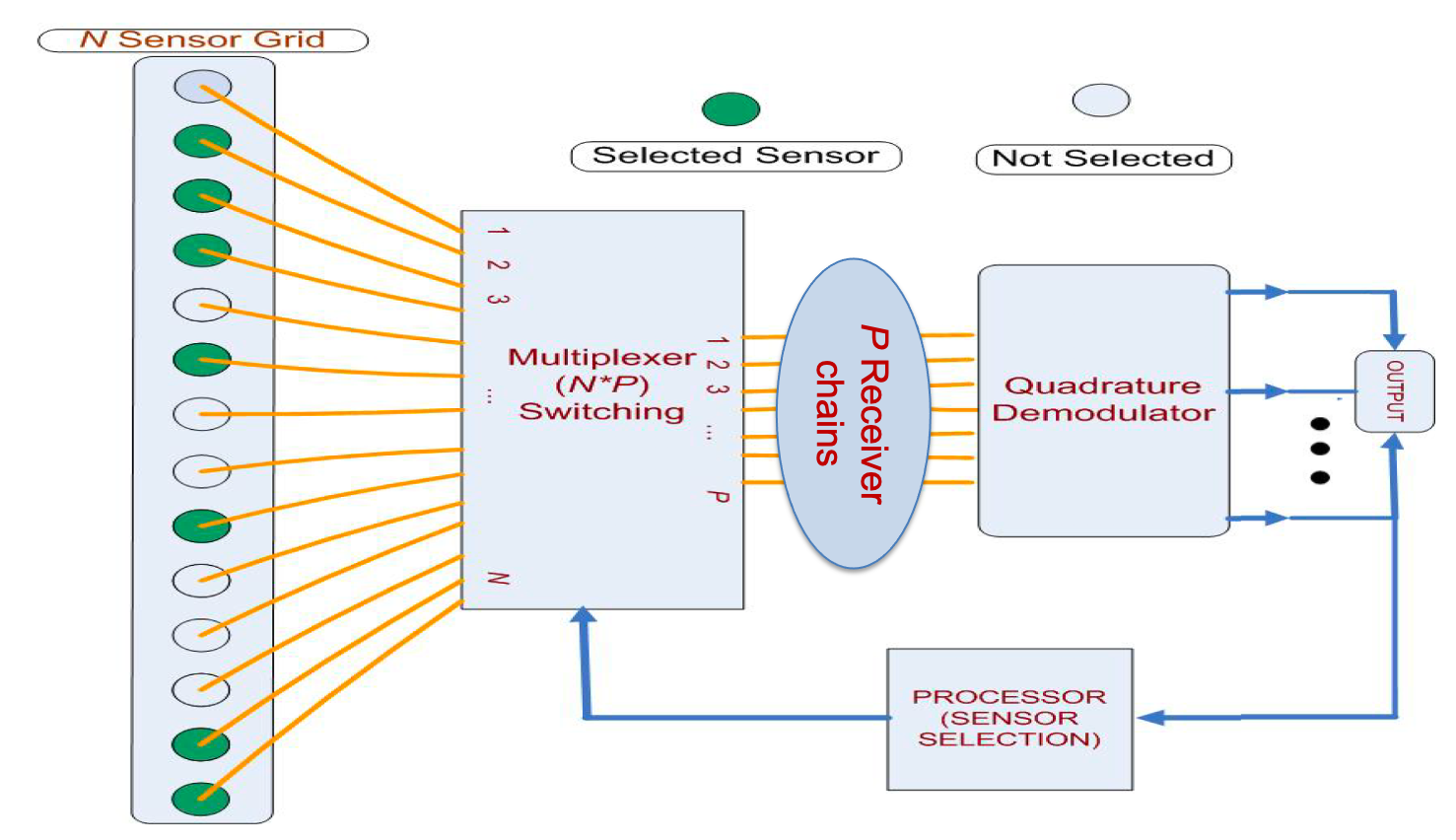
Figure 1: Block diagram of adaptive switched sensor beamformer

Main Contributions: The main contributions of this paper are,

1) Sparse beamformer spectral analysis (SBSA) algorithm is proposed which is computationally efficient and provides insights into MaxSINR beamformer design.

2) The DNN based approach is developed, for the first time, to configure a Capon based data driven sparse beamformer by learning the enumerated algorithm as well as SBSA design. The design is achieved through a direct mapping of the sensor data correlations to the optimum sparse array configuration for a given ‘look direction’. The proposed methodology utilizes the merits of the data dependent designs, through online implementation, and exploits the benefits of assuming prior information of the interfering environment by efficient training with low computational complexity.

The proposed design is shown to be robust to limited data snapshots and can be easily extended to robust adaptive beamforming to cater the uncertainty regarding the look direction DOA as well as array calibration errors.

The rest of the paper is organized as follows: In the next section, we state the problem formulation for maximizing the output SINR. Section III deals with the sparse array design by SBSA algorithm and section IV describes DNN based Capon implementation. In section V, with the aid of a number of design examples, we demonstrate the usefulness of proposed algorithms in achieving MaxSINR sparse array design. Concluding remarks follow at the end.

II Problem Formulation

The block digram of Fig. 1 depicts the essence of spare array beamforming. Dark circles indicated selected antennas that are connected to the front-end receivers through a multiplexing process. Consider a desired source and $L$ independent interfering sources whose signals impinge on a linear array with $N$ uniformly placed sensors. The baseband data received at the array at time instant $t$ is then given by,

$$\mathbf{x}(t)=(\alpha(t))\mathbf{s}(\theta)+\sum_{l=1}^{L}(\beta_{l}(t))\mathbf{v}(\theta_{l})+\mathbf{n}(t),$$ (1)

where, $\mathbf{s}({\theta_{k}})$ and $\mathbf{v}({\theta_{l}})$ $\in\mathbb{C}^{N}$ are the steering vectors corresponding to the direction of arrival, $\theta$ or $\theta_{l}$ of the desired source and $l$th interference, respectively, and are defined as follows,

$$\mathbf{s}({\theta})=[1\,\,\,e^{j(2\pi/\lambda)dcos(\theta)}\,.\,.\,.\,e^{j(2\pi/\lambda)d(N-1)cos(\theta)}]^{T}.$$ (2)

where $d$ is the inter-element spacing and ($\alpha(t)$, $\beta_{l}(t))$ $\in\mathbb{C}$ are the complex amplitudes of the incoming baseband signals [42]. The additive Gaussian noise $\mathbf{n}(t)$ $\in\mathbb{C}^{N}$ has variance $\sigma_{t}^{2}$. The elements of the received data vector $\mathbf{x}(t)$ are combined linearly by the $N$-sensor beamformer that strives to maximize the output SINR. The output signal $y(t)$ of the optimum beamformer for maximum SINR is given by [43],

$$y(t)=\mathbf{w}_{o}^{H}\mathbf{x}(t),$$ (3)

where $\mathbf{w}_{o}$ is the optimum weight vector resulting in the optimum output SINR_o,

$$\text{SINR}_{o}=\frac{\mathbf{w}_{o}^{H}\mathbf{R}_{s}\mathbf{w}_{o}}{\mathbf{w}_{o}^{H}\mathbf{R}_{s^{{}^{\prime}}}\mathbf{w}_{o}}.$$ (4)

For statistically independent signals, the desired source correlation matrix is $\mathbf{R}_{s}=\sigma^{2}\mathbf{s}(\theta)\mathbf{s}^{H}(\theta)$, where $\sigma^{2}=E\{\alpha(t)\alpha^{H}(t)\}$. Likewise, the interference and noise correlation matrix, $\mathbf{R}_{s^{{}^{\prime}}}=\sum_{l=1}^{L}(\sigma^{2}_{l}\mathbf{v}(\theta_{l})\mathbf{v}^{H}(\theta_{l})$) + $\sigma_{t}^{2}\mathbf{I}_{N\times N}$, with $\sigma^{2}_{l}=E\{\beta_{l}(t)\beta_{l}^{H}(t)\}$ being the power of the $l$th interfering source.

There exists a closed form solution to maximize the SINR expression in (4) and is given by $\mathbf{w}_{o}=\mathscr{P}\{\mathbf{R}_{s^{{}^{\prime}}}^{-1}\mathbf{R}_{s}\}=\mathscr{P}\{\mathbf{R_{xx}}^{-1}\mathbf{R}_{s}\}$ [43]. The operator $\mathscr{P}\{.\}$ computes the principal eigenvector of the input matrix. Substituting $\mathbf{w}_{o}$ into (4) yields the corresponding optimum output SINR_o,

$$\text{SINR}_{o}=\Lambda_{max}\{\mathbf{R}^{-1}_{s^{{}^{\prime}}}\mathbf{R}_{s}\}.$$ (5)

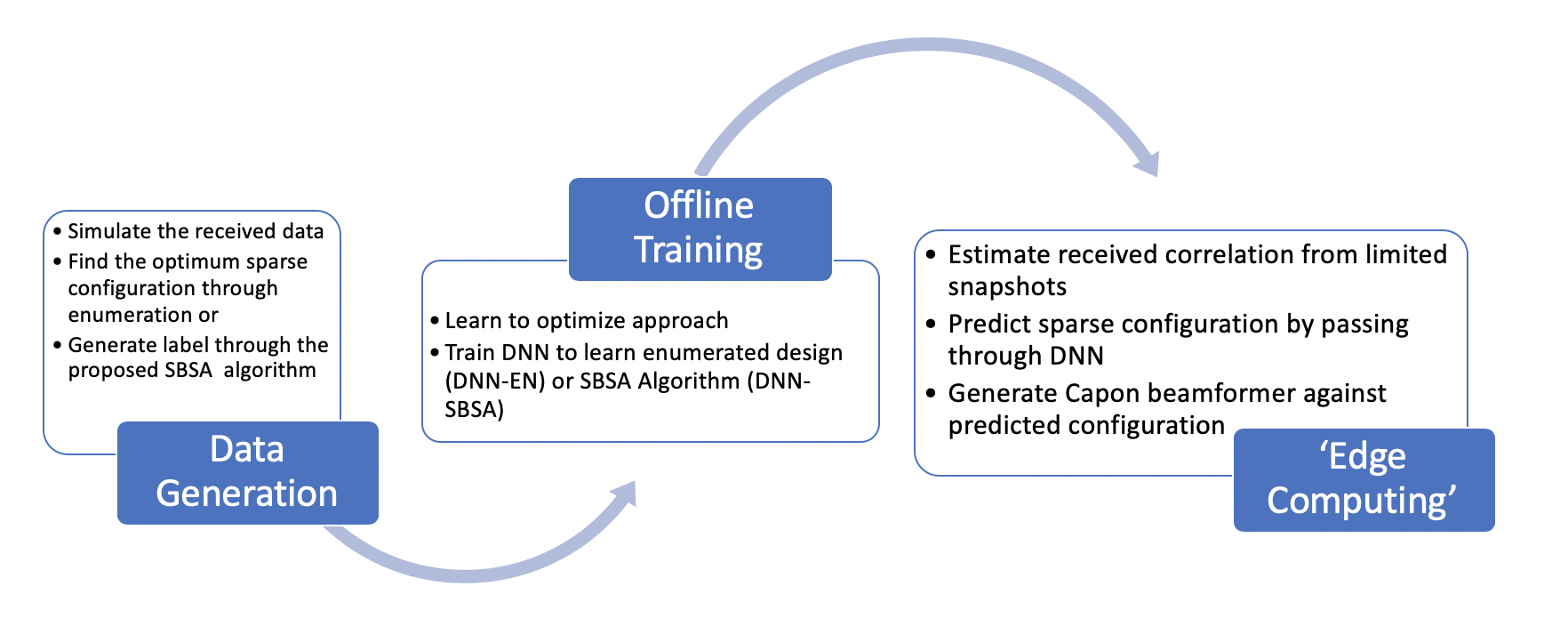
Figure 2: Overview of the proposed approach using Deep Neural Network (DNN)

Accordingly, the optimum output SINR_o is given by the maximum eigenvalue ($\Lambda_{max}$) associated with the product of the inverse of interference plus noise correlation matrix and the desired source correlation matrix. This is the general expression for point and distributed sources and give the similar expression in the point source case. Therefore, the performance of the optimum beamformer for maximizing the output SINR is directly related to the correlation matrix of the desired source and that of interference-plus-noise.

III Sparse array design

In order to maximize the SINR expression in (4), we constraint the numerator and minimize the denominator term as follows,

$$\underset{\mathbf{w}\in\mathbb{C}^{N}}{\text{minimize}} \quad\mathbf{w}^{H}\mathbf{R}_{s^{{}^{\prime}}}\mathbf{w},$$ (6)

s.t. $$\quad\mathbf{w}^{H}\mathbf{R}_{s}\mathbf{w}=1.$$

The problem in (6) can be written equivalently by replacing $\mathbf{R}_{s^{{}^{\prime}}}$ with the received data covariance matrix, $\mathbf{R_{xx}}=\mathbf{R}_{s}+\mathbf{R}_{s^{{}^{\prime}}}$ as follows [43],

$$\underset{\mathbf{w}\in\mathbb{C}^{N}}{\text{minimize}} \quad\mathbf{w}^{H}\mathbf{R_{xx}}\mathbf{w},$$ (7)

s.t. $$\quad\mathbf{w}^{H}\mathbf{R}_{s}\mathbf{w}\geq 1.$$

It is noted that the equality constraint in (6) is relaxed in (7) due to the inclusion of the constraint as part of the objective function, and as such, (7) converges to the equality constraint. Additionally, the optimal solution in (7) is invariant up to uncertainty in the absolute power of the desired source. In practice, the actual source parameters can deviate from the perceived ones. This discrepancy is typically mitigated, to an extent, by pre-processing the received data correlation matrix through diagonal loading or tapering the correlation matrix [14]. In order to bring aperture sparsity into optimum beamformer design, the constraint optimization (7) can be re-formulated by incorporating an additional constraint on the cardinality of the weight vector;

$$\underset{\mathbf{w\in\mathbb{C}}^{N}}{\text{minimize}} \quad\mathbf{w}^{H}\mathbf{R_{xx}}\mathbf{w},$$ (8)

s.t. $$\quad\mathbf{w}^{H}\mathbf{R}_{s}\mathbf{w}\geq 1,$$

$$\quad||\mathbf{w}||_{0}=P.$$

Here, $||.||_{0}$ determines the cardinality of the weight vector $\mathbf{w}$. This is a combinatorial optimization problem and can be solved by enumerating over all possible sensor locations. Several different approaches have been developed to mitigate the computational expense of the combinatorial search by either exploiting prior given information on the interference parameters, such as respective DOAs, or employing data-dependent algorithms realized through the SDR and SCA algorithms [15, 20]. These algorithms, however, have high computational costs, impeding real time implementations, especially in applications involving rapidly changing environments. In the context of designing sparse arrays using machine learning, the optimum sparse arrays for different operating environments constitute labels for the network training data. These labels can be generated off-line through enumerations, accounting for all possible source and interference scenarios. For large array, however, this approach becomes computationally challenging. In order to mitigate this problem, we propose an efficient technique to generate DNN training samples, using sparse beamformer spectral analysis (SBSA) design. This technique, detailed below, employs what is referred to as sparse beamformer spectral analysis (SBSA) design. It has desired performance and low computational complexity. The block diagram of Fig. 2 describes the three main steps in DNN-based sparse array design using training data generated by the SBSA and enumeration.

The Role of Spare Configuration in MaxSINR

As implied by (5), the optimum sparse array for MaxSINR design depends on both the beamforming weights and the sparse array configuration. Therefore, the problem of interference mitigation is not a cascade design of the optimum configuration followed by the optimum weights, or vice versa. Rather, it is an entwined task, in essence, calling for joint optimization of the beamforming weights and sparse array configuration. Albeit not optimum, the cascade design approach is not entirely without merits. It can offer a unique insight into the problem and address the suitability of a given sparse array configuration in canceling the interfering signals.

In order to shed more light on the role of array configuration in optimum sparse beamforming, we recognize that the problem formulation developed in the previous section is valid irrespective of the array configuration and holds true for the compact ULA or any generic sparse configuration. The beamformer output signal, $y(t)={\mathbf{w}}^{H}\mathbf{x}$, for a sparse beamformer can also be written as $\overset{\circ}{y}(t)=\overset{\circ}{\mathbf{w}}^{H}\mathbf{x}$, where the typeset ‘${{\circ}}$’ indicates that the corresponding vector is sparse with few zero entries. The sparse beamformer $\overset{\circ}{y}(t)$ can be rewritten, equivalently, as $\overset{\circ}{y}(t)=\overset{\circ}{\mathbf{w}}^{H}\{\overset{\circ}{\mathbf{z}}\odot\mathbf{x}\}$. The entries of $\overset{\circ}{\mathbf{z}}\in\mathbb{R}^{N}$ are either 1’s or 0’s depending on whether the corresponding sensor location is active or inactive respectively. The point-wise multiplication ($\odot$) of the received vector $\mathbf{x}$ with a sparse selection vector $\overset{\circ}{\mathbf{z}}$ sets the corresponding entries of the received signal to zero which amounts to the zero beamforming weights of $\overset{\circ}{\mathbf{w}}$.

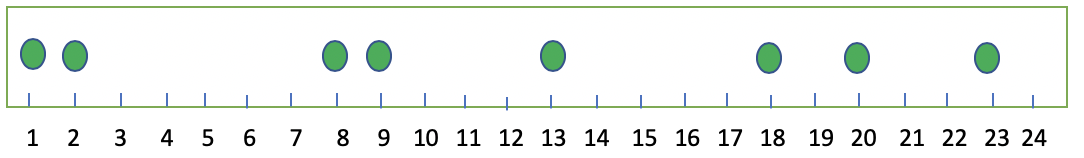
Figure 3: Eight element sparse array configuration

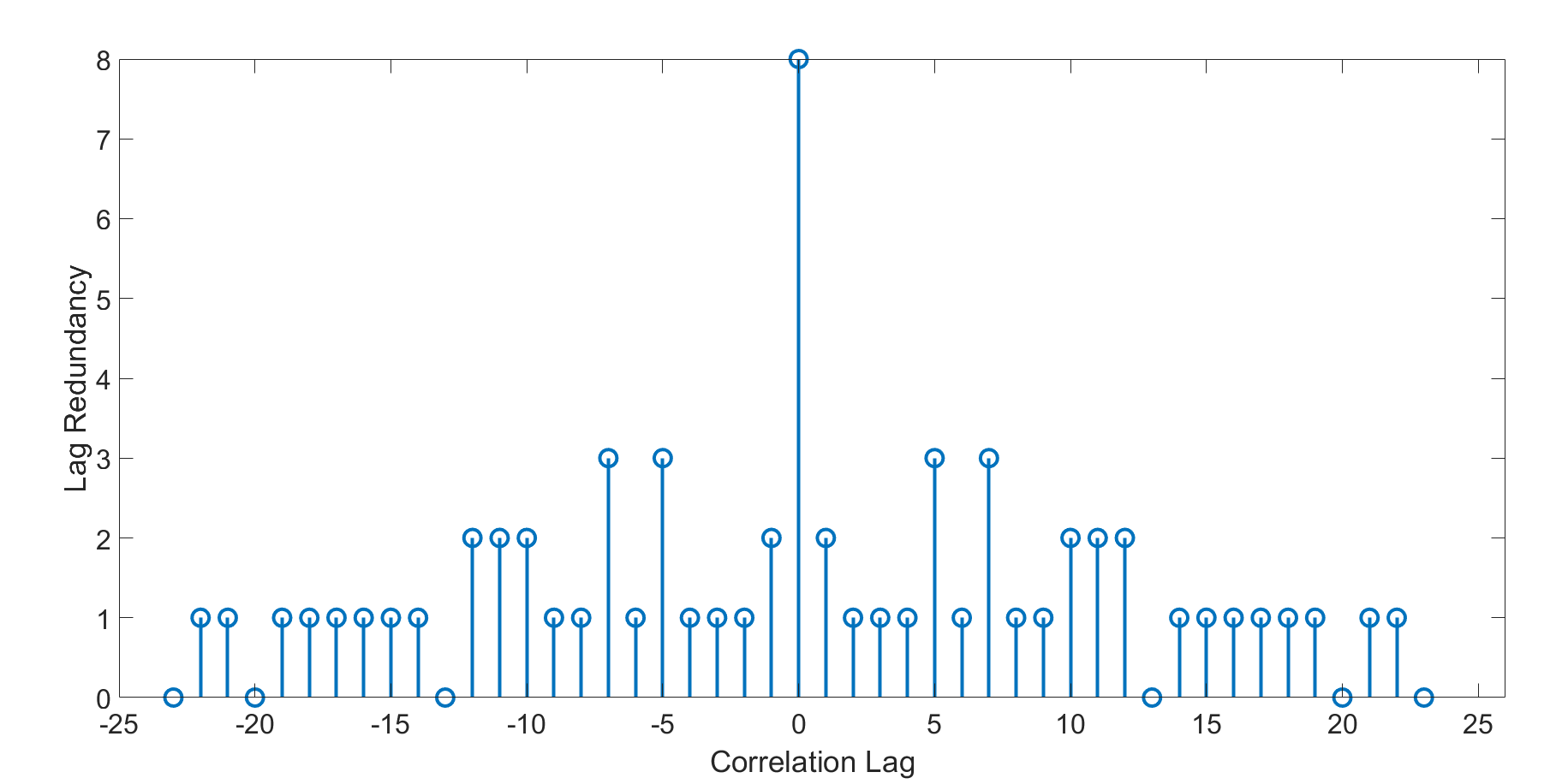
Figure 4: Lag Redundancy of the sparse array shown in Fig. 3

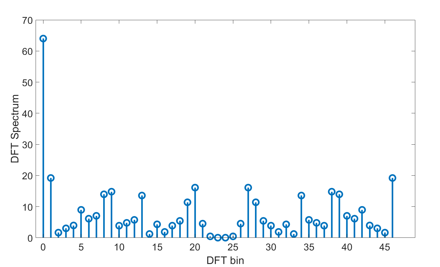
Figure 5: DFT of the lag redundancy

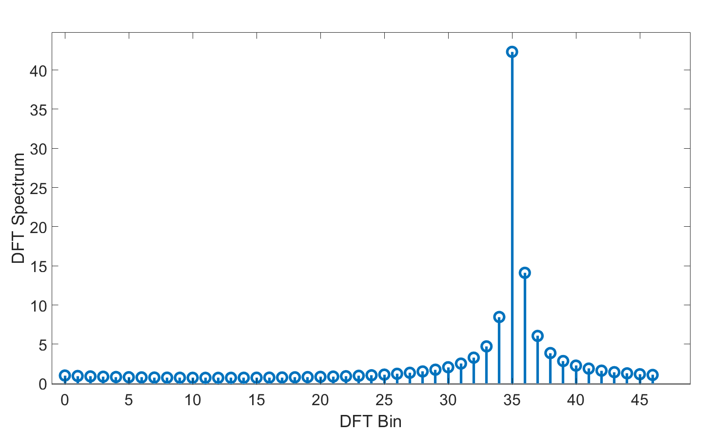
Figure 6: Power spectrum of the desired signal

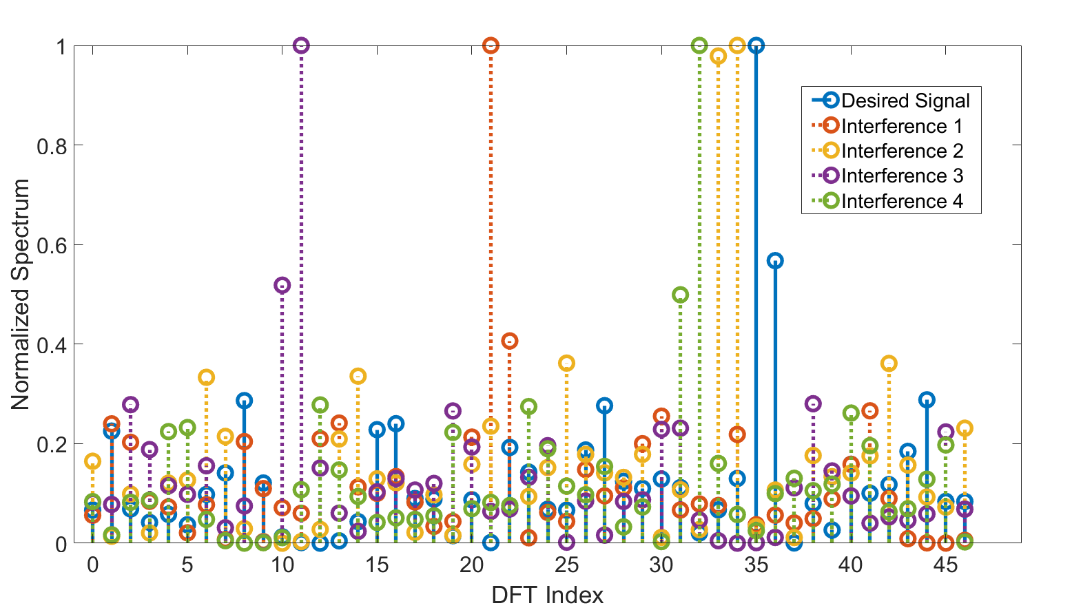
Figure 7: Explanation of the proposed objective criterion for the optimum array configuration shown in Fig. 3

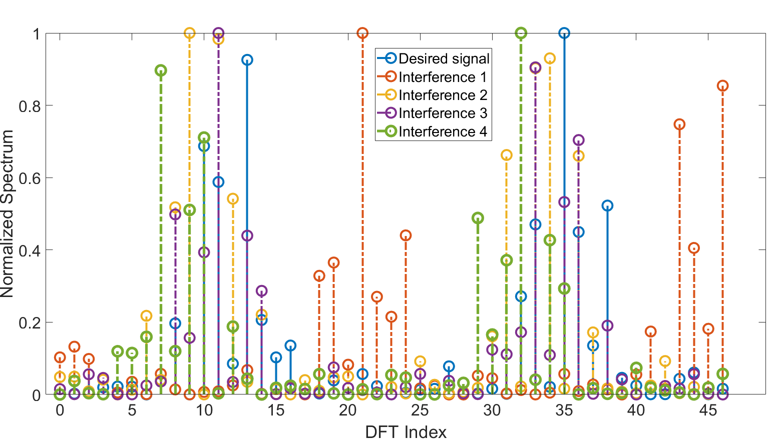
Figure 8: Explanation of the proposed objective criterion for the worst possible array configuration

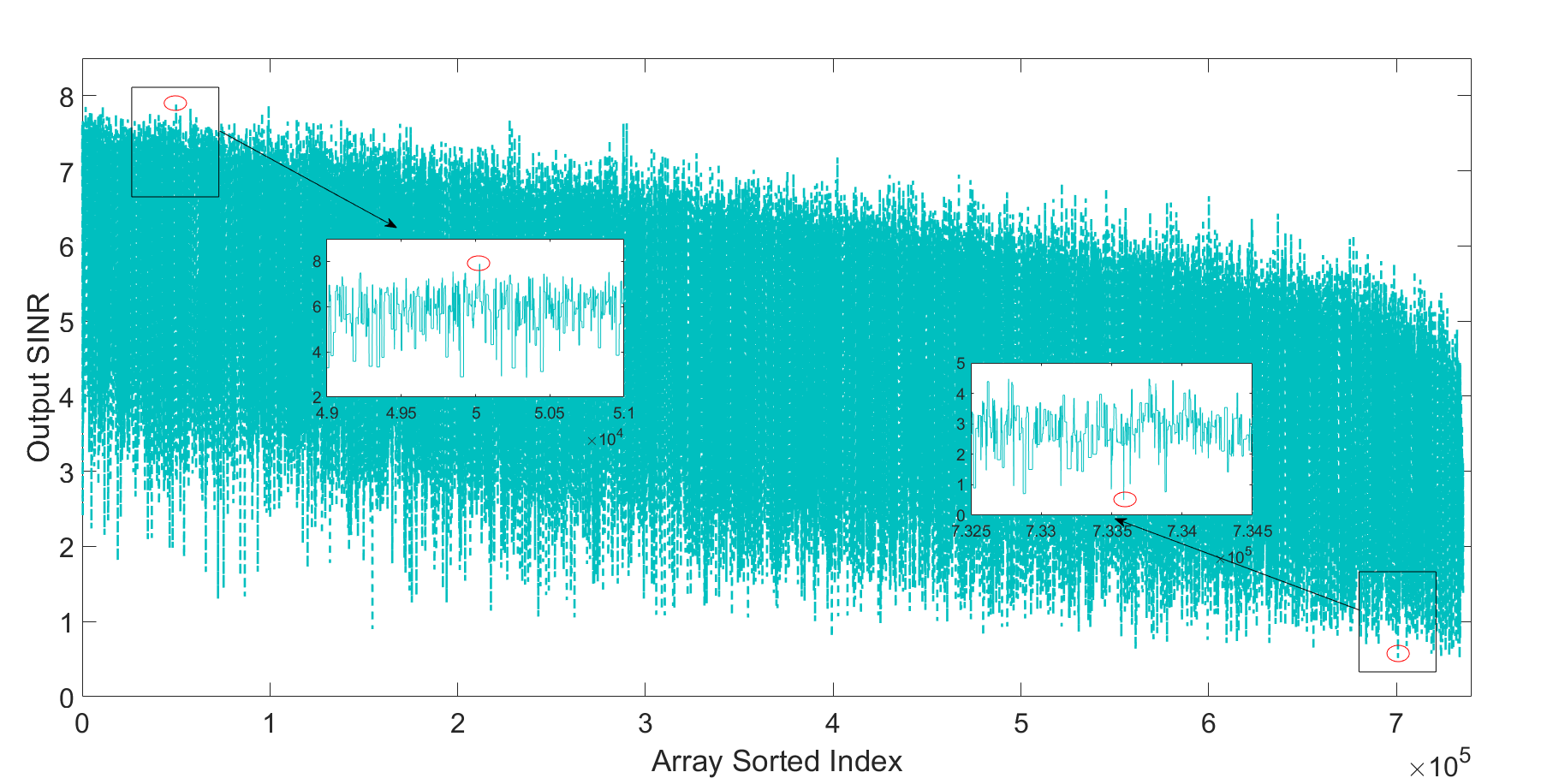
Figure 9: Plot of the proposed objective criterion in ascending order

Therefore, sparse beamforming can be viewed as pre-processing the received signal by point-wise multiplication, prior to applying the optimum weights. We analyze the impact of such multiplication on the performance of the subsequent, or cascade, design of the beamformer weights, $\overset{\circ}{\mathbf{w}}$.

Let $\mathbf{X}=\mathscr{F}(\mathbf{x})$ and $\mathbf{Z}=\mathscr{F}(\overset{\circ}{\mathbf{z}})$ denote the DFT of the input data and the selection vector, respectively. The DFT of the point-wise multiplication of these two vectors is given by the circular convolution of the corresponding DFTs, i.e., $\mathscr{F}(\overset{\circ}{\mathbf{z}}\odot\mathbf{x})=\mathbf{X}\circledast\mathbf{Z}$, where $\circledast$ denotes circular convolution. From (1) and the linearity property of DFT, we obtain $\mathscr{F}(\overset{\circ}{\mathbf{z}}\odot\mathbf{x})=\alpha\mathbf{S}\circledast\mathbf{Z}+\sum_{l=1}^{L}\beta_{l}\mathbf{V}_{l}\circledast\mathbf{Z}+\mathbf{N}\circledast\mathbf{Z}$, where $\mathbf{V}_{l}$ is the DFT of the $l$th interference vector. The $N$ components of $\mathbf{X}$ represent orthogonal beamformers, each pointing towards a certain spatial direction. The convolution with $\mathbf{Z}$ alters these components as well as changes the contribution of the $l$th interference to the signal received from the desired source location. The proposed scheme gauges the overlap between the spatial spectra of the desired signal and the interfering signals as a function of the underlying sparse configuration. A desirable array configuration would minimize such overlapping, enabling the beamformer weights to effectively remove the interference, while maintaining the desired signal. Towards this end, we propose a design metric $\Omega(\mathbf{Z})$ based on weighted sum of the spatial spectrum (denoted by $|.|^{2}$) of the individual interfering sources scaled by the desired signal spatial spectrum as follows,

$$\Omega(\mathbf{Z})=\sum_{l=1}^{L}\{\alpha^{2}|\mathbf{S}\circledast\mathbf{Z}|^{2}\}\odot\{\beta_{l}^{2}|\mathbf{V}_{l}\circledast\mathbf{Z}|^{2}\}$$ (9)

Eq. (9) performs element-wise scaling of the interfering powers in the DFT domain. Therefore, if the interfering signal power, after convolution is concentrated in the DFT bins different from those occupied primarily by the desired signal, then the point-wise product would assume low values. Conversely, if there is a significant overlap between the results of the two convolutions, then the objective function $\Omega(\mathbf{Z})$ is significantly higher.

The spatial spectrum can be estimated by computing the DFT of the autocorrelation function of the corresponding signal. It is worth noting that, for a given sparse configuration, the autocorrelation function of the selection vector assumes a specific redundancy of the autocorrelation lags. Therefore, unlike the structured sparse array design that seeks to maximize the contiguous correlation lags, MaxSINR sparse design is guided by the DFT of the autocorrelation sequence of the lag redundancy.

We illustrate the proposed approach with the help of the following example. Consider an 8-element sparse array on the 24 point equally spaced grid locations that are potentially available for sensor selections. The minimum spacing among the sensors is $d=\lambda/2$. Consider a source signal located at $60^{0}$ and four unwanted interferences located at $154^{0}$, $55^{0}$, $117^{0}$ and $50^{0}$ with the INRs ranging from $10-20$ dB. The sparse array configuration achieving the best SINR performance is found through enumeration and shown in Fig. 3. The associated correlation lag redundancy of this configuration and the corresponding spatial spectrum are depicted in Figs. 4 and 5, respectively. The spatial spectrum of the desired source at $60^{0}$ prior to convolution is depicted in the Fig. 6. The normalized result of the two convolved spectra in Figs. 5, 6 is shown as solid lines (blue) in the Fig. 7. The normalized spectrum for each interfering signal is also shown as dotted lines in the same figure. Fig. 8 plots the normalized spectrum for the sparse array worst case scenario for comparison purposes. Note that the maximum of the convolved desired signal spectrum occurs at 35th DFT bin. For the best case scenario, all convolved interfering signals assume minimum power at the aforementioned DFT position. This is in contrast to the worst case scenario where there is considerable interference power at the peak of the desired source. Apart form the maximum location, it is noted that for the best case design, there is minimum overlapping between the desired signal and interfering signals at the DFT bin locations which is clearly in contrast to the worst case design.

In order to further understand the offerings of the proposed approach, Fig. (9) plots the SINR performance of all possible sparse configurations after sorting the array configurations in ascending order of the output of the proposed objective function of (9). It is clear that the average SINR in the plot is higher and more desirable towards the left side where the objective function is minimum. It is important to note that the best enumerated result of MaxSINR performance does not correspond to the array configuration with the smallest objective function. This is because, the optimum sparse configuration also depends on the beamformer weights to minimize the interfering signals. This is also clear from the high variance of the curve. Similarly, the worst performing array is very close to the right side of the curve where the proposed objective function is high due to the strong overlap of the desired and undesired signal spectra.

For efficient generations of DNN training data and in lieu of enumerations, the objective function (9) can be minimized through an iterative algorithm that implements successive sensor selections, hence deciding on one sensor location at a time. For the initial iteration, a sensor location is chosen randomly on an $N$ grid points. For the $i$th subsequent iteration, the proposed objective is evaluated at the remaining $N-i$ locations and then selecting the sensor location that yields the minimum objective function. The procedure is iterated $P$ times for selecting the $P$ locations from $N$ possible locations. Due to high variance of the curve in Fig. 10, it is best to initialize the algorithm with different sensor location and find the corresponding configurations for each initialization, and eventually consider the one with the best SINR performance. The steps of the above algorithm are detailed in Algorithm 1. It is noted that aside from the efficient generations of DNN training data in the underlying problem, this approach can itself be used in general as a stand alone method to determine appropriate array configurations if prior information of the interference parameters is provided.

Algorithm 1 SBSA Algorithm

Input: $N$, $P$, Look direction DOA $\theta$, Interference DOAs, SNR and INRs
Output: Sparse beamformer $\mathbf{w}_{o}$
Initialize $\mathbf{z}$=$[0\,\,1\,\,0\,...\,0]$ where all entries of $\mathbf{z}$ are zero except an arbitrarily selected entry.
Compute the spatial spectrum of desired source and interfering signals.
for    j=1 to $P$-1
for    i=1 to $P$-1-j
Select the ith sensor from $P$-1-j remaining locations.
Compute the lag redundancy of this sparse array consisting of j+1 sensor.
Compute the spatial spectrum of the j+1 sensor sparse array.
Convolve the spatial spectrum of the j+1 sensor sparse array with the spectrum of the desired source and the interfering sources.
Compute the overlapping power in the spatial spectra by computing the proposed metric in (9).
end for
Select the $i$th sensor from the inner for loop which results in the minimum overlapping power computed by (9).
Update $\mathbf{z}$ by setting the jth location in $\mathbf{z}$ to 1.
end for
After finding the sparse configuration find $\mathbf{w}_{o}$ by running (7) for reduced size correlation matrix while ignoring the sensor locations corresponding to $\mathbf{z}$.

IV DNN based learning of the SBSA and enumerated designs

Modeling the behaviour of optimization algorithms by training a DNN is justifiable, as DNNs are universal approximators for arbitrary continuous functions and have the required capacity to accurately map almost any input/output formula. For effective learning, it is important that the DNN can generalize to a broader class than that represented by the finite number of drawn training examples. From the Capon beamforming perspective, a given arrangement of a desired source direction, interference DOAs and respective SNR/INRs constitute just one particular example. A class, in this case, is defined by any arbitrary permutation of the interference DOAs and respective powers while keeping the desired source DOA fixed. The DNN task is, therefore, to learn from a data-set, characterized by a set of different training examples and corresponding optimum sparse array predictions.

Here, an important question arises as whether we could aim for a stronger notion of generalization, i.e., instead of training for a fixed desired source, is it possible to generalize over all possible desired source DOAs. To answer this query, we note that for a given desired source and interference setting, the received array data, and thereby the data correlation, remains the same even if we switch the desired signal and one of the interferers. However, Capon beamformer should yield a different configuration due to changing its directional constraint. Therefore, instead of relying entirely on the information of the received data correlation, it is imperative to incorporate the knowledge of the desired source or look direction, which is always assumed in Capon beamforming formulation. For DNN learning, this information can either be incorporated by exclusively training the DNN for each desired source DOA or the desired source DOA can be incorporated as an additional input feature to DNN. In this paper, we adopt the former approach.

For DNN, we use multilayer perceptron (MLP) network, as shown in Fig. 10. The input layer is of size $2N-1$ and the output layer is of size $N$. Although there are $N$ unique correlation lags ($\mathbf{r_{x}}(n-1)=\mathbf{R_{xx}}(1,n)$) corresponding to the $N$ sensor locations on the grid, the dimensionality of the input layer is $2N-1$ owing to concatenating the real and imaginary entries of the generally complex valued correlation lags, except the zeroth lag. We use 3 hidden layers with 450, 250 and 80 nodes, respectively. The ReLU activation function is used for all hidden layers activation. The correlation values of the received data assuming a stationary environment are input to the network. The network output $\mathbf{z}$ is a binary vector such that 1 indicate sensor selection and 0 indicates the absence of the corresponding sensor location.

The received data is generated in the following manner. For a given desired source location, the $i$th training realization is simulated by randomly selecting $L$ interfering signals from a DOA grid spanning the range of $10^{0}$ to $170^{0}$, with a grid spacing of $1^{0}$. The interferers are allocated random powers uniformly distributed with INR from 10 dB to 20 dB. For this given scenario, the received correlation function, which includes the desired source signal, is calculated corresponding to the full sensor configuration. The corresponding optimum configuration is found through enumeration and also through the proposed SBSA algorithm. The process is repeated 30000 times against a given desired source DOA to generate the training data set. Similarly, a small sized validation data set is generated for hyperparamter tuning for model selection, minibatch size and learning rate.

For the training stage, the weights of the neural network are optimized to minimize the mean squared error between the label and the output of the network. The ADAM algorithm is used to carry out parameter optimization, employing efficient implementation of mini-batch stochastic gradient descent algorithm [44]. The learning rate is set to 0.001 and dropout regularization with the keep probability of 0.9 is used. The weights are initialized using the Xavier initialization. We chose MLP as DNN for its simplicity. In essence, MLP presents the baseline with other networks, such as Convolutional Neural Networks, are slated to give better performance with sufficiently large training data [45, 46].

The robustness of the learned models is demonstrated by generating the test data that is different from the training stage, by assuming the DOA of the interfering signals off grid. This is simulated by adding the Gaussian noise to the interference DOAs on the grid. We also present the results under limited and unlimited data snapshots. The sparse array design can only have few active sensors at a time, in essence, making it difficult to furnish the correlation values corresponding to the inactive sensor locations. However, for the scope of this paper, we assume that an estimate of all the correlation lags corresponding to the full aperture array are available to input for prediction. This can typically be achieved by employing a low rank matrix completion strategy that permits the interpolation of the missing correlation lags [8]. Additionally, to ensure the selection of $P$ antenna locations at the output of DNN, we declare the $P$ highest values in the output as the selected sensor locations. Therefore, generalization in this context means that the learned DNN works on different interference settings which can change according to changing environment conditions.

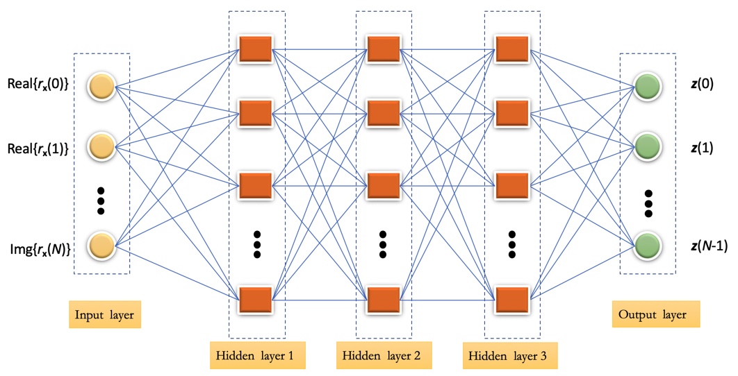
Figure 10: Architecture of Deep Neural Network (DNN)

V Simulations

In this section, we show the effectiveness of the proposed approach for sparse array design achieving MaxSINR. The results are examined first by training the DNN to learn the enumerated optimum array configurations. Then, we demonstrate in the follow-on examples the effectiveness of the DNN when trained by the labels drawn from SBSA algorithm.

V-A Enumerated design

In this example, we pose the problem as selecting $P=6$ antennas from $N=12$ possible equally spaced locations with inter-element spacing of $\lambda/2$. For all numerical results, we use a network with three hidden layers, one input layer, and one output layer. Accordingly, the input to the network is of size 23 and output is size 12.

Figure 11 shows the output SINR performance comparisons for different array configurations. The horizontal axis is the DOA of the desired point source, and the performance is computed at six different source DOAs varying from $15^{0}$ to $90^{0}$ in steps of $15^{0}$. The SNR of the desired signal is set to $0$ dB, whereas the interference-to-noise-ratio (INR) for each interference is chosen randomly between $10-20$ dB for a given realization. The results presented in Fig. 11 are obtained by using unlimited number of data snapshots (USS), i.e., exact spatial correlation values, and employing enumerated labels to train the DNN. This approach is referred to as DNN-EN. The network performance is reported by averaging over $900$ testing scenarios for each desired source DOA. It is evident that the DNN-EN approach performs close (0.45 dB trade off) to the performance of the optimum array found by enumeration. The latter amounts to trying all 980 configurations and choosing the one with the highest SINR. It involves expensive singular value decomposition (SVD) for each enumeration and is also not scale-able with the problem size, facing the curse of dimensionality.

The DNN-EN design performance is also compared with the simple NNC (nearest neighbour correlation) design which returns the label corresponding to the input nearest neighbour correlation function (in terms of mean square error). NNC design is essentially a lookup table, such that for a given test data, it returns the label of the closest training example by sifting through the entire training set. It is noted that the DNN-EN design outperforms the NNC design, which does not involve DNN processing, with an average performance gain of 0.5 dB. The former approach not only offers superior performance but also is more economically viable from ‘Edge computing’ perspective. It is noted that the nearest neighbour design requires maintaining a large dictionary and run exhaustive search over the entire training set for each prediction. Similar results are obtained for the NNC design where we minimize the mean absolute error in lieu of the mean square error. For the underlying case, the DNN-EN approach has around 88$\%$ accuracy for the training data, and has around 54$\%$ accuracy on the test data (meaning that 54$\%$ of the times all $P$ sensor locations are correctly predicted). This is significant since there are $980$ possible permutations for a given example. It is noted that the superior performance of the DNN (shown in Fig. 11) is not simply because it recovered the optimal solution for 54$\%$ of the cases, but also it yielded superior SINR performing configurations for the majority of the remaining 46$\%$ sub optimal solutions. This is due to the network ability to generalize the learning as applied to the test set not present in the training data. The superior performance of DNN over NNC design reveals that the DNN doesn’t memorize a lookup table implementation to locate the nearest training data point and output the corresponding memorized optimal sparse configuration. It is clear from Fig. 11 that the proposed design yields significant gains over a compact ULA, sparse ULA and randomly selected array topology. The utility of the effective sparse design is also evident from observing the worst case performance which exhibits significantly low output SINR of around -5 dB on average.

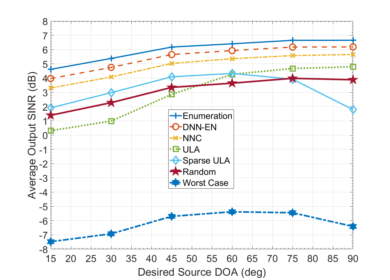
Figure 11: Performance comparison of enumerated design under unlimited snapshots

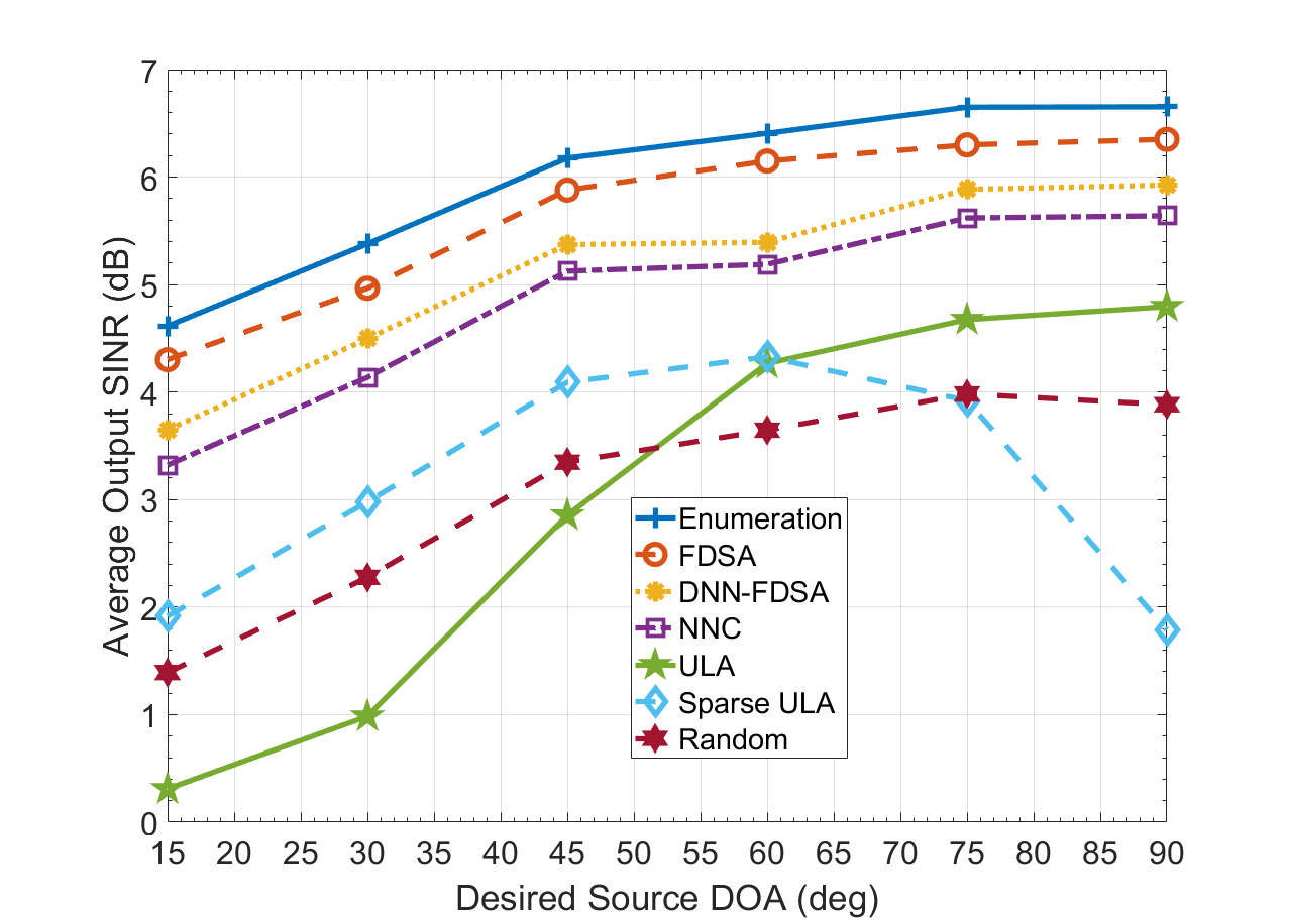
Figure 12: Performance comparison of SBSA design under unlimited snapshots

V-B DNN based SBSA design

Although the training phase is entirely offline, it is infeasible to train the DNN relying on the enumerated results. This is because the number of possible sparse solutions can be considerably large even for modest size arrays. For instance, choosing 14 elements out of 24 possible locations results in the order of $10^{6}$ candidate spare configurations for each training data, i.e., for each environment scenario. In order to avoid this problem and generate a large amount of training data labels, we resort to the proposed SBSA design. Fig. 12 shows the performance of SBSA design which is merely 0.3 dB down from that of the design obtained through enumeration. Quite similar to the DNN-EN design (0.4 dB down from enumerated design), the DNN-SBSA design is around 0.38 dB down from SBSA design. This places the DNN-SBSA design 0.68 dB suboptimal to the enumerated design in aggregate. However, it is still a reasonable performance yielding significant dividends over the commonly used compact ULA, sparse ULA and random sparse topology, as illustrated in the figure.

V-C Robust design

In order to gauge the robustness of the DNN based scheme, the performance is evaluated under a limited number of data snapshots. Also, the desired source DOA is perturbed with Gaussian noise of zero mean and 0.25⁰ variance to account for possible uncertainty around the desired source DOA. For simulating the limited snapshot scenario, 512 snapshots are generated assuming the incoming signals (source and interfering signals) are independent BPSK signals in the presence of Gaussian noise. The correlation matrix under limited snapshots doesn’t follow the Toeplitz structure. Therefore, we average the entries along the diagonal and sub-diagonals of the correlation matrix to calculate the average values. Figs. 13 and 14 show the performance of DNN-EN and DNN-SBSA designs under limited data snapshots. It is clear from the figures that the performance is largely preserved with an SINR discrepancy of less than 0.01 dB demonstrating the robustness of the proposed scheme. The NNC design, in this case, is suboptimal with more than 0.3 dB additional performance loss.

V-D Performance comparisions with state-of-the-art

The performance of the proposed SBSA, DNN-EN and DNN-SBSA are compared with existing work on sparse array design which is based on SDR and SCA approaches [19, 20]. It is clear from Fig. 15 that the SBSA algorithm outperforms the other designs and is also more than 100X computationally efficient as compared to the SDR and SCA (Wang etal. [19]) approaches. However, it is only fair to compare the SBSA design with the SCA (Wang etal.) approach because both incorporate the apriori knowledge of interference parameters. Therefore, in comparing the data dependent designs, it is found that SDR design (also the SDR-symmetric [20]) is comparable to the DNN-EN design, with the DNN-SBSA is marginally suboptimal with the average performance degradation of 0.37 dB. This slight performance trade off is readily leveraged by the real time realization of the DNN-SBSA algorithm implementing the Capon beamformer in time frames of the order of few milli-seconds.

VI Conclusion

This paper considered sparse array design for maximizing the beamformer output SINR for a desired source in an interference active scenario. A sparse beamformer spectral analysis (SBSA) algorithm was proposed which provided an insightful perspective of the role of array configuration in MaxSINR beamforming. A DNN based approach was developed to configure a data-driven sparse beamformer by learning the enumerated design as well as SBSA design. We employed MLP- DNN for its simplicity and limited training data requirements. Other networks with complex structures, like CNN, can yield better performance with larger training data set. The proposed methodology harvests the merits of both the data dependent array designs and designs assuming prior information of interference parameters. It was shown through design examples that the proposed schemes promise optimal solution for around 54$\%$ of the test scenarios and located superior sub-optimal sparse configurations, in terms of SINR performance, for the remaining 46$\%$. The proposed approach is robust against limited data snapshots and promise high performance with reduced computational complexity.

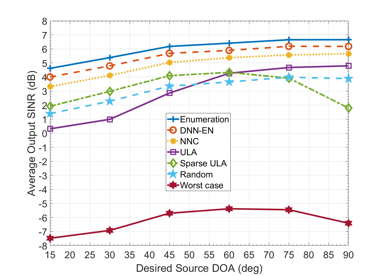
Figure 13: Performance comparison of enumerated design under 512 snapshots

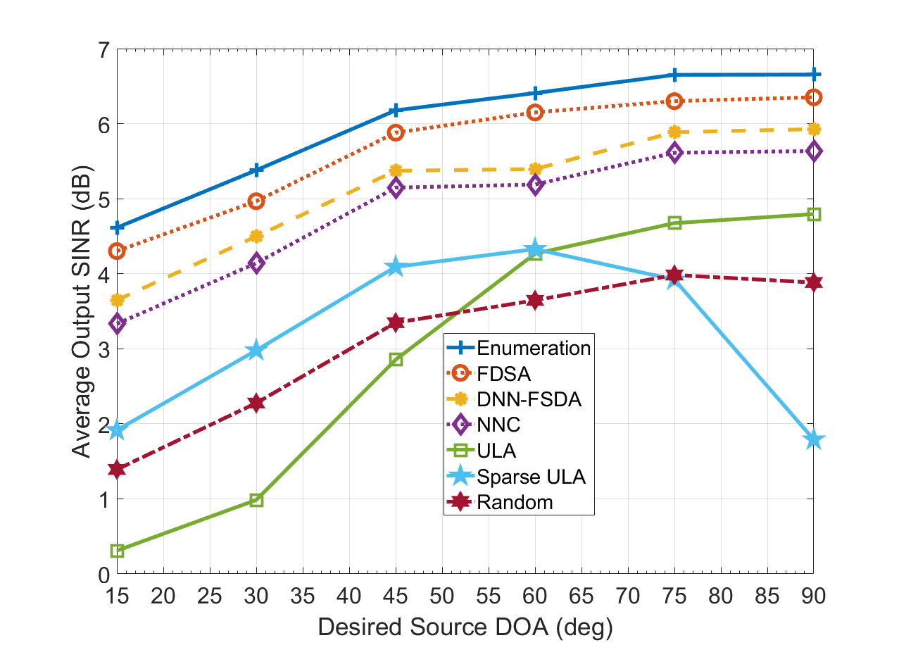
Figure 14: Performance comparison of SBSA design under 512 snapshots

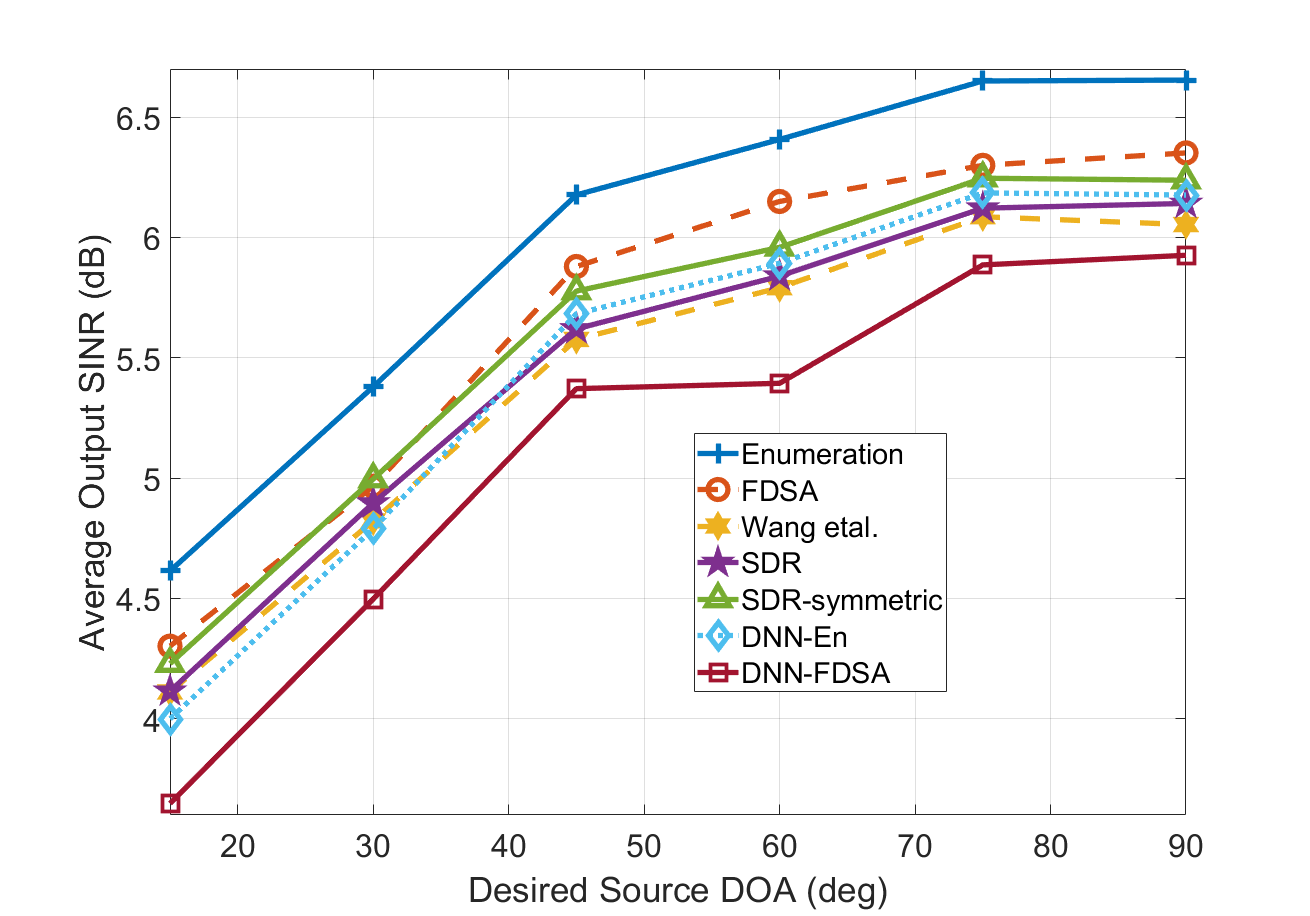
Figure 15: Performance comparisons with the state-of-the-art

References

- [1] G. R. Lockwood, J. R. Talman, and S. S. Brunke, “Real-time 3-D ultrasound imaging using sparse synthetic aperture beamforming,” IEEE Transactions on Ultrasonics, Ferroelectrics, and Frequency Control, vol. 45, no. 4, pp. 980–988, July 1998.
- [2] O. Mehanna, N. D. Sidiropoulos, and G. B. Giannakis, “Joint multicast beamforming and antenna selection,” IEEE Transactions on Signal Processing, vol. 61, no. 10, pp. 2660–2674, May 2013.
- [3] Y. He and K. P. Chong, “Sensor scheduling for target tracking in sensor networks,” in 2004 43rd IEEE Conference on Decision and Control (CDC) (IEEE Cat. No.04CH37601), vol. 1, Dec 2004, pp. 743–748 Vol.1.
- [4] W. V. Cappellen, S. J. Wijnholds, and J. D. Bregman, “Sparse antenna array configurations in large aperture synthesis radio telescopes,” in 2006 European Radar Conference, Sept 2006, pp. 76–79.
- [5] S. Joshi and S. Boyd, “Sensor selection via convex optimization,” IEEE Transactions on Signal Processing, vol. 57, no. 2, pp. 451–462, Feb 2009.
- [6] H. Godrich, A. P. Petropulu, and H. V. Poor, “Sensor selection in distributed multiple-radar architectures for localization: A knapsack problem formulation,” IEEE Transactions on Signal Processing, vol. 60, no. 1, pp. 247–260, Jan 2012.
- [7] M. G. Amin, P. P. Vaidyanathan, Y. D. Zhang, and P. Pal, “Editorial for coprime special issue,” Digital Signal Processing, vol. 61, no. Supplement C, pp. 1 – 2, 2017, special Issue on Coprime Sampling and Arrays.
- [8] S. A. Hamza and M. G. Amin, “Sparse array design for maximizing the signal-to-interference-plus-noise-ratio by matrix completion,” Digital Signal Processing, p. 102678, 2020. [Online]. Available: http://www.sciencedirect.com/science/article/pii/S1051200420300233
- [9] A. Moffet, “Minimum-redundancy linear arrays,” IEEE Transactions on Antennas and Propagation, vol. 16, no. 2, pp. 172–175, March 1968.
- [10] P. Pal and P. P. Vaidyanathan, “Nested arrays: A novel approach to array processing with enhanced degrees of freedom,” IEEE Transactions on Signal Processing, vol. 58, no. 8, pp. 4167–4181, Aug. 2010.
- [11] S. Qin, Y. D. Zhang, and M. G. Amin, “Generalized coprime array configurations for direction-of-arrival estimation,” IEEE Transactions on Signal Processing, vol. 63, no. 6, pp. 1377–1390, March 2015.
- [12] A. Goldsmith, Wireless Communications. New York, NY, USA: Cambridge University Press, 2005.
- [13] H. L. V. Trees, Detection, Estimation, and Modulation Theory: Radar-Sonar Signal Processing and Gaussian Signals in Noise. Melbourne, FL, USA: Krieger Publishing Co., Inc., 1992.
- [14] J. Li, P. Stoica, and Z. Wang, “On robust Capon beamforming and diagonal loading,” IEEE Transactions on Signal Processing, vol. 51, no. 7, pp. 1702–1715, July 2003.
- [15] X. Wang, E. Aboutanios, M. Trinkle, and M. G. Amin, “Reconfigurable adaptive array beamforming by antenna selection,” IEEE Transactions on Signal Processing, vol. 62, no. 9, pp. 2385–2396, May 2014.
- [16] N. D. Sidiropoulos, T. N. Davidson, and Z.-Q. Luo, “Transmit beamforming for physical-layer multicasting,” IEEE Transactions on Signal Processing, vol. 54, no. 6, pp. 2239–2251, June 2006.
- [17] V. Roy, S. P. Chepuri, and G. Leus, “Sparsity-enforcing sensor selection for DOA estimation,” in 2013 5th IEEE International Workshop on Computational Advances in Multi-Sensor Adaptive Processing (CAMSAP), Dec. 2013, pp. 340–343.
- [18] X. Wang, M. G. Amin, X. Wang, and X. Cao, “Sparse array quiescent beamformer design combining adaptive and deterministic constraints,” IEEE Transactions on Antennas and Propagation, vol. PP, no. 99, pp. 1–1, 2017.
- [19] X. Wang, M. Amin, and X. Cao, “Analysis and design of optimum sparse array configurations for adaptive beamforming,” IEEE Transactions on Signal Processing, vol. PP, no. 99, pp. 1–1, 2017.
- [20] S. A. Hamza and M. G. Amin, “Hybrid sparse array beamforming design for general rank signal models,” IEEE Transactions on Signal Processing, vol. 67, no. 24, pp. 6215–6226, Dec 2019.
- [21] J. Sheinvald and M. Wax, “Direction finding with fewer receivers via time-varying preprocessing,” IEEE Transactions on Signal Processing, vol. 47, no. 1, pp. 2–9, Jan 1999.
- [22] Y. Asano, S. Ohshima, T. Harada, M. Ogawa, and K. Nishikawa, “Proposal of millimeter-wave holographic radar with antenna switching,” in 2001 IEEE MTT-S International Microwave Sympsoium Digest (Cat. No.01CH37157), vol. 2, May 2001, pp. 1111–1114 vol.2.
- [23] Li Yang, Liang Liwan, Pan Weifeng, Chen Yaqin, and Feng Zhenghe, “Signal processing method for switch antenna array of the FMCW radar,” in Proceedings of the 2001 IEEE Radar Conference (Cat. No.01CH37200), May 2001, pp. 289–293.
- [24] Moon-Sik Lee, V. Katkovnik, and Yong-Hoon Kim, “System modeling and signal processing for a switch antenna array radar,” IEEE Transactions on Signal Processing, vol. 52, no. 6, pp. 1513–1523, June 2004.
- [25] Y. LeCun, Y. Bengio, and G. Hinton, “Deep learning,” Nature, vol. 521, pp. 436–44, 05 2015.
- [26] A. Krizhevsky, I. Sutskever, and G. Hinton, “Imagenet classification with deep convolutional neural networks,” Neural Information Processing Systems, vol. 25, 01 2012.
- [27] l. Deng, J. Li, J.-T. Huang, K. Yao, D. Yu, F. Seide, M. Seltzer, G. Zweig, X. He, J. Williams, Y. Gong, and A. Acero, “Recent advances in deep learning for speech research at microsoft,” 10 2013, pp. 8604–8608.
- [28] K. Li and J. Malik, “Learning to optimize,” in 5th International Conference on Learning Representations, ICLR 2017, Toulon, France, April 24-26, 2017, Conference Track Proceedings, 2017.
- [29] M. Andrychowicz, M. Denil, S. G. Colmenarejo, M. W. Hoffman, D. Pfau, T. Schaul, B. Shillingford, and N. de Freitas, “Learning to learn by gradient descent by gradient descent,” in Proceedings of the 30th International Conference on Neural Information Processing Systems, ser. NIPS’16. Red Hook, NY, USA: Curran Associates Inc., 2016, p. 3988–3996.
- [30] T. J. O’Shea, T. C. Clancy, and R. W. McGwier, “Recurrent neural radio anomaly detection,” CoRR, vol. abs/1611.00301, 2016.
- [31] H. Sun, X. Chen, Q. Shi, M. Hong, X. Fu, and N. D. Sidiropoulos, “Learning to optimize: Training deep neural networks for interference management,” IEEE Transactions on Signal Processing, vol. 66, no. 20, pp. 5438–5453, 2018.
- [32] Y. Shen, Y. Shi, J. Zhang, and K. B. Letaief, “LORM: learning to optimize for resource management in wireless networks with few training samples,” IEEE Trans. Wireless Communications, vol. 19, no. 1, pp. 665–679, 2020.
- [33] P. Sprechmann, R. Litman, T. B. Yakar, A. M. Bronstein, and G. Sapiro, “Supervised sparse analysis and synthesis operators,” in Advances in Neural Information Processing Systems 26: 27th Annual Conference on Neural Information Processing Systems 2013, Lake Tahoe, Nevada, United States, 2013, pp. 908–916.
- [34] T. J. O’Shea, T. Erpek, and T. C. Clancy, “Deep learning based MIMO communications,” CoRR, vol. abs/1707.07980, 2017.
- [35] J. R. Hershey, J. L. Roux, and F. Weninger, “Deep unfolding: Model-based inspiration of novel deep architectures,” CoRR, vol. abs/1409.2574, 2014.
- [36] A. Beck and M. Teboulle, “A fast iterative shrinkage-thresholding algorithm for linear inverse problems,” SIAM Journal on Imaging Sciences, vol. 2, no. 1, pp. 183–202, 2009.
- [37] K. Gregor and Y. LeCun, “Learning fast approximations of sparse coding,” in Proceedings of the 27th International Conference on International Conference on Machine Learning, ser. ICML’10. Madison, WI, USA: Omnipress, 2010, p. 399–406.
- [38] A. Elbir, K. V. Mishra, and Y. Eldar, “Cognitive radar antenna selection via deep learning,” IET Radar, Sonar & Navigation, vol. 13, 02 2018.
- [39] A. Elbir and K. Mishra, “Joint antenna selection and hybrid beamformer design using unquantized and quantized deep learning networks,” IEEE Transactions on Wireless Communications, vol. 19, pp. 1677–1688, 2020.
- [40] A. Elbir, K. V. Mishra, and B. S. Mysore, “Online and offline deep learning strategies for channel estimation and hybrid beamforming in multi-carrier mm-wave massive mimo systems,” arXiv: Signal Processing, 07 2020.
- [41] A. M. Elbir and K. V. Mishra, “Sparse array selection across arbitrary sensor geometries with deep transfer learning,” IEEE Transactions on Cognitive Communications and Networking, vol. 7, no. 1, pp. 255–264, 2021.
- [42] P. Stoica and R. L. Moses, Introduction to spectral analysis. Upper Saddle River, N.J. : Prentice Hall, 1997.
- [43] S. Shahbazpanahi, A. B. Gershman, Z.-Q. Luo, and K. M. Wong, “Robust adaptive beamforming for general-rank signal models,” IEEE Transactions on Signal Processing, vol. 51, no. 9, pp. 2257–2269, Sept. 2003.
- [44] D. P. Kingma and J. Ba, “Adam: A method for stochastic optimization,” in 3rd International Conference on Learning Representations, ICLR 2015, San Diego, CA, USA, May 7-9, 2015, Conference Track Proceedings, Y. Bengio and Y. LeCun, Eds., 2015.
- [45] S. Lawrence, C. Giles, A. C. Tsoi, and A. Back, “Face recognition: a convolutional neural-network approach,” IEEE Transactions on Neural Networks, vol. 8, no. 1, pp. 98–113, 1997.
- [46] J. Gu, Z. Wang, J. Kuen, L. Ma, A. Shahroudy, B. Shuai, T. Liu, X. Wang, G. Wang, J. Cai, and T. Chen, “Recent advances in convolutional neural networks,” Pattern Recognition, vol. 77, pp. 354–377, 2018. [Online]. Available: https://www.sciencedirect.com/science/article/pii/S0031320317304120