Plug and Play, Model-Based Reinforcement Learning

Abstract

Sample-efficient generalisation of reinforcement learning approaches have always been a challenge, especially, for complex scenes with many components. In this work, we introduce Plug and Play Markov Decision Processes, an object-based representation that allows zero-shot integration of new objects from known object classes. This is achieved by representing the global transition dynamics as a union of local transition functions, each with respect to one active object in the scene. Transition dynamics from an object class can be pre-learnt and thus would be ready to use in a new environment. Each active object is also endowed with its reward function. Since there is no central reward function, addition or removal of objects can be handled efficiently by only updating the reward functions of objects involved. A new transfer learning mechanism is also proposed to adapt reward function in such cases. Experiments show that our representation can achieve sample-efficiency in a variety of set-ups.

1 Introduction

The use of deep neural networks as function approximators has enabled new functionalities for reinforcement learning to provide solutions for more complex problems Van Merriënboer et al. (2015). However, adaptively scaling and generalising trained agents to larger and complex environments remains challenging. Object Oriented Reinforcement Learning (OORL) is an attempt to leverage scalability of the solutions by learning to optimally behave with respect to some classes of objects in an environment. This knowledge can later be generalised to other environments in which the same classes of objects are present Watters et al. (2019).

Most object-oriented reinforcement learning approaches aim to extract objects in the environment by vision-based or vision-free approaches Watters et al. (2019); Kansky et al. (2017); Keramati et al. (2018). An agent learns how the environment “works” in a task-free exploration phase by constructing a global transition model wherein the attributes of objects from different classes can be manipulated (e.g. moving objects). These global transition models are amalgamated representations of objects (e.g. interaction networks, interaction graphs Battaglia et al. (2016)). Global transition models enable a single agent to adjust object attributes to obtain high rewards. However, they fail if objects are dynamically introduced or removed from the scene. Major re-training of the global transition model is required to make the model accurate with such change of scene. Other methods learn the local transition models of the objects Watters et al. (2019); Scholz et al. (2014) and pass the learnt properties of objects to a single agent to perform an action to maximise its returns. However, in such settings, objects are considered to be neutral and are not allowed to perform any action or construct their own reward function. As a result, such global reward models are also to be re-trained with only slight change in the environment. These difficulties motivate an alternative approach of “using objects in the environment with a plug and play functionality”. We define three main requirements for a plug and play environment:

• Factorising the global transition model of the environment into local transition models of the classes of objects that are present in the environment,

• Factorising object specific reward models instead of a single global reward model; and

• Allowing adaptation of object specific reward models in the new environment.

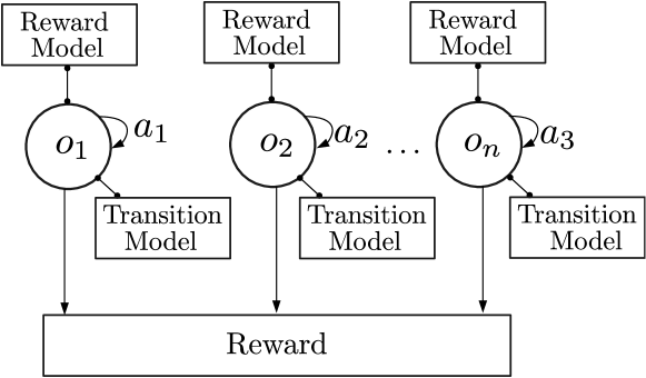
Following the requirements of a plug and play approach, as the first step, we eliminate the need for a single agent to adjust all objects. Instead, independent objects inherit attributes from their class and maintain their own local transition model and reward model. The global transition dynamics is represented as a union of local transition models, each with respect to one class of active objects in the scene. Transition dynamics from an object class are pre-learnt and ready for use in a new environment. Scenes can also be dynamically configured with addition and removal of objects, and number of objects can be arbitrarily large as they do not share a common reward model or a transition model. Additionally, we develop a novel ‘trust factor’ based transfer mechanism for reward functions across environments. We term our approach as Plug and Play Reinforcement Learning (PaPRL). Figure 1 shows the overall structure of a plug and play approach.

Experiments show that our representation achieves sample-efficiency in a variety of set-ups from simple to complex environments. Building upon the plug and play environments, objects can be arbitrarily added or removed during the run time. To illustrate the effects of local transition model of a class of objects, we consider two cases of (1) learning the local transition models in an inexpensive and fast simulator and then transfer/plug in a new environment (PaPRL-offline), and (2) learning local transition model for each object during the run time (PaPRL-online).

2 Related Works

Figure 1: A Plug and play environment in which objects inherit a reward model and a transition model form their class.

This work builds upon three areas of related research:

Physics-Based Reinforcement Learning: In physics based reinforcement learning, Deep Lagrangian Networks Lutter et al. (2019) and Interaction Networks Battaglia et al. (2016) aim to reason about the way objects in complex systems interact. Deep Lagrangian Networks (DeLaN) Lutter et al. (2019) encode the physics prior in the form of a differential in the network topology to achieve lower sample complexity and better extrapolation. However, these works use a global transition model. Whilst they can naturally handle arbitrary number of objects, they are not flexible in including new classes of objects. Consequently, new class of objects require complete retraining of the global transition model, and hence, this may not be feasible in a plug and play setting in which the new classes of objects may be introduced at any time.

Object-Oriented Reinforcement Learning: Object-oriented MDPs Diuk et al. (2008) are an extension to the standard MDPs to construct the global transition dynamics of the environment and develop an object-oriented non-transferable reinforcement learning. Following this approach some studies address the need for object-centric understanding of the environment Cobo et al. (2013); Garnelo et al. (2016); Keramati et al. (2018), however, they are not naturally transferable to a new scene as the objects’ properties cannot be reused in a new environment. Keramati et al. Keramati et al. (2018) aims to boost the performance of agents in a large state space with sparse reward. Schema networks Kansky et al. (2017) use a vision system that detects and tracks entities in an image. Given the entities, a self-transition variable is defined to represent the probability that a position attribute remains active in the next time step. While this self-transition variable can be sufficient in some video games, it may not be suitable for more complex physical environments with many attributes for objects. Scholz et al. Scholz et al. (2014) propose a A Physics-Based model prior for object-oriented Reinforcement Learning (PBLR) with a focus on Robotics applications. This representation defined a state-space dynamics function in terms of the agent’s beliefs over objects’ inertial parameters and the existence and parametrisation of physical constraints. PBLR’s approach is quite different and the solutions do not translate into the settings of a Plug and Play framework in which every object holds its own inherited properties. Model-based reinforcement learning approaches such as COBRA Watters et al. (2019) aim to learn representations of the world in terms of objects and their interactions and pass this knowledge as a transition model to the single agent and with a global reward model. Hence, this approach cannot be used in a plug and play environment in which the objects are acting based on their own local transition model and their own reward model.

Multi-Agent Reinforcement Learning: These approaches may also be considered as related studies as in our proposed method, objects can perform actions in the environment. However, the focus of multi-agent methods is generally on improving the cooperation setting among agents with same class of attributes to maximise a common long-term return, and thus are not suitable for a plug and play environment where objects can come from a variety of classes. MOO-MDP Da Silva et al. (2017) is a study that combines the concept of object-oriented representation and multi-agent reinforcement learning. This method is a model-free algorithm but uses a global transition model to solve deterministic multi-agent, object-oriented problems with a discrete action. The extracted knowledge from objects are not transferable to a new environment. Model-based multi-Agent reinforcement learning approaches such as Bargiacchi et al. (2020), aim to learn a model of the environment and update a single reward model in a sample-efficient manner with cooperation among agents. We however, are interested in modelling local transition dynamics, and we consider the agents to act independently.

Relations to Plug and Play Environments: Based on the three main requirements of a plug and play environment, physics-based reinforcement learning approaches fail to fit into this setting as they only develop a global transition model of the environment. Whilst some of the object-oriented reinforcement learning approaches construct local transition models, but they develop a single reward model that is incompatible with the plug and play approach. Additionally, local transition models of objects in such methods are not reusable in new environments as they are environment-specific. Model-based multi-agent reinforcement learning methods generally work with similar agents with same classes of attributes and the focus of such methods is on improving the co-operation of agents with the help of global transition model to achieve the highest return. Consequently, such approaches cannot be applied into a plug and play environment.

3 Plug and Play Markov Decision Processes

Following the sequential decision-making problems, our plug and play reinforcement learning framework is constructed based on MDPs and object oriented MDPs. Plug and Play Markov Decision Process (PaP-MDP) is described by $<\mathcal{\mathrm{{\mathcal{O}},\ }{C}},\mathcal{Z},\mathcal{{A}},\mathcal{{P}},\mathcal{{R}}>$, where:

• $\mathcal{{O}}=\{o_{1},o_{2},\ldots,o_{O}\}$ is the set of objects that are existing in the environment,

• $\mathcal{{C}=}\{c_{1},c_{2},\ldots,c_{C}\}$ is the set of classes of objects that are present in the environment,

• $\mathcal{Z}=\{z_{1},z_{2},\ldots,z_{O}\}$ is the set of booleans that determines if an object is allowed to take an action in the environment: $z_{i}=\{0,1\},\mathrm{and}\sum_{i\in\{1,\ldots,O\}}z_{i}=O^{\prime};1\leq O^{\prime}\leq O$,

• $\mathcal{{A}}=\{a_{1},a_{2},\ldots,a_{O}\}$ is the set of valid actions the objects in the environment $o_{i}\in\mathcal{O}$ may take at every time-step if $z_{i}=1$,

• $\mathcal{{P}}=\{p_{1},p{}_{2},\ldots,p_{O}\}$ is the set of local transition models for the objects in the environment $o_{i}\in\mathcal{O}$ if $z_{i}=1$; and

• $\mathcal{{R}}$ is the global reward function.

Different classes of objects have distinct attributes: $\mathrm{{att}}(c_{i})=\{e_{1}^{i},\ldots,e_{E_{i}}^{i}\},\forall i\in{1,\ldots C}$ and $E_{i}$ is the number of attributes for class $c_{i}$. These attributes are inherited by new objects generated from class $c_{i}$. To efficiently determine the class of each object, we define $\mathrm{C}(o_{i})=c_{k\in\{1\ldots C\}}$ that returns the class of an object. Attributes of objects may be changed only by that specific object. If $z_{i}=1$, then $o_{i}$ can perform an action, we term these objects as active objects. On the other hand, if $z_{i}=0$, then $o_{i}$ is not permitted to perform any action in the environment and we term these objects as neutral objects $\mathcal{N}=\cup o_{i},(\forall i\in\{1,\dots,O\}\land z_{i}=0)$ and $a_{i}=\emptyset$, a null action. Active objects can observe the neutral objects’ attributes. However, active objects are unaware of each others’ attributes and they do not interact directly with each other.

Given the definition of objects and attributes, the state of an object $o_{i}$ in the environment is defined as:

$$o_{i}.s=[o_{i}.e_{1}^{\mathrm{C}(o_{i})},\ldots,o_{i}.e_{E}^{\mathrm{C}(o_{i})}]$$ (1)

where the the “dot” notation denotes the attribute of an object. The state of PaP-MDP is defined as the union of all states for different objects that are present in the environment:

$$\mathcal{S}=\cup_{\forall o\in\mathcal{{O}}}\quad o.s$$ (2)

3.1 Local Transition Models

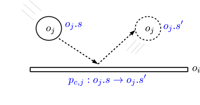
Local transition models are defined for each class of active objects in the environment. These local models act as dynamics models that learn and encode the behaviour of different classes of active objects as they interact with neutral objects. $p_{c,j}:o_{j}.s\rightarrow o_{j}.s^{\prime},\forall o_{j}\in\mathcal{N}$, is an approximation of a local transition function for active object $o_{i},c=\mathrm{C}(o_{i})$, that learns how to predict the next state of the neutral object $o_{j}$ in the environment after they interact. Active objects can observe the attributes of neutral objects, hence, they can simply record the attributes of the neutral object before and after the interaction, e.g. a collision can be determined based on the distance of the objects. As an example, Figure 2 shows an active object $o_{i}$ before and after collision with a neutral object $o_{j}$. $p_{c,j},c=\mathrm{C}(o_{i})$, the local transition model, predicts $o_{j}.s^{\prime}$ given $o_{j}.s$ - that is the state of the neutral object before the collision with $o_{i}$. Linear function approximation may suffice to describe simple interactions, for more complex and non-linear behaviours such as collision, a non-linear function approximator is required. In this case, we use a neural network $\mathcal{D}$ with weights $\theta$ trained with a backpropagation algorithm to learn the interaction in a supervised manner. The network is trained to minimise the MSE loss, using the post-interaction state of the neutral object $o_{j}$ as label:

$$\mathcal{L}_{j}(\theta)=\mathrm{\mathbb{E}}[(o_{j}.s^{\prime}-\mathcal{D}(o_{j}.s,\theta))^{2}]$$

The active objects thus predict the post-interaction state of the neutral object before interaction.

Figure 2: The interaction between $o_{i}$ and neutral object $o_{j}$ is modeled by $p_{c,j}$.

3.2 Reward Learning Algorithm

Following PHYRE study Bakhtin et al. (2019), we design our main experimental environment to be “wait and see”. Each active object ($\forall o_{i}\notin\mathcal{N}$) is allowed to perform an action only if interacting with a neutral object $o_{j}$. If $o_{i}$ and $o_{j}$ interact more than one time during an episode, $o_{i}$ is not allowed to perform more actions and will be treated as a neutral object until it receives the reward and completes the episode.

3.2.1 Reward Model

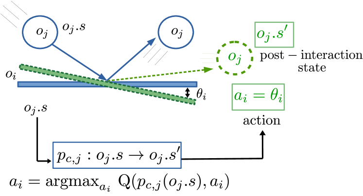
We use a specific type of DQN to model the reward function in the environment. Note that in the proposed problem, objects cannot perform more than one action in a single episode and the time-steps are eliminated. As a result, the Q-network of an active object represents a model of its reward function. All active objects have one common goal, yet they are not aware of each other’s attributes. Given that, each object collects a set of state-action-reward triplets after interacting with a neutral object. However, given the trained local transition model for each active object, we use triplets of the form “¡post-interaction state, action, reward¿’’. We argue that the learned local transition model is a critical prior knowledge about the physics of an object that can improve sample-efficiency of this approach. In a practical sense, an active object can adjust itself by performing an action that results in a post-interaction state which is more favourable to achieve the highest reward. Consider the example of a ball as a neutral object ($o_{j}\in\mathcal{N}$) and an obstacle ($o_{i}\notin\mathcal{N}$) as an active object. Given the collision as a type of interaction we are interested in, Figure 3 shows that given $p_{c,j},c=\mathrm{C}(o_{i})$, the local transition model, $o_{i}$ performs an action which results in desirable post-interaction state that is expected to return the highest global reward:

$$a_{i}=\mathrm{argmax}_{a}o_{i}\mathrm{.Q}(p_{c,j}(o_{j}.s),a_{i}),\quad c=\mathrm{C}(o_{i})$$ (3)

where $\mathrm{Q}$ is a neural network that is minimised by MSE loss between the prediction and the observed reward:

$$\mathcal{L^{\prime}}_{j}(\theta)=\mathrm{E}[(r(\mathcal{S},\mathcal{A})-o_{i}.\mathrm{Q}(p_{c,j}(o_{j}.s),a_{i}))^{2}],\quad c=\mathrm{C}(o_{i}).$$ (4)

Note that $r(\mathcal{S},\mathcal{A})$ is the global reward function based on the environment’s set of states $\mathcal{S}$ and object’s set of actions $\mathcal{A}$.

Figure 3: An example of interaction between active object $o_{i}$ and neutral object $o_{j}$. As $o_{i}$ observes the attributes of $o_{j}$, it performs a rotation action $a_{i}$ that results in the post-interaction state $o_{j}.s^{\prime}$ that is the most favourable to return the highest reward based on the trained rewarding model. Solid blue arrows show the trajectory of $o_{j}$ if no action is taken by $o_{i}$. Green dashed arrows shows the post-interaction trajectory of $o_{j}$ if action $a_{i}$ is performed.

3.2.2 Trust Factor

A key part of our plug and play reinforcement learning framework is derived from the concept of object oriented environments. As demonstrated in reward learning section, each active object $o_{i}\notin\mathcal{N}$ constructs its own reward model $o_{i}\mathrm{.Q}$. However, $o_{i}$ also inherits a reward function from class $\mathrm{C}(o_{i})$ upon initilisation, as the reward model is also one of the attributes of that class. We term an inherited reward model for $o_{i}$ from class $c=\mathrm{C}(o_{i})$, as $c.\mathrm{Q}.$ The inherited reward model may not be the best choice as a new active object can be initialised with different attributes such as position, length, weight, etc. We impose no restrictions on $c.\mathrm{Q}$ and it can be a randomly initialised neural network or any reward model from one of the previously trained objects from that class. If the class reward model is selected from one of the previously trained objects in the environment, a newly initialised object may find the class reward function as a reasonable starting model to partially rely on. To leverage the mixed use of class and object models, we define a trust factor that intuitively measures how accurately a reward model for an active object works. The trust factor of approximated reward function $\mathrm{Q}$ at iteration $t$ as:

$$\mathrm{TF}_{t}(\mathrm{Q})=(1+\sum_{k=1}^{K}|r(\mathcal{S},\mathcal{A})-\mathrm{Q}(p_{c,j}(o_{j}.s),a_{i})|)^{-1},\enskip c=\mathrm{C}(o_{i})$$ (5)

where $K$ is the number of episodes an object waits to calculate its trust to the current reward model $\mathrm{Q}\in\{o_{i}.\mathrm{Q},\mathrm{C}(o_{i}).\mathrm{Q}\}$ that is currently being used. If the difference of the predicted and the actual received rewards is considerable, the trust factor will be low and the object attempts to use the alternative reward function for the next round. Algorithm 1 shows the trust factor calculation.

Algorithm 1 Trust Factor Calculation for Active Objects

1:  Input:

2:  Active objects present in the environment: $\forall o_{i}\notin\mathcal{N}$,

3:  Neutral objects present in the environment: $\forall o_{j}\in\mathcal{N}$,

4:  Reward models for all active objects $\mathrm{Q}\in\{o_{i}.\mathrm{Q},\mathrm{C}(o_{i}).\mathrm{Q}\},o_{i}\notin\mathcal{N}$,

5:  Initialize $K$, the step size and the trust threshold $h$ (see 5).

6:  Output: Trust factors for all active objects at episode $t$: $\mathrm{TF}_{t}(\mathrm{Q})$.

7:  for $\forall o_{i}$ do

8:     $\mathrm{TF}_{t}(\mathrm{Q})=(1+\sum_{k=1}^{K}|r(\mathcal{S},\mathcal{A})-\mathrm{\mathrm{Q}}(p_{c,j}(o_{j}.s),a_{i})|)^{-1}$

9:     if $\mathrm{TF}_{t}(\mathrm{Q})\leq h$ then

10:        $\mathrm{\mathrm{Q}=Replace}(o_{i}.\mathrm{Q},\mathrm{C}(o_{i}).\mathrm{Q})\quad$//Replace the current reward model with the other available reward model

11:     end if

12:  end for

Figure 4: Plug and Play Reinforcement Learning

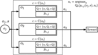
Figure 4 shows the overview of our proposed plug and play reinforcement learning framework in which all the objects inherit their class attributes and attempt to maximise their own constructed reward. Algorithm 2 outlines the pseudo code of plug and play reinforcement learning.

Algorithm 2 Plug and Play Reinforcement Learning Algorithm

1:  Input:

2:  Active objects present in the environment: $\forall o_{i}\notin\mathcal{N}$,

3:  Neutral objects present in the environment: $\forall o_{j}\in\mathcal{N}$,

4:  Reward models for all active objects $\mathrm{Q}\in\{o_{i}.\mathrm{Q},\mathrm{C}(o_{i}).\mathrm{Q}\},\forall o_{i}\notin\mathcal{N}$,

5:  Initialize $K$, the step size and the trust threshold $h$ (see 5).

6:  Output: Updated estimates of $\mathrm{Q}\in\{o_{i}.\mathrm{Q},\mathrm{C}(o_{i}).\mathrm{Q}\},\forall o_{i}\notin\mathcal{N}$.

7:  for $\forall o_{j},\ o_{j}\in\mathcal{N}$ do

8:     for $\forall o_{i},\ o_{i}\notin\mathcal{N}$ do

9:        if $\mathrm{interact}(o_{j},o_{i})$ then

10:           $a_{i}=\mathrm{argmax}_{a_{i}}\mathrm{Q}(p_{c,j}(o_{j}.s),a_{i}),\quad c=\mathrm{C}(o_{i})$.

11:           Construct the $<o_{j}.s^{\prime}$, $a_{i}$, $r(\mathcal{S},\mathcal{A})>$ and append to the observation set.

12:           Sample a random minibatch of triplets and update $\mathrm{Q}$ with minimising Loss function 4.

13:           if $\mathrm{TF}_{t}(\mathrm{Q})\leq h$ then

14:              $\mathrm{\mathrm{Q}=Replace}(o_{i}.\mathrm{Q},\mathrm{C}(o_{i}).\mathrm{Q})\quad$ //Replace the current reward (Algorithm 1)

15:           end if

16:        end if

17:     end for

18:  end for

4 Experiments

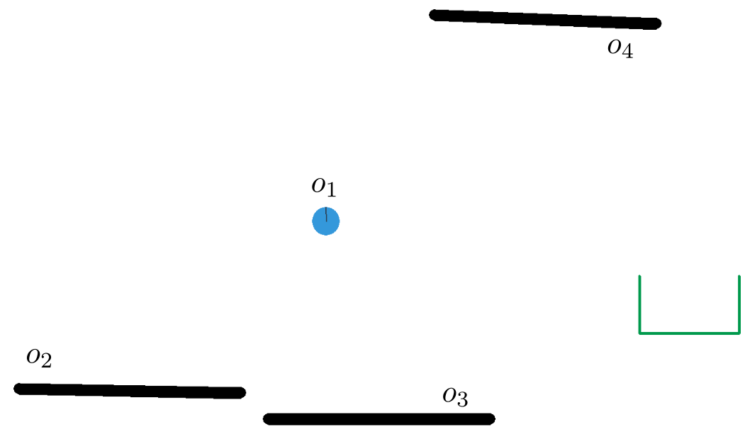
(a) Rotating Wall active objects and the neutral-ball.

(b) Arc Wall active objects (red) and the neutral-ball (blue).

Figure 5: A sample experiment with active and neutral objects $\{o_{1}\}\in\mathcal{N},\{o_{2},o_{3},o_{4}\}\notin\mathcal{N}$. Active objects receive the highest reward if the neutral-ball falls in the green basket.

(a) An environment with $\{o_{1}\}\in\mathcal{N},\{o_{2}\}\notin\mathcal{N}$ as rotating wall.

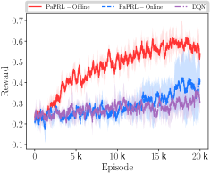
(b) Obtained reward from the environment.

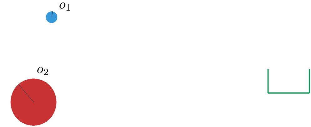
(c) An environment with $\{o_{1}\}\in\mathcal{N},\{o_{2}\}\notin\mathcal{N}$ as the arc wall.

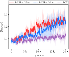
(d) Obtained reward from the environment.

(e) An environment with $\{o_{1}\}\in\mathcal{N},\{o_{2},o_{3}\}\notin\mathcal{N}$ with two rotating walls.

(f) Obtained reward from the environment.

(g) An environment with $\{o_{1}\}\in\mathcal{N},\{o_{2},o_{3}\}\notin\mathcal{N}$ as arc walls.

(h) Obtained reward from the environment.

Figure 6: Single (first row) and many (second row) active objects (rotating wall and arc wall) in the environment with a comparison of PaP-RL and DQN.

In this section, we demonstrate the performance of PaP-RL in a simple plug and play reinforcement learning platform, following which, we present detailed empirical comparisons against the baselines.

4.1 Experimental Setting

In our experiments, we introduce two types of objects: active objects ( Rotating Wall and Arc Wall) that can perform actions, and a neutral object (Neutral-ball) that cannot. The two classes of active objects have their own attributes that can be adjusted by performing the required action to maximise the expected return.

4.1.1 Rotating Wall

The rotating wall class of active objects are constructed by the following attributes:

$$\mathrm{att}(C_{w})=[f_{w},e_{w},\theta_{w}],$$

where $f_{w}\in[0.4,0.9]$ is the friction coefficient of the wall , $e_{w}\in[0.4,0.9]$ is the elasticity coefficient of the wall, and $\theta_{w}\in[-\frac{\pi}{10},\frac{\pi}{10}]$ is the degree of rotation for the wall.

4.1.2 Arc Wall

The arc wall class of active objects are designed by the following attributes:

$$\mathrm{att}(C_{a})=[f_{a},e_{a},\dot{v}_{a}],$$

where $f_{a}\in[0.4,0.9]$ is the friction coefficient of the wall, $e_{a}\in[0.4,0.9]$ is the elasticity coefficient of the wall, and $\dot{v}_{a}\in[-50,50]$ is the angular velocity of the arc wall.

4.1.3 Neutral-ball

We assume the Neutral-ball class of objects have the following attributes:

$$\mathrm{att}(C_{b})=[v_{x},v_{y},\dot{v_{b}},\theta_{b},f_{b},e_{b},m_{b}],$$

where $v_{x}$: velocity in x-axis, $v_{y}$: the velocity in y-axis, $\dot{v_{b}}$: the angular velocity, $\theta_{b}$: the angle of movement, $f_{b}\in[0.4,0.9]$: friction coefficient of the ball, $e_{b}\in[0.4,0.9]$ elasticity coefficient of the ball, and $m_{b}\in[5,25]$: mass of the ball. As discussed before, the post-interaction state of the ball as a neutral object needs to be recorded in order to train the local transition models of each active object. Hence, $o_{j}.s^{\prime}$ can be defined as:

$$o_{j}.s^{\prime}=[v_{x}^{\prime},v_{y}^{\prime},\dot{v}_{b}^{\prime},\theta_{b}^{\prime}],$$

where $v_{x}^{\prime}$: velocity in x-axis after interaction, $v_{y}^{\prime}$: the velocity in y-axis after interaction, $\dot{v}_{b}^{\prime}$: the angular velocity after interaction, $\theta_{b}^{\prime}$: the angle of movement after interaction.

4.1.4 Basket-Ball Platform

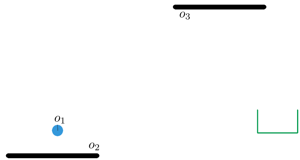
We design a simple platform with one neutral object (blue ball) and several active objects (either rotating or arc walls). The active objects can perform actions to allow the blue ball to reach the basket. A smooth reward function returns the maximum reward if the neutral-ball moves into the desired location (e.g. a Basket). The active object $o_{i}$ receives a reward after interaction with neutral object $o_{j}$ as follows:

$$r(o_{j}.s^{\prime},a_{i})=\begin{cases}1,&\text{if}\ o_{j}\ \mathrm{in\ Basket}\\ {}[\mathcal{\mathrm{Min}}(d)]^{-1},&\text{otherwise}\end{cases}$$ (6)

where $d$ is the distance of the ball with the center of the basket at each time-frame, $o_{j}.s^{\prime}$ is the post-interaction state of $o_{j}$, and $a_{i}$ is the action taken by $o_{i}$ to adjust its attributes. Figure 5 illustrates an example of this platform with two different classes of active objects. At every episode of the environment, a neutral object is generated in a random position and the active objects are required to adjust their attributes by performing the proper action. Note that every active object is only allowed to perform a single action in an episode and wait until it receives the global reward from the environment. Further implementation details with more experiments are available in supplementary materials.

Figure 7: Effects of adding/removing active objects (red arc walls) on the reward for PaPRL and MO-DQN.

4.2 Single Active Object

We start with an environment with a single active object and we proceed to more complex environments. Our first experiment is based on a rotating wall active object and a neutral-ball object.

4.2.1 Baselines

To compare our proposed method with other related approaches, we show the results of following approaches:

• DQN as implemented in PHYRE Bakhtin et al. (2019): For this baseline, we construct the Q-network with state-action pairs and the returned reward as the target. The state in this case, is the state of the neutral objects $o_{j}.s$ that is about to interact with an active object $o_{i}$ that takes an action $a_{i}$ which is expected to result in the highest return. Similar to PHYRE framework that deals with continuous action space, we sample $10,000$ actions at each episode and choose the one with the highest expected reward.

• PaP-Online: PaP-RL with no pre-trained local transition function, hence it learns the local transition models during the run time by observing prior- and post-interaction states.

• PaP-Offline: PaP-RL with pre-trained local transition function from an inexpensive and fast simulator with no reward.

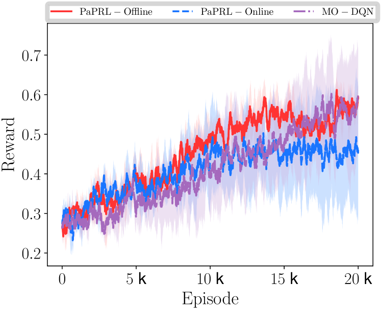
Figure 6 (first row) shows the results of single active object experiments. Our offline and online PaP-RL methods outperforms DQN, with the offline version being more sample-efficient as it relies on a pre-trained local transition model. Whereas, the DQN approach that only relies on prior-interaction of the neutral object and does not benefit from local transition models have a slower rate of improvement.

4.3 Many Active Objects

We now extend the problem to incorporate many active objects $o_{i}\notin\mathcal{N}$ in the environment.

4.3.1 Baselines

To compare our proposed method with other related approaches, we are using two baselines as follows:

• MO-DQN in PHYRE Bakhtin et al. (2019): We extended the implemented DQN for every active object in the environment and we call it Multi-Object DQN (MO-DQN). Following this approach, all the active objects in the environment independently maintain a Q-network based on state-action pairs and the returned reward as explained in the settings of the experiments. Hence, at every episode, $o_{i}$ selects the action that maximises the expected reward based on its constructed reward model.

• PaP-Online: Similar to Single Active Object experiments, we use PaP-RL with no pre-trained local transition function, hence every active object in the environment learns the localy transition models by observing prior- and post-interaction states, and its own reward model independently.

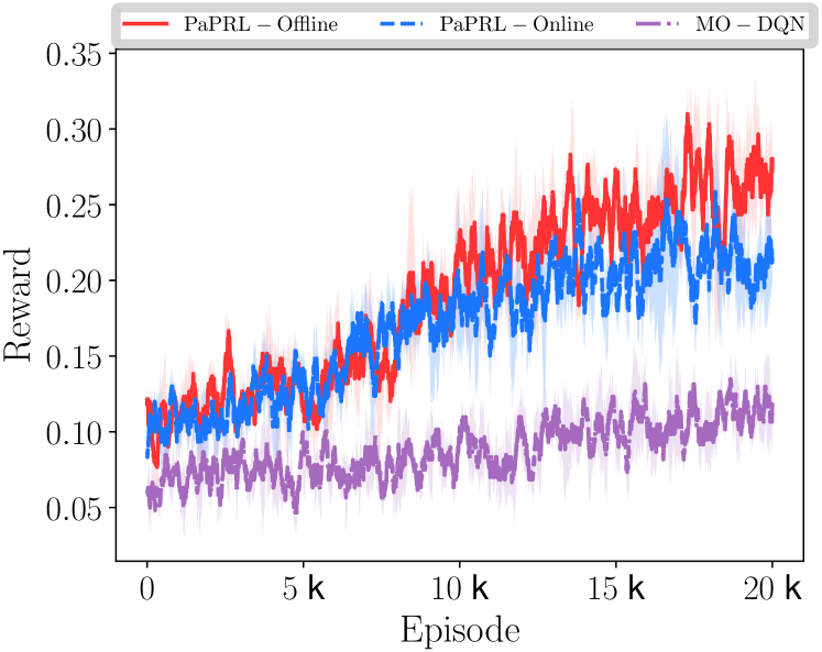
Figure 6 (second row) shows the results of our experiment with many active objects in the environment and it confirm that PaP-RL outperforms DQN with higher numbers of active objects in the environment, with the offline version being better as expected.

4.4 Adding/Removing Objects

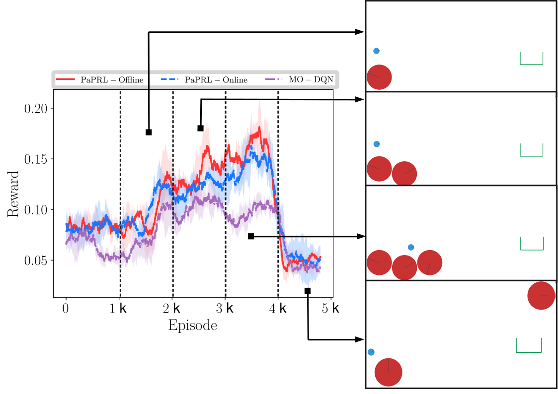
As we have explained before, PaP-MDP is defined to incorporate addition/removal of active objects in the environment. Figure 7 shows the effects of adding/removing objects in the environment during the run time. We compare PaPRL with MO-DQN method by adding new objects after 1000, 2000, and 3000 episodes. To illustrate the effects of removal, two objects are removed at the 4000th episode. Figure 7 shows that both PaPRL and DQN experience a higher rate of improvement when a new object is added to the environment (with an exception of DQN after episode 3000). The reason for this boost of improvement is that the newly added active objects are likely to prevent the neutral ball to leave the environment by violating the environment boundaries and receiving a low reward. Hence, the neutral ball is given more chances for (possible) interactions with new active objects to fall in the basket. Figure 7 also shows that PaPRL-offline outperforms other baselines as it uses the pre-trained local transition models.

5 Conclusion

In this paper, we proposed the Plug and Play Markov Decision Processes to introduce a plug and play, object-centric reinforcement learning approach. In our proposed plug and play approach, independent objects inherit attributes from their class and maintain their own local transition model and reward model. Accordingly, the global transition dynamics is represented as a union of local transition models, each with respect to one class of active objects in the scene. We also showed that in this framework, scenes can also be dynamically configured with addition and removal of objects, and number of objects can be arbitrarily large. Our experimental results prove sample-efficiency of our approach compared to other related methods.

References

- Bakhtin et al. (2019) Bakhtin, A., van der Maaten, L., Johnson, J., Gustafson, L., and Girshick, R. Phyre: A new benchmark for physical reasoning. Advances in Neural Information Processing Systems, 32:5082–5093, 2019.
- Bargiacchi et al. (2020) Bargiacchi, E., Verstraeten, T., Roijers, D. M., and Nowé, A. Model-based multi-agent reinforcement learning with cooperative prioritized sweeping. arXiv preprint arXiv:2001.07527, 2020.
- Battaglia et al. (2016) Battaglia, P., Pascanu, R., Lai, M., Rezende, D. J., et al. Interaction networks for learning about objects, relations and physics. In Advances in neural information processing systems, pp. 4502–4510, 2016.
- Cobo et al. (2013) Cobo, L. C., Isbell Jr, C. L., and Thomaz, A. L. Object focused q-learning for autonomous agents. Georgia Institute of Technology, 2013.
- Da Silva et al. (2017) Da Silva, F. L., Glatt, R., and Costa, A. H. R. Moo-mdp: an object-oriented representation for cooperative multiagent reinforcement learning. IEEE transactions on cybernetics, 49(2):567–579, 2017.
- Diuk et al. (2008) Diuk, C., Cohen, A., and Littman, M. L. An object-oriented representation for efficient reinforcement learning. In Proceedings of the 25th international conference on Machine learning, pp. 240–247, 2008.
- Garnelo et al. (2016) Garnelo, M., Arulkumaran, K., and Shanahan, M. Towards deep symbolic reinforcement learning. arXiv preprint arXiv:1609.05518, 2016.
- Kansky et al. (2017) Kansky, K., Silver, T., Mély, D. A., Eldawy, M., Lázaro-Gredilla, M., Lou, X., Dorfman, N., Sidor, S., Phoenix, S., and George, D. Schema networks: Zero-shot transfer with a generative causal model of intuitive physics. arXiv preprint arXiv:1706.04317, 2017.
- Keramati et al. (2018) Keramati, R., Whang, J., Cho, P., and Brunskill, E. Strategic object oriented reinforcement learning. arXiv preprint arXiv:1806.00175, 2018.
- Lutter et al. (2019) Lutter, M., Ritter, C., and Peters, J. Deep lagrangian networks: Using physics as model prior for deep learning. arXiv preprint arXiv:1907.04490, 2019.
- Scholz et al. (2014) Scholz, J., Levihn, M., Isbell, C., and Wingate, D. A physics-based model prior for object-oriented mdps. In International Conference on Machine Learning, pp. 1089–1097, 2014.
- Van Merriënboer et al. (2015) Van Merriënboer, B., Bahdanau, D., Dumoulin, V., Serdyuk, D., Warde-Farley, D., Chorowski, J., and Bengio, Y. Blocks and fuel: Frameworks for deep learning. arXiv preprint arXiv:1506.00619, 2015.
- Watters et al. (2019) Watters, N., Matthey, L., Bosnjak, M., Burgess, C. P., and Lerchner, A. Cobra: Data-efficient model-based rl through unsupervised object discovery and curiosity-driven exploration. arXiv preprint arXiv:1905.09275, 2019.