Distributed Transformations of Hamiltonian Shapes based on Line Moves

Abstract

We consider a discrete system of $n$ simple indistinguishable devices, called agents, forming a connected shape $S_{I}$ on a two-dimensional square grid. Agents are equipped with a linear-strength mechanism, called a line move, by which an agent can push a whole line of consecutive agents in one of the four directions in a single time-step. We study the problem of transforming an initial shape $S_{I}$ into a given target shape $S_{F}$ via a finite sequence of line moves in a distributed model, where each agent can observe the states of nearby agents in a Moore neighbourhood. Our main contribution is the first distributed connectivity-preserving transformation that exploits line moves within a total of $O(n\log_{2}n)$ moves, which is asymptotically equivalent to that of the best-known centralised transformations. The algorithm solves the line formation problem that allows agents to form a final straight line $S_{L}$, starting from any shape $S_{I}$, whose associated graph contains a Hamiltonian path.

1 Introduction

The explosive growth of advanced technology over the last few decades has contributed significantly towards the development of a wide variety of distributed systems consisting of large collections of tiny robotic-units, known as monads. These monads are able to move and communicate with each other by being equipped with microcontrollers, actuators and sensors. However, each monad is severely restricted and has limited computational capabilities, such as a constant memory and lack of global knowledge. Further, monads are typically homogeneous, anonymous and indistinguishable from each other. Through a simple set of rules and local actions, they collectively act as a single unit and carry out several complex tasks, such as transformations and explorations.

In this context, scientists from different disciplines have made great efforts towards developing innovative, scalable and adaptive collective robotic systems. This vision has recently given rise to the area of programmable matter, first proposed by Toffoli and Margolus [36] in 1991, referring to any kind of materials that can algorithmically change their physical properties, such as shape, colour, density and conductivity through transformations executed by an underlying program. This newborn area has been of growing interest lately both from a theoretical and a practical viewpoint.

One can categorise programmable matter systems into active and passive. Entities in the passive systems have no control over their movements. Instead, they move via interactions with the environment based on their own structural characteristics. Prominent examples of research on passive systems appear in the areas of population protocols [7, 28, 29], DNA computing [1, 8] and tile self-assembly [15, 34, 38]. On the other hand, the active systems allow computational entities to act and control their movements in order to accomplish a given task, which is our primary focus in this work. The most popular examples of active systems include metamorphic systems [19, 31, 37], swarm/mobile robotics [10, 21, 32, 35, 40], modular self-reconfigurable robotics [5, 22, 41] and recent research on programmable matter [12, 13]. Moreover, those robotic systems have received an increasing attention from the the engineering research community, and hence many solutions and frameworks have been produced for milli/micro-scale [9, 23, 26] down to nanoscale systems [16, 33].

Shape transformations (sometimes called pattern formation) can be seen as one of the most essential goals for almost every system among the vast variety of robotic systems including programmable matter and swarm robotic systems. In this work, we focus on a system of a two-dimensional square grid containing a collection of entities typically connected to each other and forming an initial connected shape $S_{I}$. Each entity is equipped with a linear-strength mechanism that can push an entire line of consecutive entities one position in a single time-step in a given direction of a grid. The goal is to design an algorithm that can transform an initial shape $S_{I}$ into a given target shape $S_{F}$ through a chain of permissible moves and without losing the connectivity. That is, in each intermediate configuration we always want to guarantee that the graphs induced by the nodes occupied by the entities are connected. The connectivity-preservation is an important assumption for many practical applications, which usually require energy for data exchange as well as the implementation of various locomotion mechanisms.

1.1 Related Work

Many models of centralised or distributed coordination have been studied in the context of shape transformation problems. The assumed mechanisms in those models can significantly influence the efficiency and feasibility of shape transformations. For example, the authors of [2, 17, 18, 19, 27] consider mechanisms called sliding and rotation by which an agent can move and turn over neighbours through empty space. Under these models of individual movements, Dumitrescu and Pach [17] and Michail et al. [27] present universal transformations for any pair of connected shapes $(S_{I},S_{F})$ of the same size to each other. By restricting to rotation only, the authors in [27] proved that the decision problem of transformability is in $\mathbf{P}$; however, with a constant number of extra seed nodes connectivity preserving transformation can be completed with $\Omega(n^{2})$ moves [27].

The alternative less costly reconfiguration solutions can be designed by employing some parallelism,where multiple movements can occur at the same time, see theoretical studies in [11, 14] and more practical implementation in [35]. Moreover, it has been shown that there exists a universal transformation with rotation and sliding that converts any pair of connected shapes to each other within $O(n)$ parallel moves in the worst case [27]. Also fast reconfiguration might be achieved by exploiting actuation mechanisms, where a single agent is now equipped with more strength to move many entities in parallel in a single time-step. A prominent example is the linear-strength model of Aloupis et al. [5, 6], where an entity is equipped with arms giving it the ability to extend/extract a neighbour, a set of individuals or the whole configuration in a single operation. Another elegant approach by Woods et al. [39] studied another linear-strength mechanism by which an entity can drag a chain of entities parallel to one of the axes directions.

A more recent study along this direction is shown in [4], and introduces the line-pushing model. In this model, an individual entity can push the whole line of consecutive entities one position in a given direction in a single time-step. As we shall explain, this model generalises some existing constant-strength models with a special focus on exploiting its parallel power for fast and more general transformations. Apart from the purely theoretical benefit of exploring fast reconfigurations, this model also provides a practical framework for more efficient reconfigurations in real systems. For example, self-organising robots could be reconfiguring into multiple shapes in order to pass through canals, bridges or corridors in a mine. In another domain, individual robots could be containers equipped with motors that can push an entire row to manage space in large warehouses. Another future application could be a system of very tiny particles injected into a human body and transforming into several shapes in order to efficiently traverse through the veins and capillaries and treat infected cells.

This model is capable of simulating some constant-strength models. For example, it can simulate the sliding and rotation model [17, 27] with an increase in the worst-case running time only by a factor of 2. This implies that all universality and reversibility properties of individual-move transformations still hold true in this model. Also, the model allows the diagonal connections on the grid. Several sub-quadratic time centralised transformations have been proposed, including an $O(n\sqrt{n})$-time universal transformation that preserves the connectivity of the shape during its course [3]. By allowing transformations to disconnect the shape during their course, there exists a centralised universal transformation that completes within $O(n\log n)$ time.

Another recent related set of models studied in [10, 20, 24] consider a single robot which moves over a static shape consisting of tiles and the goal is for the robot to transform the shape by carrying one tile at a time. In those systems, the single robot which controls and carries out the transformation is typically modelled as a finite automaton. Those models can be viewed as partially centralised as on one hand they have a unique controller but on the other hand that controller is operating locally and suffering from a lack of global information.

1.2 Our Contribution

In this work, our main objective is to give the first distributed transformations for programmable matter systems implementing the linear-strength mechanism of the model of line moves. All existing transformations for this model are centralised, thus, even though they reveal the underlying transformation complexities, they are not directly applicable to real programmable matter systems. Our goal is to develop distributed transformations that, if possible, will preserve all the good properties of the corresponding centralised solutions. These include the move complexity (i.e., the total number of line moves) of the transformations and their ability to preserve the connectivity of the shape throughout their course.

However, there are considerable technical challenges that one must deal with in order to develop such a distributed solution. As will become evident, the lack of global knowledge of the individual entities and the condition of preserving connectivity greatly complicate the transformation, even when restricted to special families of shapes. Timing is an essential issue as the line needs to know when to start/stop pushing. When moving or turning, all agents of the line must follow the same route, ensuring that no one is being pushed off. There is an additional difficulty due to the fact that agents do not automatically know whether they have been pushed (but it might be possible to infer this through communication and/or local observation).

Consider a discrete system of $n$ simple indistinguishable devices, called agents, forming a connected shape $S_{I}$ on a two-dimensional square grid. Agents act as finite-state automata (i.e., they have constant memory) that can observe the states of nearby agents in a Moore neighbourhood (i.e., the eight cells surrounding an agent on the square gird). They operate in synchronised Look-Compute-Move (LCM) cycles on the grid. All communication is local, and actuation is based on this local information as well as the agent’s internal state.

Let us consider a very simple distributed transformation of a diagonal line shape $S_{D}$ into a straight line $S_{L}$, $|S_{D}|=|S_{L}|=n$, in which all agents execute the same procedure in parallel synchronous rounds. In general, the diagonal appears to be a hard instance because any parallelism related to line moves that might potentially be exploited does not come for free. Initially, all agents are occupying the consecutive diagonal cells on the grid $(x_{1},y_{1}),(x_{1}+1,y_{1}+1),\ldots,(x_{1}+n-1,y_{1}+n-1)$. In each round, an agent $p_{i}=(x,y)$ moves one step down if $(x-1,y-1)$ is occupied, otherwise it stays still in its current cell. After $O(n)$ rounds, all agents form $S_{L}$ within a total number of $1+2+\ldots+n=O(n^{2})$ moves, while preserving connectivity during the transformation (throughout, connectivity includes horizontal, vertical, and diagonal adjacency). See Figure 1.

Figure 1: A simulation of the simple procedure. From left to right, rounds $0,1,2,\ldots,n$.

The above transformation, even though time-optimal has a move complexity asymptotically equal to the worst-case single-move distance between $S_{I}$ and $S_{F}$. This is because it always moves individual agents, thus not exploiting the inherent parallelism of line moves. Our goal, is to trade time for number of line moves in order to develop alternative distributed transformations which will complete within a sub-quadratic number of moves. Given that actuation is a major source of energy consumption in real programmable matter and robotic systems, moves minimisation is expected to contribute in the deployment and implementation of energy-efficient systems.

We already know that there is a centralised $O(n\log n)$-move connectivity-preserving transformation, working for a large family of connected shapes [3]. That centralised strategy transforms a pair of connected shapes $(S_{I},S_{F})$ of the same order (i.e., the number of agents) to each other, when the associated graphs of both shapes contain a Hamiltonian path (see also Itai et al. [25] for rectilinear Hamiltonian paths), while preserving connectivity during the transformation. This approach initially forms a line from one endpoint of the Hamiltonian path, then flattens all agents along the path gradually via line moves, while successively doubling the line length in each round. After $O(n\log n)$ moves, it arrives at the final straight line $S_{L}$ of length $n$, which can be then transformed into $S_{F}$ by reversing the transformation of $S_{F}$ into $S_{L}$, within the same asymptotic number of moves.

In this work, we introduce the first distributed transformation exploiting the linear-strength mechanism of the line-pushing model. It provides a solution to the line formation problem, that is, for any initial Hamiltonian shape $S_{I}$, form a final straight line $S_{L}$ of the same order. It is essentially a distributed implementation of the centralised Hamiltonian transformation of [3]. We show that it preserves the asymptotic bound of $O(n\log n)$ line moves (which is still the best-known centralised bound), while keeping the whole shape connected throughout its course. This is the first step towards distributed transformations between any pair of Hamiltonian shapes. The inverse of this transformation ($S_{L}$ into $S_{I}$) appears to be a much more complicated problem to solve as the agents need to somehow know an encoding of the shape to be constructed and that in contrast to the centralised case, reversibility does not apply in a straightforward way. Hence, the reverse of this transformation ($S_{L}$ into $S_{I}$) is left as a future research direction.

We restrict attention to the class of Hamiltonian shapes. This class, apart from being a reasonable first step in the direction of distributed transformations in the given setting, might give insight to the future development of universal distributed transformations, i.e., distributed transformations working for any possible pair of initial and target shapes. This is because geometric shapes tend to have long simple paths. For example, the length of their longest path is provably at least $\sqrt{n}$. We here focus on developing efficient distributed transformations for the extreme case in which the longest path is a Hamiltonian path. However, one might be able to apply our Hamiltonian transformation to any pair of shapes, by, for example, running a different or similar transformation along branches of the longest path and then running our transformation on the longest path. We leave how to exploit the longest path in the general case (i.e., when initial and target shapes are not necessarily Hamiltonian) as an interesting open problem.

We assume that a pre-processing phase provides the Hamiltonian path, i.e., a global sense of direction is made available to the agents through a labelling of their local ports (e.g., each agent maintains two local ports incident to its predecessor and successor on the path). Similar assumptions exist in the literature of systems of complex shapes that contain a vast number of self-organising and limited entities. A prominent example is [35] in which the transformation relies on an initial central phase to gain some information about the number of entities in the system.

Now, we are ready to sketch a high-level description of the transformation. A Hamiltonian path $P$ in the initial shape $S_{I}$ starts with a head on one endpoint labelled $l_{h}$, which is leading the process and coordinating all the sub-procedures during the transformation. The transformation proceeds in $\log n$ phases, each consisting of six sub-phases (or sub-routines) and every sub-phase running for one or more synchronous rounds. Figure 2 gives an illustration of a phase of this transformation when applied on the diagonal line shape. Initially, the head $l_{h}$ forms a trivial line of length 1. By the beginning of each phase $i$, $0\leq i\leq\log n-1$, there exists a line $L_{i}$ starting from the head $l_{h}$ and ending at a tail $l_{t}$ with $2^{i}-2$ internal agents labelled $l$ in between. By the end of phase $i$, $L_{i}$ will have doubled its length as follows.

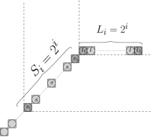
(a) DefineSeg, CheckSeg and DrawMap.

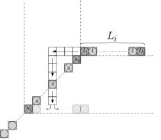
(b) Push.

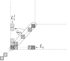
(c) RecursiveCall.

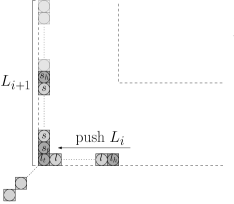
(d) Merge.

Figure 2: From [3], a snapshot of phase $i$ of the Hamiltonian transformation on the shape of a diagonal line. Each occupied cell shows the current label state of an agent. Light grey cells show ending cells of the corresponding moves.

In DrawMap, $l_{h}$ designates a route on the grid through which $L_{i}$ pushes itself towards the tail $s_{t}$ of $S_{i}$. It consists of two primitives: ComputeDistance and CollectArrows. In ComputeDistance, the line agents act as a distributed counter to compute the Manhattan distance between the tails of $L_{i}$ and $S_{i}$. In CollectArrows, the local directions are gathered from $S_{i}$’s agents and distributed into $L_{i}$’s agents, which collectively draw the route map. Once this is done, $L_{i}$ becomes ready to move and $l_{h}$ can start the Push sub-phase. During pushing, $l_{h}$ and $l_{t}$ synchronise the movements of $L_{i}$’s agents as follows: (1) $l_{h}$ pushes while $l_{t}$ is guiding the other line agents through the computed route and (2) both are coordinating any required swapping of states with agents that are not part of $L_{i}$ but reside in $L_{i}$’s trajectory. Once $L_{i}$ has traversed the route completely, $l_{h}$ calls RecursiveCall to apply the general procedure recursively on $S_{i}$ in order to transform it into a line $L_{i}^{\prime}$. Figure 3 shows a graphical illustration of the core recursion on the special case of a diagonal line shape. Finally, the agents of $L_{i}$ and $L_{i}^{\prime}$ combine into a new straight line $L_{i+1}$ of $2^{i+1}$ agents through the Merge sub-procedure. Then, the head $l_{h}$ of $L_{i+1}$ begins a new phase $i+1$.

Figure 3: A zoomed-in picture of the core recursive technique RecursiveCall in Figure 2(c).

Section 2 formally defines the model and the problem under consideration. Section 3 presents our distributed connectivity-preserving transformation that solves the line formation problem for Hamiltonian shapes, achieving a total of $O(n\log n)$ line moves.

2 Model

We consider a system consisting of $n$ agents forming a connected shape $S$ on a two-dimensional square grid in which each agent $p\in S$ occupies a unique cell $cell(p)=(x,y)$, where $x$ indicates columns and $y$ represents rows. Throughout, an agent shall also be referred to by its coordinates. Each cell $(x,y)$ is surrounded by eight adjacent cells in each cardinal and ordinal direction, (N, E, S, W, NE, NW, SE, SW). At any time, a cell $(x,y)$ can be in one of two states, either empty or occupied. An agent $p\in S$ is a neighbour of (or adjacent to) another agent $p^{\prime}\in S$, if $p^{\prime}$ occupies one of the eight adjacent cells surrounding $p$, that is their coordinates satisfy $p^{\prime}_{x}-1\leq p_{x}\leq p^{\prime}_{x}+1$ and $p^{\prime}_{y}-1\leq p_{y}\leq p^{\prime}_{y}+1$, see Figure 4. For any shape $S$, we associate a graph $G(S)=(V,E)$ defined as follows, where $V$ represents agents of $S$ and $E$ contains all pairs of adjacent neighbours, i.e. $(p,p^{\prime})\in E$ iff $p$ and $p^{\prime}$ are neighbours in $S$. We say that a shape $S$ is connected iff $G(S)$ is a connected graph. The distance between agents $p\in S$ and $p^{\prime}\in S$ is defined as the Manhattan distance between their cells, $\Delta(p,p^{\prime})=|p_{x}-p^{\prime}_{x}|+|p_{y}-p^{\prime}_{y}|$. A shape $S$ is called Hamiltonian shape iff $G(S)$ contains a Hamiltonian path, i.e. a path starting from some $p\in S$, visiting every agent in $S$ and ending at some $p^{\prime}\in S$, where $p\neq p^{\prime}$.

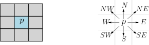
Figure 4: An agent $p$ is a neighbour to any agent locating at one of the eight surrounding cells in grey.

In this work, each agent is equipped with the linear-strength mechanism introduced in [4], called the line pushing mechanism. A line $L$ consists of a sequence of $k$ agents occupying consecutive cells on the grid, say w.l.o.g, $L=(x,y),(x+1,y),\ldots,(x+k-1,y)$, where $1\leq k\leq n$. The agent $p\in L$ occupying $(x,y)$ is capable of performing an operation of a line move by which it can push all agents of $L$ one position rightwards to positions $(x+1,y),(x+2,y),\ldots,(x+k,y)$ in a single time-step. The line moves towards the “down”, “left” and “up” directions are defined symmetrically by rotating the system $90^{\circ}$, $180^{\circ}$ and $270^{\circ}$ clockwise, respectively. From now on, this operation may be referred to as move, movement or step. We call the number of agents in $S$ the size or order of the shape, and throughout this work all logarithms are to the base 2.

We assume that the agents share a sense of orientation through a consistent labelling of their local ports. Agents do not know the size of $S$ in advance neither they have any other knowledge about $S$. Each agent has a constant memory (of size independent of $n$) and a local visibility mechanism by which it observes the states of its eight neighbouring cells simultaneously. The agents act as finite automata operating in synchronous rounds consisting of LCM steps. Thus, in every discrete round, an agent observes its own state and for each of its eight adjacent cells, checks whether it is occupied or not. For each of those occupied, it also observes the state of the agent occupying that cell. Then, the agent updates its state or leaves it unchanged and performs a line move in one direction d $\in\{$up, down, right, left$\}$ or stays still. A configuration $C$ of the system is a mapping from $\mathbb{Z}_{\geq 0}^{2}$ to $\{0\}\cup Q$, where $Q$ is the state space of agents. We define $S(C)$ as the shape of configuration $C$, i.e., the set of coordinates of the cells occupied in $S$. Given a configuration $C$, the LCM steps performed by all agents in the given round, yield a new configuration $C^{\prime}$ and the next round begins. If at least one move was performed, then we say that this round has transformed $S(C)$ to $S(C^{\prime})$.

Throughout this work, we assume that the initial shape $S_{I}$ is Hamiltonian and the final shape is a straight line $S_{L}$, where both $S_{I}$ and $S_{L}$ have the same order. We also assume that a pre-elected leader is provided at one endpoint of the Hamiltonian path of $S_{I}$. It is made available to the agents in the distributed way that each agent $p_{i}$ knows the local port leading to its predecessor $p_{i-1}$ and its successor $p_{i+1}$, for all $1\leq i\leq n$.

An agent $p\in S$ is defined as a 5-tuple $(X,M,Q,\delta,O)$, where $Q$ is a finite set of states, $X$ is the input alphabet representing the states of the eight cells that surround an agent $p$ on the square grid, so $|X|={|Q|}^{8}$, $M=\{\uparrow,\downarrow,\rightarrow,\leftarrow,none\}$ is the output alphabet corresponding to the set of moves, a transition function $\delta:Q\times X\rightarrow Q\times M$ and the output function $O:\delta\times X\rightarrow M$.

2.1 Problem definition

We now formally define the problem considered in this work.

HamiltonianLine. Given any initial Hamiltonian shape $S_{I}$, the agents must form a final straight line $S_{L}$ of the same order from $S_{I}$ via line moves while preserving connectivity throughout the transformation.

3 The Distributed Hamiltonian Transformation

In this section, we develop a distributed algorithm exploiting line moves to form a straight line $S_{L}$ from an initial connected shape $S_{I}$ which is associated to a graph that contains a Hamiltonian path. As we will argue, this strategy performs $O(n\log n)$ moves, i.e., it is as efficient w.r.t. moves as the best-known centralised transformation [3], and completes within $O(n^{2}\log n)$ rounds, while keeping the whole shape connected during its course.

We assume that through some pre-processing the Hamiltonian path $P$ of the initial shape $S_{I}$ has been made available to the $n$ agents in a distributed way. $P$ starts and ends at two agents, called the head $p_{1}$ and the tail $p_{n}$, respectively. The head $p_{1}$ is leading the process (as it can be used as a pre-elected unique leader) and is responsible for coordinating and initiating all procedures of this transformation. In order to simplify the exposition, we assume that $n$ is a power of 2; this can be easily dropped later. The transformation proceeds in $\log n$ phases, each of which consists of six sub-phases (or sub-routines). Every sub-phase consist of one or more synchronous rounds. The transformation starts with a trivial line of length 1 at the head’s endpoint, then it gradually flattens all agents along $P$ gradually while successively doubling its length, until arriving at the final straight line $S_{L}$ of length $n$.

A state $q\in Q$ of an agent $p$ will be represented by a vector with seven components $(c_{1},c_{2},c_{3},c_{4},c_{5},$ $c_{6},c_{7})$. The first component $c_{1}$ contains a label $\lambda$ of the agent from a finite set of labels $\Lambda$, $c_{2}$ is the transmission state that holds a string of length at most three, where each symbol of the string can either be a special mark $w$ from a finite set of marks $W$ or an arrow direction $a\in A=\{\rightarrow,\leftarrow,\downarrow,\uparrow,\nwarrow,\nearrow,\swarrow,\searrow\}$ and $c_{3}$ will store a symbol from $c_{2}$’s string, i.e., a special mark or an arrow. The local Hamiltonian direction $a\in A$ of an agent $p$ indicating predecessor and successor is recorded in $c_{4}$, the counter state $c_{5}$ holds a bit from $\{0,1\}$, $c_{6}$ stores an arrow $a\in A$ for map drawing (as will be explained later) and finally $c_{7}$ is holding a pushing direction $d\in M$. The “$\cdot$” mark indicates an empty component; a non-empty component is always denoted by its state. An agent $p$ may be referred to by its label $\lambda\in\Lambda$ (i.e., by the state of its $c_{1}$ component) whenever clear from context.

By the beginning of phase $i$, $0\leq i\leq\log n-1$, there exists a terminal straight line $L_{i}$ of $2^{i}$ active agents occupying a single row or column on the grid, starting with a head labelled $l_{h}$ and ending at a tail labelled $l_{t}$, while internal agents have label $l$. All agents in the rest of the configuration are inactive and labelled $k$. During phase $i$, the head $l_{h}$ leads the execution of six sub-phases:

1. DefineSeg: Identify the next segment $S_{i}$ of length $2^{i}$ in the Hamiltonian path.

2. CheckSeg: Check whether $S_{i}$ is in line or perpendicular line to $L_{i}$. Go to (6) if perpendicular or start phase $i+1$ otherwise.

3. DrawMap: Compute a rout map that takes $L_{i}$ to the end of $S_{i}$.

4. Push: Move $L_{i}$ along the drawn route map.

5. RecursiveCall: A recursive-call on $S_{i}$ to transform it into a straight line $L_{i}^{\prime}$.

6. Merge: Combine $L_{i}$ and $L_{i}^{\prime}$ together into a straight line $L_{i+1}$ of $2^{i+1}$ double length. Then, phase $i+1$ begins.

Figure 2 gives an illustration of a phase of this transformation when applied on the diagonal line shape. First, it identifies the next $2^{i}$ agents on $P$. These agents are forming a segment $S_{i}$ which can be in any configuration. To do that, the head emits a signal which is then forwarded by the agents along the line. Once the signal arrives at $S_{i}$, it will be used to re-label $S_{i}$ so that it starts from a head in state $s_{h}$, has $2^{i}-2$ internal agents in state $s$, and ends at a tail $s_{t}$; this completes the DefineSeg sub-phase. Then, $l_{h}$ calls CheckSeg in order to check whether the line defined by $S_{i}$ is in line or perpendicular to $L_{i}$. This can be easily achieved through a moving state initiated at $L_{i}$ and checking for each agent of $S_{i}$ its local directions relative to its neighbours. If the check returns true, then $l_{h}$ starts a new round $i+1$ and calls Merge to combine $L_{i}$ and $S_{i}$ into a new line $L_{i+1}$ of length $2^{i+1}$. Otherwise, $l_{h}$ proceeds with the next sub-phase, DrawMap.

In DrawMap, $l_{h}$ designates a route on the grid through which $L_{i}$ pushes itself towards the tail $s_{t}$ of $S_{i}$. It consists of two primitives: ComputeDistance and CollectArrows. In ComputeDistance, the line agents act as a distributed counter to compute the Manhattan distance between the tails of $L_{i}$ and $S_{i}$. In CollectArrows, the local directions are gathered from $S_{i}$’s agents and distributed into $L_{i}$’s agents, which collectively draw the route map. Once this is done, $L_{i}$ becomes ready to move and $l_{h}$ can start the Push sub-phase. During pushing, $l_{h}$ and $l_{t}$ synchronise the movements of $L_{i}$’s agents as follows: (1) $l_{h}$ pushes while $l_{t}$ is guiding the other line agents through the computed route and (2) both are coordinating any required swapping of states with agents that are not part of $L_{i}$ but reside in $L_{i}$’s trajectory. Once $L_{i}$ has traversed the route completely, $l_{h}$ calls RecursiveCall to apply the general procedure recursively on $S_{i}$ in order to transform it into a line $L_{i}^{\prime}$. Figure 3 shows a graphical illustration of the core recursion on the special case of a diagonal line shape. Finally, the agents of $L_{i}$ and $L_{i}^{\prime}$ combine into a new straight line $L_{i+1}$ of $2^{i+1}$ agents through the Merge sub-procedure. Then, the head $l_{h}$ of $L_{i+1}$ begins a new phase $i+1$. Now, we are ready to proceed with the detailed description of each sub-phase.

3.1 Define the next segment $S_{i}$

This sub-phase identifies the following segment $S_{i}$ and activates its $2^{i}$ agents, which instantly follow the Hamiltonian path’s terminal straight line $L_{i}$ of length $2^{i}$. The algorithm works as follows: The line head $l_{h}$ transmits a special mark “$\scriptsizeH⃝$” to go through all active agents in the Hamiltonian path $P$. It updates its transmission component $c_{2}$ as follows: $\delta(l_{h},\cdot,\cdot,a\in A,\cdot,\cdot,\cdot)=(l_{h},\scriptsizeH⃝,\cdot,a\in A,\cdot,\cdot,\cdot)$. This is propagated by active agents by always moving from a predecessor $p_{i}$ to a successor $p_{i+1}$, until it arrives at the first inactive agent with label $k$, which then becomes active and the head of its segment by updating its label as $\delta(k,\scriptsizeH⃝,\cdot,a\in A,\cdot,\cdot,\cdot)=(s_{h},\cdot,\cdot,a\in A,\cdot,\cdot,\cdot)$. Similarly, once a line agent $p_{i}$ passes “$\scriptsizeH⃝$” to $p_{i+1}$, it also initiates and propagates its own mark “$\scriptsizel⃝$” to activate a corresponding segment agent $s$. The line tail $l_{t}$ emits “$\scriptsizeT⃝$” to activate the segment tail $s_{t}$, which in turn bounces off a special end mark “$\otimes$” announcing the end of DefineSeg. By that time, the next segment $S_{i}$ consisting of $2^{i}$ agents, starting from a head labelled $s_{h}$, ending at a tail $s_{t}$ and having $2^{i}-2$ internal agents with label $s$, has been defined. The “$\otimes$” mark is propagated back to the head $l_{h}$ along the active agents, by always moving from $p_{i+1}$ to $p_{i}$.

Lemma 1

DefineSeg correctly activates all agents of $S_{i}$ in $O(n)$ rounds.

Proof

When an active agent $p_{i}$ with label inline $l$ or tail $l_{t}$ observes the head mark “$\scriptsizeH⃝$” on the state of its predecessor $p_{i-1}$, it then updates transmission state $c_{2}$ to “$\scriptsizeH⃝$” and initiates a special mark on its waiting state $c_{4}$. This can be either inline “$\scriptsizeL⃝$” or tail “$\scriptsizeT⃝$” mark. Once an inactive agent notices predecessor with “$\scriptsizeL⃝$” or “$\scriptsizeT⃝$” mark, it activates and changes its label $c_{1}$ to the corresponding state, “$s$” or “$s_{t}$”, respectively. Immediately after activating the tail $s_{t}$, it bounces off a special end mark “$\otimes$” transmitted along all active agents back to the head $l_{h}$ of the line to indicate the end of this sub-phase. That is, the tail $s_{t}$ sets “$\otimes$” in transmission state, so when agent $p_{i}$ observes successor $p_{i+1}$ showing “$\otimes$”, it updates its transmission state to $c_{2}\leftarrow\otimes$. When witnessing predecessor or successor with an empty transmission state, each agent resets its $c_{2}$ state to “$\cdot$”. Once the head $l_{t}$ detects the “$\otimes$” mark, it then calls the next sub-routine, CheckSeg. Because the transformation always doubles the length of the straight line, the line $L_{i}$ cannot be of odd length, unless it is originally composed of 1 agent labelled $l_{h}$ and adjacent to an inactive neighbour on the path $P$. In this case, the adjacent agent activates when it observes the head mark, updates label to $s_{h}$ and reflects an end special mark “$\otimes$” back to $l_{h}$. ∎

Figure 5 depicts an implementation of DefineSeg on a straight line of four agents, in which the next segment $S_{i}$ is represented as a line for clarity, but it can be of any configuration. All transitions of this sub-routine is given in Algorithm 1, excluding all that have no effect.

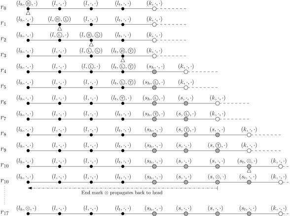
Figure 5: An implantation of DefineSeg on a line $L_{i}$ of four agents depicted as black dots. Each agent uses only its 3 state components $(c_{1},c_{2},c_{3})$, where $c_{1}$ is the label state, $c_{2}$ the transmission state and $c_{3}$ the waiting mark state. In round $r=0$, $L_{i}$ is labelled correctly, starting from a head $l_{h}$ and ends at a tail $l_{t}$ with internal agents $l$. Inactive agents with circles are labelled $k$. First, $l_{h}$ sets $c_{2}\leftarrow\scriptsizeH⃝$. Thereafter, when an active agent $p_{i}$ notices successor $p_{i-1}$ showing “$\scriptsizeH⃝$” , it updates to $c_{2}\leftarrow\scriptsizeH⃝$ (a small triangle indicates this initialisation in rounds $r_{0},r_{1},r_{2},r_{3},$ and $r_{10}$). Agents of label $l$ and $l_{t}$ propagate “$\scriptsizeL⃝$” and “$\scriptsizeT⃝$”, respectively. Whenever an inactive agent sees predecessor presenting a mark, it activates (grey dots) and updates label to corresponding state. Once activating the segment tail $s_{t}$, it propagates an end mark “$\otimes$” back to the head to start CheckSeg.

$S=(p_{1},\ldots,p_{|S|})$ is a Hamiltonian shape

Initial configuration: $S\leftarrow S_{I}$, a line $L\subset S$ of length $k=1,\ldots,\log|S|$, labelled as in Figure 5 topmost

$\scriptsizeH⃝\leftarrow p_{1}.c_{2}$ // head sets a mark in transmission state

repeat

       // each agent acts based on its current label state

       Head $l_{h}$:

       if $(p_{1}.c_{2}=\scriptsizeH⃝)$ then $\cdot\leftarrow p_{i}.c_{2}$ // reset transmission state

      

       if ($p_{i+1}.c_{2}=\otimes$) then $\otimes\leftarrow p_{1}.c_{2}$ // observe end mark; end this sub-phase

      

      

      Active:

       if ($p_{i-1}.c_{2}=\scriptsizeH⃝$) // observe predecessor with head mark

       then

            $\scriptsizeH⃝\leftarrow p_{i}.c_{2}$

             if (inline $p_{i}.c_{1}=l$) then $\scriptsizeL⃝\leftarrow p_{i}.c_{3}$

             if (tail $p_{i}.c_{1}=l_{t}$) then $\scriptsizeT⃝\leftarrow p_{i}.c_{3}$

            

       end if

      if $p_{i-1}.c_{2}=\scriptsizeL⃝$ then $\scriptsizeL⃝\leftarrow p_{i}.c_{2}$ // predecessor shows inline mark

      

       if $p_{i-1}.c_{2}=\scriptsizeT⃝$ then $\scriptsizeT⃝\leftarrow p_{i}.c_{2}$ // predecessor shows tail mark

      

       if $\big{(}(p_{i}.c_{2}=\scriptsizeH⃝\vee\scriptsizeL⃝\vee\scriptsizeT⃝)\wedge p_{i-1}.c_{2}=\cdot\big{)}$ then 

      $p_{i}.c_{2}\leftarrow p_{i}.c_{3}$ // transmit marks

       $\cdot\leftarrow p_{i}.c_{3}$ // rest marks

      

       if $p_{i+1}.c_{2}=\otimes$ then $\otimes\leftarrow p_{i}.c_{2}$ // successor shows end mark

      

       if $p_{i}.c_{2}=\otimes$ then $\cdot\leftarrow p_{i}.c_{2}$ // rest transmission state

      

      

      Inactive:

       if $(p_{i-1}.c_{2}=\scriptsizeH⃝)$ then $s_{h}\leftarrow p_{i}.c_{1}$ // activate to segment head $s_{h}$

      

       if $(p_{i-1}.c_{2}=\scriptsizeL⃝)$ then $s\leftarrow p_{i}.c_{1}$ // activate to insegment $s$

      

       if $(p_{i-1}.c_{2}=\scriptsizeT⃝)$ then 

      $s_{t}\leftarrow p_{i}.c_{1}$ // activate to segment tail $s_{t}$

       $\otimes\leftarrow p_{i}.c_{2}$ // initiate end mark

      

      

until $(p_{1}.c_{2}=\otimes)$

CheckSeg

Algorithm 1 DefineSeg

Lemma 2

DefineSeg requires at most $O(n)$ rounds to define $S_{i}$.

Proof

The head mark “$\scriptsizeH⃝$” shall traverse all agents of the line $L_{i}$ of length $|L_{i}|$ until it arrives at the first inactive agent, taking $O(|L_{i}|)$ rounds. Thus, all other agents on the line propagate marks that take $O(|L_{i}|)$ parallel rounds to reach at their corresponding agents on the next segment. In the worst case, the line can be of length $n/2$, which requires at most $O(n)$ rounds of communication to identity the next segment $S_{i}$ of length $n/2$. ∎

3.2 Check the next segment $S_{i}$

This sub-phase checks the geometrical configuration of the new defined segment $S_{i}$, determining if it is in line with $L_{i}$, perpendicular to $L_{i}$ or contains one turn (L-shape). It aims is to save energy in the system, surpassing one or more of the subsequent sub-phases. First, when $S_{i}$ is in line with $L_{i}$ (see illustrated in Figure 5), both $S_{i}$ and $L_{i}$ already form a single straight line $L_{i+1}$ of double length, and so the next phase $i+1$ begins. This reduces the cost of DrawMap, Push, RecursiveCall and Merge. Second, $S_{i}$ is producing a line perpendicular to $L_{i}$ (see Figure 6(a)), in which case $L_{i}$ just needs to reverse direction and line up with $S_{i}$ to generate $L_{i+1}$, proceeding directly to PushLine and avoiding the extra cost ofDrawMap. Lastly, $S_{i}$ has a single turn (looks like L-shape) (see Figure 6(b)), where it can simply turn at its corner and align with $L_{i}$, create $L_{i+1}$ and save the cost of DrawMap, Push and RecursiveCall. A high-level explanation is provided below.

When $l_{h}$ observes “$\otimes$”, it propagates its own local direction stored in component $c_{4}=a\in A$ by updating $c_{2}\leftarrow c_{4}$. Then, all active agents on the path forward $a$ from $p_{i}$ to $p_{i+1}$ via their transmission components. Whenever a $p_{i}$ with a local direction $c_{4}=a^{\prime}\in A$ notices $a^{\prime}\neq a$, it combines $a$ with its local direction $a^{\prime}$ and changes its transmission component to $c_{2}\leftarrow aa^{\prime}$. After that, if a $p_{i}^{\prime}$ having $c_{4}=a^{\prime\prime}\in A$ observes $a^{\prime\prime}\neq a^{\prime}$, it updates its transmission component into a negative mark, $c_{2}\leftarrow\neg$. All signals are to be reflected by the segment tail $s_{t}$ back to $l_{h}$, which acts accordingly as follows: (1) starts the next sub-phase DrawMap if it observes “$\neg$”, (2) calls Merge to combine the two perpendicular lines if it observes $aa^{\prime}$ or (3) begins a new phase $i+1$ if it receives back its local direction $a$. Algorithm 2 shows the pseud-code of this sub-routine.

$S=(p_{1},\ldots,p_{|S|})$ is a Hamiltonian shape

Initial configuration: $S\leftarrow S_{I}$, a line $L\subset S$ of length $k=1,\ldots,\log|S|$, labelled correctly as in Figure 5 bottommost

$p_{1}.c_{2}\leftarrow p_{1}.c_{4}$ // head emits its direction

repeat

       // each agent acts based on its current label state

       Head $l_{h}$:

       if $(p_{1}.c_{2}=c_{4})$ then $\cdot\leftarrow p_{i}.c_{2}$ // reset transmission state

      

       if ($p_{i+1}.c_{2}=\neg$) then $\neg\leftarrow p_{1}.c_{2}$ // end this sub-phase

      

       if ($p_{i+1}.c_{2}=$ ✓) then start phase $i+1$ // a new phase begins

      

       if ($p_{i+1}.c_{2}=$ └) then PushLine($L$) // $S_{i}$ has one turn

      

      

      Active:

       if ($p_{i-1}.c_{2}=c_{4})$ then $c_{4}\leftarrow p_{i}.c_{2}$ // observe same direction

      

       if $p_{i-1}.c_{2}\neq c_{4}$) then $c_{4}$└ $\leftarrow p_{i}.c_{2}$ // show a turn

      

       if $(p_{i-1}.c_{2}=c_{4}$└) then $\neg\leftarrow p_{i}.c_{2}$ // show another turn

      

       if $(p_{i+1}.c_{2}=\neg$ $\vee$ ✓ $\vee$ └) then $p_{i}.c_{2}\leftarrow p_{i+1}.c_{2}$ // transmit marks backwards

      

       if $(p_{|2L|-1}.c_{2}=c_{4})$ then ✓$\leftarrow p_{|2L|.c2}$// $s_{i}$ transmits mark backwards

      

       if $(p_{|2L|-1}.c_{2}=$ $c_{4}$└) then └$\leftarrow p_{|2L|.c2}$ // $s_{i}$ transmits mark backwards

      

       if $(p_{i-1}.c_{2}\neq\cdot)$ then $\cdot\leftarrow p_{i}.c_{2}$ // reset transmission state

      

      

until $p_{1}.c_{2}=\neg$

DrawMap

Algorithm 2 CheckSeg

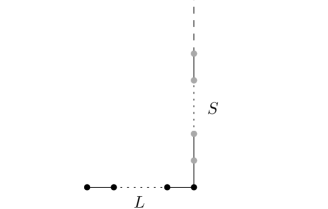
(a) $L_{i}$ is perpendicularly to $S_{i}$.

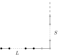
(b) $S_{i}$ has a single turn.

Figure 6: Two configurations of a Hamiltonian path terminates at a straight line $L_{i}$ (in black dots) followed by a segment $S_{i}$ (in grey dots) on the path.

Lemma 3

CheckSeg correctly checks the configuration of $S_{i}$ to be one of the following:

• $S_{i}$ is in line with $L_{i}$.

• $S_{i}$ forms a straight line perpendicular to $L_{i}$.

• $S_{i}$ forms an L-shape.

• $S_{i}$ contains more than one turn.

Proof

This sub-routine starts as soon as the head $l_{h}$ observes the end mark “$\otimes$” of DefineSeg, which means that all agents of the segment $S_{i}$ are active and labelled correctly. Given that, the input configuration of CheckSeg is a Hamiltonian path terminates at straight line $L_{i}$ followed by $S_{i}$, both are composed of $2^{i}$ active agents. All other inactive agents in the rest of the configuration are labelled $k$. During this sub-phase, the active agents use their local directions of the path stored in state $c_{4}$ in which a $p_{i}$ knows each ports incident to predecessor $p_{i-1}$ and successor $p_{i+1}$.

Now, $l_{h}$ updates it transmission state to $c_{2}\leftarrow c_{4}$ where it emits its local direction held in $c_{4}$. Assume without loss of generality, $c_{4}$ holds a local direction pointing to the east neighbour “$\rightarrow$”, then $l_{h}$ performs this state transition: $\delta(l_{h},\otimes,\cdot,\rightarrow)=(l_{h},\rightarrow,\cdot,\rightarrow)$. This arrow “$\rightarrow$” propagates through transmission states to all active agents of $L_{i}$ and $S_{i}$. When a $p_{i-1}$ displays an empty transmission state, each agent $p_{i}$ updates state $c_{2}$ to “$\cdot$”. If “$\rightarrow$” matches a local direction stored on $c_{4}$ of $p_{i}$, then $p_{i}$ transmits the same arrow “$\rightarrow$” from $p_{i-1}$ to $p_{i+1}$. If $p_{i}$ stores a turning arrow (e.g. “$\downarrow$” or “$\uparrow$”) on $c_{4}$, then it updates state $c_{2}$ with a special L-shape mark, “$\rightarrow$└”, which is then passed to $p_{i+1}$. Whenever $p_{j}$ stores a turning arrow and observes $p_{j-1}$ showing “$\rightarrow$└” , $p_{j}$ initiates a negative mark $c_{2}\leftarrow\neg$, which is relayed back to $l_{h}$, calling out for DrawMap. Once $s_{t}$ observes “$\rightarrow$└”, it bounces off the mark “└” back towards $l_{h}$ to start PushLine. Otherwise, $s_{t}$ propagates a special check-mark “✓” backwards, alerting $l_{h}$ that both $L_{i}$ and $S_{i}$ already form a straight line. ∎

Now, we provide analysis of this procedure.

Lemma 4

An execution of CheckSeg requires at most $O(n)$ rounds of communication.

Proof

Consider the worst-case in which the direction mark traverses a $n$-length path and a special mark “✓” bounces off the other end of the path and returns to at the head. This journey takes at most $2n-2$ rounds, during which an agent $p_{i}$, $1\leq i\leq n$, emits the direction mark to $p_{i+1}$ and “✓” to $p_{i-1}$, with the exception of the two endpoints of the path. ∎

3.3 Draw a route map

This local procedure generates a map and computes the shortest possible route with the fewest turns, aiming for the lowest cost and energy consumption. On the square grid, the most efficient way to accomplish this is to draw a rout of a single turn, such as L-shaped routs. For the purpose of connectivity preservation, it can be demonstrated that there exist some worst-case routes in which the line $L_{i}$ may disconnect while travelling towards the tail of $S_{i}$. Essentially, this can be seen in a route where the Manhattan distance between the the line tail $l_{t}$ and the segment tail $s_{t}$ is $\Delta(l_{t},s_{t})\geq|L_{i}|$, for additional information, see [3].

Thus, this distance $\Delta(l_{t},s_{t})$ is important in determining whether to take an L-shaped route directly to $s_{t}$ or to go through an intermediary agent of $S_{i}$ who passes through two L-shaped routes. From our distributed perspective, the Manhattan distance $\Delta(l_{t},s_{t})$ cannot be computed in a straightforward manner due to several challenges, such as individuals with constant local memory and limited computational power. Below, DrawMap addresses these challenges by using $L_{i}$ agents as (1) a distributed binary counter for calculating the distance and (2) a distributed memory for storing local directions of agents, which collectively draw the route map.

This sub-phase computes the Manhattan distance $\Delta(l_{t},s_{t})$ between the line tail $l_{t}$ and the segment tail $s_{t}$, by exploiting ComputeDistance in which the line agents implement a distributed binary counter. First, the head $l_{h}$ broadcasts “$\scriptsizeC⃝$” to all active agents, asking them to commence the calculation of the distance. Once a segment agent $p_{i}$ observes “$\scriptsizeC⃝$”, it emits one increment mark “$\oplus$” if its local direction is cardinal or two sequential increment marks if it is diagonal. The “$\oplus$” mark is forwarded from $p_{i}$ to $p_{i-1}$ back to the head $l_{h}$. Correspondingly, the line agents are arranged to collectively act as a distributed binary counter, which increases by 1 bit per increment mark, starting from the least significant at $l_{t}$.

When a line agent observes the last “$\oplus$” mark, it sends a special mark “$\scriptsize1⃝$” if $\Delta(l_{t},s_{t})\leq|L_{i}|$ or “$\scriptsize2⃝$” if $\Delta(l_{t},s_{t})>|L_{i}|$ back to $l_{h}$. As soon as $l_{h}$ receives “$\scriptsize1⃝$” or “$\scriptsize2⃝$”, it calls CollectArrows to draw a route that can be either heading directly to $s_{t}$ or passing through the middle of $S_{i}$ towards $s_{t}$. In CollectArrows, $l_{h}$ emits “” to announce the collection of local directions (arrows) from $S_{i}$. When “” arrives at a segment agent, it then propagates its local direction stored in $c_{4}$ back towards $l_{h}$. Then, the line agents distribute and rearrange $S_{i}$’s local directions via several primitives, such as cancelling out pairs of opposite directions, priority collection and pipelined transmission. Finally, the remaining arrows cooperatively draw a route map for $L_{i}$ (see Definition 1). The following lemma shows that this procedure calculates $\Delta(l_{t},s_{t})$ in linear time. Below, we give more details of DrawMap.

Definition 1 (A route)

A route is a rectangular path $R$ consisting of a set of cells $R=[c_{1},\ldots,c_{|R|}]$ on $\mathbb{Z}^{2}$, where $c_{i}$ and $c_{i+1}$ are two cells adjacent vertically or horizontally, for all $1\leq i\leq|R|-1$. Let $C$ be a system configuration, $C_{R}$ denotes the configuration of $R$ where $C_{R}\subset C$ defined by $[c_{1},\ldots,c_{|R|}]$.

3.3.1 Distributed Binary Counter.

Due to the limitations of this model, individual agents cannot calculate and keep non-constant numbers in their state. Alternatively, the line $L_{i}$ of $k=2^{i}$ agents can be utilised as a distributed binary counter (similar to a Turing machine tape) which is capable to store up to $2^{k}-1$ unsigned values. This $k$-bit binary counter supports increment which is the only operation we need in this procedure. Each agent’s counter state $c_{5}$ is initially “$\cdot$” and can then hold a bit from $\{0,1\}$. The line tail $l_{t}$ denotes the least significant bit of the counter. An increment operation is performed as follows: Whenever a line agent $p_{i}$ detects $p_{i+1}$ showing an increment mark “$\oplus$”, $p_{i}$ switches counter component $c_{5}$ from “$\cdot$” or 0 to 1 and destroys the “$\oplus$” mark. If $p_{i}$ holds 1 in $c_{5}$, it flips 1 to 0 and redirects the increment mark “$\oplus$” to $p_{i-1}$ (i.e. update the transmission state $c_{2}$ to “$\oplus$”). See an implantation of this counter in Figure 7.

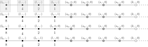
Figure 7: A 4-bit line counter $L_{i}$. Agents of $L_{i}$ and $S_{i}$ are depicted by black grey dots, respectively. The state of an agent is $(c_{1},c_{2},c_{5})$ denoting $c_{1}$ the label, $c_{2}$ transmission and $c_{5}$ counter components, omitting others with no effect. Each shaded area shows a corresponding decimal number. Top: the counter has a decimal value of 0. 2nd: an increment of 1. 3rd: the line tail $l_{t}$ flips state $c_{5}$ from 1 to 0 and updates $c_{2}$ with “$\oplus$”. Bottom: the counter increased by 1 corresponding to a decimal value 2.

3.3.2 ComputeDistance procedure

Initially, the head $l_{h}$ emits a special mark “$\scriptsizeC⃝$” to all active agents, asking them to commence the calculation of the Manhattan distance $\Delta(l_{t},s_{t})$ between the line tail $l_{t}$ and the segment tail $s_{t}$. Whenever a segment agent $p_{i}$ (of label $s_{h},s$ or $s_{t}$) observes $p_{i-1}$ with “$\scriptsizeC⃝$”, it performs one of two transitions: (1) It updates transmission state to $c_{2}\leftarrow\oplus$ if its local direction stored in $c_{4}$ is cardinal (horizontal or vertical) from $\{\rightarrow,\leftarrow,\uparrow,\downarrow\}$, (2) if $c_{4}$ holds a diagonal direction from $\{\nwarrow,\nearrow,\swarrow,\searrow\}$, it receptively updates the transmission and waiting states, $c_{2}$ and $c_{3}$, to “$\oplus$”. Eventually, the segment head $s_{h}$ produces the last special increment mark “$\oplus^{\prime}$”. In principle, any diagonal direction between two cells in a square grid can increase the distance by two (in the Manhattan distance), whereas horizontal and vertical directions always increase it by one.

As a result, all increment marks initiated by segment agents are transmitted backwards to the counter $L_{i}$, in the same way that the propagation of an end mark is described in DefineSeg. Hence, the binary counter increases by 1 bit each time it detects “$\oplus$”, starting from the least significant bit stored in $l_{t}$. Because of transmission parallelism, the binary counter may increase by more than one bit in a single round. When a line agent $p_{i}$ sees predecessor with the last increment mark “$\oplus^{\prime}$”, $p_{i}$ passes “$\scriptsize1⃝$” towards the line head $l_{h}$. This mark “$\scriptsize1⃝$” is altered to “$\scriptsize2⃝$” on its way to $l_{h}$ only if it passes a line agent of a counter state $c_{5}=1$, otherwise it is left unchanged. Eventually, the head $l_{h}$ observes either “$\scriptsize1⃝$”, by which it calls CollectArrows procedure to draw a route map directly to the tail $s_{t}$ of $S_{i}$, or “$\scriptsize2⃝$”, by which it calls CollectArrows to push via a middle agent $s$ towards $s_{t}$. We provide Algorithm 3 of the ComputeDistance procedure below.

$S=(p_{1},\ldots,p_{|S|})$ is a Hamiltonian shape

Initial configuration: a straight line $L_{i}$ and a segment $S_{i}$ labelled as in Figure 7

1. The line head $l_{h}$ propagates counting mark $\scriptsizeC⃝$ along $L_{i}$ and $S_{i}$

2. Once $\scriptsizeC⃝$ arrives at the segment tail $s_{t}$, a segment agent acts as follows:

3. $s_{t}$ sends one increment $\oplus$ back to $l_{h}$ if its direction is cardinal or two $\oplus$ if diagonal

// pipelined transmission

4a. $s$ observes $\oplus$, sends one increment $\oplus$ back to $l_{h}$ if its direction is cardinal or two $\oplus$ if diagonal

4b. $s_{l}$ observes $\oplus$, sends one increment $\oplus^{\prime}$ back to $l_{h}$ if its direction is cardinal or two $\oplus^{\prime}$ if diagonal

5. The distributed counter $L_{i}$ increases by 1 bit each time it receives $\oplus$

6. A line agent observes the last $\oplus^{\prime}$ coming to $L_{i}$, it sends a mark $\scriptsize1⃝$ back to $l_{h}$

7a. Each line agent observes $\scriptsize1⃝$ and has 1 bit, it passes $\scriptsize2⃝$ towards $l_{h}$

7b. Each line agent observes $\scriptsize1⃝$ and has 0 bit, it passes $\scriptsize1⃝$ towards $l_{h}$

7c. Each line agent observes $\scriptsize2⃝$, it passes $\scriptsize2⃝$ towards $l_{h}$

// Manhattan distance $\Delta\leq i$

8a. When $l_{h}$ sees $\scriptsize1⃝$, it calls CollectArrows to draw one L-shaped route

// Manhattan distance $\Delta>i$

8b. Otherwise, $l_{h}$ sees $\scriptsize2⃝$ and calls CollectArrows to draw two L-shaped route

Algorithm 3 ComputeDistance($L_{i},S_{i}$)

Let $\Delta(l_{t},s_{t})$ denote the Manhattan distance between the line tail $l_{t}$ and the segment tail $s_{t}$. The following lemma shows that this procedure calculates $\Delta(l_{t},s_{t})$ in linear time.

Lemma 5

ComputeDistance requires $O(|L_{i}|)$ rounds to compute $\Delta(l_{t},s_{t})$.

Proof

Consider an input configuration labelled $(\overbrace{l_{h},\ldots,l,\ldots,l_{t}}^{L_{i}},\overbrace{s_{h},\ldots,s,\ldots,s_{t}}^{S_{i}},$ $k,\ldots,k)$, starting at a line head $p_{1}$ of label $l_{h}$, where $|L_{i}|=|S_{i}|$. We only show affected states in this proof. Initially, $l_{h}$ emits a counting mark “$\scriptsizeC⃝$” by updating transmission state to $p_{1}.c_{2}\leftarrow\scriptsizeC⃝$, then $l_{h}$ resets transmission state to $c_{2}\leftarrow\cdot$ in subsequent rounds. Once an active agent $p_{i}$ in round $r_{j-1}$ (where $j\leq 2|L_{i}|$) detects predecessor showing state $p_{i-1}.c_{2}=\scriptsizeC⃝$, it updates transmission state to $p_{i}.c_{2}\leftarrow\scriptsizeC⃝$ in $r_{j}$ and then resets $p_{i}.c_{2}\leftarrow\cdot$ in $r_{j+1}$. Upon arrival of “$\scriptsizeC⃝$” at $s_{t}$, its predecessor changes transmission state to $c_{2}\leftarrow\oplus$ and puts another increment mark in waiting state $c_{3}\leftarrow\oplus$ if it stores a diagonal arrow in its local direction $c_{4}$.

Due to the goal of counting, the direction of $s_{t}$ is dropped. Each segment agent $p_{i}$ of label $s_{h}$ and $s$ observes a successor presenting state $p_{i+1}.c_{2}=\oplus$ in round $r_{j-1}$, then the following transitions apply in $r_{j}$: (1) $p_{i}.c_{2}\leftarrow\oplus$ if $p_{i+1}.c_{2}\leftarrow\oplus$, (2) if $p_{i}.c_{2}\leftarrow\oplus$ if $p_{i+1}.c_{2}\leftarrow\cdot$ and $p_{i}.c_{3}\leftarrow\oplus$, (3) the head of segment $s_{h}$ sets $p_{i}.c_{2}\leftarrow\oplus^{\prime}$ if $p_{i+1}.c_{2}\leftarrow\cdot$ and $p_{i}.c_{3}\leftarrow\oplus$ and (4) $p_{i}.c_{2}\leftarrow\cdot$ if $p_{i+1}.c_{2}\leftarrow\cdot$ and $p_{i}.c_{3}\leftarrow\cdot$.

Correspondingly, the line agents (of labels $l_{h}$, $l$ and $l_{t}$) behave as a binary counter described above and illustrated in Figure 7. When a line agent $p_{i}$ detects “$\oplus$” in the state of $p_{i+1}$ in round $r_{j-1}$, it updates state based on one of theses transitions in round $r_{j-1}$: (1) $p_{i}.c_{5}\leftarrow 1$ if $p_{i}.c_{5}\leftarrow\cdot$ or $p_{i}.c_{5}\leftarrow 0$ or (2) $p_{i}.c_{5}\leftarrow 0$ and $p_{i}.c_{2}\leftarrow\oplus$ if $p_{i}.c_{5}\leftarrow 1$. In the case where the last increment mark “$\oplus^{\prime}$” detected by $p_{i}$ in round $r_{j-1}$, then $p_{i}$ updates state to $p_{i}.c_{2}\leftarrow\scriptsize1⃝$ in $r_{j}$. When $p_{i-1}$ observes $\scriptsize1⃝$, then it updates states to either (1) $p_{i-1}.c_{2}\leftarrow\scriptsize1⃝$ if $p_{i-1}.c_{5}=0$ or (2) $p_{i-1}.c_{2}\leftarrow\scriptsize2⃝$ if $p_{i-1}.c_{5}=1$. Thus, the mark “$\scriptsize2⃝$” is sent back to the head $l_{h}$, which finally sees either ‘$\scriptsize1⃝$” or “$\scriptsize2⃝$” and acts appropriately (calls CollectArrows procedure). The counter size is sufficient to calculate $\Delta(l_{t},s_{t})$ because the since the worst-case would distance is $|L_{i}|-2$.

Now, we analyse the cost of communication of this procedure in a number of rounds. First, the counter mark “$\scriptsizeC⃝$” goes on a journey that takes $t_{1}=2|L_{i}|=O(|L_{i}|)$ rounds. That is, the pipelined transmission of increment marks requires at most $t_{2}=O(|L_{i}|)$ parallel rounds of communication. Moreover, the marks “$\scriptsize1⃝$” or “$\scriptsize2⃝$” travel to the head $l_{h}$ within at most $t_{3}=O(|L_{i}|)$. Altogether, the total running time is bounded by $t=t_{1}+t_{2}+t_{3}=O(|L_{i}|)$ parallel rounds. ∎

3.3.3 CollectArrows procedure

Informally, the distance obtained from the ComputeDistance procedure can be (1) equal or less than the line length $|L_{i}|$ ($l_{h}$ observes this mark “$\scriptsize1⃝$”) or (2) greater than $|L_{i}|$ ($l_{h}$ observes “$\scriptsize2⃝$”). In case (1), it propagates a special collection mark “” through all active agents until it reaches the segment tail $s_{t}$. When “” arrives, $s_{t}$ broadcasts its local arrow in $c_{4}$ back to $l_{h}$ via active agent transmission states. This journey accomplishes the following: (a) Gathers arrows similar to $s_{t}$ and puts them in priority transmission. (b) Eliminates pairs of opposite arrows and replaces them with a hash mark “#”. (c) Arranges the arrows on $L_{i}$’s distributed memory. In case (2), $l_{h}$ emits a special mark “$\scriptsizeM⃝$” to $s_{h}$, defining a midpoint on $S_{i}$ through which the line $L_{i}$ passes towards $s_{t}$.

Now, $s_{h}$ propagates two marks down $s_{t}$, a fast mark “$\tinym1⃝$” is transmitted every round and a slow mark moves three rounds slower “$\tinym2⃝$”. The fast mark “$\tinym1⃝$” bounces off $s_{t}$, where both “$\tinym1⃝$” and “$\tinym2⃝$” meet in a $S_{i}$ middle agent $p_{j}$, which changes label to $s_{t}^{\prime}$ and a successor $p_{j+1}$ switches to $s_{h}^{\prime}$. This temporally divides $S_{i}$ into two segments, $S_{i}^{1}=s_{h},\ldots,s_{t}^{\prime}$ and $S_{i}^{2}=s_{h}^{\prime},\ldots,s_{t}$. The middle agent $s_{t}^{\prime}$ propagates “$\scriptsizeM⃝$” to tell $l_{h}$ that a midpoint has been identified. Case (1) is then repeated twice to collect arrows from $S_{i}^{1}$ and $S_{i}^{2}$ and distribute them into the line agents (distributed memory). After that, Push($S$) begins. Algorithm 4 presents the pseudocode that briefly formulates this procedure.

Input: a straight line $L_{i}$ and a segment $S_{i}$

// priority and pipelined transmission, see text for details

(A) Line head $l_{h}$ observes $\scriptsize1⃝$

1. $l_{h}$ propagates collection mark

2. Each active agent $p_{i}$ emits   to $p_{i+1}$

3. $s_{t}$ observes $\scriptsize1⃝$ and propagates its direction $d$ in $c_{4}$, $c_{2}\leftarrow c_{4}$

4. Each segment agent $p_{i}$ passes a direction to $p_{i-1}$

5. Distribute directions into the line agents

6. Rearrangement of directions

7. Push($S$) begins

(B) Line head $l_{h}$ observes $\scriptsize2⃝$

1. $l_{h}$ propagates a midpoint mark $\scriptsizeM⃝$

2. Each line agent $p_{i}$ broadcasts $\scriptsizeM⃝$ to $p_{i+1}$

3. $s_{h}$ sees $\scriptsizeM⃝$, then emits fast $\tinym1⃝$ and slow $\tinym2⃝$ waves down to $s_{t}$

4. $\tinym1⃝$ bounces off $s_{t}$ and meets $\tinym2⃝$ at middle agent $p_{j}$ with label changed to $s_{t}^{\prime}$

5. $s_{t}^{\prime}$ propagates $\scriptsizeM⃝$ to $l_{h}$

6. Once $l_{h}$ sees $\scriptsizeM⃝$ again, it goes to (A)

Algorithm 4 CollectArrows($L_{i},S_{i}$)

The following lemma proves the correctness and analysis of CollectArrows.

Figure 8: Drawing a map: from top-left a path across occupied cells and corresponding local arrows stored on state $c_{4}$ in top-tight, where the diagonal directions, “$\searrow$” and “$\nearrow$”, are interpreted locally as, “$\downarrow\rightarrow$” and “$\uparrow\rightarrow$”. The bottom shows a route map drawn locally on state $c_{6}$ of each line agent.

Lemma 6

The CollectArrows procedure completes within $O(|L_{i}|)$ rounds.

Proof

Given an initial configuration defined in Lemma 5. Assume the Manhattan distance $\delta(l_{t},s_{t})\leq|L_{i}|$. For simplicity, we prove (A) in algorithm 4 showing only affected states. Once $l_{h}$ observes $\scriptsize1⃝$, it emits a collection mark “”, which then transfers forwardly among active agents until it reaches $s_{t}$, similar to counting mark transmission described previously in Lemma 5. When $s_{t}$ detects “”, it updates transmission state $c_{2}$ with its local direction held in $c_{4}=d$; recall that $d$ is an arrow that locally shows where the Hamiltonian path comes in and out, $d\in\{\rightarrow,\leftarrow,\downarrow,\uparrow,\nwarrow,\nearrow,\swarrow,\searrow\}$.

In what follows, we distinguish between cardinal $\{\rightarrow,\leftarrow,\downarrow,\uparrow\}$ and diagonal directions $\{\nwarrow,\nearrow,\swarrow,\searrow\}$. Figure 8 shows how local arrows are assigned to agents according to the Hamiltonian path. For a cardinal local direction, $s_{t}$ updates transmission state to $c_{2}\leftarrow d$ and marks local direction state with a star $c_{4}\leftarrow d^{\star}$, indicating that $d$ has been collected. A diagonal local direction between any two neighbouring cells on the two-dimensional square grid is made up of two cardinal arrows, such as $\nwarrow$ is composed of $\uparrow$ and $\leftarrow$. In other words, an agent needs to move two steps to occupy an adjacent diagonal cell. For example, if $s_{t}$ stores a diagonal direction in $c_{4}$, it puts $d^{1}$ on transmission $c_{2}\leftarrow d^{1}$, $d^{2}$ on waiting state $c_{3}\leftarrow d^{2}$, and marks it with a star, $c_{4}\leftarrow d^{\star}$. Next round, the transmission state of $s_{t}$ resets $c_{2}\leftarrow\cdot$ if $c_{3}$ is empty or sets $c_{2}\leftarrow c_{3}$ if $c_{3}$ contains an arrow.

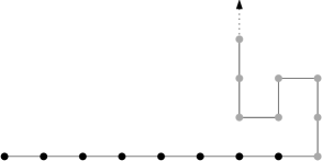
Figure 9: A configuration of $L_{i}$ (black dots) and $S_{i}$ (grey dots).

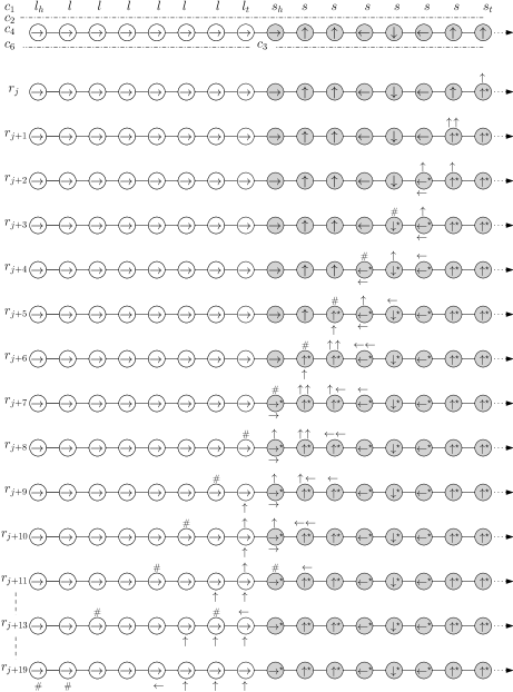
Figure 10: An implementation of the arrows collection on the shape in Figure 9. For better visibility, we represent $L_{i}$ and $S_{i}$ as a tab, where white nodes depict $L_{i}$ and greys indicate $S_{i}$. Topmost shape shows that each agent represents its local direction $c_{4}$ inside nodes, label $c_{1}$ and transmission $c_{2}$ above nodes, waiting $c_{3}$ (only for segment agents) and map state $c_{6}$ (only for line agents) below nodes. The process starts from round $r_{j}$ downwards. See Lemma 6 for a full description.

We now show the priority and pipelined collection of local arrows of $S_{i}$ (in Algorithm 4). Assume a direction (arrow) $d^{+}$ transmits from the segment tail $s_{t}$, travelling through transmission states via an active agent $p_{i+1}$ to $p_{i}$. When $d^{+}$ encounters an opposite arrow $d^{-}$ recorded in transmission state $p_{i}.c_{2}$, both are erased and replaced by the hash sign “#”. If $d^{+}$ and $d^{+}$ are similar, both take priority in $c_{2}$. If $d^{+}$ observes a perpendicular arrow $\perp d$, $d^{+}$ is placed in $c_{2}$ and $\perp d$ in waiting state $c_{3}$. For example, Figure 9 depicts a configuration of $S_{i}$ consisting of 8 agents, the arrows of which are collected in Figure 10. Full details for the associated transitions per active agent are provided below.

Given a segment agent $p_{i}$ of label $s$ and $s_{t}$ in round $r_{j-1}$, where $j\leq 2|L_{i}|$. Then we show how $p_{i}$ acts when the direction is either cardinal or diagonal. Consider $p_{i}$ of an uncollected cardinal direction $d_{i}$ observes $p_{i+1}$ showing a direction $d_{i+1}$, two directions $d_{i+1}(d_{i+1}^{1}d_{i+1}^{2})$ or # in transmission component $c_{2}$. Then, $p_{i}$ updates its state in $r_{j}$ as follows: (1) Set $d_{i+1}$ or $d_{i+1}^{1}$ in transmission $p_{i}.c_{2}\leftarrow p_{i+1}.c_{2}$, put $d_{i}$ in waiting $p_{i}.c_{3}\leftarrow p_{i}.c_{4}$ and mark it $p_{i}.c_{4}\leftarrow d_{i}^{\star}$ if $d_{i}$ is perpendicular to $d_{i+1}$, such as $\rightarrow$ and $\uparrow$. (2) Set $p_{i}.c_{2}\leftarrow$ #, put $d_{i}$ in waiting $p_{i}.c_{3}\leftarrow p_{i}.c_{4}$ and mark its local direction $p_{i}.c_{4}\leftarrow d_{i}^{\star}$ if $d_{i}$ and $d_{i+1}$ are a pair of opposite arrows, such as $\uparrow$ and $\downarrow$. (3) Set both directions $d_{i+1}$ and $d_{i}$ in transmission $p_{i}.c_{2}\leftarrow d_{i+1}d_{i}$, resets $c_{3}\leftarrow\cdot$ and mark $d_{i}$ with a star $p_{i}.c_{4}\leftarrow d_{i}^{\star}$ if $d_{i}$ and $d_{i+1}$ are a pair of same arrows, such as $\uparrow$ and $\uparrow$. When a cardinal direction is already collected $d_{i}^{\star}$, $p_{i}$ sets $d_{i+1}$ or $d_{i+1}^{1}$ in transmission $p_{i}.c_{2}\leftarrow p_{i+1}.c_{2}$. If $d_{i+1}$ ( or $d_{i+1}^{1}$) and $c_{3}=d_{i}$ are similar, then $p_{i}$ sets $p_{i}.c_{2}\leftarrow d_{i+1}d_{i}$ (or $p_{i}.c_{2}\leftarrow d_{i+1}^{1}d_{i}$) and resets $p_{i}.c_{3}\leftarrow\cdot$. If $p_{i+1}.c_{2}$ is empty, then $p_{i}$ puts waiting direction in transmission $p_{i}.c_{2}\leftarrow p_{i}.c_{4}$ or rests $p_{i}.c_{2}\leftarrow\cdot$, otherwise.

In the second case, $p_{i}$ holds an uncollected diagonal arrow $d_{i}(d_{i}^{1}d_{i}^{2})$ in $r_{j-1}$, so it performs one of the following in $r_{j}$: (1) Set $d_{i+1}$ and $d_{i}^{1}$ in transmission $p_{i}.c_{2}\leftarrow d_{i+1}d_{i}^{1}$, put $d_{i}^{2}$ in waiting $p_{i}.c_{3}\leftarrow d_{i}^{2}$ and mark $d_{i}$ with a star $p_{i}.c_{4}\leftarrow d_{i}^{\star}$ if $d_{i+1}$ and $d_{i}^{1}$ (or $d_{i}^{2})$ are similar, such as $\uparrow$ and $\nwarrow=(\uparrow\leftarrow)$. (2) Set $p_{i}.c_{2}\leftarrow$ #, put $d_{i}^{2}$ in waiting $p_{i}.c_{3}\leftarrow d_{i}^{2}$ and mark the direction $d_{i}^{\star}$ if $d_{i+1}$ is opposites to either $d_{i}^{1}$ or $d_{i}^{2}$, such as $\uparrow$ and $\swarrow=(\downarrow\leftarrow)$. If a diagonal arrow has been already collected $d_{i}^{\star}$, then $p_{i}$ sets $d_{i+1}$ or $d_{i+1}^{1}$ in transmission $p_{i}.c_{2}\leftarrow p_{i+1}.c_{2}$. If $d_{i+1}$ (or $d_{i+1}^{1}$) and waiting direction $c_{3}=d_{i}$ are the same, then $p_{i}$ updates to $p_{i}.c_{2}\leftarrow d_{i+1}d_{i}$ (or $p_{i}.c_{2}\leftarrow d_{i+1}^{1}d_{i}$) and resets $p_{i}.c_{3}\leftarrow\cdot$. If $p_{i+1}.c_{2}$ is empty then, $p_{i}$ puts waiting direction in transmission $p_{i}.c_{2}\leftarrow p_{i}.c_{4}$ or rests $p_{i}.c_{2}\leftarrow\cdot$, otherwise.

Meanwhile, the line agents receive the collected arrows and divide them among respective states as follows. Let $p_{i}$ denote a line agent, holding a map state $p_{i}.c_{6}=\cdot$, observes $p_{i+1}$ showing a direction $d_{i+1}$ or a hash sign “#”. Then, $p_{i}$ acts accordingly: (1) $p_{i}.c_{6}\leftarrow d_{i+1}$, (2) if $p_{i}$ is $l_{h}$ or sees $p_{i-1}$ with a map state $c_{6}=$#, then $p_{i}.c_{6}\leftarrow$#. Whenever $p_{i}.c_{6}\neq\cdot$ detects $p_{i+1}.c_{2}=d$ or $p_{i+1}.c_{2}=$# , then $p_{i}$ updates state to $d_{i+1}$ or “#” if $p_{i-1}.c_{6}=\cdot$. Once the line tail $l_{t}$ of a non-empty map component detects $p_{i+1}.c_{2}=\cdot$, it propagates a special mark “✓” via line agents towards $l_{h}$, announcing the completion of arrows collection.

Now, let us discuss (B) in algorithm 4 in which $l_{h}$ observes “$\scriptsize2⃝$”, indicating the Manhattan distance $\delta(l_{t},s_{t})>|L_{i}|$. In reaction to this, $l_{h}$ emits the midpoint mark “$\scriptsizeM⃝$” forwardly down the line agents towards $s_{h}$. Once $s_{h}$ detects “$\scriptsizeM⃝$”, it emits two waves via the segment, fast “$\tinym1⃝$” and slow “$\tinym2⃝$”. The fast wave “$\tinym1⃝$” moves from $p_{i}$ to $p_{i+1}$ every round, while the slow wave “$\tinym2⃝$” passes every three rounds. In this way, the fast wave “$\tinym1⃝$” bounces off $s_{t}$ and meets ‘$\tinym2⃝$” at a middle agent $p_{i}^{\prime}$ of $S_{i}$ which updates label to $s_{t}^{\prime}$, and $p_{i+1^{\prime}}$ changes label to $s_{h}^{\prime}$ as well. See a demonstration in Figure 11. Consequently, $S_{i}$ is temporarily divided into two halves $S_{i}^{1}$ and $S_{i}^{2}$ labelled:

$$(\ldots,\overbrace{s_{h},\ldots,s,\ldots,s_{t}^{\prime}}^{S_{i}^{1}},\overbrace{s_{h}^{\prime},\ldots,s,\ldots,s_{t}}^{S_{i}^{2}},\ldots).$$

Now, $s_{t}^{\prime}$ emits the “$\scriptsizeM⃝$” mark back to $l_{h}$ via transmission states, from $p_{i}$ to $p_{i-1}$. Upon arrival of “$\scriptsizeM⃝$”, $l_{h}$ invokes the sub-procedure (A) to begin collection on the first half $S_{i}^{1}$ and Push($S$) to move towards $s_{t}^{\prime}$, after which $l_{h}$ calls (A) again to travel into $s_{t}$.

We argue that the line $L_{i}$ always has sufficient memory to store all collected arrows. The Manhattan distance will always be $\delta(l_{t},s_{t})>|L_{i}|$ if the segment $S_{i}$ has at least one diagonal connection. Consider the worst-case scenario of a diagonal segment in which each agent $p_{i}$ gains a local diagonal direction at a cost of two cardinal arrows. Recall that each agent can store two arrows in its state, in $c_{6}$ and $c_{7}$. Given that, in the worst-case the segment contains a total of $2|S_{i}|$ local arrows. Thus, by applying (A) twice in each half of $S_{i}$, each single arrow of $S_{i}$ will find a room in $L_{i}$.

We now calculate the running time of the CollectArrows($L_{i},S_{i}$) procedure on a number of rounds. Starting from steps 1 and 2 of (A), the “” mark takes a journey from $l_{h}$ to $s_{t}$ requiring at most $t_{1}=|L_{i}|+|S_{i}|=O(|L_{i}|)$ rounds. Then, the pipelined collection and rearrangement of arrows in steps 3-6, require at most a number of parallel rounds equal asymptotically to the length of $|S_{i}|+|L_{i}|$, namely $t_{2}=O(|L_{i}|)$. Moreover, the cost of “✓” transmission takes time $t_{3}=|L_{i}|$ rounds. In (B), the propagation of “$\scriptsizeM⃝$” costs $t_{4}=|L_{i}|$, another cost $t_{5}=3|S_{i}|$ is preserved for (1) and (2), which is the communication of fast “$\tinym1⃝$” and slow “$\tinym2⃝$” and the return of “$\scriptsizeM⃝$” to the head, respectively. Hence, (A) costs at most $t_{A}=t_{1}+t_{2}+t_{3}=O(|L_{i}|)$ parallel rounds of communication, whereas (B) requires at most $t_{B}=t_{4}+t_{5}=O(|L_{i}|)$. The same bound holds in the worst-case by applying (A) twice. Therefore, this procedure requires a total number of at most $T=2t_{A}+t_{B}=O(|L_{i}|)$ parallel rounds to draw a rout map. ∎

Figure 11: A fast “$\tinym1⃝$” and slow “$\tinym2⃝$” wave meeting at the middle of $S_{i}$ of 8 agents. Observe that “$\tinym1⃝$” moves every round, while “$\tinym2⃝$” is three rounds slower.

Finally, ComputeDistance and CollectArrows procedures completes the DrawMap sub-phase. By Lemmas 5 and 6, we conclude that:

Lemma 7

DrawMap draws a map within $O(|L_{i}|)$ rounds.

3.4 Push the next segment $S_{i}$

Unlike all previous sub-phases, the transformation now allows individuals to perform line movements on the grid, taking advantage of their linear-strength pushing mechanism. That is, a straight line $L_{i}$ of $2^{i}$ agents occupying a column or row of $2^{i}$ consecutive cells on the square grid can be pushed in a single step depending on its orientation in parallel vertically or horizontally in a single-time step. Furthermore, $L_{i}$ has the ability to change direction or turn from vertical to horizontal and vice versa.

A variety of obstacles must be overcome in order to translate the global coordinator of line moves into a system of homogeneous agents capable of only local vision and communication. One of the most essential challenges is timing: an individual agent moving the line must know when to start and stop pushing. Otherwise, it may disconnect the shape and break the connectivity-preservation requirement. Further, the line may change direction and turn around while pushing; hence, it must have some kind of local synchronisation over its agents to ensure that everyone follows the same route and no one is pushed off. Failure to do so may result in a loss of connectivity, communication, or the displacement of other agents in the configuration. Moreover, pushing a line does not necessarily traverse through free space of a Hamiltonian shape; consequently, a line may walk along the remaining configuration of agents while ensuring global connectivity at the same time. However, we were able to address all of these concerns in Push, which will be detailed below.

After some communication, $l_{h}$ observes that $L_{i}$ is ready to move and can start Push now. It synchronises with $l_{t}$ to guide line agents during pushing. To achieve this, it propagates fast “$\tinyp1⃝$” and slow “$\tinyp2⃝$” marks along the line, “$\tinyp1⃝$” is transmitted every round and “$\tinyp2⃝$” is three rounds slower (shown early in DrawMap). The “$\tinyp1⃝$” mark reflects at $l_{t}$ and meets “$\tinyp2⃝$” at a middle agent $p_{i}$, which in turn propagates two pushing signals “$\tinyP⃝$” in either directions, one towards $l_{h}$ and the other heading to $l_{t}$. This synchronisation liaises $l_{h}$ with $l_{t}$ throughout the pushing process, which starts immediately after “$\tinyP⃝$” reaches both ends of the line at the same time. Recall the route map has been drawn starting from $l_{t}$, and hence, $l_{t}$ moves simultaneously with $l_{h}$ according to a local map direction $\hat{a}\in A$ stored in its map component $c_{6}$.

Through this synchronisation, $l_{t}$ checks the next cell $(x,y)$ that $L_{i}$ pushes towards and tells $l_{h}$, whether it is empty or occupied by an agent $p\not\in L_{i}$ in the rest of the configuration. If $(x,y)$ is empty, then $l_{h}$ pushes $L_{i}$ one step towards $(x,y)$, and all line agents shift their map arrows in $c_{6}$ forwardly towards $l_{t}$. If $(x,y)$ is occupied by $p\not\in L_{i}$, then $l_{t}$ swaps states with $p$ and tells $l_{h}$ to push one step. Similarly, in each round of pushing a line agent $p_{i}$ swaps states with $p$ until the line completely traverses the drawn route map and restores it to its original state. Figure 16 shows an example of pushing $L_{i}$ through a route of empty and occupied cells. In this way, the line agents can transparently push through a route of any configuration and leave it unchanged. Once $L_{i}$ has traversed completely through the route and lined up with $s_{t}$, then RecursiveCall begins. Algorithm 5 provides a general procedure of Push.

Input: a straight line $L_{i}$ and a segment $S_{i}$

The line head $l_{h}$ observes the completion of DrawMap

repeat

       $l_{h}$ emits a mark to $l_{t}$ to start pushing // $l_{t}$ sees empty or non-empty cell

       if $c_{6}=d_{l_{t}}$ point to empty cell // local arrow of $l_{t}$ points to empty cell

       then

            $l_{h}$ syncs $L_{i}$: update states and push one step

       end if

      

      if $c_{6}=d_{l_{t}}$ point to non-empty cell $k$ then

             $l_{t}$ activates $k$

            $l_{h}$ syncs $L_{i}$ // swap and update states as described in text

            

            $L_{i}$ pushes one step

       end if

      

until $l_{h}$ swaps labels with $s_{h}$

RecursiveCall begins

Algorithm 5 Push

Figure 12: Synchronising 8 agents that were started in Figure 11 where the halving procedure repeats until all agents reach a synchronised state.

3.4.1 Agents synchronisation

Many agent behaviours, including state swapping and line movements (parallel pushing), are realised to be very efficient in the centralised systems of a global coordinator. In contrast, the constraints in this model make these simple tasks difficult, as individuals with limited knowledge cannot keep track of others during the transformation. This may result in the disconnection of the whole shape, a modification in the rest of the configuration or even the loss of a chain of actions that halts the transformation process. However, the synchronisation of agents can assist to tackle such an issue where individuals can organise themselves to eventually arrive at a state in which all of them conduct tasks concurrently. This concept is similar to a well-known problem in cellular automata known as the firing squad synchronisation problem, which was proposed by Myhill in 1957. McCarthy and Minsky provided a first solution to this problem [30]. The following lemma demonstrates how their solution can be translated to our model in order to coincide a Hamiltonian path of $n$ agents in such a way that they can perform concurrent actions in linear time.

Lemma 8 (Agents synchronisation)

Let $P$ denote a a Hamiltonian path of $n$ agents on the square grid, starting from a head $p_{1}$ and ending at a tail $p_{n}$, where $p_{1}\neq p_{n}$. Then, all agents of $P$ can be synchronised in at most $O(n)$ rounds.

Proof

From [30], the strategy consists of two cases, even and odd number of agents. First, the head $p_{1}$ emits fast mark “$\tinym1⃝$” and slow mark “$\tinym2⃝$” towards the tail $p_{n}$. The “$\tinym1⃝$” mark is communicated from $p_{i}$ to $p_{i+1}$ via transmission components in each round, while is transmitted from $p_{i}$ to $p_{i+1}$ every three rounds. When “$\tinym1⃝$” reaches the other end of the path $p_{n}$, it returns to $p_{1}$. Thus, the two marks collide exactly in the middle (see an example in Figure 11). Now, the two agents who witness the collision update to a special state, which will effectively split $P$ into two sub-paths. Both agents repeat the same procedure in each half of length $n/2$ in either direction of $P$. Repeat this halving until all agents reach a special state (collision witness) in which they all perform an action simultaneously. An implementation of this synchronisation is depicted in Figure 12.

Assume a path $P$ of $n$ odd agents in which $p_{1}$ emits, “$\tinyp1⃝$” and “$\tinyp2⃝$” along $P$. In this case, the two marks meet in a slightly different way, at an exact single middle agent $p_{i}$ on $P$. This agent $p_{i}$ observes a predecessor $p_{i-1}$ showing “$\tinym2⃝$” and successor $p_{i+1}$ showing “$\tinym1⃝$” in transmission state and responds by switching into another special state that allows it to play two roles. That is, it emits “$\tinyp1⃝$” and “$\tinyp2⃝$” to both directions of $P$, this effectively splits $P$ into two sub-paths of length $n/2-1$ each. Now, repeat the process in each half until the two marks intersect in the middle, at which point two agents notice the collision and change to a special state. In the same way, divide until all agents have updated to a synchronised state. Figure 13 depicts the synchronisation in the odd case.

Now, we are ready to describe the state transitions. In the first round $r_{j}$, $p_{1}$ updates to $p_{1}.c_{2}\leftarrow\tinym1⃝$ and combines “$\tinym2⃝$” with “$w$” in waiting state, $p_{1}.c_{3}\leftarrow\tinym2⃝w$. Next round $r_{j+1}$, $p_{1}$ updates state to $p_{1}.c_{3}\leftarrow\tinym2⃝$ and $p_{1}.c_{2}\leftarrow\cdot$. In the third round $r_{j+2}$, $p_{1}$ updates transmission state to $p_{1}.c_{2}\leftarrow\tinym2⃝$. Whenever $p_{i}$ notices: (1) $p_{i-1}$ (or $p_{i+1}$) showing “$\tinym1⃝$”, $p_{i}$ shifts transmission to $p_{i}.c_{2}\leftarrow\tinym1⃝$ and $p_{i-1}$ o(r $p_{i+1}$) rests their transmission next round. (2) $p_{i-1}$ (or $p_{i+1}$) showing “$\tinym2⃝$”, $p_{i}$ updates waiting state to $p_{i}.c_{3}\leftarrow\tinym2⃝w$ and $p_{i-1}$ (or $p_{i+1}$) rests their transmission next round. (3) $p_{i+1}$ showing “$\tinym1⃝$” and $p_{i-1}$ presenting “$\tinym2⃝$” (or vice versa), $p_{i}$ updates to another special state and repeats (1). When both $p_{i}$ and $p_{i+1}$ are presenting “$\tinym1⃝$” and “$\tinym2⃝$”, they update into a special state and repeat the procedure of $p_{1}$ in either directions. Repeat until all agents and their neighbours reach a special state where all are synchronised.

Let us now analyse the runtime of this synchronisation in a number of rounds. The fast mark “$\tinym1⃝$” moves along $P$ taking $n$ rounds plus $n/2$ to walks back to the centre in a total of at most $3n/2$ rounds. The same bound applies to the slow mark “$\tinym2⃝$” arriving and meeting “$\tinym1⃝$” in the middle. The whole procedure is now repeated on the two halves of length $n/2$, each takes $3n/4$ rounds. This adds up to a total $\sum_{i=1}^{n}3n/2^{i}=3n/2+3n/4+\ldots+0=3n(1/2+1/4+\ldots+0)=3n(1)=3n$. Therefore, this synchronisation requires at most $O(n)$ rounds of communication. ∎

Figure 13: An example of synchronising 7 agents - odd case.

Now, we show that under this model a number of consecutive agents forming a straight line $L_{i}$, can traverse transparently through a route $R$ of cells on the grid of any configuration $C_{R}$ exploiting only their local knowledge, without breaking the connectivity of the whole shape.

Lemma 9

Let $L_{i}$ denote a terminal straight line and $R$ be a rectangular path of any configuration $C_{R}$, starting from a cell adjacent to the tail of $L_{i}$, where $R\leq 2|L_{i}|-1$. Then, there exists a distributed way to push $L_{i}$ along $R$ without breaking connectivity.

Proof

In Algorithm 5, the line head $l_{h}$ observes the collection mark “✓” indicating the completion of DrawMap($S$), which draws a route $R$ (see Definition 1). As a result, $l_{h}$ emits the question mark “$?$” to $l_{t}$, which will broadcast via line agent transmission states from $p_{i}$ to $p_{i+1}$. Once ‘$?$” arrives there, $l_{t}$ checks whether its map arrow $d_{l_{t}}$ points to an empty or occupied cell, and if so, it emits a special mark “$\tinyY⃝$” back to $l_{h}$ indicating that a rout is free to push. By an application of Lemma 8, $l_{h}$ synchronises all line agents to reach a concurrent state in which the following actions occur concurrently: (1) $l_{h}$ pushes $L_{i}$ one position towards $l_{t}$, based on its local direction on push state $c_{7}$. (2) $l_{t}$ pushes one position based on its map arrow $c_{6}$ either in line direction or perpendicular to $L_{i}$. In the latter, $l_{t}$ updates state to $c_{4}\leftarrow c_{6}$ and tells predecessor to turn next round. In general, (3) If $p_{i}$ turns, it updates local direction $c_{4}\leftarrow c_{6}$, and $p_{i-1}$ updates push component $p_{i-1}.c_{7}\leftarrow p_{i}.c_{6}$. (4) $p_{i}$ of a present push component $c_{7}$ moves one step in the direction held in $c_{7}$, which then rests to $p_{i}.c_{7}\leftarrow\cdot$. (5) All line agents shift local map direction forwardly towards $l_{t}$, $p_{i}.c_{6}\leftarrow p_{i-1}.c_{6}$. Repeat these transitions until $l_{t}$ encounters the segment tail $s_{t}$ on the route through which $l_{t}$ tells $l_{h}$ to sync and push again, while $l_{t}$ and $s_{t}$ swaps their states. Hence, any $p_{i}$ meets $s_{t}$, they swap states and rest their $c_{6}$. Eventually, $l_{h}$ stops pushing once it meets and swaps states with $s_{t}$. An example is shown in Figure 14.

Figure 14: A line $L_{i}$ of four agents pushing through a route of empty cells towards $s_{t}$. All affected states ($c_{4},c_{5}$ and $c_{7}$) are shown inside each occupied cell.

During pushing through an L-shape route $R$, $L_{i}$ may turn one or at most three times. In the following, we show that the number of turns depends on the orientation of both $L_{i}$ and $R$. Without loss of generality, assume a horizontal $L_{i}$ turning at a corner towards $s_{t}$, such as Figure 14 where $L_{i}$ will temporally divide into two perpendicular sub-lines while traversing to $s_{t}$. By a careful application of Lemma 8, both can be synchronised and organised to perform two parallel pushing where $l_{h}$ liaises with $l_{t}$ and push the two perpendicular sub-lines concurrently. Now, assume $s_{t}$ is placed two cells above the middle of $L_{i}$, resulting in a route $R$ of three turns along which $L_{i}$ temporally transforms into three perpendicular sub-lines. Three agents simultaneously drive everyone to advance one step ahead on $R$. Therefore, the line can be synchronised to perform at most three parallel pushing operations that are asymptotically equivalent to the cost of one pushing, without breaking connectivity. Below are transitions that demonstrate how $L_{i}$ pushes along $R$ while satisfying all of the transparency properties of line moves in [3]:

• No delay: $L_{i}$ traverses $R$ of any configuration $C_{R}$ within the same asymptotic number of moves, regardless of how dense is $C_{R}$.

• No effect: $L_{i}$ restores all occupied cell to their original state and keeps $C_{R}$ unchanged after traversing $R$.

• No break: $L_{i}$ preserves connectivity while traversing along $R$.

Now, assume $L_{i}$ walks over a route $R$ of non-empty cells occupied by other agents (denoted by $k$) in the configuration that are not on $S_{i}$. Whenever $L_{i}$ walks through $R$ and $l_{t}$ meets $k$ on $R$, $l_{t}$ tells $l_{h}$ to stop pushing. The agent $k$ now updates to a temporary state labelled $k_{l_{t}}$ if it has a similar arrow of $l_{t}$ or $k_{l_{t}}c$ if it has a turn. Based on the map arrow of $l_{t}$, $k_{l_{t}}$ acts as a tail and checks whether the next cell $(x,y)$ on $R$ is empty, which accordingly triggers to one of the following states : (1) $(x,y)$ is empty, then $k_{l_{t}}$ emits a mark back to $l_{h}$ to sync and push $L_{i}$ one step further. During this, $k_{l_{t}}$ changes state to $k_{l}$ and each synchronised agent $p_{i}$ shifts map arrow to $p_{i+1}$. During pushing, $k_{l}$ swaps states with its predecessor and ensures that it remains in the same position (see Figure 15) until it meets $l_{h}$, at which $k_{l}$ can update to its original state $k$. (2) $(x,y)$ is occupied by another agent labelled $k$, then (a) $k_{l_{t}}$ changes to $k_{l_{t}}^{\star}$ (or $k_{l_{t}}^{\star}c$ if the map arrow is a turn) and $k$ into $k_{l_{t}}$, and (b) $k_{l_{t}}$ emits a special mark to the line agents asking for the next map arrow $d_{k_{l_{t}}}$. Repeat this process as long as $d_{k_{l_{t}}}$ indicates an occupied cell. Once $k_{l_{t}}$ observes an empty cell $(x^{\prime},y^{\prime})$, it performs (1) and updates $k_{l_{t}}^{\star}$. See a demonstration in Figure 16.

Figure 15: A line $L_{i}$ of agents within grey cells pushing through a non-empty cell in blue with a right map direction above $l_{t}$.

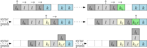
Figure 16: A line $L_{i}$ of agents inside grey cells, with map directions above, pushing and turning through empty and non-empty cells in blue (of label $k$). The green and yellow cells show state swapping.

When $L_{i}$ moves through a series of non-empty cells, it guarantees that they are neither separated or disconnected while pushing. To achieve this, when $l_{t}$ or $k_{l_{t}}$ calls for synchronisation, any line agent $p_{i}$ labelled $l$ whose successor shows a label with star ($k_{l}^{\star}$ or $k_{l}^{\star}c$ ), both swap their states. It continues to swap states forwardly via consecutive non-empty cells until reaches the tail $l_{t}$ or a line agent $l$. Though, when $L_{i}$ traverses entirely through $R$ and reaches the segment tail $s_{t}$, it may find another non-empty cell after swapping states with $s_{t}$. Hence, the same argument above still holds in this case. Figure 18 shows this case.

Figure 17: Four agents in a line inside grey cells swap states with others occupying consecutive yellow cells.

Whenever $L_{i}$ pushes into an empty cell $(x,y)$, it fills $(x,y)$ with an agent $p\in L_{i}$. During pushing, $L_{i}$ always keeps the original position of a non-empty cell and restores it to its initial state (via state swapping). However, there exists a case that may break the connectivity. Consider a line $L_{i}$ pushing along $R$ and turning at a corner agent labelled $k_{l_{t}}c$, which has two diagonal neighbours where both are not adjacent to any line agent, as depicted in Figure 18 top. In this case, when $k_{l_{t}}c$ moves down, it will break connectivity with its upper diagonal neighbour. Hence, the transformation resolves this issue locally depending on the agents’ local view. When $k_{l_{t}}c$ observes a pushing agent and has one or two diagonal neighbours, it temporarily switches to a state that allows it to move one step further while $l_{t}$ updates into a turning agent. This also permits all line agents to turn sequentially until they reach the head $l_{h}$, which turns and waits for $k_{l_{t}}c$ to return to its initial cell. Figure 18 depicts how to handle this situation. Other orientations follow symmetrically by rotating the system $90^{\circ},180^{\circ}$ or $270^{\circ}$ clockwise and counter-clockwise.

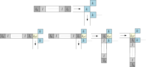
Figure 18: A line $L_{i}$ pushing through a route $R$ turns at a corner agent labelled $k_{l_{t}}c$ that has two diagonal neighbours, neither of which is adjacent to any line agent.

Thus, all agents of $L_{i}$ are labelled and organised in such a way that can transparently push through a route $R$ of any configuration $C_{R}$, whether it is being empty or partially/fully occupied. It implies that $L_{i}$ remains connected when travelling as well as the whole configuration. Further, the original state of $C_{R}$ has been restored and all of its nodes (if any) have been left unchanged. As a result, $L_{i}$ meets all of the transparency criteria of line moves in [3]. ∎

The complexity of Push is provided in the following lemma based on the number of line moves and communication rounds.

Lemma 10

A straight line $L_{i}$ traverses through a route $R$ of any configuration $C_{R}$, taking at most $O(|L_{i}|)$ line moves within $O(|L_{i}|\cdot|R|)$ rounds.

Proof

The bound of moves depends on three factors, the number of empty cells on $R$, the length of $L_{i}$ and the number of turns on $R$. Say that $R$ is free of agents (fully empty) and has at most 3 turns, then $L_{i}$ requires at most $|L_{i}|+3|L_{i}|+|L_{i}|=5|L_{i}|=O(|L_{i}|)$ moves (proved in Lemma 9) to push through $R$. On the other hand, the communication cost of this sub-phase could be very high in the case of a fully occupied route $R$ when individuals perform many functions such as synchronisation, activation, state swapping, and map arrow forwarding. Those actions can be carried either sequentially or concurrently during the transformation and can be analysed independently of each other. In this case, we set an upper bound on the most dominating work.

Assume that $R$ is completely occupied by other agents in the shape (in a worst-case), from the cell adjacent to the line tail $l_{t}$ tp the cell adjacent to $s_{h}$. Then, $l_{t}$ needs to traverse over at most $|R|$ agents in order to arrive at $s_{h}$, which costs $t_{1}^{c}=|R|$ rounds. Further, $l_{t}$ requires a number of synchronisations equal to $|L_{i}|$ to move all line agents along $R$ at a cost of no more than $t_{2}^{c}=|L_{i}|\cdot|R|$ rounds. In each synchronisation, a line agent swaps its state with $|R|$ agents and forwards its map direction over line agents to $l_{t}$ within at most $t_{3}^{c}=|L_{i}|+|R|$ rounds. Thus, this sub-phase results in a maximum number of communications $T^{c}=t_{1}^{c}+t_{2}^{c}+t_{3}^{c}=|R|+(|L_{i}|\cdot|R|)+(|L_{i}|+|R|)=O(L_{i}|\cdot|R|)$ rounds. This bound holds when other agents occupy $|L_{i}|$ consecutive horizontal and vertical cells beyond $s_{h}$. ∎

3.5 Recursive call on the segment $S_{i}$ into a line $L_{i}^{\prime}$

This sub-phase, RecursiveCall, is the heart of this transformation and is recursively called on the next segment $S_{i}$, which eventually transforms into another straight line $L_{i}^{\prime}$ of $2^{i}$ agents.

When a segment tail $s_{t}$ swaps states with $l_{h}$, it accordingly acts as follows: (1) propagates a special mark transmitted along all segment agents towards the head $s_{h}$, (2) deactivates itself by updating label to $c_{1}\leftarrow k$, (3) resets all of its components, except local direction in $c_{4}$. Similarly, once a segment agent $p_{i}$ observes this special mark, it propagates it to its successor $p_{i+1}$, deactivates itself, and keeps its local direction in $c_{4}$ while resetting all other components. When the segment head $s_{h}$ notices this special mark, it changes to a line head state ($c_{1}\leftarrow l_{h}$) and then recursively repeats the whole transformation from round $1$ to $i-1$. Figure 3 presents a graphical illustration of RecursiveCall applied on a diagonal line shape.

3.6 Merge the two lines $L_{i}$ and $L_{i}^{\prime}$

The final sub-phase of this transformation is Merge, which combines two straight lines into a single double-sized line, described as follows. The previous sub-phase, RecursiveCall, transforms the segment $S_{i}$ into a straight line $L_{i}^{\prime}$, starts from a head $l_{h}$ and ends at a tail $l_{t}$. Currently, the tail of $L_{i}^{\prime}$ occupies a cell adjacent to the head of $L_{i}$. Hence, $l_{h}$ can simply check if $L_{i}^{\prime}$ is in line or perpendicular to $L_{i}$ exploiting the previous procedure of CheckSeg. Without loss of generality, say that the tail agent of $L_{i}^{\prime}$ occupies cell $(x,y)$ and $L_{i}$ occupies cells $(x,y),\ldots,(x+|L_{i}|-1,y)$. Then, $L_{i}^{\prime}$ could be either (1) perpendicular with agents occupying $(x,y),\ldots,(x,y+|L_{i}|-1)$ or (2) in line on cells $(x,y),\ldots,(x-|L_{i}|-1,y)$. In (1), $l_{h}$ emits a mark that travels via agents of $L_{i}^{\prime}$ until it reaches the other head, where it asks to change the direction of $L_{i}^{\prime}$, allowing $L_{i}^{\prime}$ and $L_{i}$ to combine into a single straight line $L_{i+1}$ of double length and designate one head and tail for $L_{i+1}$. In (2), $L_{i}^{\prime}$ and $L_{i}$ have already formed $L_{i+1}$; all that remains is to switch and update labels to assign a head $l_{h}$, tail $l_{t}$ and $2^{i+1}$ line agents $l$ in between.

Now, it is sufficient to upper bound this sub-phase by analysing only a worst-case of (1). Obviously, the straight line $L_{i}^{\prime}$ pushes and turns within a distance equal to its length in order to line up with $L_{i}$. It is worth noting that the agents of $L_{i}^{\prime}$ do not require full synchronisation for each push. Instead, they simply need to sync the head and tail of $L_{i}^{\prime}$ where both perform pushing at the same time. When an agent $p_{i}\in L_{i}^{\prime}$ turns, it tells its predecessor $p_{i-1}\in L_{i}^{\prime}$ to turn too. Hence, the total number of moves is at most $O(|L_{i}^{\prime}|)$. The communication cost splits into: (1) A special mark from $l_{h}$ traverses across $L_{i}^{\prime}$ in $O(|L_{i}^{\prime}|)$ rounds. (2) All agents of $L_{i}^{\prime}$ synchronise in $O(|L_{i}^{\prime}|)$ rounds. (3) Label swapping costs at most $|L_{i}^{\prime}|+|L_{i}|=O(|L_{i}^{\prime}|)$. Therefore, all agents in Merge communicate in linear time, and then we can say:

Lemma 11

An execution of Merge requires at most $O(|L_{i}|)$ line moves and $O(|L_{i}|)$ rounds of communication.

Finally, we analyse the recursion in a worst-case shape in which individuals consume their maximum energy to communicate and move. The runtime is based on the analysis of the centralised version that has been proved in Section LABEL:sec:Hamiltonianshapes. Let $T_{i}^{c}$ and $T_{i}^{m}$ denote the total number of communication rounds and moves in phase $i$, respectively, for all $i\in{1,\ldots,\log n}$. Apart from RecursiveCall, the $2^{i}$ agents forming a straight line $L_{i}$ in phase $i$ go through DefineSeg, CheckSeg, DrawMap, Push and Merge sub-phases that take total parallel rounds of communication $t^{c}_{i}$ at most:

$$t^{c}_{i}=(4\cdot|L_{i}|)+(|L_{i}|\cdot|R|)\approx O(|L_{i}|\cdot|L_{i}|).$$

Then, in Push and Merge sub-phases, the line $L_{i}$ traverses along a route of total movements $t^{m}_{i}$ in at most:

$$t^{m}_{i}=|L_{i}|+|L_{i}^{\prime}|=O(|L_{i}|).$$

Now, let $T^{c}_{i-1}$ denote a total number of parallel rounds required for a recursive call of RecursiveCall on $2^{i}$ agents of the segment $S_{i}$, which transforms into another straight line $L^{\prime}_{i}$. Given $|L_{i}|=2^{i}$, this recursion in phase $i$ costs a total rounds bounded by:

$$T^{c}_{i} \leq i\cdot(|L_{i}|\cdot|L_{i}|)\leq i\cdot(2^{i})^{2}$$

$$T^{c}_{i} O(\leq i\cdot n^{2}).$$

Thus, we conclude that the call of RecursiveCall in the final phase $i=\log n$ requires a total rounds $T^{c}_{\log n}$:

$$T^{c}_{\log n} \leq n^{2}\cdot\log n$$

$$=O(n^{2}\log n).$$

The same argument follows on the total number of movements $T^{c}_{i-1}$ for a recursive call of RecursiveCall, which costs at most:

$$T^{m}_{i} \leq i\cdot|L_{i}|\leq i\cdot(2^{i})$$

$$T^{m}_{i} \leq O(\leq i\cdot n).$$

Finally, by the final phase $i=\log n$, all agents in the system pushes a total number of moves $T^{m}_{\log n}$ that bounded by:

$$T^{m}_{\log n} \leq n\cdot\log n$$

$$=O(n\log n).$$

Overall, given a Hamiltonian path in an initial connected shape $S_{I}$ of individuals of limited knowledge and permissible line moves, the following lemma states $S_{I}$ can be transformed into a straight line $S_{L}$ in a number of moves that match the optimal centralised transformation fulfilling the connectivity-preserving condition.

Lemma 12

Given an initial Hamiltonian shape $S_{I}$ of $n$ agents, this strategy transforms $S_{I}$ into a straight line $S_{L}$ of the same order in $O(n\log n)$ line moves and $O(n^{2}\log n)$ rounds, while preserving connectivity during transformation.

Thus, we can finally provide the following theorem:

Theorem 3.1

The above distributed transformation solves HamiltonianLine and takes at most $O(n\log_{2}n)$ line moves and $O(n^{2}\log_{2}n)$ rounds.

References

- [1] Adleman, L.M.: Molecular computation of solutions to combinatorial problems. Science 266(11), 1021–1024 (1994)
- [2] Akitaya, H.A., Arkin, E.M., Damian, M., Demaine, E.D., Dujmović, V., Flatland, R., Korman, M., Palop, B., Parada, I., van Renssen, A., et al.: Universal reconfiguration of facet-connected modular robots by pivots: the o (1) musketeers. Algorithmica 83(5), 1316–1351 (2021)
- [3] Almethen, A., Michail, O., Potapov, I.: On efficient connectivity-preserving transformations in a grid. In: Algorithms for Sensor Systems - 16th International Symposium on Algorithms and Experiments for Wireless Sensor Networks, ALGOSENSORS. vol. 12503, pp. 76–91 (2020)
- [4] Almethen, A., Michail, O., Potapov, I.: Pushing lines helps: Efficient universal centralised transformations for programmable matter. Theoretical Computer Science 830-831, 43 – 59 (2020)
- [5] Aloupis, G., Benbernou, N., Damian, M., Demaine, E., Flatland, R., Iacono, J., Wuhrer, S.: Efficient reconfiguration of lattice-based modular robots. Computational geometry 46(8), 917–928 (2013)
- [6] Aloupis, G., Collette, S., Demaine, E., Langerman, S., Sacristán, V., Wuhrer, S.: Reconfiguration of cube-style modular robots using O(logn) parallel moves. In: International Symposium on Algorithms and Computation. pp. 342–353. Springer (2008)
- [7] Angluin, D., Aspnes, J., Diamadi, Z., Fischer, M., Peralta, R.: Computation in networks of passively mobile finite-state sensors. Distributed Computing 18(4), 235–253 (2006)
- [8] Boneh, D., Dunworth, C., Lipton, R.J., Sgall, J.: On the computational power of dna. Discrete Applied Mathematics 71(1-3), 79–94 (1996)
- [9] Bourgeois, J., Goldstein, S.: Distributed intelligent MEMS: progresses and perspective. IEEE Systems Journal 9(3), 1057–1068 (2015)
- [10] Czyzowicz, J., Dereniowski, D., Pelc, A.: Building a nest by an automaton. Algorithmica 83(1), 144–176 (2021)
- [11] Daymude, J., Derakhshandeh, Z., Gmyr, R., Porter, A., Richa, A., Scheideler, C., Strothmann, T.: On the runtime of universal coating for programmable matter. Natural Computing 17(1), 81–96 (2018)
- [12] Derakhshandeh, Z., Gmyr, R., Porter, A., Richa, A., Scheideler, C., Strothmann, T.: On the runtime of universal coating for programmable matter. In: International Conference on DNA-Based Computers. pp. 148–164. Springer (2016)
- [13] Derakhshandeh, Z., Gmyr, R., Richa, A., Scheideler, C., Strothmann, T.: Universal shape formation for programmable matter. In: Proceedings of the 28th ACM Symposium on Parallelism in Algorithms and Architectures. pp. 289–299. ACM (2016)
- [14] Di Luna, G.A., Flocchini, P., Santoro, N., Viglietta, G., Yamauchi, Y.: Shape formation by programmable particles. Distributed Computing (Mar 2019)
- [15] Doty, D.: Theory of algorithmic self-assembly. Communications of the ACM 55, 78–88 (2012)
- [16] Douglas, S., Dietz, H., Liedl, T., Högberg, B., Graf, F., Shih, W.: Self-assembly of dna into nanoscale three-dimensional shapes. Nature 459(7245), 414 (2009)
- [17] Dumitrescu, A., Pach, J.: Pushing squares around. In: Proceedings of the twentieth annual symposium on Computational geometry. pp. 116–123. ACM (2004)
- [18] Dumitrescu, A., Suzuki, I., Yamashita, M.: Formations for fast locomotion of metamorphic robotic systems. The International Journal of Robotics Research 23(6), 583–593 (2004)
- [19] Dumitrescu, A., Suzuki, I., Yamashita, M.: Motion planning for metamorphic systems: Feasibility, decidability, and distributed reconfiguration. IEEE Transactions on Robotics and Automation 20(3), 409–418 (2004)
- [20] Fekete, S.P., Gmyr, R., Hugo, S., Keldenich, P., Scheffer, C., Schmidt, A.: Cadbots: Algorithmic aspects of manipulating programmable matter with finite automata. Algorithmica 83(1), 387–412 (2021)
- [21] Flocchini, P., Prencipe, G., Santoro, N.: Distributed computing by oblivious mobile robots. Synthesis Lectures on Distributed Computing Theory 3(2), 1–185 (2012)
- [22] Fukuda, T.: Self organizing robots based on cell structures-cebot. In: Proc. IEEE Int. Workshop on Intelligent Robots and Systems (IROS’88). pp. 145–150 (1988)
- [23] Gilpin, K., Knaian, A., Rus, D.: Robot pebbles: One centimeter modules for programmable matter through self-disassembly. In: Robotics and Automation (ICRA), 2010 IEEE International Conference on. pp. 2485–2492. IEEE (2010)
- [24] Gmyr, R., Hinnenthal, K., Kostitsyna, I., Kuhn, F., Rudolph, D., Scheideler, C., Strothmann, T.: Forming tile shapes with simple robots. Natural Computing pp. 1–16 (2019)
- [25] Itai, A., Papadimitriou, C., Szwarcfiter, J.: Hamilton paths in grid graphs. SIAM Journal on Computing 11(4), 676–686 (1982)
- [26] Knaian, A., Cheung, K., Lobovsky, M., Oines, A., Schmidt-Neilsen, P., Gershenfeld, N.: The milli-motein: A self-folding chain of programmable matter with a one centimeter module pitch. In: 2012 IEEE/RSJ International Conference on Intelligent Robots and Systems. pp. 1447–1453. IEEE (2012)
- [27] Michail, O., Skretas, G., Spirakis, P.: On the transformation capability of feasible mechanisms for programmable matter. Journal of Computer and System Sciences 102, 18–39 (2019)
- [28] Michail, O., Spirakis, P.: Simple and efficient local codes for distributed stable network construction. Distributed Computing 29(3), 207–237 (2016)
- [29] Michail, O., Spirakis, P.: Elements of the theory of dynamic networks. Commun. ACM 61(2), 72–81 (2018)
- [30] Minsky, M.L.: Computation. Prentice-Hall Englewood Cliffs (1967)
- [31] Nguyen, A., Guibas, L., Yim, M.: Controlled module density helps reconfiguration planning. In: Proc. of 4th International Workshop on Algorithmic Foundations of Robotics. pp. 23–36 (2000)
- [32] Prakash, V.P., Patvardhan, C., Srivastav, A.: Effective heuristics for the bi-objective euclidean bounded diameter minimum spanning tree problem. In: International Conference on Next Generation Computing Technologies. pp. 580–589. Springer (2017)
- [33] Rothemund, P.: Folding dna to create nanoscale shapes and patterns. Nature 440(7082), 297–302 (2006)
- [34] Rothemund, P., Winfree, E.: The program-size complexity of self-assembled squares. In: Proceedings of the 32nd annual ACM symposium on Theory of computing (STOC). pp. 459–468. ACM (2000)
- [35] Rubenstein, M., Cornejo, A., Nagpal, R.: Programmable self-assembly in a thousand-robot swarm. Science 345(6198), 795–799 (2014)
- [36] Toffoli, T., Margolus, N.: Programmable matter: concepts and realization. Physica. D, Nonlinear phenomena 47(1-2), 263–272 (1991)
- [37] Walter, J., Welch, J., Amato, N.: Distributed reconfiguration of metamorphic robot chains. Distributed Computing 17(2), 171–189 (2004)
- [38] Winfree, E.: Algorithmic Self-Assembly of DNA. Ph.D. thesis, California Institute of Technology (1998)
- [39] Woods, D., Chen, H., Goodfriend, S., Dabby, N., Winfree, E., Yin, P.: Active self-assembly of algorithmic shapes and patterns in polylogarithmic time. In: Proceedings of the 4th conference on Innovations in Theoretical Computer Science. pp. 353–354. ACM (2013)
- [40] Yamashita, M., Suzuki, I.: Characterizing geometric patterns formable by oblivious anonymous mobile robots. Theoretical Computer Science 411(26-28), 2433–2453 (2010)
- [41] Yim, M., Shen, W., Salemi, B., Rus, D., Moll, M., Lipson, H., Klavins, E., Chirikjian, G.: Modular self-reconfigurable robot systems [grand challenges of robotics]. IEEE Robotics & Automation Magazine 14(1), 43–52 (2007)