Neural TMDlayer: Modeling Instantaneous flow of features via SDE Generators

Abstract

We study how stochastic differential equation (SDE) based ideas can inspire new modifications to existing algorithms for a set of problems in computer vision. Loosely speaking, our formulation is related to both explicit and implicit strategies for data augmentation and group equivariance, but is derived from new results in the SDE literature on estimating infinitesimal generators of a class of stochastic processes. If and when there is nominal agreement between the needs of an application/task and the inherent properties and behavior of the types of processes that we can efficiently handle, we obtain a very simple and efficient plug-in layer that can be incorporated within any existing network architecture, with minimal modification and only a few additional parameters. We show promising experiments on a number of vision tasks including few shot learning, point cloud transformers and deep variational segmentation obtaining efficiency or performance improvements.

1 Introduction

Consider a deep neural network model with parameters $W$ which we train using the following update rule,

$$W\leftarrow W-\eta\nabla_{W}\mathbb{E}_{z}R\left(W,z\right)$$ (1)

where $z$ is a random variable representing data and $R(\cdot)$ represents the loss function. Now, consider a slightly general form of the same update formula,

$$W\leftarrow W-\eta\nabla_{W}\mathbb{E}_{z}R\left(W,{\color[rgb]{0,0,1}T}z\right).$$ (2)

The only change here is the introduction of $T$ which can be assumed to be some data transformation matrix. If $T=I$, we see that Stochastic Gradient Descent (SGD) is a special case of (2) under the assumption that we approximate the expectation in (2) with finite iid samples (or a mini-batch).

Let us unpack the data transformation notation a bit to check what it offers. If a set of transformations $T$ are chosen beforehand, and applied to the data samples before training commences, $Tz$ simply represents data samples derived via data augmentation. On the other hand, $Tz$ may not necessarily be explicitly instantiated as above. For example, spherical CNN [16] shows that when point cloud type data are embedded on the sphere with spherical convolutional operators, then it is possible to learn representations of data that are equivariant to the group action of rotations with no explicit data augmentation procedure. In particular, these approaches register each data point on a standard template (like the sphere) on which efficient convolutions can be defined based on differential geometric constructions – in other words, utilizing the properties of the transformations $T$ of interest and how they relate the data points, such a treatment enables the updates to implicitly take into account the loss on $Tz$. Conceptually, many results [16, 48, 42] on equivariance show that by considering the entire orbit of each sample (a 3D point cloud) during training, for special types of $T$, it is possible to avoid explicit data augmentation.

We can take a more expanded view of the above idea. Repeated application of a transformation $T$ on data point $z$ produces a discrete sequence $\{z(t)\}_{t=0}^{\infty}$ where $z(0)=z,z(t)=T^{t-1}z$. In general, the transformation matrix at the $t$-th step, denoted by $T(t)$, need not even be generated from a fixed matrix. Indeed, in practice $T(t)$ is selected from a set of appropriate transformations such as rotation, blur and so on, with some ordering, which could even be stochastic. At a high level, approaches such as [16, 12] can be seen as a special case of (2). Making this argument precise needs adding an appropriate number of auxiliary variables and by averaging over all possible realizable $T$’s – the specific steps are not particularly relevant since apart from helping set up the intuition we just described, algorithms for equivariance to specific group actions do not directly inform our development. For the sake of convenience, we will primarily focus on the continuous time system since under the same initial conditions, the trajectories of both (continuous and discrete) systems coincide at all integers $t$.

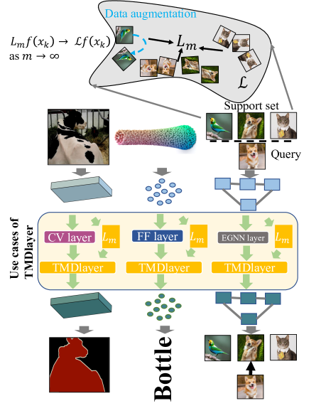
Figure 1: Overview of TMDlayer use in few-shot recognition, point cloud learning and segmentation. “EGNN” refers to edge-labeling graph neural network [25]; “FF” refers to feed-forward layer (10) and “CV” refers to our proposed deep Chan Vese model (12). The manifold (top) describes the meaning of $\mathcal{L}$ and $L_{m}$: $\mathcal{L}$ captures the structure of the manifold. $L_{m}$ is an approximation of $\mathcal{L}$ constructed from samples.

What does $z(t)$ actually represent? There are two interpretations of $z(t)$: (i) it formalizes on-the-fly or instantaneous (smooth) data augmentation which are often used to accelerate training by exploiting symmetries in the landscape of $R$, and (ii) a data dependent $T$ can be designed for invariance-like requirements, useful for downstream applications. In fact, learning data dependent transformations has also been explored by [14]. The starting point of this work is to exploit the view that the data sample provided to us is merely a snapshot of an underlying process which we will discuss shortly. Nonetheless, the key hypothesis is that specifying this process to our deep neural network model will be beneficial and provide a fresh perspective on some strategies that are already in use in the literature.

Main ideas. The foregoing use of “process” to describe the data sample hints at the potential use of an ordinary differential equations (ODE). While ODE type constructions can be used to characterize simple processes, it will be insufficient to model more complex processes that will better reflect practical considerations. The key challenge in directly instantiating the “$z(t)$” idea for SDEs is that it is clearly infeasible since there are infinite possible trajectories for the same initial conditions. Our main insight is that recent results in the SDE literature show that (under some technical conditions), the dynamics $z(t)$ can be completely characterized by (functions of) the infinitesimal generator $\mathcal{L}$ of the process $z(t)$ which can be efficiently estimated using finite data. We exploit this result via a simple modification to the estimation procedure – one that can be directly used within any backpropagation based training scheme. Specifically, we exploit the result from [2] where the authors call the generator Target Measure Diffusion map (TMDmap). This leads to our TMDlayer that can be conveniently dropped into a network, and be used as a plug-and-play module with just a few additional parameters. When utilized within standard deep learning pipelines, our layer allows incorporating much richer domain information if available, or as a regularizer or an augmentation scheme, or as a substitute to an existing layer. We find this is beneficial to the overall performance of the model.

Our contributions. Models such as a Neural ODE [10] and Neural SDE [34] usually parameterize the dynamical system as a stand-alone model, and show how gradients can be efficiently backpropagated through this module. We take a different line of approach: we propose a stochastic process inspired layer which, in its most rudimentary form, can be thought of as an augmentation scheme that can work with existing layers in deep neural networks. But different from explicit data augmentation (rotation, flipping) that happens in the input image space, our layer can be utilized in the feature space and is fully adaptive to the input. But it is more than another augmentation scheme. Our layer allows modeling the time varying/stochastic property of the data/features, and controls them by a proper parameterization which is highly parameter efficient. We show that this stochasticity is not only mathematically interesting, but can be exploited in applications including point cloud transformers, object segmentation and few-shot recognition.

1.1 Related Work.

Early work in vision has made extensive use of differential equations [7, 36, 45, 6], especially for segmentation. In machine learning, differential equations are useful for manifold learning [3] and semi-supervised learning [4, 38] among others. Recently, a number of strategies combine differential equations with deep neural networks (DNNs) for solving vision problems. For example, [9] utilizes a conditional random field after the CNN encoder to refine the semantic segmentation results whose update rules can be viewed as a differential equation and [37, 22] uses a CNN to extract visual features before feeding them to an active contour model which iteratively refines the contour according to the differential equation. Separately, the literature includes strategies for solving differential equations with DNNs [24, 39, 32]. Over the last few years, a number of formulations including neural ODE [10], neural SDE [34] and augmented neural ODE [15] have been proposed, motivated by the need to solve differential equation modules within DNNs. Note that [34] proposes to stabilize the neural ODE network with stochastic noise, which leads to a neural SDE, a setting quite different from the one studied here. Finally, we note that SDEs as a tool have also been used for stochastic analysis of DNNs [8].

2 Preliminaries

Background. Partial differential equation (PDE) is a functional equation in which the solution satisfies given relations between its various partial derivatives interpreted as multivariable functions. Consider a commonly used PDE model for segmentation – the heat equation,$\frac{\partial u}{\partial t}=\Delta u,$ where $u$ depends on both $X$ and $t$. By the celebrated Feynman-Kac formula, we know that the solution $u$ can be equivalently written as a conditional expectation with respect to a continuous time stochastic process $X_{t}$. This means that the solution (segmentation) $u$ can be obtained by averaging a sequence of stochastic integration problems. For prediction, we need an algebraic concept called the “generator” of a function (like a neural network) since we are more interested in the pushforward mappings $f\left(X_{t}\right)$.

Given a time invariant stochastic process $X_{t}$, the (infinitesimal) generator $\mathcal{L}$ of a function $f$ is defined as,

$$\mathcal{L}f(X):=\lim\limits_{t\to 0}\frac{\mathbb{E}\left[f(X_{t})\right]-f(X_{0})}{t}.$$ (3)

If the process $X_{t}$ is deterministic, the expectation operator $\mathbb{E}$ becomes identity, and so the generator $\mathcal{L}$ simply measures the instantaneous rate of change in $f$ with respect to $X$. In addition, say that $X_{t}$ can also be expressed as a (Itô) Stochastic Differential Equation (SDE), i.e., $X_{t}$ satisfies:

$$dX_{t}=b(X_{t})dt+\sigma(X_{t})dW_{t},$$ (4)

where $W_{t}$ is a (multidimensional) Brownian motion with covariance $C$, and $b,\sigma$ represent drift and diffusion functions. Then, it turns out that $\mathcal{L}$ can be written in closed form (without limit) as,

$$\mathcal{L}f=b\cdot\nabla f+\sigma C\sigma^{T}\cdot\nabla^{2}f,$$ (5)

where $\mathcal{L}$ acts as a linear operator on functions $f$, see [29]. We will shortly explain how to estimate and utilize $\mathcal{L}$.

Setup. Consider the setting where $X$ represents our input features (say, an image as a 3D array for the RGB channels) and $f$ is a network with $L$ layers. Let the data be in the form of points $\mathcal{D}^{(m)}:={x_{1},x_{2},...,x_{m}}\in\mathcal{R}^{N}$ with $N>0$, which lie on a compact $d$-dimensional differentiable submanifold $\mathcal{M}\subseteq\mathcal{R}^{N}$ which is assumed to be unknown. We assume that $f$ in our case is defined implicitly using samples $x_{i}\in\mathcal{M}$, and so it is impossible to obtain closed form expressions for the operators $\nabla,\nabla^{2}$ in (5). In such cases, recall that, when $\sigma\equiv 0$, Diffusion maps [13] uncovers the geometric structure $\mathcal{M}$ by using $\mathcal{D}^{(m)}$ to construct an $m\times m$ matrix $L_{m}$ as an approximation of the linear operator $\mathcal{L}$.

Interpreting SDE. Recall that when $\mathcal{L}$ is used on the input space, it can model stochastic transformations to the input image (rotation and clipping are special cases). When $\mathcal{L}$ is used on the feature space (e.g., in an intermediate layer of a DNN), it can then model stochastic transformations of the features where it is hard to hand design augmentation methods. Moreover, it enables us to parameterize and learn the underlying stochastic changes/SDE of the features.

Roadmap. In the next section, we describe the estimation of differential operator $\mathcal{L}$ within deep network training pipelines. Based on this estimate, we define TMDlayer as a approximation to $f(X_{\Delta t}):=f(X,\Delta t)$ for a small time interval $\Delta t$ using Taylor’s theorem. In §4, we discuss four different applications of TMDlayer, where the pushforward measure $f(X,\Delta t)$ under the flow of features (interpreted as a vector field) $f(X,0)$ may be a reasonable choice.

3 Approximating $\mathcal{L}$ in Feedforward Networks

We now discuss a recently proposed nonparametric procedure to estimate $L_{m}$ given finite samples $x$ when $\sigma\not\equiv 0$. This is an important ingredient because in our setup, we often do not have a meaningful model of minibatch samples, especially in the high dimensional setting (e.g., images).

Constructing $L_{m}$ in DNN training. The definition in (3) while intuitive, is not immediately useful for computational purposes. Under some technical conditions such as smoothness of $b,\sigma,f$, and the rank of $C$, [2] recently showed that for processes that satisfy (4), it is indeed possible to construct finite sample estimators $L_{m}$ of $\mathcal{L}$. In [2], the approach is called Target Measure Diffusion (TMD) so we call our proposed layer, a TMDlayer.

To construct the differential operator, we first need to compute a kernel matrix $K\in R^{m\times m}$ from the data. For problems involving a graph or a set of points as input, we can simply use the given data points ($m$ would be the number of nodes in the graph, or the number of points in the set), while for problems with a single input (e.g., standard image classification), we may not have access to $m$ data points directly. In this case, we can construct the kernel matrix by sampling a batch from the dataset and processing them together because we can often assume that the entire dataset is, in fact, sampled from some underlying distribution.

1 Input: Function $f$, a batch of data samples $X=\{x_{1},...,x_{m}\}$, coefficient $\epsilon$, parameterized time interval $\Delta t$

2 Construct distance matrix $K_{\epsilon}$ by (6)

3 Compute kernel density estimate: $q_{\epsilon}(x_{i})=\sum_{j=1}^{m}(K_{\epsilon})_{ij}$

4 Parameterize target distribution by (7)

5 Form the diagonal matrix $D_{\epsilon,\pi}$ with components $(D_{\epsilon,\pi})_{ii}=\pi^{1/2}(x_{i})q^{-1}_{\epsilon}(x_{i})$

6 Use $D_{\epsilon,\pi}$ to right-normalize $K_{\epsilon}$: $K_{\epsilon,\pi}=K_{\epsilon}D_{\epsilon_{\pi}}$

7 Construct $L_{m}$ by (8) using $(\tilde{D}_{\epsilon,\pi})_{ii}:=\sum_{j=1}^{m}(K_{\epsilon,\pi})_{ij}$

Return: $f(X)+\Delta t\cdot L_{m}f(X)$

Algorithm 1 Operational steps in TMDlayer

After getting the set of data samples, we first project the data into a latent space $\mathbb{R}^{h}$ with a suitable $h$ using a learnable linear layer, before evaluating them with an appropriate kernel function such as,

$$k_{\epsilon}(x,y)=\exp(-(4\epsilon)^{-1}\|x-y\|^{2}).$$ (6)

We then follow [2] to construct the differential operator $\mathcal{L}$ as follows: we compute the kernel density estimate $q_{\epsilon}(x_{i})=\sum_{j=1}^{m}(K_{\epsilon})_{ij}$. Then, we form the diagonal matrix $D_{\epsilon,\pi}$ with components $(D_{\epsilon,\pi})_{ii}=\pi^{(1/2)}(x_{i})q_{\epsilon}^{-1}(x_{i})$. Here, we allow the network to learn $\pi$ by

$$\pi^{1/2}(x_{i})=g(x_{i}),$$ (7)

where $g$ can be a linear layer or a MLP depending on the specific application. Next we use $D_{\epsilon,\pi}$ to right-normalize the kernel matrix $K_{\epsilon,\pi}=K_{\epsilon}D_{\epsilon,\pi}$ and use $\tilde{D}_{\epsilon,\pi}$ which is the diagonal matrix of row sums of $K_{\epsilon,\pi}$ to left-normalize $K_{\epsilon,\pi}$. Then we can build the TMDmap operator as

$$L_{m}=\epsilon^{-1}(\tilde{D}_{\epsilon,\pi}^{-1}K_{\epsilon,\pi}-I).$$ (8)

We will use (8) to form our TMDlayer as described next.

3.1 TMDlayer: A Transductive Correction via $L_{m}$

Observe that (4) is very general and can represent many computer vision tasks where the density $\pi$ could be defined using a problem specific energy function, and $W_{t}$ is the source of noise. In other words, we aim to capture the underlying structure of the so-called image manifold [61] by using its corresponding differential operator (5). Intuitively, this means that if we are provided a network $f_{W}$ with parameters $W$, then by Taylor’s theorem, the infinitesimal generator estimate $L_{m}$ can be used to approximate the change of $f_{W}$ as follows:

$$\mathbb{E}_{x}f_{W}(x,\Delta t)\approx f_{W}(x,0)+\Delta t\cdot{L}_{m}[f_{W}],$$ (9)

where $[f_{W}]\in\mathbb{R}^{m}$ such that the $i-$th coordinate $[f_{W}]_{i}=f_{W}(x_{i})$, and $\Delta t$ is interpreted as a hyperparameter in our use cases, see Algorithm 1.

Inference using $L_{m}$. In the ERM framework, typically, each test sample is used independently, and identically i.e., network (at optimal parameters) is used in a sequential manner for predictive purposes. Our framework allows us to further use relationships between the test samples for prediction. In particular, we can design custom choices of $b,\sigma$ tailored for downstream applications. For example, in applications that require robustness to small and structured perturbations, it may be natural to consider low bias diffusion processes i.e., we can prescribe the magnitude using $\|b\|_{p}\leq\kappa$ almost everywhere for some small constant $\kappa>0$ (akin to radius of perturbation) and structure using diffusion functions $\sigma,C$. Inference can then be performed using generators $\mathcal{L}$ derived using the corresponding process.

Layerwise $\mathcal{L}$ for improved estimation of $L_{m}$. While (9) allows us to use $L_{m}$ for any network with no modifications, using it naively can be unsatisfactory in practice. For example, often we find that features from input layers might not be too informative for the task and may hinder training, especially in the early stages. We suggest a simple adjustment: instead of applying approximation in (9) on the entire network, we do it layerwise – this could be every intermediate layer or several layers of interest. It means that $f$ can in principle be any layer (e.g., a layer in graph neural networks or a layer in Resnet), as shown in Fig. 1.

Justification. Recall that most feed-forward neural networks can be completely defined by a finite sequence of linear transformations followed by activation functions (along with intermediate normalization layers). One option is to estimate $L_{m}$ by directly applying the Taylor series-like expansion in (9) on $f=f^{l}\circ f^{l-1}\circ\cdots f^{1}$ where $l$ represents the number of layers. However, from (9) we can see that the variance of such an estimate of the value $L_{m}[f_{W}]$ will be high due to the well-known propagation of uncertainty phenomenon (across $f^{i}$’s). To avoid this, we can estimate $L_{m}[f_{W}]$ in a sequential manner i.e., use $L_{m}[f^{i-1}_{W}]$ to estimate $L_{m}[f^{i}_{W}]~{}\forall~{}i\in[l]$. We will show in §4 that this parameterization can be useful in various applications.

Synopsis. We briefly summarize the benefits of our TMDlayer next: (i) Our TMDlayer can parameterize the underlying stochastic transformations of features, providing a way to augment features at any layer. (ii) The stochasticity/randomness in our TMDlayer is a stability inducing operation for robust predictive purposes [20]. (iii) Our TMDlayer is parameter efficient. All we need is a projection linear layer $h$ and a linear layer $g$ parameterizing the density $\pi$ and a scalar parameter $\Delta t$. In practice, we can work with a small latent dimension (e.g., $h$ = 16) when constructing $L_{m}$, thus the total number of parameters in TMDlayer is very small when compared with the layer function $f$ in most deep learning applications. But the reader will see that a mild limitation of the SDE perspective in practice is that, in principle, the dynamics may eventually get stuck in a meta-stable state. This means that in this case, the estimate $L_{m}$ will not be very informative in the forward pass, and so the gradient estimates might be biased. In such cases, it may be useful to add points by sampling on the orbit if needed. We will now describe four different vision settings where our TMDlayer can be instantiated in a plug-and-play manner.

4 Applications

In this section, we evaluate our TMDlayer in the context of different applications. As a warm-up, in §4.1, we demonstrate the use of TMDlayer on a simple image classification task. We study its properties in both inductive and transductive settings. Then, in §4.2, we move to learning with point cloud datasets. Here, we see that the data type naturally offers a suitable object for leveraging the features of TMDlayer. In this case, we conduct experiments in an inductive setting. Next, in §4.3, we explore the use of TMDlayer on a segmentation task (also in an inductive setting). We propose a novel deep active contour model which can be viewed as a dynamical process within a neural network. We demonstrate the use of our TMDlayer on top of such a dynamical process. Finally, in §4.4, we investigate few-shot learning. Here, the problem setup natively provides the graph needed for computing our $L_{m}$ and allows transductive inference.

4.1 A Simple Sanity check on Resnet

We start with a simple example of image classification on CIFAR10 [28] using Resnet [23], to demonstrate applicability of our TMDlayer and evaluate its behavior.

4.1.1 Role of TMDlayer: Finetuning/Robustify Resnet

We choose Resnet-18 as the backbone network and simply treat each of its three residual blocks Res as $f$ (see [23] for details of a residual block) in TMDlayer as follows,

$$f(x^{l-1})=\text{Res}(x^{l-1})\implies x^{l}=f(x^{l-1})+\Delta t\cdot L_{m}f(x^{l-1}),$$

where $x^{l}$ is the feature at the $l$-th layer and $L_{m}$ is constructed from a mini-batch of samples.

4.1.2 Experimental results

During training, we first sample $m$ data points in a batch and use it as the input so that we can construct $L_{m}$. During test time, an input batch also contains $m$ samples (similar to training time), where $m$ increases from $1$ to $200$. We can see from Table 1 that $m$ does have an influence on the test accuracy where a larger $m$ performs better than a smaller $m$. A key reason is that $L_{m}$ using a larger $m$ can better capture the geometric structure of the data.

We also test whether our TMDlayer can help improve the robustness of the network. We can assess this property by adding random noise to the input image and evaluating the test accuracy (see Table 2). With our TMDlayer, the network is more noise resilient. This can be partly attributed to the use of our parameterized $\Delta t$, which allows the network to control the stochastic process in the TMDlayer adaptively and dependent on the input. In summary, the performance profile is similar (Tab. 1) with small improvements in robustness (Tab. 2).

$m$	Inference w/ TMDlayer	Accuracy (%)
1	No	75.15
1	Yes	87.35
10	Yes	87.65
50	Yes	88.14
100	Yes	88.52
150	Yes	88.55
200	Yes	88.25

Table 1: Accuracy on test set of CIFAR10 after adding TMDlayer to Resnet-18. Here, $m$ is the batch size used to construct $L_{m}$ during test/inference time. The accuracy of Resnet-18 (trained/tested without TMDlayer) is $88.27\%$ comparable to $m\in\{50,100,150\}$.

$\sigma$	0.01	0.02	0.03	0.05	0.1
Resnet-18	87.54	83.90	75.85	53.87	17.27
Ours	87.79	84.37	77.96	56.18	19.18

Table 2: Accuracy on CIFAR10 when adding random noise (mean = $0$, std = $\sigma$) to the input. “Ours” refers to Resnet-18 plus the TMDlayer.

4.2 Point cloud transformer

Tasks involving learning with point cloud data is important within 3D vision. The input here is usually a 3D point cloud represented by a set of points, each associated with its own feature descriptor. These points can be naturally thought of as samples from the underlying distribution which captures the geometric structure of the object. The problem provides an ideal sandbox to study the effect of our TMDlayer. But before we do so, we provide some context for where and how the TMDlayer will be instantiated. Recently, [19] proposed a transformer based model for point cloud learning which achieves state-of-the-art performance on this task – and corresponds to an effective and creative use of transformers in this setting. Nonetheless, Transformer models are known to be parameter costly (e.g., see [5, 56, 59] for cheaper approximations effective in NLP settings) and it is sensible to check to what extent our TMDlayer operating on a simple linear layer can be competitive with the transformer layer proposed in [19]. Our goal will be to check if significant parameter efficiency is possible.

4.2.1 Problem formulation

Denote an input point cloud $\mathcal{P}\in R^{N\times d}$ with $N$ points, each with a $d$-dimensional feature descriptor. The classification task is to predict a class or label for the entire point cloud.

4.2.2 Role of TMDlayer: Replace transformer layer

The point cloud transformer layer in [19] is constructed as,

$$F_{out}=FF(F_{in}-F_{sa})+F_{in},$$ (10)

where FF refers to their feed-forward layer (a combination of Linear, BatchNorm and ReLU layer), and $F_{sa}$ is the output of self-attention module which takes $F_{in}$ as an input (we refer the reader to [19] for more details of their network design, also included in our appendix).

A Transformer layer is effective for point cloud because it simultaneously captures the relation between features of all points. Since our TMDlayer can be viewed as a diffusion operator which captures the structure of the underlying data manifold from the data, we can check to what extent its ability suffices. We use the TMDlayer on a single feed-forward layer to replace the Transformer layer in (10).

$$F_{out}=FF(F_{in})+\Delta t\cdot L_{m}FF(F_{in}).$$ (11)

Surprisingly, it turns out that this simple layer can perform comparably with the carefully designed Transformer layer in (10) while offering a much more favorable parameter efficiency profile. Here, $L_{m}$ is constructed using points of the same point cloud (setting is identical to baselines).

4.2.3 Experimental results

Dataset. We follow [19] to conduct a point cloud classification experiment on ModelNet40 [54]. The dataset contains $12311$ CAD models in $40$ object categories, widely used in benchmarking point cloud shape classification methods. We use the official splits for training/evaluation.

Network architecture and training details. We use the same network as [19] except that we replace each point cloud transformer layer with a TMDlayer built on a single feed forward layer. We follow [19] to use the same sampling strategy to uniformly sample each object via $1024$ points and the same data augmentation strategy during training. The mini-batch size is $32$ and we train $250$ epochs using SGD (momentum $0.9$, initial learning rate $0.01$, cosine annealing schedule). The hidden dimension is $256$ for the whole network and $16$ for constructing $L_{m}$ (in TMDlayer).

Results. We see from Table 3 that our approach achieves comparable performance with [19]. In terms of the number of parameters, using hidden dimension $256$ (used in this experiment) as an example, one self-attention layer contains $148$k parameters; one linear layer contains $65.5$k parameters; and the TMDlayer module only needs $4$k parameters.

Method	Input	#Points	Accuracy(%)
PointNet [41]	P	1k	89.2
A-SCN [55]	P	1k	89.8
SO-Net [31]	P, N	2k	90.9
Kd-Net [26]	P	32k	91.8
PointNet++ [41]	P	1k	90.7
PointNet++ [41]	P, N	5k	91.9
PointGrid [30]	P	1k	92.0
PCNN [1]	P	1k	92.3
PointConv [53]	P, N	1k	92.5
A-CNN [27]	P, N	1k	92.6
DGCNN [52]	P	1k	92.9
PCT [19]	P	1k	93.2
Ours	P	1k	93.0

Table 3: Classification results on ModelNet40. Accuracy means overall accuracy. P = points, N = normals. “Ours” means replacing transformer layers in PCT with TMDlayer.

4.3 Object segmentation

Here, we show that our TMDlayer (a dynamical system) can also be built on top of another dynamical system. We do so by demonstrating experiments on object segmentation.

Recall that active contour models are a family of effective segmentation models which evolve the contour iteratively until a final result is obtained. Among many options available in the literature (e.g., [44, 49, 57]), the widely used Chan-Vese [7] model evolves the contour based on a variational functional. Here, we propose to combine the Chan-Vese functional with a deep network by parameterizing the iterative evolution steps and build our TMDlayer on top of it. We see that this simple idea leads to improved results. The appendix includes more details of our model.

4.3.1 Problem formulation

Let $\Omega$ be a bounded open subset of $R^{2}$, where $\partial\Omega$ is its boundary. Let $I:\bar{\Omega}\rightarrow R$ be an image, object segmentation involves predicting a dense map in $\bar{\Omega}\rightarrow 0/1$ where $1$ (and $0$) indicates the object (and background). In our formulation, we parameterize the object contour by a level set function $\phi:\Omega\to\mathbb{R}$ and evolve it within the DNN. We note that hybrid approaches using level sets together with DNNs is not unique to our work, see [37, 58].

4.3.2 Role of TMDlayer: in deep active contour model

Our proposed deep active contour model evolves the contour in the form of a level set function within the network, and the update scheme is,

$$\phi^{l}=\phi^{l-1}+\frac{\partial\phi}{\partial t}\Delta t^{\prime},$$ (12)

where $\phi^{l-1}$ is the level set function at layer $l-1$ and $\frac{\partial\phi}{\partial t}$ is derived from our proposed deep variational functional. The appendix includes more details of our model, the variational functional, and the derivation of update equation.

Denote the update function in (12) as $\phi^{l}=f(\phi^{l-1})$. Then, our TMDlayer forward pass can be written as,

$$\phi^{l}=f(\phi^{l-1})+\Delta t\cdot L_{m}f(\phi^{l-1}).$$ (13)

Remark 1

Note that $\Delta t^{\prime}$ in (12) and the $\Delta t$ in (13) correspond to two different dynamical systems. The first one pertains to the update function of the deep active contour model and the second one refers to the TMDlayer. $L_{m}$ in (13) is constructed using samples from the same mini-batch.

Remark 2

Note that our proposed segmentation model is different from [58] which uses the variational energy function directly as the final loss, whereas we are parameterizing the updating steps within our network so that the final output will already satisfy low variational energy.

4.3.3 Experimental results

Dataset. The Vaihingen buildings dataset consists of 168 building images extracted from the training set of ISPRS “2D semantic labeling contest” with a resolution of 9cm. We use only 100 images to train the model and the remaining 68 serve as the test set.

Network Architecture and Experiment Setup. We use an encoder CNN with an architecture similar to [21] and [37]. The input is the original image. The network is trained with a learning rate of $10^{-4}$ for 300 epochs using a batch size of $10$. We setup our baseline using the same CNN architecture to predict the segmentation mask without our Chan-Vese update module. Previous works combining active contour model and deep learning [37, 33] often can only be used to provide segmentations of a single building based on manual initialization or another initialization (based on a separate algorithm) whereas our model can be used to segment multiple buildings in the image without any initialization. So, the results cannot be meaningfully compared. See our appendix for more details about the setup.

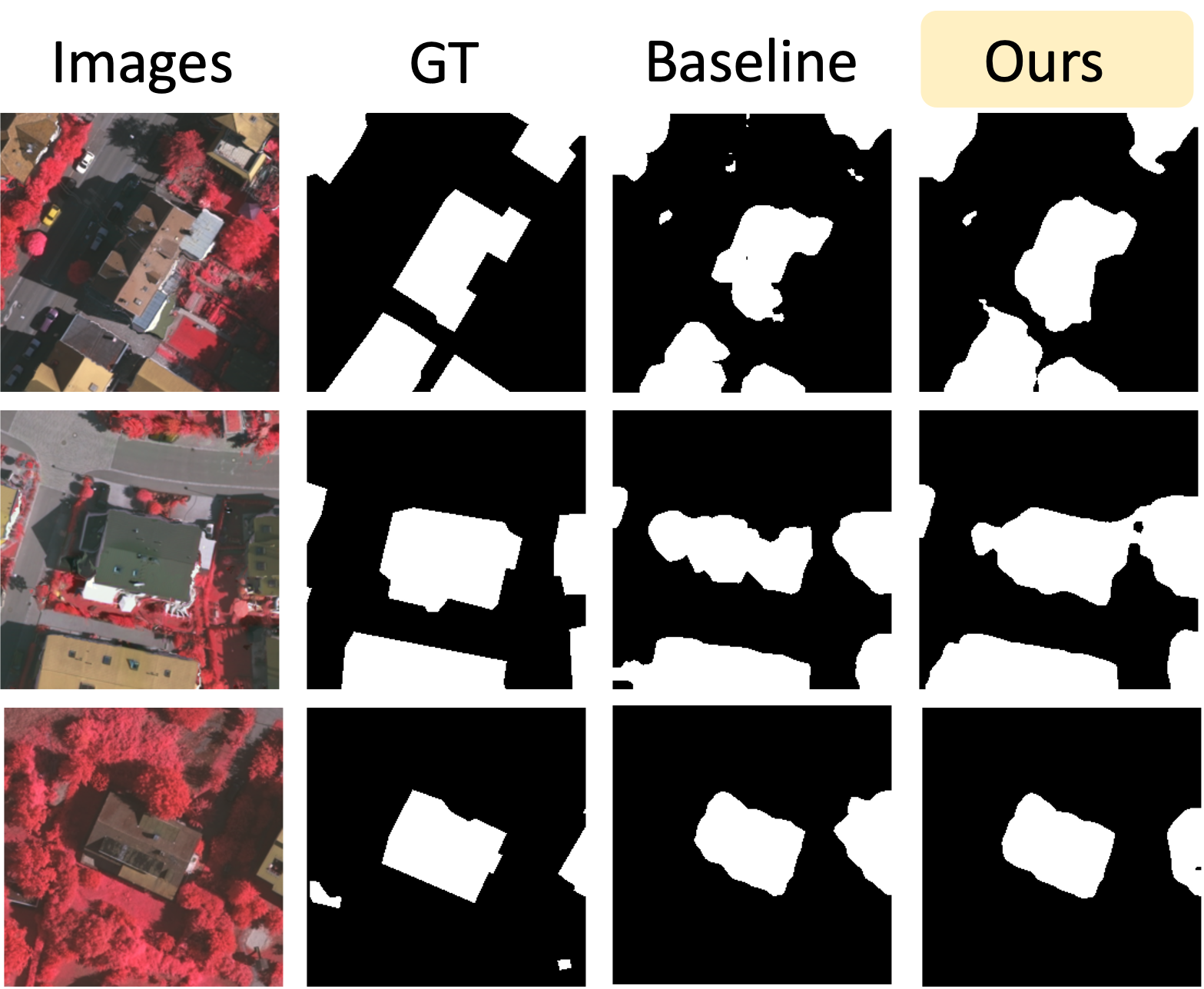
Figure 2: Qualitative results on Vaihingen dataset. Our model performs well despite the small sample size.

Results and Discussion. We use the average Intersection over Union (IoU) to evaluate the performance on Vaihingen dataset: the baseline yields 68.9 while our model without TMDlayer achieves 73.5 and our complete model with TMDlayer achieves 74.6, which is a significant improvement in terms of IoU. This experiment shows that our TMDlayer can be built on top of another dynamical system and can provide additional benefits. Qualitative results of the baseline and our model are shown in Fig. 2. Our method tends to predict a more precise shape/boundary, and also fixes some flaws/errors relative to the baseline results.

4.4 Few-shot learning

In $N$-way $B$-shot few-shot learning, the input is a set of $N\times B$ samples which naturally forms a fully connected graph. This serves to construct the differential operator $L_{m}$. To provide context for where and how our TMDlayer will be instantiated, we note that [25] proposed a GNN approach (EGNN) for few-shot learning and this model achieves state-of-the-art performance. We show that by adding our TMDlayer, the performance increases by a clear margin.

4.4.1 Problem formulation

Few-shot learning classification seeks to learn a classifier given only a few training samples for every class. Each few-shot classification task $\mathcal{T}$ contains a support set $S$ which is a set of labeled input-label pairs and a query set $Q$ (an unlabeled set where the learned classifier is evaluated). Given $B$ labeled samples for each of $N$ classes in the support set $S$, the problem is a $N$-way $B$-shot classification problem.

4.4.2 Role of TMDlayer: Use in graph neural network

Let $\mathcal{G}$ be the graph formed by samples from the task $\mathcal{T}$, with nodes denoted as $\mathcal{V}:=\{V_{i}\}_{i=1,...,|\mathcal{T}|}$. The node feature update equation is designed as (we refer readers to [25] or our appendix for more details about the network)

$$v_{i}^{l}=\text{NodeUpdate}(\{v_{i}^{l-1}\},\{e_{ij}^{l-1}\};\theta_{v}^{l}),$$ (14)

where $v_{i}^{l}$ is the feature of node $i$ at $l$-th layer, $e_{ij}$ is the edge feature between node $i$ and node $j$, and $\theta$ refers to the parameters in the update function. We abstract (14) as $v_{i}^{l}=f(v_{i}^{l-1})$ and use our TMDlayer as,

$$v_{i}^{l}=f(v_{i}^{l-1})+\Delta t\cdot L_{m}f(v_{i}^{l-1}).$$ (15)

Remark 3

In (15), the $L_{m}$ is constructed using samples from the same episode, and $f$ is a GNN module updating the node features using all node features and edge features.

4.4.3 Experimental results

Dataset. We follow [25] to conduct experiments on miniImageNet, proposed by [51] and derived from ILSVRC-12 dataset [46]. Images are sampled from $100$ different classes with $600$ samples per class (size $84\times 84$ pixels). We use the same splits as in [43, 25]: $64$, $16$ and $20$ classes for training, validation and testing respectively.

Network architecture and training details. We use the same graph neural network architecture and follow the training strategy as in [25] by utilizing the code provided by the authors. We add our TMDlayer as shown in (15) to each node update layer in the graph neural network, with a latent dimension of $16$ for constructing $L_{m}$. We follow [25] to conduct experiments for 5-way 5-shot learning, in both transductive and non-transductive settings, as well as for both supervised and semi-supervised settings. The network is trained with Adam optimizer with an initial learning rate of $5\times 10^{-4}$ and weight decay of $10^{-6}$. The learning rate is cut in half every $15000$ episodes. For evaluation, each test episode was formed by randomly sampling $15$ queries for each of $5$ classes, and the performance is averaged over $600$ randomly generated episodes from the test set. Note that the feature embedding module is a convolutional neural network which consists of four blocks (following [25]) and used in most few-shot learning models without any skip connections. Thus, Resnet-based models are excluded from the table for a fair comparison. We refer the reader to [25] or the appendix for more training and evaluation details.

Results. The performance of supervised and semi-supervised 5-way 5-shot learning is given in Tables 4–5 respectively. Our TMDlayer leads to consistent and clear improvements in both supervised and semi-supervised settings (also for transductive/non-transductive settings).

Model	Trans.	Accuracy(%)
Matching Networks [51]	No	55.30
Reptile [40]	No	62.74
Prototypical Net [47]	No	65.77
GNN [18]	No	66.41
EGNN [25]	No	66.85
Ours	No	68.35
MAML [17]	BN	63.11
Reptile + BN [40]	BN	65.99
Relation Net [50]	BN	67.07
MAML + Transduction [17]	Yes	66.19
TNP [35]	Yes	69.43
TPN (Higher K) [35]	Yes	69.86
EGNN+Transduction [25]	Yes	76.37
Ours+Transduction	Yes	77.78

Table 4: Results of 5-way 5-shot learning on miniImageNet, averaged over 600 test episodes. “Ours” means EGNN plus our TMDlayer.“BN” means that the query batch statistics are used instead of global batch normalization parameters.

	Labeled Ratio (5-way 5-shot)
Training method	20%	40%	60%	1000%
GNN-semi [18]	52.45	58.76	-	66.41
EGNN-semi [25]	61.88	62.52	63.53	66.85
Ours	63.14	64.32	64.83	68.35
EGNN-semi(T) [25]	63.62	64.32	66.37	76.37
Ours(T)	64.84	66.43	68.62	77.78

Table 5: Accuracy of semi-supervised few-shot classification. “Ours” means EGNN plus our TMDlayer.

4.5 Runtime overhead/Relation with augmentation

Runtime overhead. Our construction does involve some training time overhead because of computing the kernel matrix, and varies depending on the use case. For reference, the overhead is $10\%$ in §4.2, $11\%$ in §4.3 and $1\%$ in §4.4.

Relationship with data augmentation. Data augmentation and TMDLayer are complementary, not mutually exclusive. In all our experiments, the baselines use data augmentations (e.g., random rotation or cropping). Our TMDLayer offers benefits, above and beyond augmentation.

5 Discussion and Conclusions

We proposed an SDE based framework that allows a unified view of several different learning tasks in vision. Our framework is beneficial where data generation (or the data itself) can be described using stochastic processes, or more specifically diffusion operators. This is particularly useful in settings where obtaining a deterministic model of the image manifold or learning density functions are impossible or challenging due to high sample complexity requirements. Our TMDlayer does not require explicit generation of diffused samples, especially during training, making it computationally efficient. The “process” of which the provided data sample is a snapshot and whose characterization is enabled by our TMDlayer, also appears to have implications for robust learning. Indeed, if the parameters that define the process are explicitly optimized, we should be able to establish an analogy between the resultant model as a stochastic/simpler version of recent results for certified margin radius maximization [60] which often require access to Monte Carlo sampling oracles [11]. We believe that periodicity in SDEs for data augmentation is an important missing ingredient – for instance – this may help model seasonal patterns in disease progression studies for predictions, automatically. For this purpose, tools from Floquet theory may allow us to consider transformed versions of the process, potentially with simplified generators. Our code is available at https://github.com/zihangm/neural-tmd-layer .

References

- [1] Matan Atzmon, Haggai Maron, and Yaron Lipman. Point convolutional neural networks by extension operators. arXiv preprint arXiv:1803.10091, 2018.
- [2] Ralf Banisch, Zofia Trstanova, Andreas Bittracher, Stefan Klus, and Péter Koltai. Diffusion maps tailored to arbitrary non-degenerate itô processes. Applied and Computational Harmonic Analysis, 48(1):242–265, 2020.
- [3] Mikhail Belkin and Partha Niyogi. Laplacian eigenmaps for dimensionality reduction and data representation. Neural computation, 15(6):1373–1396, 2003.
- [4] Mikhail Belkin, Partha Niyogi, and Vikas Sindhwani. Manifold regularization: A geometric framework for learning from labeled and unlabeled examples. Journal of machine learning research, 7(11), 2006.
- [5] Iz Beltagy, Matthew E Peters, and Arman Cohan. Longformer: The long-document transformer. arXiv preprint arXiv:2004.05150, 2020.
- [6] Vicent Caselles, Ron Kimmel, and Guillermo Sapiro. Geodesic active contours. International journal of computer vision, 22(1):61–79, 1997.
- [7] Tony F Chan and Luminita A Vese. Active contours without edges. IEEE Transactions on image processing, 10(2):266–277, 2001.
- [8] Pratik Chaudhari and Stefano Soatto. Stochastic gradient descent performs variational inference, converges to limit cycles for deep networks. In 2018 Information Theory and Applications Workshop (ITA), pages 1–10. IEEE, 2018.
- [9] Liang-Chieh Chen, George Papandreou, Iasonas Kokkinos, Kevin Murphy, and Alan L Yuille. Deeplab: Semantic image segmentation with deep convolutional nets, atrous convolution, and fully connected crfs. IEEE transactions on pattern analysis and machine intelligence, 40(4):834–848, 2017.
- [10] Ricky TQ Chen, Yulia Rubanova, Jesse Bettencourt, and David Duvenaud. Neural ordinary differential equations. arXiv preprint arXiv:1806.07366, 2018.
- [11] Jeremy Cohen, Elan Rosenfeld, and Zico Kolter. Certified adversarial robustness via randomized smoothing. In International Conference on Machine Learning, pages 1310–1320. PMLR, 2019.
- [12] Taco S Cohen, Mario Geiger, Jonas Köhler, and Max Welling. Spherical cnns. arXiv preprint arXiv:1801.10130, 2018.
- [13] Ronald R Coifman and Stéphane Lafon. Diffusion maps. Applied and computational harmonic analysis, 21(1):5–30, 2006.
- [14] Ekin D Cubuk, Barret Zoph, Dandelion Mane, Vijay Vasudevan, and Quoc V Le. Autoaugment: Learning augmentation strategies from data. In Proceedings of the IEEE/CVF Conference on Computer Vision and Pattern Recognition, pages 113–123, 2019.
- [15] Emilien Dupont, Arnaud Doucet, and Yee Whye Teh. Augmented neural odes. arXiv preprint arXiv:1904.01681, 2019.
- [16] Carlos Esteves, Christine Allen-Blanchette, Ameesh Makadia, and Kostas Daniilidis. Learning so(3) equivariant representations with spherical cnns. CoRR, 2017.
- [17] Chelsea Finn, Pieter Abbeel, and Sergey Levine. Model-agnostic meta-learning for fast adaptation of deep networks. In International Conference on Machine Learning, pages 1126–1135. PMLR, 2017.
- [18] Victor Garcia and Joan Bruna. Few-shot learning with graph neural networks. arXiv preprint arXiv:1711.04043, 2017.
- [19] Meng-Hao Guo, Jun-Xiong Cai, Zheng-Ning Liu, Tai-Jiang Mu, Ralph R Martin, and Shi-Min Hu. Pct: Point cloud transformer. arXiv preprint arXiv:2012.09688, 2020.
- [20] Moritz Hardt, Ben Recht, and Yoram Singer. Train faster, generalize better: Stability of stochastic gradient descent. In International Conference on Machine Learning, pages 1225–1234. PMLR, 2016.
- [21] Bharath Hariharan, Pablo Arbeláez, Ross Girshick, and Jitendra Malik. Hypercolumns for object segmentation and fine-grained localization. In Proceedings of the IEEE conference on computer vision and pattern recognition, pages 447–456, 2015.
- [22] Ali Hatamizadeh, Debleena Sengupta, and Demetri Terzopoulos. End-to-end deep convolutional active contours for image segmentation. arXiv preprint arXiv:1909.13359, 2019.
- [23] Kaiming He, Xiangyu Zhang, Shaoqing Ren, and Jian Sun. Deep residual learning for image recognition. In Proceedings of the IEEE conference on computer vision and pattern recognition, pages 770–778, 2016.
- [24] Ehsan Kharazmi, Zhongqiang Zhang, and George Em Karniadakis. Variational physics-informed neural networks for solving partial differential equations. arXiv preprint arXiv:1912.00873, 2019.
- [25] Jongmin Kim, Taesup Kim, Sungwoong Kim, and Chang D Yoo. Edge-labeling graph neural network for few-shot learning. In Proceedings of the IEEE/CVF Conference on Computer Vision and Pattern Recognition, pages 11–20, 2019.
- [26] Roman Klokov and Victor Lempitsky. Escape from cells: Deep kd-networks for the recognition of 3d point cloud models. In Proceedings of the IEEE International Conference on Computer Vision, pages 863–872, 2017.
- [27] Artem Komarichev, Zichun Zhong, and Jing Hua. A-cnn: Annularly convolutional neural networks on point clouds. In Proceedings of the IEEE/CVF Conference on Computer Vision and Pattern Recognition, pages 7421–7430, 2019.
- [28] Alex Krizhevsky, Geoffrey Hinton, et al. Learning multiple layers of features from tiny images. 2009.
- [29] Hiroshi Kunita. Stochastic flows and stochastic differential equations, volume 24. Cambridge university press, 1997.
- [30] Truc Le and Ye Duan. Pointgrid: A deep network for 3d shape understanding. In Proceedings of the IEEE conference on computer vision and pattern recognition, pages 9204–9214, 2018.
- [31] Jiaxin Li, Ben M Chen, and Gim Hee Lee. So-net: Self-organizing network for point cloud analysis. In Proceedings of the IEEE conference on computer vision and pattern recognition, pages 9397–9406, 2018.
- [32] Zongyi Li, Nikola Kovachki, Kamyar Azizzadenesheli, Burigede Liu, Kaushik Bhattacharya, Andrew Stuart, and Anima Anandkumar. Fourier neural operator for parametric partial differential equations. arXiv preprint arXiv:2010.08895, 2020.
- [33] Huan Ling, Jun Gao, Amlan Kar, Wenzheng Chen, and Sanja Fidler. Fast interactive object annotation with curve-gcn. In Proceedings of the IEEE/CVF Conference on Computer Vision and Pattern Recognition, pages 5257–5266, 2019.
- [34] Xuanqing Liu, Si Si, Qin Cao, Sanjiv Kumar, and Cho-Jui Hsieh. Neural sde: Stabilizing neural ode networks with stochastic noise. arXiv preprint arXiv:1906.02355, 2019.
- [35] Y Liu, J Lee, M Park, S Kim, E Yang, SJ Hwang, and Y Yang. Learning to propagate labels: Transductive propagation network for few-shot learning. In 7th International Conference on Learning Representations, ICLR 2019, 2019.
- [36] Ravi Malladi, James A Sethian, and Baba C Vemuri. Shape modeling with front propagation: A level set approach. IEEE transactions on pattern analysis and machine intelligence, 17(2):158–175, 1995.
- [37] Diego Marcos, Devis Tuia, Benjamin Kellenberger, Lisa Zhang, Min Bai, Renjie Liao, and Raquel Urtasun. Learning deep structured active contours end-to-end. In Proceedings of the IEEE Conference on Computer Vision and Pattern Recognition, pages 8877–8885, 2018.
- [38] Luke Melas-Kyriazi. The Geometry of Semi-Supervised Learning. PhD thesis, Harvard University Cambridge, Massachusetts, 2020.
- [39] Craig Michoski, Miloš Milosavljević, Todd Oliver, and David R Hatch. Solving differential equations using deep neural networks. Neurocomputing, 399:193–212, 2020.
- [40] Alex Nichol, Joshua Achiam, and John Schulman. On first-order meta-learning algorithms. arXiv preprint arXiv:1803.02999, 2018.
- [41] Charles R Qi, Hao Su, Kaichun Mo, and Leonidas J Guibas. Pointnet: Deep learning on point sets for 3d classification and segmentation. In Proceedings of the IEEE conference on computer vision and pattern recognition, pages 652–660, 2017.
- [42] Guo-Jun Qi, Liheng Zhang, Feng Lin, and Xiao Wang. Learning generalized transformation equivariant representations via autoencoding transformations. IEEE Transactions on Pattern Analysis and Machine Intelligence, 2020.
- [43] Sachin Ravi and Hugo Larochelle. Optimization as a model for few-shot learning. ICLR 2017, 2017.
- [44] Remi Ronfard. Region-based strategies for active contour models. International journal of computer vision, 13(2):229–251, 1994.
- [45] Leonid I Rudin and Stanley Osher. Total variation based image restoration with free local constraints. In Proceedings of 1st International Conference on Image Processing, volume 1, pages 31–35. IEEE, 1994.
- [46] Olga Russakovsky, Jia Deng, Hao Su, Jonathan Krause, Sanjeev Satheesh, Sean Ma, Zhiheng Huang, Andrej Karpathy, Aditya Khosla, Michael Bernstein, et al. Imagenet large scale visual recognition challenge. International journal of computer vision, 115(3):211–252, 2015.
- [47] Jake Snell, Kevin Swersky, and Richard S Zemel. Prototypical networks for few-shot learning. arXiv preprint arXiv:1703.05175, 2017.
- [48] Riccardo Spezialetti, Samuele Salti, and Luigi Di Stefano. Learning an effective equivariant 3d descriptor without supervision. In Proceedings of the IEEE/CVF International Conference on Computer Vision, pages 6401–6410, 2019.
- [49] Özlem N Subakan and Baba C Vemuri. A quaternion framework for color image smoothing and segmentation. International Journal of Computer Vision, 91(3):233–250, 2011.
- [50] Flood Sung, Yongxin Yang, Li Zhang, Tao Xiang, Philip HS Torr, and Timothy M Hospedales. Learning to compare: Relation network for few-shot learning. In Proceedings of the IEEE conference on computer vision and pattern recognition, pages 1199–1208, 2018.
- [51] Oriol Vinyals, Charles Blundell, Timothy Lillicrap, Koray Kavukcuoglu, and Daan Wierstra. Matching networks for one shot learning. arXiv preprint arXiv:1606.04080, 2016.
- [52] Yue Wang, Yongbin Sun, Ziwei Liu, Sanjay E Sarma, Michael M Bronstein, and Justin M Solomon. Dynamic graph cnn for learning on point clouds. Acm Transactions On Graphics (tog), 38(5):1–12, 2019.
- [53] Wenxuan Wu, Zhongang Qi, and Li Fuxin. Pointconv: Deep convolutional networks on 3d point clouds. In Proceedings of the IEEE/CVF Conference on Computer Vision and Pattern Recognition, pages 9621–9630, 2019.
- [54] Zhirong Wu, Shuran Song, Aditya Khosla, Fisher Yu, Linguang Zhang, Xiaoou Tang, and Jianxiong Xiao. 3d shapenets: A deep representation for volumetric shapes. In Proceedings of the IEEE conference on computer vision and pattern recognition, pages 1912–1920, 2015.
- [55] Saining Xie, Sainan Liu, Zeyu Chen, and Zhuowen Tu. Attentional shapecontextnet for point cloud recognition. In Proceedings of the IEEE Conference on Computer Vision and Pattern Recognition, pages 4606–4615, 2018.
- [56] Yunyang Xiong, Zhanpeng Zeng, Rudrasis Chakraborty, Mingxing Tan, Glenn Fung, Yin Li, and Vikas Singh. Nyströmformer: A nyström-based algorithm for approximating self-attention. arXiv preprint arXiv:2102.03902, 2021.
- [57] Chenyang Xu, Dzung L Pham, and Jerry L Prince. Image segmentation using deformable models. Handbook of medical imaging, 2(20):0, 2000.
- [58] Jialin Yuan, Chao Chen, and Li Fuxin. Deep variational instance segmentation. NeurIPS 2020, 2020.
- [59] Zhanpeng Zeng, Yunyang Xiong, Sathya Ravi, Shailesh Acharya, Glenn M Fung, and Vikas Singh. You only sample (almost) once: Linear cost self-attention via bernoulli sampling. In International Conference on Machine Learning, pages 12321–12332. PMLR, 2021.
- [60] Xingjian Zhen, Rudrasis Chakraborty, and Vikas Singh. Simpler certified radius maximization by propagating covariances. In Proceedings of the IEEE/CVF Conference on Computer Vision and Pattern Recognition, pages 7292–7301, 2021.
- [61] Jun-Yan Zhu, Philipp Krähenbühl, Eli Shechtman, and Alexei A Efros. Generative visual manipulation on the natural image manifold. In European conference on computer vision, pages 597–613. Springer, 2016.