Footprints of the Kitaev spin liquid in the Fano lineshape of the Raman active optical phonons

Abstract

We develop a theoretical description of the Raman spectroscopy in the spin-phonon coupled Kitaev system and show that it can provide observable signatures of fractionalized excitations characteristic of the underlying spin liquid phase. In particular, we obtain the explicit form of the phonon modes and construct the coupling Hamiltonian based on the $D_{3d}$ symmetry. We then systematically compute the Raman intensity and show that the spin-phonon coupling renormalizes phonon propagators and generates the salient Fano linshape. We find that the temperature evolution of the Fano lineshape displays two crossovers, and the low temperature crossover shows pronounced magnetic field dependence. We thus identify the observable effect of the Majorana fermions and the $Z_{2}$ gauge fluxes encoded in the Fano lineshape. Our results are consistent with the phonon Raman scattering experiments in the candidate material $\alpha\textmd{-RuCl}_{3}$.

Introduction.– Raman spectroscopy has proven to be a sensitive experimental probe to study the ground state properties and the dynamics of various strongly correlated systems Devereaux and Hackl (2007). For magnetic insulators, Raman process couples to the dynamically induced electron-hole pair, that connects to the low-energy magnetic states. In magnetically ordered states, the magnetic Raman response shows polarization-dependent peak structure, arising predominantly from one- and two-magnon excitations Fleury and Loudon (1968); Shastry and Shraiman (1990); Chubukov and Frenkel (1995); Perkins and Brenig (2008); Perkins et al. (2013); Yang et al. (2021). In quantum spin liquid (QSL) phase, the Raman spectrum of such low-energy states reveals characteristic low-energy continua, which are fundamentally different from the dispersive collective modes in ordered states. These continua reflect the fractionalization of spins, a hallmark of QSL Ko et al. (2010); Knolle et al. (2014a); Perreault et al. (2015, 2016a, 2016b); Nasu et al. (2016); Rousochatzakis et al. (2019); Fu et al. (2017); Metavitsiadis et al. (2021).

Recently, significant efforts have been made in the investigation of quantum spin-liquid (QSL) state of matter. Mott insulators with strong spin-orbit coupling, e.g $\alpha$-$\textmd{RuCl}_{3}$ Plumb et al. (2014); Sears et al. (2015); Banerjee et al. (2016, 2017, 2018); Little et al. (2017); Sandilands et al. (2015); Li et al. (2019); Wulferding et al. (2020); Sahasrabudhe et al. (2020); Lin et al. (2020); Wang et al. (2020), are promising to realize Kitaev QSL. This QSL is motivated by the famous Kitaev spin model with bond-dependent Ising interactions on a two-dimensional honeycomb lattice Kitaev (2006). It is exactly solvable with known gapless QSL ground state. In this model, the spins fractionalize into static $Z_{2}$ gauge fluxes and itinerant Majorana fermions amenable to experimental detection.

While various dynamical probes Knolle et al. (2014a, b, 2015); Halász et al. (2016, 2019); Rousochatzakis et al. (2019); Wan and Armitage (2019) have been exploited in several materials to look for signatures of spin fractionalization and their proximity to the Kitaev QSL, employing phonon dynamics and the spin-lattice coupling to detect Kitaev QSL is less investigated. It was recently suggested that sound attenuation from the phonon decaying into a pair of Majorana fermions Metavitsiadis and Brenig (2020); Ye et al. (2020); Feng et al. (2021) and the Hall viscosity induced by time-reversal breaking spin Hamiltonian Ye et al. (2020); Feng et al. (2021) may potentially serve as such probe. The importance of the spin-phonon coupling in the Kitaev materials is also shown in the interpretation of the thermal Hall transport measurements  Kasahara et al. (2018); Ye et al. (2018); Vinkler-Aviv and Rosch (2018).

In this letter, we focus on the Raman spectroscopy of optical phonons, and particularly the salient Fano line shape, which arises when the phonon resonance peak couples to the magnetic continuum Fano (1961). This effect is attributed to spin-dependent electron polarizability Suzuki and Kamimura (1973); Moriya (1967), which involves a microscopic description of both spin-photon coupling and spin-phonon couplings. A recent work Ref. Metavitsiadis et al. (2021) shows that even the simplest form of the couplings can give rise to the Fano line shape. In the experimental studies of the candidate material $\alpha$-$\textmd{RuCl}_{3}$ Sandilands et al. (2015); Glamazda et al. (2017); Li et al. (2019); Wulferding et al. (2020); Sahasrabudhe et al. (2020); Lin et al. (2020), the pronounced temperature and field dependence of Fano lineshape indicate rich information about the underlying spin liquid phase that awaits exploration. However, up to now a clear theoretical description of the Raman scattering in a Kitaev spin-phonon coupled system is still missing, mainly due to the lack of proper description of spin-phonon and spin-photon couplings Metavitsiadis et al. (2021).

Here, we make use of the $D_{3d}$ group symmetry of the Kitaev model You et al. (2012) and propose a theory to describe the Raman scattering of the Kitaev spin-phonon coupled system. We show that our theory, in which the spin-phonon coupling and spin-photon coupling are explicitly built from the symmetry constraints, quantitatively characterizes the temperature evolution and field dependence of the Fano lineshape of two low-energy optical phonons, observed in the Raman scattering experiments in $\alpha$-$\textmd{RuCl}_{3}$ Sandilands et al. (2015); Glamazda et al. (2017); Li et al. (2019); Wulferding et al. (2020); Sahasrabudhe et al. (2020); Lin et al. (2020). These results reveal clear effects of the Majorana fermions and the $Z_{2}$ fluxes, which provide observable signatures for experimental detection of Kitaev QSL.

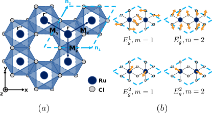
Figure 1: (a) Crystal structure of $\alpha$-RuCl₃. The unit cell shown in blue dashed lines is defined by $\mathbf{n_{1}}=(\sqrt{3},0)$ and $\mathbf{n_{2}}=\big{(}\frac{3}{2},\frac{\sqrt{3}}{2}\big{)}$ and includes two Ru³⁺ and six Cl^- ions. $\mathbf{M_{x,y}}=\big{(}\pm\frac{\sqrt{3}}{2},\frac{1}{2}\big{)}$ and $\mathbf{M_{z}}=(0,-1)$ are nearest neighbor vectors. The sites $\mathbf{r},\mathbf{r^{\prime}},\mathbf{r^{\prime\prime}}$ form a generic three-spin link $\braket{\mathbf{r},\mathbf{r^{\prime}},\mathbf{r^{\prime\prime}}}_{yx}$ as described in the text. (b) Visualization of the eigenmodes of $E^{1}_{g}$ and $E^{2}_{g}$ phonons in $xy$ plane, obtained by linear representation theory (see Sec. A of SM).

Model.– We consider the spin-phonon Hamiltonian

$$H=H_{\text{s}}+H_{\mathrm{ph}}+H_{\textmd{s-ph}}.$$ (1)

The first term is the extended Kitaev honeycomb model Kitaev (2006), $H_{\text{s}}=$ $-J\sum_{\alpha,{\bf r}\in A}\sigma_{\bf r}^{\alpha}\sigma_{{\bf r}+{\bf M}_{\alpha}}^{\alpha}-\kappa\sum_{\langle{\bf r},{\bf r}^{\prime},{\bf r}^{\prime\prime}\rangle_{\alpha\gamma}}$ $\sigma^{\alpha}_{{\bf r}}\sigma^{\beta}_{{\bf r}^{\prime}}\sigma^{\gamma}_{{\bf r}^{\prime\prime}}$, where $\sigma^{\alpha}_{\bf r}$ are the Pauli matrices, $\alpha=x,y,z$ and ${\bf M}_{\alpha}$ are nearest neighbor vectors; $J$ denotes the Kitaev interaction; $\kappa$ is the strength of the time reversal symmetry breaking term, which mimics the effect of an external magnetic field . The three-spin link notation $\langle{\bf r},{\bf r}^{\prime},{\bf r}^{\prime\prime}\rangle_{\alpha\gamma}$ labels bonds ${\bf r}{\bf r}^{\prime}$, ${\bf r}^{\prime}{\bf r}^{\prime\prime}$ by type $\alpha,\gamma$ respectively and $\beta\neq\alpha,\gamma$. ${\bf r},{\bf r}^{\prime},{\bf r}^{\prime\prime}$ are counter-clockwise ordered adjacent sites (see Fig. 1 (a)). The leading order term in this Hamiltonian, i.e., the pure Kitaev model, has a symmetry described by $D_{3d}$ group . The $\kappa$ term lowers the symmetry to the $S_{6}$ group by breaking the two-fold rotation, but we still consider $D_{3d}$ symmetry which gives the strongest constraint on the theory.

$H_{s}$ is exactly solvable by the four Majorana fermion representation of spin Kitaev (2006), $\sigma_{\bf r}^{\alpha}=ib_{\bf r}^{\alpha}c_{\bf r}$. In this representation, $H_{\text{s}}=$ $\frac{1}{4}\sum_{\langle{\bf r}{\bf r}^{\prime}\rangle}h_{{\bf r}{\bf r}^{\prime}}c_{\bf r}c_{{\bf r}^{\prime}}$, where $h_{{\bf r}{\bf r}^{\prime}}=$ $2J\,i\eta_{{\bf r}{\bf r}^{\prime}}+2\kappa\,i\eta_{{\bf r}{\bf r}^{\prime}}\eta_{{\bf r}^{\prime}{\bf r}^{\prime\prime}}$ is the Hamiltonian matrix and $\eta_{{\bf r}{\bf r}^{\prime}}=ib_{\bf r}^{\alpha}b_{{\bf r}^{\prime}}^{\alpha}=\pm 1$ is the static $Z_{2}$ gauge field on the $\alpha$-bond, which generates conserved $Z_{2}$ fluxes. Within each flux sector, $H_{\textmd{s}}$ can be further diagonalized to be $H_{\textmd{s}}=$ $\sum_{i}\epsilon_{i}\left(\beta^{\dagger}_{i}\beta_{i}-1/2\right)$, where $\epsilon_{i}$ are the fermionic energy levels and $\beta_{i}^{\dagger},\beta_{i}$ correspond to the fermionic eigenmodes. Hereafter, the energy and temperature unit will be $J$ unless otherwise specified, which is estimated to be $J\approx 2$ meV = 23 K Sandilands et al. (2015) .

The second term in Eq.(1) is the free phonon Hamiltonian $H_{\mathrm{ph}}=$ $H_{\mathrm{ph}}\left(p_{i}(\mathbf{r}),q_{i}(\mathbf{r})\right)$, where $q_{i}(\mathbf{r})=(x_{1},y_{1},z_{1},\ldots,x_{8},y_{8},z_{8})_{\bf r}$ denotes the displacement field in a unit cell at ${\bf r}$, which contains two Ru³⁺ and six Cl^- ions, shown in Fig. 1(a) and Fig. S1 in the Supplementary Material (SM) Sup ; $p_{i}(\mathbf{r})$ is the corresponding momentum. Hereafter, we will drop the ${\bf r}$ dependence in phonon fields, since the long wavelength of incident light leads to uniform lattice vibrations. By using the $D_{3d}$ symmetry of $\alpha$-RuCl₃, i.e. $[D_{3d},H_{\textmd{ph}}]=0$, the eigenmodes of $H_{\textmd{ph}}$ are solved to be the irreducible representations (irreps) of the group, written as linear superpositions of the displacement field: $u_{\Gamma m}=\sum_{i=1}^{24}u_{\Gamma m,i}q_{i}$. Here, $\Gamma$ labels the irrep, i.e. $\Gamma=2A_{1g}+2A_{2g}+4E_{g}+A_{1u}+3A_{2u}+4E_{u}$, among which the Raman active modes are $\Gamma_{R}=2A_{1g}+4E_{g}$ Guizzetti et al. (1979); Li et al. (2019), and $m$ is the dimension of the irrep. [See Sec. A in the SM for detailed analysis Sup ]. In this work, we focus on the two low-energy phonon modes in the Raman spectroscopy Lin et al. (2020); Li et al. (2019); Sandilands et al. (2015): $E_{\textmd{g}}^{1}$ and $E_{\textmd{g}}^{2}$, whose energies ($\sim$ 14 meV and 20 meV respectively) are comparable to the magnetic continuum’s energy. They are visualized in Fig.1(b). The corresponding free phonon Matsubara propagators are written as $\mathcal{D}^{(0)}_{\Gamma m,\Gamma^{\prime}m^{\prime}}(i\omega_{n})=-\langle T_{\tau}u_{\Gamma m}(\tau)u_{\Gamma^{\prime}m^{\prime}}(0)\rangle_{\omega_{n}}=\frac{2\omega_{\Gamma}}{\left(i\omega_{n}\right)^{2}-\omega_{\Gamma}^{2}}\delta_{\Gamma\Gamma^{\prime}}\delta_{mm^{\prime}}$, where $\omega_{\Gamma}$ is the frequency of the optical phonon, and $T_{\tau}$ is the imaginary time ordering operator.

The third term in Eq.(1) is the spin-phonon coupling Hamiltonian. It originates from the change of the Kitaev interaction in response to the lattice vibration: $J(q_{i})=J+\sum_{\Gamma,m}\frac{\mathrm{d}J(q_{i})}{\mathrm{d}u_{\Gamma m}}u_{\Gamma m}+\cdots$, where $\frac{\mathrm{d}J(q_{i})}{\mathrm{d}u_{\Gamma m}}$ is the gradient along $u_{\Gamma m}$ direction in the manifold of the displacement field. The $D_{3d}$ invariant spin-phonon Hamiltonian is built as

$$H_{\textmd{s-ph}}=\sum_{\Gamma,m}\lambda_{\Gamma}\Sigma_{\Gamma m}u_{\Gamma m},$$ (2)

where $\Sigma_{E_{g},1}=$ $\sum_{\mathbf{r}}(\sigma_{\mathbf{r}}^{x}\sigma_{\mathbf{r}+\mathbf{M}_{x}}^{x}+$ $\sigma_{\mathbf{r}}^{y}\sigma_{\mathbf{r}+\mathbf{M}_{y}}^{y}-$ $2\sigma_{\mathbf{r}}^{z}\sigma_{\mathbf{r}+\mathbf{M}_{z}}^{z})$ and $\Sigma_{E_{g},2}=$ $\sum_{\mathbf{r}}(-\sqrt{3}\sigma_{\mathbf{r}}^{x}\sigma_{\mathbf{r}+\mathbf{M}_{x}}^{x}+$ $\sqrt{3}\sigma_{\mathbf{r}}^{y}\sigma_{\mathbf{r}+\mathbf{M}_{y}}^{y})$ are irreducible representations (irreps) of $D_{3d}$, and $\lambda_{\Gamma}$ are the coupling constants.

As shown by the perturbative calculation in the SM, the phonon propagator is renormalized by the spin-phonon coupling. According to the Dyson’s equation, ${\hat{\mathcal{D}}}=$ $\left[{({\hat{\mathcal{D}}}^{(0)}})^{-1}-{\hat{\Pi}}\right]^{-1}$, where ${\hat{\Pi}}$ is the polarization bubble defined as

$$\Pi_{\Gamma m,\Gamma^{\prime}m^{\prime}} =-\lambda_{\Gamma}\lambda_{\Gamma^{\prime}}\left\langle T_{\tau}\Sigma_{\Gamma m}(\tau)\Sigma_{\Gamma^{\prime}m^{\prime}}(0)\right\rangle.$$ (3)

$\mathcal{D}_{\Gamma m,\Gamma^{\prime}m^{\prime}}$ and $\Pi_{\Gamma m,\Gamma^{\prime}m^{\prime}}$ are 4 by 4 matrices, in which the 2 by 2 off-diagonal blocks correspond to the mixing between $E_{g}^{1}$ and $E_{g}^{2}$ phonon modes. The components of the off-diagonal blocks are negligible, since the corresponding phonon peaks in the Raman spectroscopy are well separated Li et al. (2019).

As will be seen later, the phonon Raman peak parameters, such as the width, center position and asymmetry factor, are directly related to the real and imaginary parts of the fermionic loop diagrams contained in $\hat{\Pi}$ whose temperature dependence at various values of $\kappa$ is shown in Fig. S1 of SM. When temperature increases, both $\operatorname{Re}\hat{\Pi}$ and $\operatorname{Im}\hat{\Pi}$, evaluated at the bare phonon energies, generically display two-stage decrease which is characterized by two crossover temperatures. We can thus expect that this stage-wise temperature dependence in $\hat{\Pi}$ should be reflected in the temperature dependence of the phonon peak parameters, as shown next.

Raman response.– The Raman scattering of the spin-phonon coupled Kitaev system (1) is described by the Raman operator: ${\mathcal{R}}$=$\sum_{\mu\mu^{\prime}}\left({\mathcal{R}}^{\mu\mu^{\prime}}_{\textmd{em-ph}}+{\mathcal{R}}^{\mu\mu^{\prime}}_{\textmd{em-s}}\right)E^{\mu}_{\textmd{in}}E^{\mu^{\prime}}_{\textmd{out}}$, where $E^{\mu}_{\textmd{in}}$, $E^{\mu^{\prime}}_{\textmd{out}}$ are the electromagnetic fields of the incoming and outgoing light. The second rank symmetric tensors ${\mathcal{R}}^{\mu\mu^{\prime}}_{\textmd{em-ph}}$ and ${\mathcal{R}}^{\mu\mu^{\prime}}_{\textmd{em-s}}$ microscopically describe the polarizability change of the electronic medium in response to the excitations of phonons and spins Dresselhaus et al. (2007). Under the $D_{3d}$ symmetry constraint on the Raman operator, ${\mathcal{R}}^{\mu\mu^{\prime}}_{\textmd{em-ph}}$ is given by

$${\mathcal{R}}^{\mu\mu^{\prime}}_{\textmd{em-ph}}=\sum_{\Gamma,m}\mu_{\Gamma}R_{\Gamma m}^{\mu\mu^{\prime}}u_{\Gamma m},$$ (4)

where $R_{\Gamma m}$ are the Raman tensors taken from the irreps of $D_{3d}$, which are specified as

$$R_{E_{g},1}=\left[\begin{array}[]{ccc}c&0&d\\ 0&-c&0\\ d&0&0\end{array}\right],\ R_{E_{g},2}=\left[\begin{array}[]{ccc}0&-c&0\\ -c&0&d\\ 0&d&0\end{array}\right],$$ (11)

We take $c=1,d=0$ in the following computation. $\mu_{\Gamma}$ are the photon-phonon coupling constants. The coupling of light to spins microscopically originates from its coupling to electric dipoles, which appears as a Wilson line operator that mediates the electronic hopping between the neighbouring ions Ko et al. (2010); Yang et al. (2021). Applying the Loudon-Fleury (LF) approximation Fleury and Loudon (1968); Shastry and Shraiman (1990), the magnetic part of the Raman operator can be written as

$${\mathcal{R}}^{\mu\mu^{\prime}}_{\textmd{em-s}}=\nu\sum_{\alpha,{\bf r}\in A}{\bf M}_{\alpha}^{\mu}{\bf M}_{\alpha}^{\mu^{\prime}}\sigma_{\bf r}^{\alpha}\sigma_{{\bf r}+{\bf M}_{\alpha}}^{\alpha},$$ (12)

where $\nu$ is the photon-spin coupling constant. ${\mathcal{R}}^{\mu\mu^{\prime}}_{\textmd{em-s}}$ also satisfies the symmetry constraint, which can be seen by decomposing it into the irreps of $D_{3d}$ as ${\mathcal{R}}^{\mu\mu^{\prime}}_{\textmd{em-s}}$=$\nu\sum_{m}R^{\mu\mu^{\prime}}_{E_{g},m}\Sigma_{E_{g},m}$ (details in Sec. B of SM).

In the spin-phonon coupled system, the Raman intensity is expressed in the interaction picture as $I(\Omega)\!=\!\int\!dt~{}e^{i\Omega t}\langle T_{t}\mathcal{R}(t)\mathcal{R}(0)e^{-i\int\mathrm{d}t^{\prime}H_{\textmd{s-ph}}(t^{\prime})}\rangle$, where $\langle\cdots\rangle\!=\!\text{Tr}[e^{-\beta{H_{0}}}\cdots]/\text{Tr}[e^{-\beta{H_{0}}}]$ denotes the statistical average over the Hilbert space of the spin-phonon Hamiltonian $H_{0}=H_{s}+H_{\textmd{ph}}$, $\beta\!=\!1/T$ is the inverse temperature, and $\Omega$ refers to the inelastic energy transfer by the photon. Treating $H_{\textmd{s-ph}}$ as perturbation, we perform systematic evaluation of the S-matrix expansion (see Sec. C of SM Sup for explicit derivations) and obtain the Matsubara Raman correlated function:

$$\mathcal{I}(\tau)=\mathcal{I}_{\textmd{em-s}}(\tau)+R^{\prime}_{L}(\tau)\cdot\hat{\mathcal{D}}(\tau)\cdot R^{\prime}_{R}(\tau).$$ (13)

Here, the dot product is on the contraction of ($\Gamma,m$) indices, ${R^{\prime}}_{\Gamma m,L(R)}^{\mu\mu^{\prime}}(\tau)$=$\mu_{\Gamma}R_{\Gamma m}^{\mu\mu^{\prime}}+\mathcal{P}^{\mu\mu^{\prime}}_{\Gamma m,L(R)}(\tau)$ are the renormalized left and right phonon Raman vertices, which consist of the bare phonon Raman vertex $\mu_{\Gamma}R_{\Gamma m}^{\mu\mu^{\prime}}$ and the spin-dependent phonon Raman vertex $\mathcal{P}^{\mu\mu^{\prime}}_{\Gamma m,L(R)}(\tau)$ Moriya (1967); Suzuki and Kamimura (1973). The bare phonon Raman vertex generates the phonon peak and constitutes the dominant contribution, while the spin-dependent phonon Raman vertex generates the salient Fano lineshape. $\mathcal{I}_{\textmd{em-s}}^{\mu\mu^{\prime}}(\tau)$=$-\langle T_{\tau}\mathcal{R}_{\textmd{em-s}}^{\mu\mu^{\prime}}(\tau)\mathcal{R}_{\textmd{em-s}}^{\mu\mu^{\prime}}(0)\rangle$ contributes to the magnetic continuum in the Raman spectrum. The physical Raman intensity is then obtained by the analytic continuation in the frequency domain: $i\Omega_{n}\to\Omega+i\delta_{\textmd{ph}}$ followed by the application of the fluctuation-dissipation theorem.

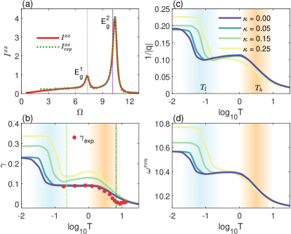
Figure 2: Panel (a): $I^{xx}$ and $I^{xx}_{\textmd{exp}}$ are, respectively, the strMC simulated Raman intensity and the experimental intensity from Ref. Sandilands et al. (2015) at $T=0.22$ and $\kappa=0$. By fitting $I^{xx}$ to the experimental intensity $I^{xx}_{\textmd{exp}}$, the best-fit model parameters are obtained: $\omega_{\Gamma}=[7.31,10.10]$, $\lambda_{\Gamma}=[0.25,0.52]$, $\mu_{\Gamma}=[0.38,1.00]$, $\nu=-0.63$. Panels (b-d): The temperature dependence of the $E_{g}^{2}$ peak curve parameters obtained from the asymmetric Lorentzian fitting: $1/|q|$, $\gamma$ and $\omega^{\textmd{r}en}$. $T_{l}$ and $T_{h}$ are two crossover temperatures. In panel (b), the computed $\gamma$ has been offset by a background line width obtained at $T=10^{1.5}$). This background line width mainly originates from the artificial broadening $\delta_{\textmd{ph}}$ as shown in Sec. D of SM. The red dots are experimental line width $\gamma_{\textmd{exp}}$, obtained from Ref. Sandilands et al. (2015). The two green vertical dashed lines in (e) indicate $T=5$ K and 150 K. The unit conversion we use here is $J\approx 23$ K.

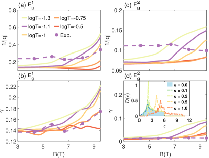
Figure 3: The magnetic field dependence of curve parameters $1/|q|$ and $\gamma$ of two phonon peaks $E_{g}^{1}$ and $E_{g}^{2}$ in the computed Raman spectrum are shown in (a,b) and (c,d), respectively. The purple dots denote experimental data from Ref. Wulferding et al. (2020) measured at $T=2$ K, i.e. log$T=-1.1$. The corresponding theoretical curve is also colored purple. The line width $\gamma$ has been offset by the background contribution (see caption of Fig. 2 for the reasoning). The inset of (b) shows the density of state of Majorana fermions at various $\kappa$ Feng et al. (2020). The conversion from $\kappa$ in the unit of $J$ to magnetic field $B$ in the unit of Tesla follows from Kitaev (2006): $\kappa=\frac{(\mu_{B}B)^{3}}{\Delta_{\textmd{flux}}^{2}}$, $\mu_{B}$ is the Bohr magneton and $\Delta_{\textmd{flux}}=0.27J$ is the flux energy, and $J\approx 23$ K.

Numerical results.— With the developed formalism at hand, we now study the temperature evolution of the Raman spectrum and its $\kappa$ dependence with the focus on the Fano lineshape. The thermodynamic average of the Raman correlation function over different flux configurations is computed numerically by using the strMC method Feng et al. (2021); Feng (2022) on a lattice size of $N_{1}=N_{2}=25$. We will focus on the $xx$-scattering geometry, in order to compare with the experiment, and assume $\delta_{\textmd{ph}}=0.15$.

To begin with, as shown in Fig. 2(a), we first fit the computed Raman intensity $I^{xx}(\Omega)$ to the experimental Raman intensity $I^{xx}_{\textmd{exp}}(\Omega)$ obtained from Ref. Sandilands et al. (2015), by tuning the adjustable model parameters {$\omega_{\Gamma},\lambda_{\Gamma},\mu_{\Gamma},\nu$}, whose best-fit values are written in the caption of Fig. 2. $I^{xx}(\Omega)$ is obtained by using Eq. (13) and evaluated at $T=0.22$ and $\kappa=0$. The details of the fitting procedure and justification of the uniqueness of the fitting parameters, after eliminating the overall scaling degree of freedom by setting $\mu_{E_{g}^{2}}=1$, are described in Sec. E of SM. Remarkably, the best-fit parameter $\lambda_{E_{g}^{2}}=0.52$ yields an estimation of the spin-phonon coupling to be $0.52\times\!\sqrt{6}\!=\!1.3J$, (with $\!\sqrt{6}$ being the norm of the bilinear $\Sigma_{\Gamma m}$ in Eq. (2)), comparable to the first principle calculation of magnetoelastic coupling $\approx 4J$ given in Ref. Kaib et al. (2021).

Next, with the fixed model parameters obtained above, we compute the evolution of the phonon Raman response by changing the temperature and the strength of $\kappa$. To quantitatively characterize the phonon peaks, we fit them to the asymmetric Lorentzian curve: $I(\Omega)=I_{0}\left[q\gamma+\left(\Omega-\omega^{\textmd{ren}}\right)\right]^{2}/[\gamma^{2}+\left(\Omega-\omega^{\textmd{ren}}\right)^{2}]$, where $1/q$ is the asymmetry factor, $\gamma$ is the half width at half maxima which is referred to as line width hereafter, $\omega^{\textmd{r}en}$ is the renormalized peak position and $I_{0}$ is the peak intensity.

The temperature evolution of curve parameters $\{1/|q|,\gamma,\omega^{\textmd{r}en}\}$ of the $E_{g}^{2}$ peak for various $\kappa$ is shown in Fig. 2 (b-d). As mentioned above, all curve parameters display a two-stage change with temperature. Two crossover temperatures, namely $T_{l}$ (in blue shaded area) and $T_{h}$ (in orange shaded area), correspond, respectively, to the flux proliferation temperature and the major fermionic excitation temperature Feng et al. (2020); Nasu et al. (2015); Feng et al. (2021). In the $T_{l}$ region, the curve parameters $\{1/q,\gamma,\omega^{\textmd{r}en}\}$ decrease significantly, which shows that they are sensitive to the emergent disorder from proliferated $Z_{2}$ fluxes. Also, the crossover temperature $T_{l}$ shows apparent $\kappa$ dependence, which reflects the increase of the flux gap energy with $\kappa$ Feng et al. (2020); Lahtinen (2011). In the $T_{h}$ region, further decrease of the curve parameters is due to Pauli exclusion principle of fermionic statistics. In Fig. 2(b), we also compare the experimental peak width $\gamma_{exp}$ obtained in Ref. Sandilands et al. (2015) with the computed $\gamma$. Remarkably, in the temperature region between 5 K and 150 K we find a good agreement between them. This result indicates that the source of anomalous peak width observed in Ref. Sandilands et al. (2015) can indeed be explained by spin-phonon coupling within our theoretical framework. Another noticeable result in Fig. 2(b-d) is that at the lowest temperature, the curve parameters become larger with increasing $\kappa$. This is because, as magnetic field increases, more Majorana fermions become energetically comparable with the phonon modes (see the inset of Fig. 3(d)), and participate in the spin-phonon scattering. So the curve parameters become bigger.

The magnetic field dependence of $\{1/|q|,\gamma\}$ of $E_{g}^{1}$ and $E_{g}^{2}$ peak for various temperatures in the $T_{l}$ region is shown in Fig. 3. The conversion from $\kappa$ to external field $B$ is presented in the caption, where the field direction is assumed to be $[111]$ for simplicity. We can see a clear trend in both peaks that, for a larger temperature in the $T_{l}$ region, the curve parameters start to increase at a larger magnetic field. This is because $Z_{2}$ flux gap energy is proportional to $\kappa$; thus as the temperature becomes larger, $Z_{2}$ fluxes require a higher magnetic field to be gapped out, after which the disorder introduced by $Z_{2}$ fluxes becomes weaker and the Fano effects becomes stronger. So the curve parameters start to increase at a larger field.

The computed curve parameters can be compared with the low-temperature experimental from Ref.Wulferding et al. (2020) and Ref. Sahasrabudhe et al. (2020). The data from Ref.Wulferding et al. (2020) is shown in Fig. 3 in the magnetic field region $B=3\sim 9T$ containing the putative QSL phase. Remarkably, in Fig. 3(a-b) there is a discernible increase in the parameters $\{1/|q|,\gamma\}$ in $E_{g}^{1}$ peak, whose magnitude is comparable with the theoretical increase. Our results also suggest that if the increase of the curve parameters at higher temperatures starts at higher fields, then this observation is consistent with the behaviour of the $Z_{2}$ fluxes. In Fig. 3(c-d), the experimental field dependence of the $E_{g}^{2}$ peak curve parameters remains featureless. This could be attributed to the fact that the $E_{g}^{2}$ phonon has higher energy than $E_{g}^{1}$, thus it is less sensitive to the increased population of fermionic modes from the increased field.

Conclusion. – We have constructed a theory to describe the Raman scattering of the spin-phonon coupled Kitaev system. Based on this theory, we systematically compute the Raman spectrum and explore the temperature evolution and the magnetic field dependence of the phonon peaks in Raman spectrum, which are consistent with the Raman scattering experiment in $\alpha\textmd{-RuCl}_{3}$. Our theory clarifies the mechanism of how spin-phonon coupling generates Fano lineshapes, and also offers an estimate of the spin-phonon coupling by model fitting. These results open the possibility of experimentally identifying the effects of fractionalized excitations of QSL hidden in the Fano lineshapes of phonon Raman peaks.

Acknowledgments: The authors are thankful to Ken Burch, Jia-Wei Mei, Joji Nasu, Kenya Ohgushi, Thuc T Mai, Luke Sandilands, Yiping Wang, Yang Yang, Mengxing Ye, Shuo Zhang and especially Dirk Wulferding for valuable discussions. The work was supported by the U.S. Department of Energy, Office of Basic Energy Sciences under Award No. DE-SC0018056. N.B.P. acknowledges the hospitality of Aspen Center of Physics.

Supplementary Material

Appendix A A. The irreducible representations of the phonon modes

In the main text, we have introduced the phonon Hamiltonian $H_{\textmd{ph}}$. Its normal vibration modes will be solved by group theory. The point group we consider here is $D_{3d}$, which is the symmetry shared by both the Kitaev model You et al. (2012) and a single layer of $\alpha$-$\textmd{RuCl}_{3}$ Li et al. (2019). The invariance of the phonon Hamiltonian under the group operations requires $[H_{\mathrm{ph}},D_{3d}]=0$. Then, to obtain the eigenmodes of $H_{\textmd{ph}}$, we apply the following theorem:

Theorem 1.

If a Hamiltonian $H$ is invariant under the group $G$, i.e., $[G,H]=0$, then the irreducible representation of $G$ forms the basis of the eigensubspace of $H$; and the energy of multidimensional irreducible representation is degenerate.

The proof can be found in Ref. Feng (2022); Inui et al. (1996) . Applying this theorem to the current work, we can see that in the symmetry group $D_{3d}$, the irreducible representation of normal vibration modes $u_{\Gamma m}$ forms the eigensubspace of $H$, and the energy of 2-dimensional irreducible representation $E_{g}$ is degenerate, i.e., $H_{\textmd{ph}}u_{\Gamma m}=\omega_{\Gamma}u_{\Gamma m}$, where $\Gamma=E_{g}$.

As introduced in the main text, the general form of the phonon Hamiltonian can be written as $H_{\textmd{ph}}=H_{\textmd{ph}}(p_{i}(\mathbf{r}),q_{i}(\mathbf{r}))$, where $q_{i}(\mathbf{r})=(x_{1},y_{1},z_{1},\ldots,x_{8},y_{8},z_{8})_{\bf r}$ describes the displacement fields in a unit cell located at $\mathbf{r}$, which contains two Ru³⁺ and six Cl^- ions. $p_{i}(\mathbf{r})$ is the corresponding momentum. The vibration eigenmodes at the center of the Brillouin zone is classified according to the irreducible representations (irreps) of $D_{3d}$: $\Gamma=2A_{1g}+2A_{2g}+4E_{g}+A_{1u}+3A_{2u}+4E_{u}$, among which the Raman active modes are $\Gamma_{R}=2A_{1g}+4E_{g}$ Guizzetti et al. (1979); Li et al. (2019). Assuming that the phonon potential energy can be expanded as $V(q_{i})=V_{0}+\frac{1}{2}\sum_{i,j=1}^{24}\left.\frac{\partial^{2}V}{\partial{q}_{i}\partial{q}_{j}}\right|_{0}{q}_{i}{q}_{j}+\cdots$, then a vibration eigenmode can be written as a linear combination of the displacement fields: $u_{\Gamma m}(\mathbf{r})=\sum_{i}u_{\Gamma m,i}{q}_{i}(\mathbf{r})$, where $\Gamma$ denotes the irreps of dimension $m$. As mentioned in the main text, we will drop the $\mathbf{r}$ dependence due to long wave approximation. Then, applying linear representation theory of finite groups Inui et al. (1996); Dummit and Foote (2004); Serre (1977) , we obtain the explicit form of these vibration modes and show the Raman active ones here:

$$E^{1}_{g}:\left\{\begin{array}[]{l}+0.07x_{3}-0.47z_{3}-0.07x_{4}+0.47z_{4}-0.27x_{5}-0.11y_{5}-0.23z_{5}+0.27x_{6}\\ \quad+0.11y_{6}+0.23z_{6}+0.27x_{7}-0.11y_{7}+0.23z_{7}-0.27x_{8}+0.11y_{8}-0.23z_{8},\\ +0.33y_{3}-0.33y_{4}-0.11x_{5}-0.14y_{5}+0.40z_{5}+0.11x_{6}\\ \quad+0.14y_{6}-0.40z_{6}-0.11x_{7}+0.14y_{7}+0.40z_{7}+0.11x_{8}-0.14y_{8}-0.40z_{8}\end{array}\right.$$ (A5)

$$E^{2}_{g}:\left\{\begin{array}[]{l}\frac{1}{\sqrt{2}}(y_{1}-y_{2})\\ \frac{1}{\sqrt{2}}(-x_{1}+x_{2})\end{array}\right.$$ (A8)

$$E^{3}_{g}:\left\{\begin{array}[]{l}-0.57x_{3}-0.06z_{3}+0.57x_{4}+0.06z_{4}+0.11x_{5}-0.27y_{5}-0.03z_{5}-0.11x_{6}\\ \quad+0.27y_{6}+0.03z_{6}-0.11x_{7}-0.27y_{7}+0.03z_{7}+0.11x_{8}+0.27y_{8}-0.03z_{8},\\ +0.04y_{3}-0.04y_{4}-0.27x_{5}+0.42y_{5}+0.05z_{5}+0.27x_{6}\\ \quad-0.42y_{6}-0.05z_{6}-0.27x_{7}-0.42y_{7}+0.05z_{7}+0.27x_{8}+0.42y_{8}-0.05z_{8}\end{array}\right.$$ (A13)

$$E^{4}_{g}:\left\{\begin{array}[]{l}-0.34z_{3}+0.34z_{4}+0.35x_{5}+0.20y_{5}-0.17z_{5}-0.35x_{6}\\ \quad-0.20y_{6}+0.17z_{6}-0.35x_{7}+0.20y_{7}+0.17z_{7}+0.35x_{8}-0.20y_{8}-0.17z_{8},\\ -0.47y_{3}+0.47y_{4}+0.20x_{5}+0.12y_{5}+0.29z_{5}-0.20x_{6}\\ \quad-0.12y_{6}-0.29z_{6}+0.20x_{7}-0.12y_{7}+0.29z_{7}-0.20x_{8}+0.12y_{8}-0.29z_{8}\end{array}\right.$$ (A18)

$$A^{1}_{1g}:\begin{array}[]{l}-\frac{1}{\sqrt{2}}z_{1}+\frac{1}{\sqrt{2}}z_{2}\end{array}$$ (A20)

$$A^{2}_{1g}:-\frac{1}{\sqrt{6}}x_{3}+\frac{1}{\sqrt{6}}x_{4}-\frac{1}{2\sqrt{6}}x_{5}+\frac{1}{2\sqrt{2}}y_{5}+\frac{1}{2\sqrt{6}}x_{6}-\frac{1}{2\sqrt{2}}y_{6}+\frac{1}{2\sqrt{6}}x_{7}+\frac{1}{2\sqrt{2}}y_{7}$$ (A21)

$$\qquad\qquad-\frac{1}{2\sqrt{6}}x_{8}-\frac{1}{2\sqrt{2}}y_{8},$$

where the atom labeling convention followed is shown in Fig. S1.

To illustrate the phonon modes solutions shown above, we consider a concrete example of phonon Hamiltonian $H_{\textmd{ph}}=\sum_{i}\frac{p_{i}^{2}}{2m_{i}}+V(q_{i})$, where $m_{i}$ is the mass of the i-th vibrating coordinate, and the potential energy is quadratic as introduced above: $V(q_{i})=\frac{1}{2}\sum_{i,j=1}^{24}\left.\frac{\partial^{2}V}{\partial{q}_{i}\partial{q}_{j}}\right|_{0}{q}_{i}{q}_{j}$. Then $H_{\textmd{ph}}$ is rewritten as:

$$H_{\textmd{ph}}=\sum_{ij}\left[\frac{1}{2}\tilde{p}_{i}\mathbb{1}_{ij}\tilde{p}_{j}+\frac{1}{2}\tilde{q}_{i}K_{ij}\tilde{q}_{j}\right],$$ (A22)

where $\tilde{p}_{i}=\frac{p_{i}}{\sqrt{m_{i}}}$, $\tilde{q}_{i}=\sqrt{m_{i}}q_{i}$ are conjugate canonical coordinates, and $K_{ij}=\left.\frac{\partial^{2}V}{\partial{q}_{i}\partial{q}_{j}}\right|_{0}\cdot\frac{1}{\sqrt{m_{i}m_{j}}}$. So, if this phonon Hamiltonian $H_{\textmd{ph}}$ satisfies the $D_{3d}$ symmetry (mainly the potential energy term, since the kinetic energy term is isotropic), then the quadratic potential energy $K_{ij}$ will be block-diagonalized by the modes $u_{\Gamma m}$ listed above, with each block being labelled by the irreducible representation $\Gamma$. It is then clear that the modes $u_{\Gamma m}$ indeed give the correct eigen vibration modes for the phonon Hamiltonian $H_{\textmd{ph}}$. The following steps are generic: $H_{\textmd{ph}}=\sum_{\Gamma m}\frac{1}{2}\omega_{\Gamma}\left[\frac{P_{\Gamma m}^{2}}{\omega_{\Gamma}}+\omega_{\Gamma}u^{2}_{\Gamma m}\right]=\sum_{\Gamma m}\omega_{\Gamma}(b_{\Gamma m}^{\dagger}b_{\Gamma m}+\frac{1}{2})$, where $\omega^{2}_{\Gamma}$ is the eigenvalue of $K$, $P_{\Gamma m}=\sum_{i}u_{\Gamma m,i}\tilde{p}_{i}$ and $u_{\Gamma m}=\sum_{i}u_{\Gamma m,i}\tilde{q}_{i}$ are conjugate canonical coordinates of the eigenmodes, and $b_{\Gamma m}^{\dagger},b_{\Gamma m}$ are the corresponding creation and annihilation operators.

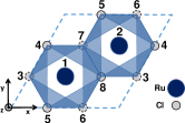
Figure S1: Unit cell of $\alpha-$RuCl₃ with labeled ions.

Next we compare the above phonon modes with the results from the density functional theory (DFT) calculations Li et al. (2019) with a goal to identify the two low-energy $E_{g}$ modes among the four pairs of $E_{g}$ modes identified by DFT. By looking at the major dominant vibrating components and their relative directions on each Ru³⁺ and Cl^- ions, we conclude that the low-energy modes $E_{g}^{1}$ and $E_{g}^{2}$ modes are those given by Eq. (A5) and Eq. (A8), respectively. Note that the $E^{2}_{g}$ mode Eq. (A8) only involves vibrations of $\textmd{Ru}^{3+}$ ions. If only the vibration of $\textmd{Ru}^{3+}$ ions are considered Metavitsiadis et al. (2021), under $D_{3d}$ constraint the phonon modes decompose as $\Gamma_{Ru}=A_{1g}+E_{g}+A_{2u}+E_{u}$, where $A_{2u}+E_{u}$ are the acoustic modes, and $E_{g}=E_{g}^{2}$ and $A_{1g}$ modes are those given by Eq. (A8) and Eq. (A20). The DFT calculations Li et al. (2019) suggest that $E_{g}^{2}$ has higher energy than $E^{1}_{g}$ mode Eq. (A5), in which vibrations are predominantly from $\textmd{Cl}^{-1}$ ions whose mass is smaller. This indicates that the corresponding stiffness is also smaller.

Finally, we give the matrix representations of the $D_{3d}$ group in the basis of the $E_{g}$ phonons Eq.(A5)-(A18), i.e. $\bra{u_{E_{g},m}}D_{3d}\ket{u_{E_{g},m^{\prime}}}$, where $m,m^{\prime}=1$, 2. It suffices to just show the result of the two generators of $D_{3d}$: $S_{6}$ the 6-fold rotoreflection, and $C^{\prime}_{2}$ the 2-fold rotation around the $y$-axis in Fig. S1, while the representations of other group elements can be obtained via group multiplication. In the $E_{g}$ phonon sector,

$$S_{6}=\left[\begin{array}[]{cc}-1/2&\sqrt{3}/2\\ -\sqrt{3}/2&-1/2\end{array}\right],\quad C^{\prime}_{2}=\left[\begin{array}[]{cc}1&0\\ 0&-1\end{array}\right].$$ (A27)

This $E_{g}$ representation given by the phonon sector is exactly the same as the $E_{g}$ representation given by the other two sectors, namely the spin bilinear products $\Sigma_{\Gamma m}$ and the Raman polarization tensors $R_{\Gamma m}^{\mu\nu}E_{\textmd{in}}^{\mu}E_{\textmd{out}}^{\nu}$. This guarantees that the coupling Hamiltonians built by the inner product of the irreps from any two of the aforementioned three sectors are invariant under the $D_{3d}$ transformations. More specifically, the transformation of the physical fields involved in the above three sectors is given by the following. For a given element $g\in D_{3d}$,

$$\vec{\sigma}(\mathbf{r}) \to\vec{\sigma}\,^{\prime}(\mathbf{r}^{\prime})=O_{g}^{\mkern-1.5mu\mathsf{T}}\vec{\sigma}(O_{g}\mathbf{r}),$$ (A28)

$$\vec{E}(\mathbf{r}) \to\vec{E}\,^{\prime}(\mathbf{r}^{\prime})=O_{g}^{\mkern-1.5mu\mathsf{T}}\vec{E}(O_{g}\mathbf{r}),$$ (A29)

$$\vec{q}\,(\mathbf{r}) \to\vec{q}\,^{\prime}(\mathbf{r}^{\prime})=O_{g}^{\mkern-1.5mu\mathsf{T}}\vec{q}\,(O_{g}\mathbf{r}).$$ (A30)

where $O_{g}$ is an operation of $g$ on a 3D vector. Then, the transformation of the spin bilinear products $\Sigma_{\Gamma m}(\mathbf{r})$, the Raman polarization tensors $R_{\Gamma m}^{\mu\nu}E^{\mu}_{\textmd{in}}(\mathbf{r})E_{\textmd{out}}^{\nu}(\mathbf{r})$, and the phonon sector $u_{\Gamma m,i}q_{i}(\mathbf{r})$ can be derived. Based on this, the $D_{3d}$ invariance of the coupling Hamiltonians Eq. (2) Eq. (4) Eq. (12), and the $E_{g}$ representation Eq. (A27) can be explicitly verified.

Appendix B B. The symmetry decomposition of the Loudon-Fleury Raman operator

As introduced in the main text, the Loudon-Fleury Raman operator has $D_{3d}$ symmetry. To explicitly see this symmetry, here we show the explicit decomposition of this operator into the irreducible representations of $D_{3d}$.

To begin with, we first introduce the irreducible representations of the Raman tensors Kroumova et al. (2003):

$$R_{A_{1g}}=\left[\begin{array}[]{ccc}a&0&0\\ 0&a&0\\ 0&0&b\end{array}\right],\quad R_{E_{g},1}=\left[\begin{array}[]{ccc}c&0&d\\ 0&-c&0\\ d&0&0\end{array}\right],\quad R_{E_{g},2}=\left[\begin{array}[]{ccc}0&-c&0\\ -c&0&d\\ 0&d&0\end{array}\right].$$ (B10)

In the following derivative, we use $a=c=1,b=d=0$ since we consider only 2D component of electromagnetic field.

Then as introduced in the main text, the Raman operator of this spin-phonon coupled Kitaev system is described by ${\mathcal{R}}$=$\sum_{\mu\mu^{\prime}}\left({\mathcal{R}}^{\mu\mu^{\prime}}_{\textmd{em-ph}}+{\mathcal{R}}^{\mu\mu^{\prime}}_{\textmd{em-s}}\right)E^{\mu}_{\textmd{in}}E^{\mu^{\prime}}_{\textmd{out}}$, and the coupling of electromagnetic wave to spin is described by Loudon-Fleury operator ${\mathcal{R}}^{\mu\mu^{\prime}}_{\textmd{em-s}}=\nu\sum_{\alpha,{\bf r}\in A}{\bf M}_{\alpha}^{\mu}{\bf M}_{\alpha}^{\mu^{\prime}}\sigma_{\bf r}^{\alpha}\sigma_{{\bf r}+{\bf M}_{\alpha}}^{\alpha}$. Now we are ready to decompose this tensor into the irreducible representations in Eq. (B10): $\mathcal{R}^{\mu\mu^{\prime}}_{\textmd{em-s}}=\sum_{\Gamma m}\alpha_{\Gamma m}R^{\mu\mu^{\prime}}_{\Gamma m}$, where $R_{\Gamma m}^{\mu\nu}$ are the Raman tensors. Using their orthogonality relations, the coefficient $\alpha_{\Gamma m}$ are obtained: $\alpha_{\Gamma m}=\frac{1}{2}\operatorname{Tr}[R_{\Gamma m}^{\ {\mkern-1.5mu\mathsf{T}}}\cdot\mathcal{R}_{\textmd{em-s}}]$, where the dot is the matrix product on $\mu\mu^{\prime}$ indices. Then the symmetry decomposition of ${\mathcal{R}}_{\textmd{em-s}}$ according to $D_{3d}$ can be written as $\mathcal{R}^{\mu\mu^{\prime}}_{\textmd{em-s}}=\nu\sum_{\Gamma m}\Sigma_{\Gamma m}R^{\mu\mu^{\prime}}_{\Gamma m}$. Since $\left[{\mathcal{R}}_{\textmd{em-s},A_{g}},H_{\textmd{s}}\right]=0$, and thus only $\Gamma=E^{1}_{g}$ and $\Gamma=E^{2}_{g}$ channels contribute into the Raman response with the Raman operator given by ${\mathcal{R}}_{\textmd{em-s}}^{\mu\mu^{\prime}}=\nu\sum_{m}\Sigma_{E_{g},m}R^{\mu\mu^{\prime}}_{E_{g},m}$.

Appendix C C. Perturbative calculation of the Raman response in the spin-phonon coupled Kitaev system

The spin-dependent phonon Raman scattering intensity is calculated as follows. There are two channels for the Raman scattering response, the phonon and the spin, so the Raman operator can be written as

$${\mathcal{R}}={\mathcal{R}}_{\textmd{em-ph}}+{\mathcal{R}}_{\textmd{em-s}},$$ (C1)

where ${\mathcal{R}}_{\textmd{em-ph}}=\sum_{\Gamma,m}\mu_{\Gamma}R_{\Gamma m}^{\mu\mu^{\prime}}u_{\Gamma m}E^{\mu}_{\textmd{in}}E^{\mu^{\prime}}_{\textmd{out}}$ and ${\mathcal{R}}_{\textmd{em-s}}=\nu\sum_{m}R^{\mu\mu^{\prime}}_{E_{g},m}\Sigma_{E_{g},m}E^{\mu}_{\textmd{in}}E^{\mu^{\prime}}_{\textmd{out}}$, respectively, denote the coupling of electromagnetic field of light to phonons and spins as introduced in the main text.

In the simplest case, when the spins and phonons are decoupled, the general expression for the intensity is expressed as

$$I(\Omega)\!=\!\int\!dt~{}e^{i\Omega t}\langle T_{t}\mathcal{R}(t)\mathcal{R}(0)\rangle,$$ (C2)

where $I(t)=\left\langle T_{t}\mathcal{R}(t)\mathcal{R}(0)\right\rangle$ is the time-ordered Raman correlation function. It is also convenient to introduce the retarded Raman correlation function, which is also known as the Raman susceptibility:

$$\chi(\Omega)=-i\int\mathrm{d}te^{i\Omega t}\Theta(t)\langle\left[\mathcal{R}(t),\mathcal{R}(0)\right]\rangle.$$ (C3)

The Raman intensity $I(\Omega)$ and the Raman susceptibility $\chi(\Omega)$ are related via the fluctuation-dissipation theorem:

$$I(\Omega)=-\frac{2}{1-e^{-\beta\Omega}}\operatorname{Im}\chi(\Omega).$$ (C4)

Since we are interested in the Raman scattering at finite temperatures, we will work in the Matsubara formalism, in which the Matsubara correlation function of Raman operators is given by $\mathcal{I}(\tau)=-\left\langle T_{\tau}\mathcal{R}(\tau)\mathcal{R}(0)\right\rangle$ and the Fourier transform can be written as

$$\mathcal{I}(i\Omega_{n})=-\int\mathrm{d}\tau e^{i\Omega_{n}\tau}\left\langle T_{\tau}\mathcal{R}(\tau)\mathcal{R}(0)\right\rangle.$$ (C5)

After analytical continuation $i\Omega_{n}\to\Omega+i\delta$, we directly obtain the retarded correlation function, i.e. the Raman susceptibility, $\chi(\Omega)=\mathcal{I}({i\Omega_{n}})|_{i\Omega_{n}\rightarrow\Omega+i\delta}$. So in the following derivation, we only need to focus on evaluating the Matsubara correlation function of the Raman operators, $\mathcal{I}(i\Omega_{n})$.

Applying this mechanism, we first compute the Raman response of the decoupled phonon and spin subsystems. In this case, $\mathcal{I}_{0}=\mathcal{I}_{\textmd{em-ph}}+\mathcal{I}_{\textmd{em-s}}$. The first term describes the pure phonon Raman scattering:

$$\mathcal{I}_{\textmd{em-ph}}^{\mu\mu^{\prime}}(i\Omega_{n})=\sum_{\Gamma m}\mu^{2}_{\Gamma}\left(R_{\Gamma m}^{\mu\mu^{\prime}}\right)^{2}\mathcal{D}^{(0)}_{\Gamma\Gamma,mm}(i\Omega_{n})$$ (C6)

where the scattering geometry $\mu\mu^{\prime}$ has been explicitly specified, $\mu_{\Gamma}$ is the photon-phonon coupling constant in the $\Gamma$ irrep and $R_{\Gamma m}^{\mu\mu^{\prime}}$ is the Raman polarization tensor defined by Eq. (B10) and $\mathcal{D}^{(0)}_{\Gamma m,\Gamma^{\prime}m^{\prime}}(i\omega_{n})=\frac{2\omega_{\Gamma}}{\left(i\omega_{n}\right)^{2}-\omega_{\Gamma}^{2}}\delta_{\Gamma\Gamma^{\prime}}\delta_{mm^{\prime}}$ is the bare phonon propagator. The corresponding Raman response is simply given by a set of delta functions at the bare phonon frequencies $\omega_{\Gamma}$.

The second term comes from the magnetic Raman scattering:

$$\mathcal{I}_{\textmd{em-s}}^{\mu\mu^{\prime}}(i\Omega_{n})=-\int_{0}^{\beta}\mathrm{d}\tau e^{i\Omega_{n}\tau}\langle T_{\tau}\mathcal{R}_{\textmd{em-s}}^{\mu\mu^{\prime}}(\tau)\mathcal{R}_{\textmd{em-s}}^{\mu\mu^{\prime}}(0)\rangle.$$ (C7)

The spin bilinear operator can be rewritten using the Majorana fermion representation of the spin: $\sigma_{j}^{\alpha}=ib_{j}^{\alpha}c_{j}$, and then transformed into the basis of the fermionic eigenmodes Feng et al. (2021). Explicitly, the correlation function of the spin Raman operators is written as a general form of $-\left\langle T_{\tau}\left(\mathbf{B}^{\dagger}\tilde{\Lambda}\mathbf{B}\right)(\tau)\left(\mathbf{B}^{\dagger}\tilde{\Lambda}\mathbf{B}\right)(0)\right\rangle$, where $\mathbf{B}^{\dagger}=\left[\beta_{1}^{\dagger},\cdots\beta_{N}^{\dagger},\beta_{1},\cdots\beta_{N}\right]$ is the vector of the Bogoliubov quasiparticles, and $\tilde{\Lambda}$ is a symmetrized coupling matrix, whose entries are the coupling vertices between two fermion eigenmodes and the photons. Since the fermionic eigenmodes are different for different flux configurations, coupling matrix $\tilde{\Lambda}$ is a function of $Z_{2}$ gauge fluxes. For a given temperature, the thermodynamic average over different flux configurations is evaluated by stratified Monte Carlo (strMC) method, which was introduced and applied to acoustic phonon dynamics in Ref. Feng et al. (2021); Feng (2022).

Finally, $\mathcal{I}_{\textmd{em-s}}^{\mu\mu^{\prime}}(i\Omega_{n})$ is evaluated as

$$\mathcal{I}_{\textmd{em-s}}^{\mu\mu^{\prime}}(i\Omega_{n})\sim\operatorname{Tr}\left[{\mathcal{G}}_{1}(i\omega_{n})\tilde{\Lambda}{\mathcal{G}}_{1}^{*}(i\Omega_{n}-i\omega_{n_{1}})\tilde{\Lambda}+{\mathcal{G}}_{2}(i\omega_{n})\tilde{\Lambda}{\mathcal{G}}_{2}(i\Omega_{n}-i\omega_{n_{1}})\tilde{\Lambda}^{\mkern-1.5mu\mathsf{T}}\right],$$ (C8)

which appears as a fermionic loop diagram shown in Fig. S3(b). Here, the indices $\mu\mu^{\prime}$ are contained inside $\tilde{\Lambda}$, ${\operatorname{Tr}}[...]$ sums over the Matsubara frequencies $i\omega_{n_{1}}$ as $T\sum_{n_{1}}$, and the matrix form of the Matsubara Green’s functions is given by:

$$\mathcal{G}_{1}\left(i\omega_{n}\right) \equiv\left[\begin{array}[]{ll}\bar{g}\left(i\omega_{n}\right)&O\\ O&g\left(i\omega_{n}\right)\end{array}\right],$$ (C11)

$$\mathcal{G}_{2}\left(i\omega_{n}\right) \equiv\left[\begin{array}[]{ll}O&g\left(i\omega_{n}\right)\\ \bar{g}\left(i\omega_{n}\right)&O\end{array}\right],$$ (C14)

where, $g_{i}\left(i\omega_{n}\right)=\frac{1}{i\omega_{n}-\epsilon_{i}}$ and $\bar{g}_{i}\left(i\omega_{n}\right)=\frac{1}{i\omega_{n}+\epsilon_{i}}$. The spectrum of $\mathcal{I}_{\textmd{em-s}}^{\mu\mu^{\prime}}$ appears as a magnetic continuum, which has been studied at length in the literature Knolle et al. (2014a); Nasu et al. (2016); Rousochatzakis et al. (2019) and will not be repeated here.

The main goal of this work is to study the Raman response in the spin-phonon coupled Kitaev system described by the Hamiltonian (1) in the main text. The presence of the spin-phonon interaction (Eq.(2) in the main text) leads to the Raman vertex renormalization due to the final-state interactions. In the interaction picture, the general expression of the Raman correlation function in the presence of the spin-phonon coupling is given by

$$I(t)=\langle T_{t}\mathcal{R}(t)\mathcal{R}(0)e^{-i\int\mathrm{d}t^{\prime}H_{\textmd{s-ph}}(t^{\prime})}\rangle,$$ (C15)

where $S=e^{-i\int\mathrm{d}t^{\prime}H_{\textmd{s-ph}}(t^{\prime})}$ is the dubbed $S$-matrix. Correspondingly, at finite temperature $\mathcal{I}(\tau)=-\left\langle T_{\tau}\mathcal{R}(\tau)\mathcal{R}(0)e^{-\int_{0}^{\beta}\mathrm{d}\tau^{\prime}H_{\textmd{s-ph}}(\tau^{\prime})}\right\rangle$ gives the Matsubara correlation function of the Raman operator in the spin-phonon coupled Kitaev model. Treating the coupling $H_{\textmd{s-ph}}$ perturbatively and using the $S$-matrix expansion Mahan (2013), we obtain:

$$\mathcal{I}(\tau)=-\sum_{k=0}^{\infty}(-1)^{k}\prod_{i}^{k}\int_{0}^{\beta}\mathrm{d}\tau_{i}\left\langle T_{\tau}\mathcal{R}(\tau)\mathcal{R}(0)\prod_{i}^{k}H_{\textmd{s-ph}}(\tau_{i})\right\rangle$$ (C16)

where only connected different graphs are summed. At the order of $k=0$, this expression corresponds to the simple spin-phonon decoupled case, as described above.

Figure S2: The Feynman diagrams of the phonon Raman vertices: (a) $\mu_{\Gamma}R_{\Gamma m}$ (b) $\mathcal{P}_{\Gamma m,L}$ (c) $\mathcal{P}_{\Gamma m,R}$.

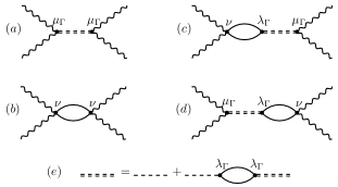
Figure S3: The Feynman diagrams of the Raman intensity shown in Eq. (C26). (a) the phonon channel with a propagator renormalized by the spin-phonon interaction (Eq.(2) in the main text), (b) the spin channel, (c)-(d) the phonon-spin mixed channel with the spin-dependent phonon Raman vertices $\mathcal{P}_{\Gamma m,L}$, $\mathcal{P}_{\Gamma m,R}$. Panel (e) shows the Dyson’s equation for the phonon propagator.

At the order of $k=1$, contribution can be explicitly written as

$$\mathcal{I}_{1}^{\mu\mu^{\prime}}(\tau) =\int_{0}^{\beta}\mathrm{d}\tau_{1}\left\langle T_{\tau}\mathcal{R}^{\mu\mu^{\prime}}(\tau)\mathcal{R}^{\mu\mu^{\prime}}(0)H_{\textmd{s-ph}}(\tau_{1})\right\rangle=\left\{\begin{array}[]{l}\int_{0}^{\beta}\mathrm{d}\tau_{1}\left\langle T_{\tau}\mathcal{R}^{\mu\mu^{\prime}}_{\textmd{em-s}}(\tau)\mathcal{R}^{\mu\mu^{\prime}}_{\textmd{em-ph}}(0)H_{\textmd{s-ph}}(\tau_{1})\right\rangle\\ \int_{0}^{\beta}\mathrm{d}\tau_{1}\left\langle T_{\tau}\mathcal{R}_{\textmd{em-ph}}^{\mu\mu^{\prime}}(\tau)\mathcal{R}^{\mu\mu^{\prime}}_{\textmd{em-s}}(0)H_{\textmd{s-ph}}(\tau_{1})\right\rangle\end{array}\right.$$ (C19)

$$=\left\{\begin{array}[]{l}\sum_{\Gamma,m,m^{\prime}}\mu_{\Gamma}\lambda_{\Gamma}R_{\Gamma m}^{\mu\mu^{\prime}}\int_{0}^{\beta}\mathrm{d}\tau_{1}\left\langle T_{\tau}\mathcal{R}^{\mu\mu^{\prime}}_{\textmd{em-s}}(\tau)\Sigma_{\Gamma m^{\prime}}(\tau_{1})u_{\Gamma m^{\prime}}(\tau_{1})u_{\Gamma m}(0)\right\rangle\\ \sum_{\Gamma,m,m^{\prime}}\mu_{\Gamma}\lambda_{\Gamma}R_{\Gamma m}^{\mu\mu^{\prime}}\int_{0}^{\beta}\mathrm{d}\tau_{1}\left\langle T_{\tau}u_{\Gamma m}(\tau)\Sigma_{\Gamma m^{\prime}}(\tau_{1})u_{\Gamma m^{\prime}}(\tau_{1})\mathcal{R}_{\textmd{em-s}}^{\mu\mu^{\prime}}(0)\right\rangle\end{array}\right.$$ (C22)

which contributes into the lowest order of the diagrams shown in (c)(d) respectively Fig. S3 (c-d). At this order, it gives to the spin-dependent phonon Raman vertices (first introduced in Moriya (1967); Suzuki and Kamimura (1973)), which describe the mixing term between the two channels and play the central role in generating the Fano lineshape. These two spin-dependent phonon Raman vertices, which are distinguished with notation left (L) and right (R), are given by

$$\mathcal{P}^{\mu\mu^{\prime}}_{\Gamma m,L}(\tau)=-\lambda_{\Gamma}\left\langle T_{\tau}\Sigma_{\Gamma m}(\tau)\mathcal{R}^{\mu\mu^{\prime}}_{\textmd{em-s}}(0)\right\rangle,$$

$$\mathcal{P}^{\mu\mu^{\prime}}_{\Gamma m,R}(\tau)=-\lambda_{\Gamma}\left\langle T_{\tau}\mathcal{R}^{\mu\mu^{\prime}}_{\textmd{em-s}}(\tau)\Sigma_{\Gamma m}(0)\right\rangle.$$ (C23)

The corresponding diagrams are shown in Fig. S2 (b-c). Combining $\mathcal{P}^{\mu\mu^{\prime}}_{\Gamma m,L}(\tau)$ and $\mathcal{P}^{\mu\mu^{\prime}}_{\Gamma m,R}(\tau)$ with the bare Raman vertex $R_{\Gamma m}^{\mu\mu^{\prime}}$, we define the renormalized left and right phonon Raman vertices as:

$${R^{\prime}}_{\Gamma m,L}^{\mu\mu^{\prime}}(\tau)=\mu_{\Gamma}R_{\Gamma m}^{\mu\mu^{\prime}}+\mathcal{P}^{\mu\mu^{\prime}}_{\Gamma m,L}(\tau),$$

$${R^{\prime}}_{\Gamma m,R}^{\mu\mu^{\prime}}(\tau)=\mu_{\Gamma}R_{\Gamma m}^{\mu\mu^{\prime}}+\mathcal{P}^{\mu\mu^{\prime}}_{\Gamma m,R}(\tau).$$ (C24)

With these renormalized phonon Raman vertices, the odd-$k$ terms and even-$k$ terms in the expansion Eq. (C16) are grouped together, and the summation naturally forms the series that is consistent with Dyson’s equation, which describes the renormalization of the phonon propagator:

$$\mathcal{D}_{\Gamma m,\Gamma^{\prime}m^{\prime}}=\left[[\mathcal{D}^{(0)}_{\Gamma m,\Gamma^{\prime}m^{\prime}}]^{-1}-\Pi_{\Gamma m,\Gamma^{\prime}m^{\prime}}\right]^{-1}$$ (C25)

described by Fig. S3 (e). Here, $\Pi_{\Gamma m,\Gamma^{\prime}m^{\prime}}(\tau)=-\lambda_{\Gamma}\lambda_{\Gamma^{\prime}}\left\langle T_{\tau}\Sigma_{\Gamma m}(\tau)\Sigma_{\Gamma^{\prime}m^{\prime}}(0)\right\rangle$ is the polarization bubble given by Eq.(3) of the main text. Its temperature and field dependence are discussed in the section. Then the final expression of the Raman correlation function can be obtained:

$$\mathcal{I}(\tau)=\mathcal{I}_{\textmd{em-s}}(\tau)+R^{\prime}_{L}(\tau)\cdot\hat{\mathcal{D}}(\tau)\cdot R^{\prime}_{R}(\tau),$$ (C26)

where the dot product is on the contraction of ($\Gamma,m$) indices. This result is summarized in Fig. S3 (a)-(d), where the diagrams (a),(c) and (d) are contained in the second term of the above expression. The renormalized phonon Raman vertices Eq. (C24) can be also written as $R^{\prime}_{\Gamma m}(\tau)=R_{\Gamma m}\left[\mu_{\Gamma}+\frac{\nu}{\lambda_{\Gamma}}\Pi_{\Gamma m,\Gamma m}(\tau)\right]$, when $\kappa=0$. In the frequency domain, the fermionic bubble gives the frequency-dependent renormalization of the phonon Raman coupling $\mu_{\Gamma}$, which eventually leads to the asymmetry of the phonon Raman peak.

Appendix D D. The polarization bubble and its influence on the phonon peaks

In this section, we will analyze the temperature and field dependence of the polarization bubble $\Pi_{\Gamma m,\Gamma^{\prime}m^{\prime}}=-\lambda_{\Gamma}\lambda_{\Gamma^{\prime}}\left\langle T_{\tau}\Sigma_{\Gamma m}(\tau)\Sigma_{\Gamma^{\prime}m^{\prime}}(0)\right\rangle,$ and discuss its effects on the shape of the phonon Raman peaks. As the $E_{g}^{1}$ and $E_{g}^{2}$ phonon peaks are energetically well separated Li et al. (2019), the off-diagonal components of $\Pi_{\Gamma m,\Gamma^{\prime}m^{\prime}}$ are negligible. Thus, we will focus only on the diagonal blocks of $\hat{\Pi}$, which are denoted as $\Pi_{mm^{\prime}}\equiv\Pi_{\Gamma m,\Gamma m^{\prime}}$.

In Fig. S4, we present the real and imaginary parts of $\Pi_{mm^{\prime}}$ (blue and red curves, respectively) as functions of frequency and temperature, computed by stratified Monte Carlo method (strMC) Feng et al. (2021); Feng (2022). Fig. S4(a-b) show the components of $\Pi_{mm^{\prime}}$ computed for $\kappa=0$ at temperatures $T=0.03$ and $T=1$, respectively. We can see that both at low ($T=0.03$) and high ($T=1$) temperatures $\Pi_{12}$ and $\Pi_{21}$ are negligibly small, which shows that the two degenerate phonon modes are indeed orthogonal. Moreover, both $\operatorname{Re}\Pi_{11}$ (blue solid curve) and $\operatorname{Re}\Pi_{22}$ (blue dot-dash curve) are positive when evaluated at both $\omega_{E_{g}^{1}}$ and $\omega_{E_{g}^{2}}$ phonon energies, which indicates that the renormalized phonon energies are larger than bare phonon energies. This remains qualitatively unchanged even at high temperature when $Z_{2}$ fluxes proliferate. However, the temperature evolution of $\Pi_{mm^{\prime}}$ shows the quantitative difference between 11 and 22 components: the 11 component is more sensitive to the thermal flux disorder. This difference is solely determined by the specific form of the spin irreducible representations $\Sigma_{\Gamma m}$ as introduced in the main text. On the other hand, the imaginary part $-\operatorname{Im}\Pi_{mm^{\prime}}$ engenders the finite phonon life-time, which gives rise to an increase of the phonon’s peak width.

We focus on the $xx$-scattering geometry, which is the mostly used in the experiment. As shown in Eq. (B10), the Raman tensor $R_{E_{g},1}$ ($m=1$) has nonzero $xx$ and $yy$ diagonal components (corresponding to the parallel polarization), while $R_{E_{g},2}$ ($m=2$) has only off-diagonal components (corresponding to the cross polarization). Therefore, the renormalization of the position and peak’s width in the $xx$-scattering geometry are mainly controlled by $\Pi_{11}$. In Fig. S4(c-d), we show the temperature dependence of $\Pi_{11}(\omega_{\Gamma})$ computed at bare phonon frequencies $\omega_{\Gamma}=\omega_{E_{g}^{1}}$ and $\omega_{\Gamma}=\omega_{E_{g}^{2}}$ for various values of $\kappa$ (recall that $\kappa$ mimics the effect of an external magnetic field). We can see that both $\operatorname{Re}\Pi_{11}(\omega_{\Gamma})$ and $\operatorname{Im}\Pi_{11}(\omega_{\Gamma})$ display a two-stage decrease with increasing temperature, which is shared by other thermodynamics quantities in the Kitaev spin liquid Nasu et al. (2015); Feng et al. (2020, 2021). The two crossover temperatures, namely $T_{l}$ (in blue shaded area) and $T_{h}$ (in orange shaded area) correspond, respectively, to the flux proliferation temperature and the major fermionic excitation temperature. While $T_{h}$ is almost insensitive to $\kappa$, $T_{l}$ increases with $\kappa$, which results from the increase of the $Z_{2}$ flux gap energy Feng et al. (2021, 2020).

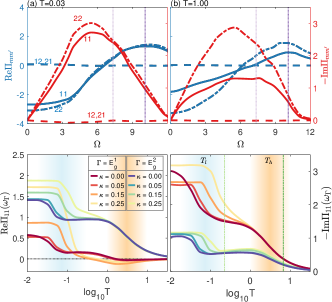
Figure S4: The real and imaginary part of the polarization bubble $\Pi_{mm^{\prime}}$ within a $E_{g}$ channel measured in the units of $\lambda^{2}_{\Gamma}$ ($mm^{\prime}$ components have been indicated in (a)). Panels (a-b): the frequency dependence of $\operatorname{Re}\Pi_{mm^{\prime}}$ and $-\operatorname{Im}\Pi_{mm^{\prime}}$ at different temperatures and $\kappa=0$, corresponding to average flux densities of (a) $n_{\textmd{av}}=0.01$, (b) $n_{\textmd{av}}=0.48$. The two vertical purple lines denote the bare phonon energies $\omega_{E^{1}_{g}}=7.32$ and $\omega_{E^{2}_{g}}=10.1$. Panels (c-d): the temperature dependence of $\operatorname{Re}\Pi_{11}$ and $-\operatorname{Im}\Pi_{11}$ for various $\kappa$ evaluated at $\omega_{E^{1}_{g}}$ and $\omega_{E^{2}_{g}}$ respectively. $T_{l}$ and $T_{h}$ are the two crossover temperatures. The two green vertical dashed lines in (d) indicate $T=5$ K and 150 K. All results are obtained by the strMC method.

We now can perform an explicit calculation of the Raman phonon lineshape. Based on the Dyson equation (C25), the renormalization of the phonon energy and broadening of the peak’s width can be estimated from the polarization bubble $\hat{\Pi}$. When $\kappa=0$, the off-diagonal components of the polarization bubble $\Pi_{mm^{\prime}}$ is negligible as shown in Fig. S4. So the imaginary part of a diagonal entry of the renormalized phonon propagator is given by (we have explicitly moved $\lambda_{\Gamma}$ out of $\Pi$):

$$-\operatorname{Im}D_{mm}(\Omega)=\frac{4\omega^{2}_{\Gamma}\left(\frac{\Omega\delta_{\textmd{ph}}}{\omega_{\Gamma}}-\lambda_{\Gamma}^{2}\operatorname{Im}\Pi_{mm}\right)}{\left(\Omega^{2}-\omega_{\Gamma}^{2}-2\omega_{\Gamma}\lambda_{\Gamma}^{2}\operatorname{Re}\Pi_{mm}\right)^{2}+4\omega_{\Gamma}^{2}\left(\frac{\Omega\delta_{\textmd{ph}}}{\omega_{\Gamma}}-\lambda_{\Gamma}^{2}\operatorname{Im}\Pi_{mm}\right)^{2}},$$ (D1)

where the analytical continuation $i\Omega_{n}\to\Omega+i\delta_{\textmd{ph}}$ has been taken to obtain retarded correlation function $D_{mm}(\Omega)$, and $\delta_{\textmd{ph}}$ is an artificial broadening of the bare phonon peak. As mentioned above, the xx-geometry scattering is controlled by the $mm=11$ component. Then, the half width at half maxima (HWHM) of the phonon peak can be estimated as

$$\gamma_{\textmd{est}} =-\lambda_{\Gamma}^{2}\operatorname{Im}\Pi_{11}+\delta_{\textmd{ph}}.$$ (D2)

Here, note that there is an artificial background contribution to the line width, $\delta_{\textmd{ph}}$, which causes the nonzero line width at $T=\infty$ (numerically at $T=10^{1.5}$). Therefore, both in the main text and here, we offset the computed line width by a background value obtained at the infinite temperature. As shown in Tab. 1, the decrease of peak width $\gamma_{\textmd{MC}}$ (evaluated by the strMC simulations) between 5 K and 150 K is estimated to be $0.055J$. This is comparable to the experimental findings in Ref. Sandilands et al. (2015), that the anomalous peak width $\gamma_{\textmd{exp}}$ displays a decrease of $0.085J$ between 5 K and 150 K . This result indicates that the source of the anomaly comes from the spin-phonon coupling in the vicinity of the Kitaev spin liquid. In the low-temperature region between 0.2 K to 5 K, the estimation of the peak width differs significantly from the strMC result. This is due to the effect of the spin-dependent phonon Raman coupling at low temperatures also causes smaller peak width.

The renormalized peak’s position, $\omega^{\textmd{ren}}_{\Gamma}$, is given by

$$\omega^{\textmd{ren}}_{\Gamma} =\sqrt{\omega_{\Gamma}^{2}+2\omega_{\Gamma}\lambda_{\Gamma}^{2}\operatorname{Re}\Pi_{mm}}\approx\omega_{\Gamma}+\lambda_{\Gamma}^{2}\operatorname{Re}\Pi_{mm}.$$ (D3)

Since $\operatorname{Re}\Pi_{11}>0$, the phonon peak moves towards right. This energy shift decreases with increasing temperature.

$T/K$	0.2	5	150	$\infty$
$\gamma_{\textmd{est}}/J$	0.280	0.150	0.055	0
$\gamma_{\textmd{MC}}/J$	0.225	0.090	0.035	0
$\gamma_{\textmd{exp}}/J$		0.090	0.005

Table 1: The half width at half maxima (HWHM) of the $E_{g}^{2}$ phonon peak at several characteristic temperatures. $\gamma_{\textmd{est}}$ is the HWHM estimated as $\gamma_{\textmd{est}}=-\lambda_{E_{g}^{2}}^{2}\operatorname{Im}\Pi_{11}$, where $\lambda_{E_{g}^{2}}=0.52$ (in units of $J$). $\gamma_{\textmd{MC}}$ is HWHM of $E_{g}^{2}$ phonon obtained from Eq. (C26), evaluated with the strMC simulations on a lattice of $N_{1}=N_{2}=25$ as shown in Fig. 2(b) in the main text. Note that $\gamma_{\textmd{MC}}$ here has been offset by a background line width obtained at $T=\infty$, which mainly comes from the artificial broadening $\delta_{\textmd{ph}}$. $\gamma_{\textmd{exp}}$ is the experimentally measured HWHM, which is the anomalous deviation from the anharmonic behaviour. It is obtained from Ref. Sandilands et al. (2015), and $\gamma_{\textmd{exp}}=\Delta\Gamma/2$ in the notations therein. The two temperatures $5K$ and $150K$ are marked as green dot-dashed lines in Fig. 2(b) in the main text.

Appendix E E. The details of the model fitting

In this section, we describe the details of fitting the experimental Raman spectrum and clarify the uniqueness of the best-fit model parameters $\{\omega_{\Gamma},\lambda_{\Gamma},\nu,\mu_{\Gamma}\}$ up to an overall scaling. First we note that the overall magnitude of Raman spectrum is free to rescale. This degree of freedom is reflected in a simultaneous scaling of the couplings $\{\nu,\mu_{\Gamma}\}$. If they are magnified or reduced uniformly by the same factor, then the resultant calculated spectrum will retain its shape with only an overall scale difference. This can be clearly seen from Eq. (C26) and Feynman diagrams presented in Fig. S3. Thus, we can set $\mu_{E_{g}^{2}}=1$ to fix the overall scale, and get $\mu_{E_{g}^{1}}=0.36\mu_{E_{g}^{2}}$ and $\nu=-0.63\mu_{E_{g}^{2}}$. After getting rid of the overall scaling factor, the model parameters are uniquely decided by the process of fitting the computed Raman intensity to the experimental Raman curve. In this process, $\nu$ controls the overall intensity of the magnetic continuum which is contributed from both $I_{\textmd{em-s}}$ and the spin-dependent phonons Raman couplings, and it also affects the Fano asymmetry of both phonon peaks. $\lambda_{\Gamma}$ controls the phonon peak widths as well as the Fano asymmetry of respective peaks. $\mu_{\Gamma}$ controls the phonon peak heights. $\omega_{\Gamma}$ controls the peak positions. Therefore, each parameter has its unique effect, and changing one of these parameters will not be completely compensated by tuning the others. This guarantees that the optimal set of the model parameters is unique.

Appendix F F. Absence of the Fano lineshape in the phonon Raman response with perpendicular polarization.

In this section, we apply our theory to analyze the polarization-resolved Raman experiment in $\alpha$-RuCl₃ reported in Ref. Mai et al. (2019). This work explores the Raman spectroscopy of the out-of-plane polarizations, and concludes that the spin-related effects, namely the magnetic continuum and Fano lineshape asymmetry, disappear when the photon polarization is perpendicular to the honeycomb plane of Ru³⁺ ions, suggesting that these effects are both of the same two-dimensional origin.

To explore the polarization dependence of the Raman spectroscopy, Eq. (C26) needs to be explicitly evaluated. Following the same set up in Ref. Li et al. (2019), for polarization within the $a$-$c$ plane, we denote the angle between $E$ and $a$ axis as $\phi$. Consider parallel scattering geometry, $E^{\mu}_{in}=E^{\mu}_{out}=[\cos\phi,0,\sin\phi]$. Then the Raman intensity is proportional to

$$\cos^{4}\phi\,\mathcal{I}^{xx}+\sin^{4}\phi\,\mathcal{I}^{zz}+\cos^{2}\phi\sin^{2}\phi\,\mathcal{I}^{xz}+\sin^{2}\phi\cos^{2}\phi\,\mathcal{I}^{zx},$$ (F1)

where $\mathcal{I}^{\mu\mu^{\prime}}$ is defined in Eq. (C26). We focus on the perpendicular polarization $\phi=\pi/2$ so only $\mathcal{I}^{zz}$ is considered. First we analyze the phonon peak in the Raman spectrum, which is contributed from the phonon Raman tensor $R_{\Gamma m}^{\mu\mu^{\prime}}$. As shown in Eq. (B10), $R_{\Gamma m}^{zz}=0$ for $D_{3d}$ group, which indicates that the response in the $zz$ polarization would be identically zero. But if the symmetry is broken to $C_{2h}$, as shown in Ref. Li et al. (2019), the non-zero $R_{\Gamma m}^{zz}$ is allowed so the phonon peak persists at $\phi=0$ there. Therefore, the nonzero peak in the Raman spectrum at perpendicular polarization observed in Ref. Mai et al. (2019) must result from the symmetry breaking from $D_{3d}$ to $C_{2h}$. This symmetry breaking is introduced from the distortion of the honeycomb lattice due to the weak interlayer interaction Mai et al. (2019).