Modulated phases in a spin model with Dzyaloshinskii-Moriya interactions

Abstract

We analyze the phase diagram of an elementary statistical lattice model of classical, discrete, spin variables, with nearest-neighbor ferromagnetic isotropic interactions in competition with chiral interactions along an axis. At the mean-field level, we show the existence of paramagnetic lines of transition to a region of modulated (helimagnetic) structures. We then turn to the analysis of the analogous problem on a Cayley tree. Taking into account the simplicity introduced by the infinite-coordination limit of the tree, we explore several details of the phase diagrams in terms of temperature and a parameter of competition. In particular, we characterize sequences of modulated (helical) structures associated with devil’s staircases of a fractal character.

Keywords: helimagnetism; Dzyaloshinkii-Moriya interactions; competing interactions

1 Introduction

Competing interactions are known to lead to very rich phase diagrams, with critical and multicritical points and sequences of spatially modulated structures [1][2]. The ANNNI model, which stands for axial-next-nearest neighbor Ising model, is perhaps the best investigated statistical lattice model with competing interactions [3][4][5]. In the standard ANNNI model, there are ferrromagnetic interactions between pairs of nearest-neighbor Ising spin variables on the sites of a cubic lattice, with the addition of competing antiferromagnetic interactions between second-neighbor spin pairs along an axial direction. In terms of temperature and a parameter to gauge the competition, the ANNNI model exhibits perhaps the richest phase diagram of the literature, with a wealth of modulated phases and the onset of fractal structures, which have been called devil’s staircases [6][7].

In the present work we were motivated by recent interest in different forms of helimagnetism [8][9], which can be explained in terms of a chiral mechanism proposed by Dzyaloshinskii and Moriya (DM) a long time ago [10]. According to this DM mechanism, interactions are restricted to first neighbors, but with vector spin variables on each lattice site. Modulation effects come from the competition between the usual Heisenberg exchange, of scalar nature, and an additional exchange associated with the vector products of the DM interactions. Different formulations of spin models including competing exchange and DM interactions have indeed been used to account for the monoaxial helical patterns of magnetic compounds [11][12]. We were also motivated by early work for special clock models with chiral interactions, which have been investigated by different techniques [13][14][15]. In contrast to the ANNNI model, elementary lattice model systems associated with the DM mechanism have not been subjected to more detailed statistical mechanics calculations. We then believe that there is still room to analyze some simple and schematic version of these spin models with DM interactions, and to show that they are capable of displaying a phase diagram with many sequences of modulated structures.

We consider a ferromagnetic version of a classical Heisenberg spin model with DM interactions, in zero external field, and restrict the competition to a single lattice axis. The spin Hamiltonian of this simple monoaxial lattice system is written as

$$\mathcal{H}_{DM}=-J_{0}\sum_{\left(\overrightarrow{r},\overrightarrow{r}^{\prime}\right)}^{\left(x,y\right)}\overrightarrow{S}_{\overrightarrow{r}}\cdot\overrightarrow{S}_{\overrightarrow{r}^{\prime}}-J\sum_{\left(\overrightarrow{r},\overrightarrow{r}^{\prime}\right)}^{\left(z\right)}S_{\overrightarrow{r}}^{z}\,S_{\overrightarrow{r}^{\prime}}^{z}-D\sum_{\left(\overrightarrow{r},\overrightarrow{r}^{\prime}\right)}^{\left(z\right)}\left(\overrightarrow{S}_{\overrightarrow{r}}\times\overrightarrow{S}_{\overrightarrow{r}^{\prime}}\right)\cdot\widehat{z},$$ (1)

where $\overrightarrow{S}_{\overrightarrow{r}}$ is a vector spin on site $\overrightarrow{r}$ of a simple cubic crystal lattice, we assume positive exchange parameters, $J_{0}$, $J>0$, the first sum is over nearest-neighbor sites on the $x-y$ planes, and the second and third sums are over nearest-neighbor sites along the $z$ direction. The last term in this spin Hamiltonian provides the competition with the usual exchange term, which is the essential ingredient to mimic a monoaxial DM model system.

We now make another simplifying assumption. Instead of considering continuous variables, we assume discrete vector spin variables, with just six possibilities, along the directions of the Cartesian axes. We then write the six spin components,

$$\overrightarrow{S}_{\overrightarrow{r}}=\begin{pmatrix}1\\ 0\\ 0\end{pmatrix},\,\begin{pmatrix}0\\ 1\\ 0\end{pmatrix},\,\begin{pmatrix}0\\ 0\\ 1\end{pmatrix},\,\begin{pmatrix}-1\\ 0\\ 0\end{pmatrix},\,\begin{pmatrix}0\\ -1\\ 0\end{pmatrix},\,\begin{pmatrix}0\\ 0\\ -1\end{pmatrix}.$$ (2)

Although this is a drastic simplification of the original spin model system, it keeps the essential features of the DM interactions. This formulation, however, is still not amenable to exact calculations. We then resort to well-known mean-field approximate schemes, and analyze the main features of the phase diagrams in terms of temperature and a parameter that gauges the competition.

In Section 2, we formulate a solution of this problem on the basis of a layer-by-layer mean-field calculation, which has been successfully used to investigate the phase diagram of the ANNNI model [16]. Although it is simple to formulate and provides very sensible results, this mean-field calculation demands a considerable numerical effort to unveil the fine details of the phase diagram. We then restrict the analysis to the overall aspects of the phase diagrams. In particular, we locate the paramagnetic transition lines, which already indicate the presence of modulated structures.

In Section 3, we consider an analog of this model system on a Cayley tree. We formulate the statistical problem as a non linear discrete map along the generations of the tree. Attractors of this map, in the deep interior of the tree, are known to correspond to physically realistic solutions, which come from a standard pair approximation for the analogous model system on a Bravais lattice. In the limit of infinite coordination of the tree, the problem becomes considerably simpler, with solutions that should be close to the usual mean-field results. According to earlier calculation for the analog of the ANNNI model on a Cayley tree [17], we take advantage of this infinite-coordination limit to analyze a number of fine details of the phase diagram, including the onset of sequences of modulated structures and the existence of devil’s staircases of a fractal character.

2 Layer-by-layer mean-field calculation

We consider a cubic lattice of $N^{3}$ sites, and split the Hamiltonian (1) into two terms,

$$\mathcal{H}=\mathcal{H}_{1}+\mathcal{H}_{2},$$ (3)

where the first term includes the nearest-neighbor pair interactions on the $x-y$ planes of the lattice,

$$\mathcal{H}_{1}=-J_{0}\sum_{z=1}^{N}\sum_{\left(x,y;\,\,x^{\prime}y^{\prime}\right)}\left[S_{x,y,z}^{x}S_{x^{\prime},y\prime,z}^{x}+S_{x,y,z}^{y}S_{x^{\prime},y\prime,z}^{y}+S_{x,y,z}^{z}S_{x^{\prime},y\prime,z}^{z}\right],$$ (4)

and the second term refers to the interactions along the axial $z$ direction,

$$\mathcal{H}_{2}=-J\sum_{x,y}\sum_{z=1}^{N}\left[S_{x,y,z}^{x}S_{x,y,z+1}^{x}+S_{x,y,z}^{y}S_{x,y,z+1}^{y}+S_{x,y,z}^{z}S_{x,y,z+1}^{z}\right]-$$

$$-D\sum_{x,y}\sum_{z=1}^{N}\left[S_{x,y,z}^{x}S_{x,y,z+1}^{y}-S_{x,y,z}^{y}S_{x,y,z+1}^{x}\right].$$ (5)

We now use the Bogoliubov inequality,

$$G\left(\mathcal{H}\right)\leq G_{0}\left(\mathcal{H}_{0}\right)+\left\langle\mathcal{H}-\mathcal{H}_{0}\right\rangle_{0}=\Phi,$$ (6)

where $G\left(\mathcal{H}\right)$ is the free energy associated with $\mathcal{H}$, $G_{0}\left(\mathcal{H}_{0}\right)$ is the free energy associated with a trial Hamiltonian $\mathcal{H}_{0}$, and $\left\langle...\right\rangle_{0}$ is an expected value in a canonical ensemble defined by the trial Hamiltonian. The mean-field approximation consists in assuming that the free energy of this system comes from the minimization of the upper bound $\Phi$ with respect to the parameters of the trial Hamiltonian.

The simplest form of a trial Hamiltonian, which still preserves the possibility of modulated structures along the $z$ axis, is given by

$$\mathcal{H}_{0}=-\sum_{x,y}\sum_{z}\overrightarrow{\eta}_{z}\cdot\overrightarrow{S}_{x,y,z}=-\sum_{x,y}\sum_{z}\left[\eta_{z}^{x}S_{x,y,z}^{x}+\eta_{z}^{y}S_{x,y,z}^{y}+\eta_{z}^{z}S_{x,y,z}^{z}\right],$$ (7)

where $\overrightarrow{\eta}_{z}=\left(\eta_{z}^{x},\eta_{z}^{y},\eta_{z}^{z}\right)$ is a three-component trial field. We then have

$$G_{0}=-\frac{N^{2}}{\beta}\sum_{z}\ln\left[2\cosh\left(\beta\eta_{z}^{x}\right)+2\cosh\left(\beta\eta_{z}^{y}\right)+2\cosh\left(\beta\eta_{z}^{z}\right)\right]$$ (8)

and

$$\frac{1}{N^{2}}\left\langle\mathcal{H}-\mathcal{H}_{0}\right\rangle_{0}=-2J_{0}\sum_{z}\left[\left(m_{z}^{x}\right)^{2}+\left(m_{z}^{y}\right)^{2}+\left(m_{z}^{z}\right)^{2}\right]-$$

$$-J\sum_{z}\left[m_{z}^{x}m_{z+1}^{x}+m_{z}^{y}m_{z+1}^{y}+m_{z}^{z}m_{z+1}^{z}\right]-$$

$$-D\sum_{z}\left[m_{z}^{x}m_{z+1}^{y}-m_{z}^{y}m_{z+1}^{x}\right]+\sum_{z}\left[\eta_{z}^{x}m_{z}^{x}+\eta_{z}^{y}m_{z}^{y}+\eta_{z}^{z}m_{z}^{z}\right],$$ (9)

in which we have introduced the definitions

$$m_{z}^{\nu}=\frac{\sinh\left(\beta\eta_{z}^{\nu}\right)}{\cosh\left(\beta\eta_{z}^{x}\right)+\cosh\left(\beta\eta_{z}^{y}\right)+\cosh\left(\beta\eta_{z}^{z}\right)},$$ (10)

where $\nu=x$, $y$, $z$, and $\beta=1/\left(k_{B}T\right)$ is the inverse of temperature.

The minimization of $\Phi$ with respect to the trial fields $\left\{\overrightarrow{\eta}_{z}\right\}$ leads to the equations

$$\eta_{z}^{x}=4J_{0}m_{z}^{x}+J\left(m_{z-1}^{x}+m_{z+1}^{x}\right)+D\left(m_{z-1}^{y}-m_{z+1}^{y}\right),$$ (11)

$$\eta_{z}^{y}=4J_{0}m_{z}^{y}+J\left(m_{z-1}^{y}+m_{z+1}^{y}\right)-D\left(m_{z-1}^{x}-m_{z+1}^{x}\right),$$ (12)

and

$$\eta_{z}^{z}=4J_{0}m_{z}^{z}+J\left(m_{z-1}^{z}+m_{z+1}^{z}\right).$$ (13)

We now insert these expressions for the trial fields into the definitions of the local magnetizations, given by (10), and write an infinite system of nonlinear coupled mean-field equations of state for the local magnetizations.

As in the mean-field calculations for the ANNNI model [16], given the temperature and the parameters of the system, the problem consists in finding a multiple set of numerical solutions, and choosing the solution that minimizes the free energy. Except in the immediate neighborhood of a critical line, this search for the physically acceptable solutions becomes a purely numerical problem. Usually, we find a numerical solution with the assumption of a periodicity of $L$ lattice spacings along the $z$ direction, and take note of the associated value of the free energy. We then repeat this procedure for a sequence of values of $L$. Physically acceptable solutions are shown to minimize the free energy with respect to the length $L$. Instead of carrying out this cumbersome numerical calculation, we now turn to an expansion of the free energy.

It is easy to write the mean-field free energy as a power series in the spin magnetizations, and make contact with a Landau-Ginzburg expansion. Keeping terms up to order $4$, we have

$$\frac{1}{N^{3}}\Phi=-\frac{1}{\beta}\ln 6+\frac{1}{N}\sum_{z}\left(-2J_{0}+\frac{3}{2\beta}\right)\left[\left(m_{z}^{x}\right)^{2}+\left(m_{z}^{y}\right)^{2}+\left(m_{z}^{z}\right)^{2}\right]-$$

$$-\frac{J}{N}\sum_{z}\left[m_{z}^{x}m_{z+1}^{x}+m_{z}^{y}m_{z+1}^{y}+m_{z}^{z}m_{z+1}^{z}\right]-\frac{D}{N}\sum_{z}\left[m_{z}^{x}m_{z+1}^{y}-m_{z}^{y}m_{z+1}^{x}\right]+$$

$$+\frac{9}{4\beta N}\sum_{z}\left[\left(m_{z}^{x}\right)^{2}\left(m_{z}^{y}\right)^{2}+\left(m_{z}^{x}\right)^{2}\left(m_{z}^{z}\right)^{2}+\left(m_{z}^{y}\right)^{2}\left(m_{z}^{z}\right)^{2}\right]+...$$ (14)

We then assume periodic boundary conditions, and use a Fourier representation,

$$m_{z}^{\nu}=\frac{1}{\sqrt{N}}\sum_{q}m_{q}^{\nu}\exp\left(iqz\right),$$ (15)

where $\nu=x,y,z$, and the sum is restricted to the first, and symmetric, Brillouin zone. Also, it is convenient to write

$$m_{q}^{\nu}=\frac{1}{\sqrt{2}}(R_{q}^{\nu}+iI_{q}^{\nu}),$$ (16)

with

$$R_{q}^{\nu}=R_{-q}^{\nu},\qquad I_{q}^{\nu}=-I_{-q}^{\nu}.$$ (17)

Keeping terms up to second order, we have

$$\frac{1}{N^{3}}\Phi-\frac{1}{\beta}\ln 6=$$

$$=\frac{1}{2}\sum_{q}\left(\frac{3}{2\beta}-2J_{0}-J\cos q\right)\left[\left(R_{q}^{x}\right)^{2}+\left(I_{q}^{x}\right)^{2}+\left(R_{q}^{y}\right)^{2}+\left(I_{q}^{y}\right)^{2}+\left(R_{q}^{z}\right)^{2}+\left(I_{q}^{z}\right)^{2}\right]-$$

$$-D\sum_{q}\left(\operatorname{sen}q\right)\left[I_{q}^{x}R_{q}^{y}-I_{q}^{y}R_{q}^{x}\right]+\cdot\cdot\cdot,$$ (18)

which is a quadratic form in terms of the real normal modes in Fourier space. Note the symmetry along the $q$ axis. Also, note that the coupling is restricted to the $x-y$ real modes only. It is then convenient to define

$$A=\frac{3}{4\beta}-J_{0}-\frac{1}{2}J\cos q;\qquad B=D\operatorname{sen}q,$$ (19)

and to introduce the simplified notation

$$x_{1}=R_{q}^{x};\quad x_{2}=I_{q}^{x};\quad y_{1}=R_{q}^{y};\quad y_{2}=I_{q}^{y}\quad z_{1}=R_{q}^{z};\quad z_{2}=I_{q}^{z}.$$ (20)

We then have to analyze the quadratic form

$$Q=A\left(x_{1}^{2}+x_{2}^{2}+y_{1}^{2}+y_{2}^{2}+z_{1}^{2}+z_{2}^{2}\right)+B\left(y_{2}x_{1}-x_{2}y_{1}\right)=\left(\overrightarrow{v}\right)^{t}\mathbf{M}\left(\overrightarrow{v}\right),$$ (21)

in which $\overrightarrow{v}$ is a column vector, $\widetilde{\mathbf{v}}=\left(x_{1},x_{2},y_{1},y_{2},z_{1},z_{2}\right)$, and the matrix $\mathbf{M}$ is given by

$$\mathbf{M}=\left(\begin{array}[c]{cccccc}A&0&0&B/2&0&0\\ 0&A&-B/2&0&0&0\\ 0&-B/2&A&0&0&0\\ B/2&0&0&A&0&0\\ 0&0&0&0&A&0\\ 0&0&0&0&0&A\end{array}\right).$$ (22)

This matrix has two trivial real and degenerate eigenvalues,

$$\lambda_{1}=\lambda_{2}=A=\frac{3}{4\beta}-J_{0}-\frac{1}{2}J\cos q.$$ (23)

The remaining eigenvalues are associated with a $4\times 4$ supersymmetric matrix. We then have

$$\lambda_{3,4}=A\pm\frac{1}{2}B=\frac{3}{4\beta}-J_{0}-\frac{1}{2}J\cos q\pm\frac{1}{2}D\sin q.$$ (24)

Taking into account the form of these eigenvalues, it is immediate to obtain an expression for the border of the disordered region,

$$\frac{1}{\beta_{c}}=k_{B}T_{c}=\max\limits_{q}\left[\frac{4}{3}J_{0}+\frac{2}{3}J\,\cos q\pm\frac{2}{3}D\,\sin q\right].$$ (25)

For $D=0$, we recover the (mean-field) critical temperature of a simple ferromagnet,

$$\frac{1}{\beta_{c}^{F}}=k_{B}T_{c}^{F}=\max\limits_{q}\left(\frac{4}{3}J_{0}+\frac{2}{3}J\cos q\right)=\frac{4}{3}J_{0}+\frac{2}{3}J,$$ (26)

For $D\neq 0$, we have

$$\tan q=\pm\frac{D}{J},$$ (27)

which corresponds to propagating waves along the two directions of the $z$ axis, with the critical temperature

$$\frac{1}{\beta_{c}^{M}}=k_{B}T_{c}^{M}=\frac{4}{3}J_{0}+\frac{2}{3}\left(J^{2}+D^{2}\right)^{1/2}.$$ (28)

From equations (26) and (28) we have the paramagnetic transition lines,

$$k_{B}T_{c}^{F}-\frac{4}{3}J_{0}=\frac{2}{3}J\text{ },\qquad k_{B}T_{c}^{M}-\frac{4}{3}J_{0}=\frac{2}{3}\left(J^{2}+D^{2}\right)^{1/2}.$$ (29)

These equations indicate that there is always a transition to a spatially modulated structure, except at a trivial, ferromagnetic, multicritical point, at $D=0$.

3 Analysis of the DM model on a Cayley tree

We now turn to calculations for the analogous DM model on a Cayley tree, which is perhaps the simplest way to unveil the rich structure of the ordered phases. We then consider the monoaxial Hamiltonian,

$$\mathcal{H}=-J\sum_{\left(\overrightarrow{r},\overrightarrow{r}^{\prime}\right)}\overrightarrow{S}_{\overrightarrow{r}}\cdot\overrightarrow{S}_{\overrightarrow{r}^{\prime}}-D\sum_{\left(\overrightarrow{r},\overrightarrow{r}^{\prime}\right)}\left(\overrightarrow{S}_{\overrightarrow{r}}\times\overrightarrow{S}_{\overrightarrow{r}^{\prime}}\right)\cdot\widehat{z},$$ (30)

where $J>0$, and $\overrightarrow{r}$ and $\overrightarrow{r}^{\prime}$ are nearest-neighbor sites along the successive generations of a Cayley tree (and we discard ferromagnetic interactions between sites belonging to the same generation of the tree). Although it is not entirely similar to the previously analyzed mean-field model, the formulation on a Cayley tree is known to lead to essentially the same qualitative results [18]. Also, the problem is written as a nonlinear dissipative discrete map, along the generations of a Cayley tree, which is much easier to analyze than the corresponding area-preserving map associated with the mean-field solutions. Attractors of this dissipative mapping problem are known to mimic the phase structure of the ordered region of the mean-field phase diagrams.

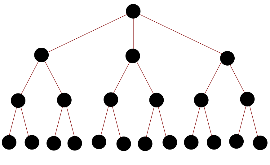
Figure 1: Sketch of three generations of a Cayley tree with coordination three.

In Figure 1, we sketch a Cayley tree of coordination $z=3$ (and ramification $r=z-1=2$). We then consider a tree of arbitrary ramification $r$, and use well-known procedures to write six recursion relations,

$$Z_{1}^{\prime}=\left(e^{\beta J}Z_{1}+e^{\beta D}Z_{2}+Z_{3}+e^{-\beta J}Z_{4}+e^{-\beta D}Z_{5}+Z_{6}\right)^{r},$$ (31)

$$Z_{2}^{\prime}=\left(e^{-\beta D}Z_{1}+e^{\beta J}Z_{2}+Z_{3}+e^{\beta D}Z_{4}+e^{-\beta J}Z_{5}+Z_{6}\right)^{r},$$ (32)

$$Z_{3}^{\prime}=\left(Z_{1}+Z_{2}+e^{\beta J}Z_{3}+Z_{4}+Z_{5}+e^{-\beta J}Z_{6}\right)^{r},$$ (33)

$$Z_{4}^{\prime}=\left(e^{-\beta J}Z_{1}+e^{-\beta D}Z_{2}+Z_{3}+e^{\beta J}Z_{4}+e^{\beta D}Z_{5}+Z_{6}\right)^{r},$$ (34)

$$Z_{5}^{\prime}=\left(e^{\beta D}Z_{1}+e^{-\beta J}Z_{2}+Z_{3}+e^{-\beta D}Z_{4}+e^{\beta J}Z_{5}+Z_{6}\right)^{r},$$ (35)

$$Z_{6}^{\prime}=\left(Z_{1}+Z_{2}+e^{-\beta J}Z_{3}+Z_{4}+Z_{5}+e^{\beta J}Z_{6}\right)^{r},$$ (36)

where $Z_{i}^{\prime}$ is a partial partition function associated with a central site in the spin state $i$, given by equation (2), which is related to the partial partition functions, $Z_{1}$ to $Z_{6}$, associated with the nearest-neighbor sites belonging to the next generation of the tree. The cycle-free structure of the Cayley tree enormously simplifies the form of these recursion relations. It is worth to remark that, for $r=1$, we regain the transfer matrix associated with the solution of the corresponding model on a chain.

Although it is not difficult to analyze these recursion relations, we further simplify the problem, and at the same time emphasize the analogy with the mean-field results, by resorting to the infinite coordination limit of the tree. We then take $r\rightarrow\infty$, and $J$, $D\rightarrow 0$, but keep fixed the products $Jr$ and $Dr$.

In this infinite-coordination limit, the problem is reduced to the analysis of just three recursion relations, which involve the vector components of the average of an “effective magnetization”,

$$m_{x}^{\prime}=\frac{1}{M}\left[\sinh(\beta Jrm_{x}+\beta Drm_{y})\right],$$ (37)

$$m_{y}^{\prime}=\frac{1}{M}\left[\sinh(-\beta Drm_{x}+\beta Jrm_{y})\right],$$ (38)

$$m_{z}^{\prime}=\frac{1}{M}\left[\sinh(\beta Jrm_{z})\right],$$ (39)

with the denominator

$$M=\cosh(\beta Jrm_{x}+\beta Drm_{y})+\cosh(-\beta Drm_{x}+\beta Jrm_{y})+\cosh(\beta Jrm_{z}).$$ (40)

We now use analytical and numerical techniques to analyze the attractors of this map.

3.1 Attractors of the map

There is always a trivial solution, $m_{x}^{\ast}=m_{y}^{\ast}=m_{z}^{\ast}=0$ of equations (37)-(39). The linearization about this trivial fixed point leads to the matrix equation

$$\overrightarrow{m}^{\prime}=\mathbf{M}\,\overrightarrow{m},$$ (41)

where

$$M=\frac{1}{3}\begin{pmatrix}\beta Jr&\beta Dr&0\\ -\beta Dr&\beta Jr&0\\ 0&0&\beta Jr\end{pmatrix}.$$ (42)

Therefore, we have the eigenvalues

$$\lambda_{1}=\frac{1}{3}\beta Jr,$$ (43)

$$\lambda_{2}=\frac{1}{3}(\beta Jr+i\beta Dr),$$ (44)

and

$$\lambda_{3}=\frac{1}{3}(\beta Jr-i\beta Dr).$$ (45)

The conditions of linear stability of this trivial (disordered) fixed point are given by

$$T>\frac{1}{3},$$ (46)

and

$$T>\frac{\left(1+p^{2}\right)^{1/2}}{3},$$ (47)

where we have introduced a simplified notation, $T=1/\left(\beta Jr\right)$ and $p=D/J$. We then have a similar picture as in the previous mean-field calculation. There is always a paramagnetic transition, which is associated with the complex eigenvalues of the trivial fixed point, except at $p=0$, which leads to a simple ferromagnetic transition.

In order to go beyond the linear analysis, and investigate the stability of additional attractors, we have to resort to numerical calculations. We then characterized two types of behavior: (i) in one of these possibilities, the magnetization settles in a specific value (one of the components settles in the value $1$, and the other components vanish); (ii) the second possibility is a cyclic pattern in the representation of $m_{x}$ versus $m_{y}$, as we indicate in Figure 2 (the component $m_{z}$ of the magnetization flows to a fixed value, as in the first case). The first possibility leads to a quite trivial ordered structure. The second possibility, however, leads to a spatially modulated structure.

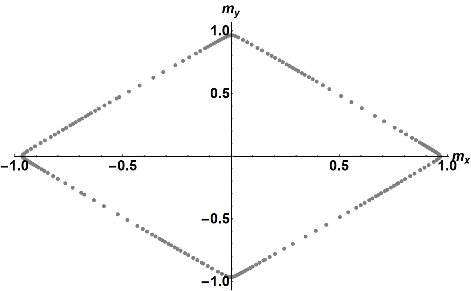
Figure 2: Graph of $200$ iterations of $m_{y}$ versus $m_{x}$, for $T=0.2$ and $p=0.9$. We assume the initial values $m_{x}=m_{y}=m_{z}=1$, and discard the initial $10000$ iterations. This modulated structure is characterized by the wave number of the main harmonic component, $q/2\pi=0.13$ (assuming a unit lattice paramater).

We have used this numerical procedure to sketch the phase diagram of Figure 3. Attractors of the map correspond to disordered (D), ferromagnetically ordered (O), and spatially modulated (M) structures. In general, given the values of reduced temperature $T$ and the parameter $p=D/J$, we choose arbitrary initial conditions ($0<m_{x},m_{y},m_{z}<1$) and iterate equations (37) to (39) about $10^{4}$ times. Final values of the magnetizations $m_{x}$ and $m_{y}$ are determined with a precision of about $10^{-5}$ (the component $m_{z}$ does not display any modulation).

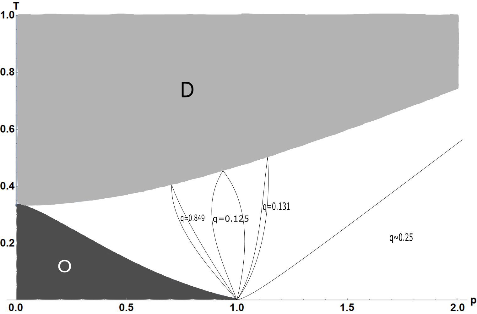
Figure 3: Phase diagram in terms of temperature ($T$) and the parameter of chirality ($p=D/J$). We indicate disordered (D), ferromagnetically ordered (O) and some spatially modulated phases (in the white region). We use the dimensionless wave number, $q/2\pi$, which is written in terms of $2\pi$, to indicate some of the main modulated phases. In the groud state, for $p>1$, we have $q/2\pi=0.25$.

4 The devil’s staircases

The devil’s staircase is a fractal structure that has been associated with the sequences of modulated structures in the ordered region of the phase diagrams of lattice statistical models, in particular the ANNNI model, with competing interactions. We show that the same kind of behavior comes from the analysis of the iterates of equations (37) to (39).

Given the parameters $T$ and $p$, we plot a graph of $m_{y}$ versus $m_{x}$, as shown in Figure 2, and note that the attractor is a periodic function, which gives rise to the definition of a period $q$ in units of $2\pi$. In a more precise calculation, we perform a Fourier analysis of the attractor and find the main Fourier component, which sets the period $q$. In Figure 4 we plot the wave number $q$ versus the chiral parameter $p$, for a fixed value of temperature, $T=0.2$, which already displays the characteristic shape of a devil’s staircase.

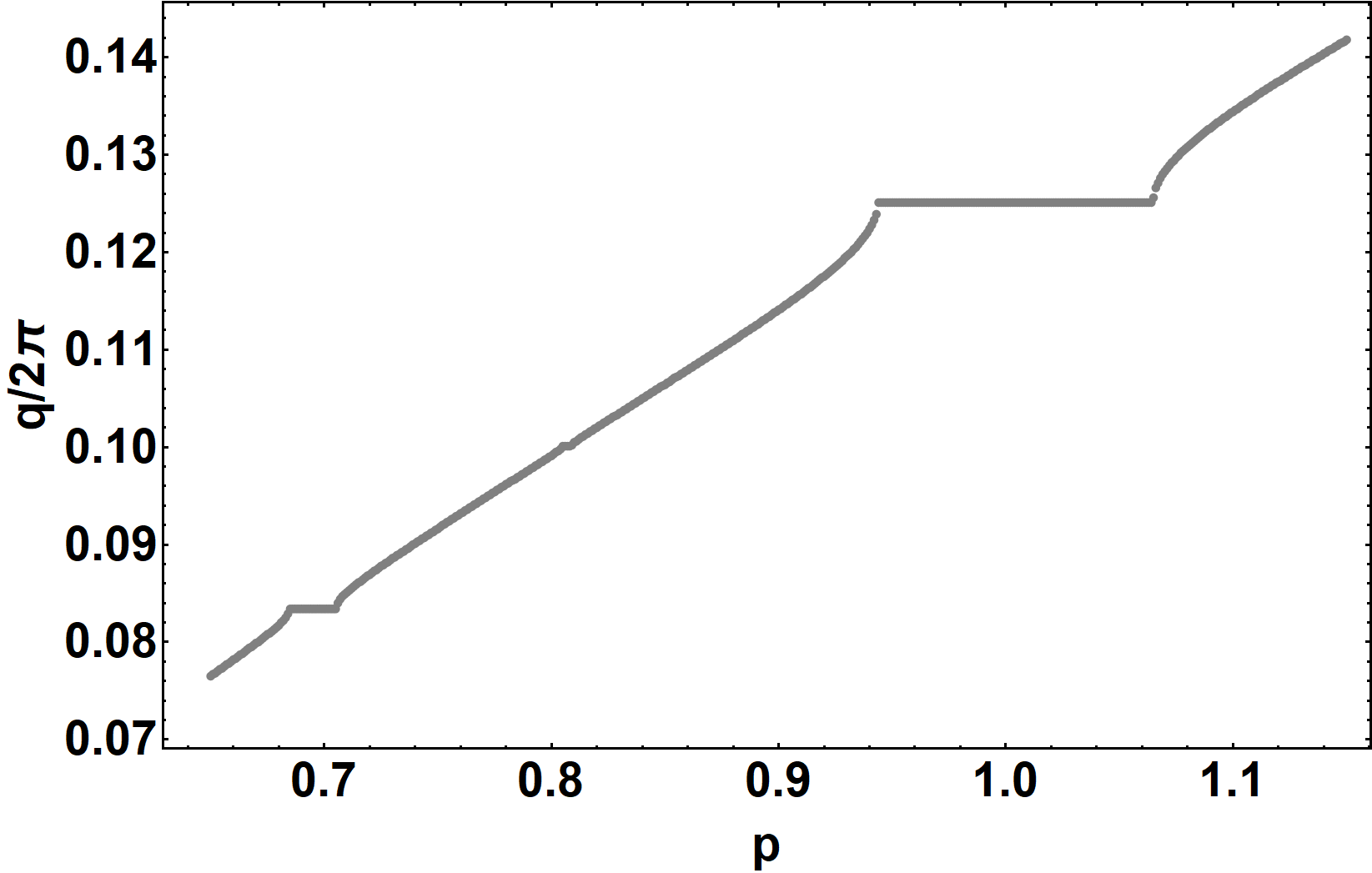
Figure 4: Sketch of a devil’s staircase at $T=0.2$.

We now turn to the calculation of the Hausdorff dimension associated with these plots of $q$ versus $p$, which leads to the characterization of the fractal nature of the devil’s staircase. According to a box-counting algorithm [7], we choose a value $\epsilon>0$, and then calculate the sum of the step sizes, along the $p$ axis, of all steps with width (size along the $p$ axis) larger than than $\epsilon$. We then subtract the total width of the $p$ interval and obtain the function $X(\epsilon)$. The slope of a plot of $\log(X(\epsilon)/\epsilon)$ versus $\log(1/\epsilon)$, in the limit of small $\epsilon$, leads to an estimate of the Hausdorff dimension $D_{H}$ of the staircase. In the modulated region, we found several examples of plots of $q$ versus $p$, at fixed temperature, with $D_{H}<1$, which characterizes a fractal object. Also, we observed that $D_{H}$ increases with temperature, which indicates a route to an incommensurate structure. In figure 5, we show one of these plots of the Hausdorff dimension versus normalized temperature.

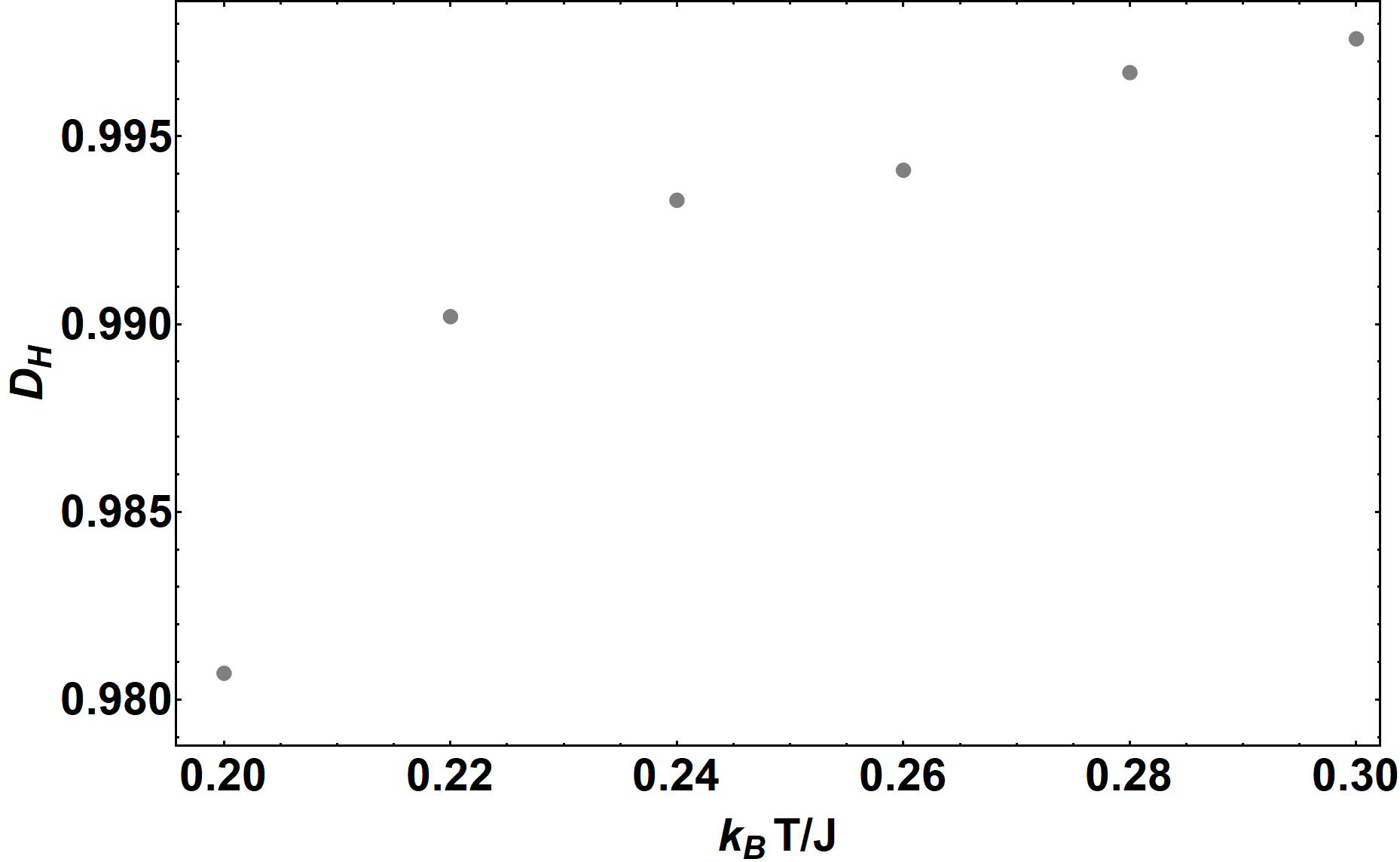
Figure 5: Plot of the Hausdorff dimension as a function of normalized temperature $T$, calculated in the interval $0.65<p<1.15.$

The increase of the Hausdorff dimension $D_{H}$ with $T$ ($D_{H}\rightarrow 1$ as $T\rightarrow T_{c}$) indicates the typical route to an incommensurate structure.

5 Conclusions

We used mean-field approximations to analyze the phase diagram of an elementary system of discrete classical spin variables on a crystal lattice, with ferromagnetic nearest-neighbor exchange interactions and the addition of competing chiral interactions along an axis. This is perhaps the simplest three-dimensional lattice system with the inclusion of Dzyaloshinskii-Moriya interactions. We show that this monoaxial system displays the characteristic modulated phases of helimagnetic compounds. Besides writing the equations of a conventional mean-field layer-by-layer calculation, which already indicates the existence of transitions to modulated structures, we performed some detailed calculations for the analogous model on a Cayley tree, in the limit of infinite coordination. Calculations on the tree confirm the general features of the mean-field results, and provide a simpler way to check fine details of the phase diagrams, in terms of temperature and a parameter of chirality. In particular, we show the existence of many sequences of modulated structures. Also, we confirm the existence of devil’s staircases, which are associated with a non-integer Hausdorff dimension.

Acknowledgment

We acknowledge many fruitful discussions with Doctor Eduardo S. Nascimento. Also, we acknowledge the financial support of the Brazilian agencies CNPq and CAPES.

References

- [1] M. Seul and D. Andelman, Science, 267, 476–483 (1995).
- [2] D. Andelman and R. E. Rosensweig, J. Phys. Chem. B 113, 3785–3798 (2009).
- [3] P. Bak, Repts. Progr. Phys. 45, 587, 1982.
- [4] W. Selke, Phys. Rep. 170, 213, 1988.
- [5] J. Yeomans, Sol. State Phys. 41, 151, 1988.
- [6] W. Selke, “Spatially modulated structures in systems with competing interactions” in Phase Transitions and Critical Phenomena, Vol. 15, p.1-72, ed. by C. Domb and J.L. Lebowitz (Academic Press, 1992).
- [7] E. S. Nascimento, J. P. de Lima and S. R. Salinas, Physica A 409, 78–86 (2014).
- [8] U. K. Rossler, A. N. Leonov, A. N. Bogdanov, J. Phys. Conf. Ser. 200, 022029 (2010).
- [9] N. Nagaosa, Y. Tokura, Nature Nanotechnology 8, 899 (2010).
- [10] Yu. A. Izyumov, Sov. Phys. Usp. 27, 845, 1984.
- [11] J. Kishine, K. Inoue, Y. Yoshida, Progr. Theor. Phys. Suppl. 159, 82, 2005.
- [12] M. Shinozaki, S. Hoshino, Y. Masaki, J. Kishine, Y. Kato, J. Phys. Soc. Jpn. 85, 074710, 2016; T. Toretsume, T. Kikuchi, R. Anita, J. Phys. Soc. Jpn. 87, 041011, 2018.
- [13] D. A. Huse, Phys. Rev. B24, 5180, 1981.
- [14] S. Ostlund, Phys. Rev. B24, 398, 1981.
- [15] H. C. Öttinger, J. Phys. C16, L257, 1983; J. Phys. C16, L597, 1983.
- [16] C. S. O. Yokoi, M. D. Coutinho-Filho, S. R. Salinas, Phys. Rev. B24, 4047, 1981.
- [17] C. S. O. Yokoi, M. J. de Oliveira, S. R. Salinas, Phys. Rev. Lett. 54, 163, 1985.
- [18] M. J. de Oliveira and S. R. Salinas, J. Phys. A18, L1157, 1985.