ImageBART: Bidirectional Context with Multinomial Diffusion for Autoregressive Image Synthesis
Abstract
Autoregressive models and their sequential factorization of the data likelihood have recently demonstrated great potential for image representation and synthesis. Nevertheless, they incorporate image context in a linear 1D order by attending only to previously synthesized image patches above or to the left. Not only is this unidirectional, sequential bias of attention unnatural for images as it disregards large parts of a scene until synthesis is almost complete. It also processes the entire image on a single scale, thus ignoring more global contextual information up to the gist of the entire scene. As a remedy we incorporate a coarse-to-fine hierarchy of context by combining the autoregressive formulation with a multinomial diffusion process: Whereas a multistage diffusion process successively removes information to coarsen an image, we train a (short) Markov chain to invert this process. In each stage, the resulting autoregressive ImageBART model progressively incorporates context from previous stages in a coarse-to-fine manner. Experiments show greatly improved image modification capabilities over autoregressive models while also providing high-fidelity image generation, both of which are enabled through efficient training in a compressed latent space. Specifically, our approach can take unrestricted, user-provided masks into account to perform local image editing. Thus, in contrast to pure autoregressive models, it can solve free-form image inpainting and, in the case of conditional models, local, text-guided image modification without requiring mask-specific training.
1 Introduction
Spurred by the increasingly popular attention mechanism, a remarkably simple principle has driven progress in deep generative modeling over the past few years: Factorizing the likelihood of the data in an autoregressive (AR) fashion
| (1) |
and subsequently learning the conditional transition probabilities with an expressive neural network such as a transformer [72]. The success of this approach is evident in domains as diverse as language modeling [5], music generation [14], neural machine translation [43, 73], and (conditional) image synthesis [51, 6]. However, especially for the latter task of image synthesis, which is also the focus of this work, the high dimensionality and redundancy present in the data challenges the direct applicability of this approach.
Missing Bidirectional Context Autoregressive models which represent images as a sequence from the top-left to the bottom-right have demonstrated impressive performance in sampling novel images and completing the lower half of a given image [6, 18]. However, the unidirectional, fixed ordering of sequence elements not only imposes a perceptually unnatural bias to attention in images by only considering context information from left or above. It also limits practical applicability to image modification: Imagine that you only have the lower half of an image and are looking for a completion of the upper half then these models fail at this minor variation of the completion task. The importance of contextual information from both directions [33] has also been recognized in the context of language modeling [12, 42]. However, simply allowing bidirectional context as in [12] does not provide a valid factorization of the density function for a generative model. Furthermore, the sequential sampling strategy introduces a gap between training and inference, as training relies on so-called teacher-forcing [3] (where ground truth is provided for each step) and inference is performed on previously sampled tokens. This exposure bias can introduce significant accumulations of errors during the generation process, affecting sample quality and coherence [54].
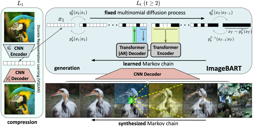
Global Context & Control via Multinomial Diffusion We propose a coarse-to-fine approach that addresses the unidirectional bias of generative autoregressive models and their exposure bias as well as the lacking global context. We formulate learning the data density as a hierarchical problem. A coarser stage provides compressed contextual side information about the entire image for the autoregressive process on the next finer stage. We utilize a diffusion process to gradually eliminate information and compress the data, yielding a hierarchy of increasingly abstract and compact representations. The first scale of this approach is a discrete representation learning task (cf. [71, 55, 14, 18, 75, 53]). Subsequently, we further compress this learned representation via a fixed, multinomial diffusion process [62, 27]. We then invert this process by training a Markov chain to recover the data from this hierarchy. Each Markovian transition is modeled autoregressively but it simultaneously attends to the preceding state in the hierarchy, which provides crucial global context to each individual autoregressive step. As each of this steps can also be interpreted as learning a denoising cloze task [42], where missing tokens at the next finer stage are “refilled” with a bidirectional encoder and an autoregressive decoder, we dub our approach ImageBART.
Contributions of our work Our approach tackles high-fidelity image synthesis with autoregressive models by learning to invert a fixed multinomial diffusion process in a discrete space of compact image representations to successively introduce context. This reduces both the often encountered exposure bias of AR models and also enables locally controlled, user-interactive image editing. Additionally, our model effectively handles a variety of conditional synthesis tasks and our introduced hierarchy corresponds to a successively compressed image representation. We observe that our model sample visually plausible images while still enabling a trade-off between reconstruction capability and compression rate.
2 Related Work
Latent Variable Models Among likelihood-based approaches, latent variable models represent a data distribution with the help of unobserved latent variables. For example, Variational Autoencoders (VAEs) [35, 56] encode data points into a lower dimensional latent variable with a factorized distribution. This makes them easy to sample, interpolate [41, 34] and modify [74]. In a conditional setting [36], latent variables which are independent from the conditioning lead to disentangled representations [28, 66, 45, 57]. A hierarchy of latent variables [63] gives mutli-scale representations of the data. Unfortunately, even the deepest instantiations of these models [44, 68, 8] lack in sample quality compared to other generative models and are oftentimes restricted to highly regular datasets.
Autoregressive Models AR models represent a distribution as a product of conditional, learnable factors via the chain rule of probability densities. While this makes them powerful models for density estimation [67, 21], their samples often lack global consistency. Especially on image data modeled with convolutional architectures [70, 59], this has been attributed to a locality bias of convolutional neural networks (CNNs) which biases the model towards strong local correlations between neighboring pixels at the expense of a proper modeling of coherence [37, 19]. This leads to samples resembling texture patterns without discernible global structure. Attempts to fix this properties by including explicit latent variables [24, 7, 19] have not been overly successful, mainly due the expressiveness of AR models, providing little incentive for learning additional latent variables.
Generative Models on Improved Representations Another successful line of work first learn an improved image representation and subsequently learn a generative model for this representation [71, 10]. Most works [55, 18, 53] learn a discrete representation which is subsequently modeled autoregressively but approaches using continuous representations in combination with VAEs [10], or normalizing flows [1, 57, 17], exist too. Learning a compact representation enables the use of transformers for autoregressive modeling [6], which avoids the locality bias of CNNs, can be used for the synthesis of complex scenes conditioned on text as in DALL-E [53], and, when combined with adversarial learning [22], enables sampling of coherent high-resolution images [18]. However, AR modeling of a learned representation still limits applications compared to latent variable models. Their samples can still exert artifacts resulting from a sequential modeling of components, and, since these models are always trained by “teacher-forcing”, they are susceptible to an exposure bias [3, 54, 23, 60, 40].
Diffusion Probabilistic Models Diffusion probabilistic models revert a fixed, diffusion process with a learned Markov Chain [62]. Being directly applied in pixel space, however, downstream analysis reveals that these models tend to optimize subtle details of the modeled data, which have little contribution to the sample quality [26, 13], particularly hindering applications on high-resolution and -complexity datasets. By using a multinomial diffusion process [27] (recently generalized by [2]) on a compressed, discrete representation of images, we circumvent these issues. Diffusion probabilistic models require a very large number of diffusion steps in order to model the reverse process with a model distribution that factorizes over components. Because our approach uses autoregressively factorized models for the reverse process, we can reduce the required number of steps and obtain significant improvements in sampling speed and the ability to model complex datasets.
3 Method
3.1 Hierarchical Generative Models
To tackle the difficult problem of modeling a highly complex distribution of high-dimensional images , we (i) introduce bidirectional context into an otherwise unidirectional autoregressive factorization of as in Eq. (1) and (ii) reduce the difficulty of the learning problem with a hierarchical approach. To do so, we learn a sequence of distributions , such that each distribution models a slightly more complex distribution with the help of a slightly simpler distribution one level above. This introduces a coarse-to-fine hierarchy of image representations , such that an is modeled conditioned on , i.e. and defines a reverse Markov Chain for as . Since our goal is to approximate the original distribution with , we introduce a forward Markov Chain, , to obtain a tractable upper bound on the Kullback-Leibler (KL) divergence between and , , using the evidence lower bound (ELBO). With , we obtain
| (2) |
We use to learn a compressed and discrete representation of images, such that subsequent stages of the hierarchy do not need to model redundant information (Sec. 3.2). With we learn a model that can rely on global context from a coarser representation to model the representation (Sec. 3.3). See Fig. 1 for an overview of the proposed model.
3.2 Learning a compact, discrete representation for images
Since the first stage of the hierarchical process is the one that operates directly on the data, we assign it a separate role. To avoid that the optimization of () in Eq. (2) unnecessarily wastes capacity on redundant details in the input images—which is an often encountered property of pixel-based likelihood models [71, 18, 47]—we take to be the reconstruction term for a discrete autoencoder model. This has the advantage that we can directly build on work in neural discrete representation learning, which has impressively demonstrated that discrete representations can be used for high-quality synthesis of diverse images while achieving strong compression. In particular, [46] and [18] have shown that adding an adversarial realism prior to the usual autoencoder objective helps to produce more realistic images at higher compression rates by locally trading reconstruction fidelity for realism.
More specifically, we follow [18] to encode images into a low-dimensional representation which is then vector-quantized with a learned codebook of size to obtain deterministically as the index of the closest codebook entry. The encoder is a convolutional neural network (CNN) with four downsampling steps, such that and for any input image . For downstream autoregressive learning, this representation is then unrolled into a discrete sequence of length . To recover an image from , we utilize a CNN decoder , such that the reverse model is specified as
| (3) |
Here, denotes the perceptual similarity metric [20, 29, 16, 77] (known as LPIPS) and denotes a patch-based adversarial discriminator [22]. Note that, due to the deterministic training, the likelihood in Eq. (3) is likely to be degenerate. is optimized to differentiate original images from their reconstruction using simultaneous gradient ascent, such that the objective for learning the optimal parameters reads:
| (4) |
The optimization of via this objective includes the parameters of the encoder and decoder in addition to the parameters of the learned codebook, trained via the codebook loss as in [71, 18].
3.3 Parallel learning of hierarchies
Under suitable choices for , one can directly optimize these chains over . However, the objectives of the hierarchy levels are coupled through the forward chain , which makes this optimization problem difficult. With expressive reverse models , the latent variables are often ignored by the model [19] and the scale of the different level-objectives can be vastly different, resulting in a lot of gradient noise that hinders the optimization [49]. In the continuous case, reweighting schemes for the objective can be derived [26] based on a connection to score matching models [64]. However, since we are working with a discrete , there is no analogue available.
While we could follow the approach taken for the first level and sequentially optimize over the objectives , this is a rather slow process since each level needs to be converged before we can start solving level . However, this sequential dependence is only introduced through the forward models and since already learns a strong representation, we can choose simpler and fixed, predefined forward processes for . The goal of these processes, i.e., generating a hierarchy of distributions by reducing information in each transition, can be readily achieved by, e.g., randomly masking [12], removing [42] or replacing [27] a fraction of the components of .
Multinomial diffusion
This process of randomly replacing a fraction of the components with random entries can be described as a multinomial diffusion process [27], a natural generalization of binomial diffusion [62]. The only parameter of is therefore , which we consider to be fixed. Using the standard basis , the forward process can be written as a product of categorical distributions specified in terms of the probabilities over the codebook indices:
| (5) |
where is the all one vector. It then follows that after steps, on average, a fraction of entries from remain unchanged in , i.e.
| (6) |
This enables computation of the posterior for , and, using the fact that is deterministic, we can rewrite as
| (7) |
such that the KL term can now be computed analytically for . For , we use a single sample Monte-Carlo estimate for the maximum likelihood reformulation, i.e.
| (8) |
Finally, we set to be a uniform distribution. This completes the definition of the reverse chain , which can now be started from a random sample for , denoised sequentially through for , and finally be decoded to a data sample .
Reverse diffusion models
Under what conditions can we recover the true data distribution? By rewriting , we can see from
| (9) |
that this is possible as long as all reverse models are expressive enough to represent the true reverse processes defined by . For the first level, we can ensure this by making large enough such that the reconstruction error becomes negligible. For the diffusion process, previous image models [62, 26, 65, 27] relied on the fact that, in the limit , the form of the true reverse process has the same functional form as the forward diffusion process [62, 38]. In particular, this allows modeling of the reverse process with a distribution factorized over the components. However, to make close to a uniform distribution requires a very large (in the order of 1000 steps) with small . Training such a large number of reverse models is only feasible with shared weights for the models, but this requires a delicate reweighting [26] of the objective and currently no suitable reweighting is known for the discrete case considered here.
Thus, to be able to recover the true data distribution with a modest number of reverse models that can be trained fully parallel, and without weight-sharing, we model each reverse process autoregressively. We use an encoder-decoder transformer architecture [72], such that the decoder models the reverse process for autoregressively with the help of global context obtained by cross-attending to the encoder’s representation of as visualized in Fig. 1. Note that the need for autoregressive modeling gets reduced for small , which we can adjust for by reducing the number of decoder layers compared to encoder layers. The use of the compression model described in Sec. 3.2, however, allows to utilize full-attention based transformer architectures to implement the autoregressive scales.
 |
 |
 |
 |
 |
 |
 |
 |
 |
 |
 |
 |
 |
 |
 |
 |
 |
 |
 |
 |
 |
4 Experiments
Sec. 4.1 evaluates the quality ImageBART achieves in image synthesis. Since we especially want to increase the controllability of the generative process, we evaluate the performance of ImageBART on class- and text-conditional image generation in Sec. 4.2. The ability of our approach to attend to global context enables a new level of localized control which is not possible with previous, purely autoregressive approaches as demonstrated in Sec. 4.3. Finally, Sec. 4.4 presents ablations on model and architecture choices.
4.1 High-Fidelity Image Synthesis with ImageBART
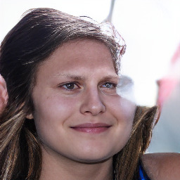
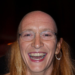
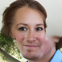
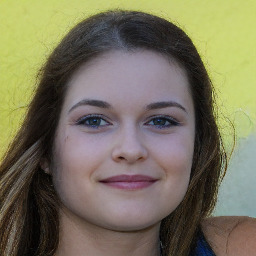
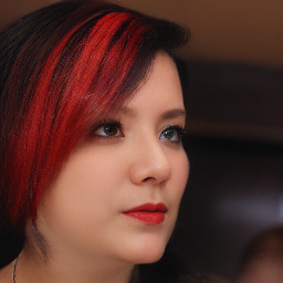
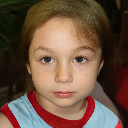
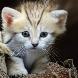
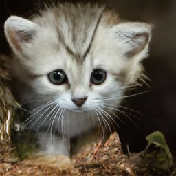
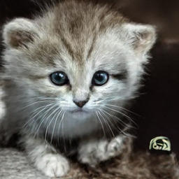
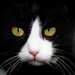
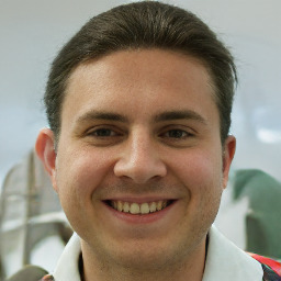
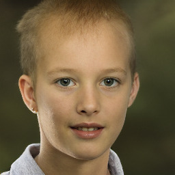
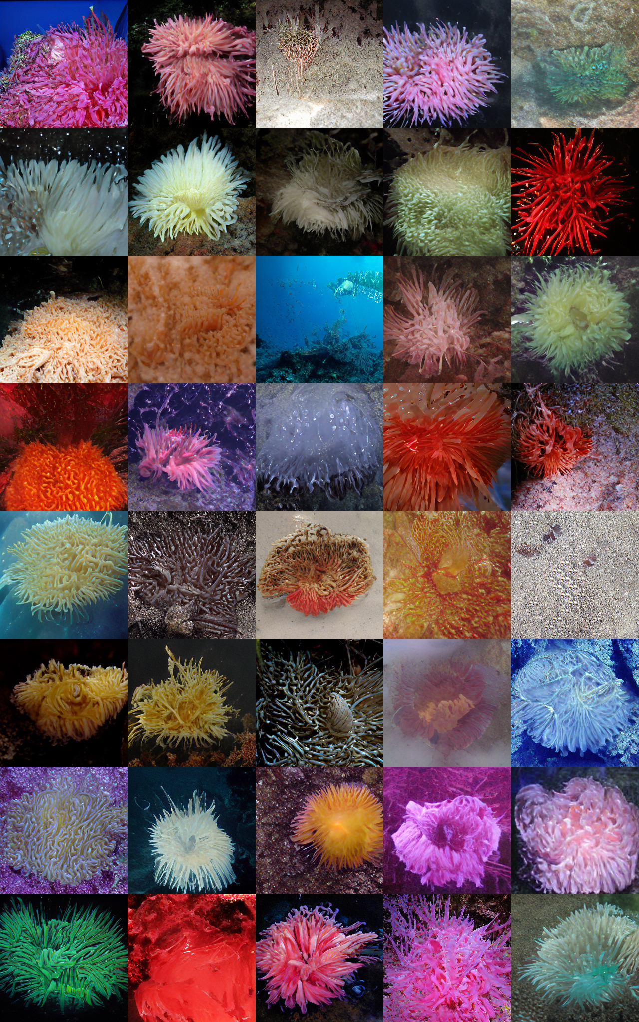
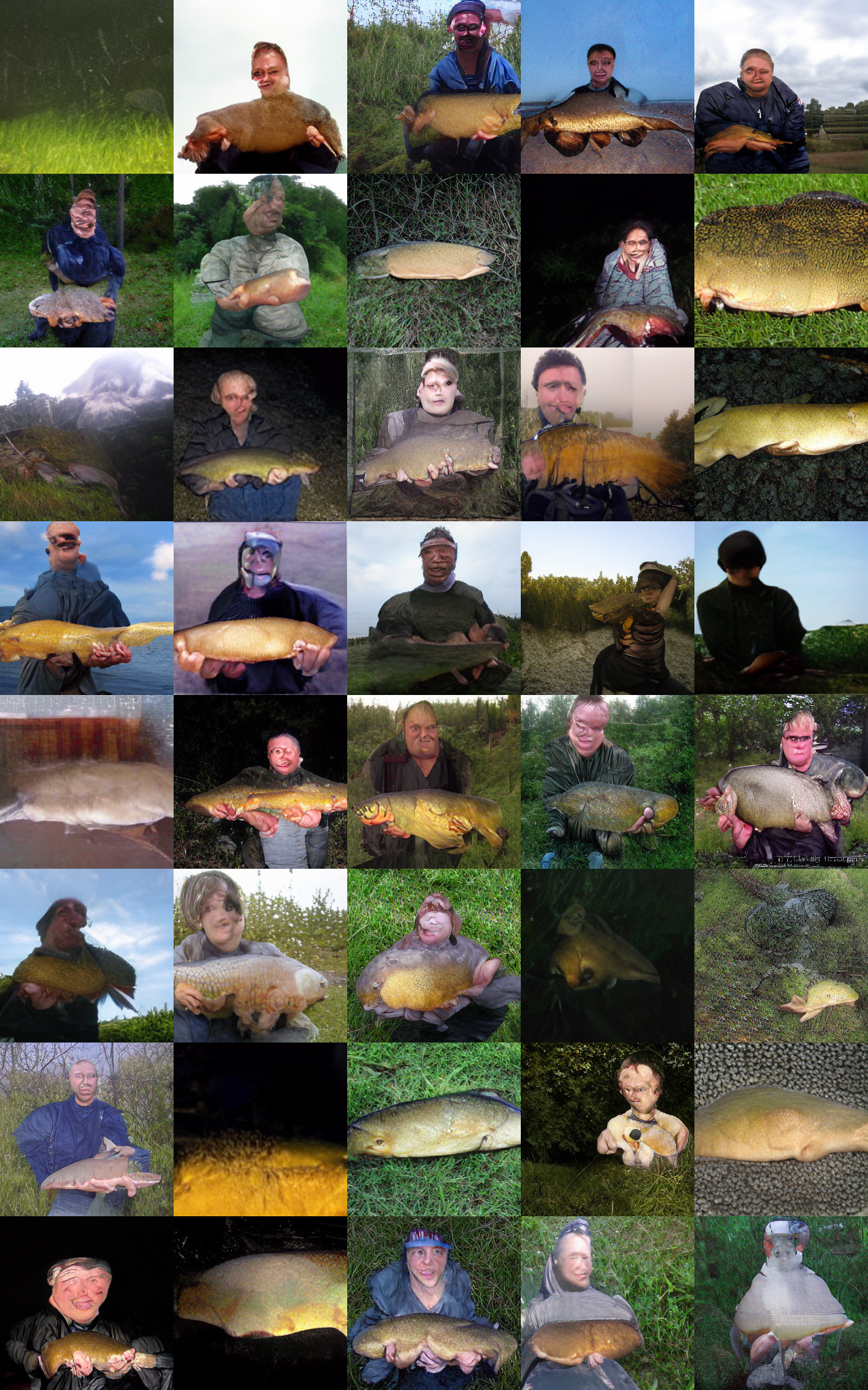
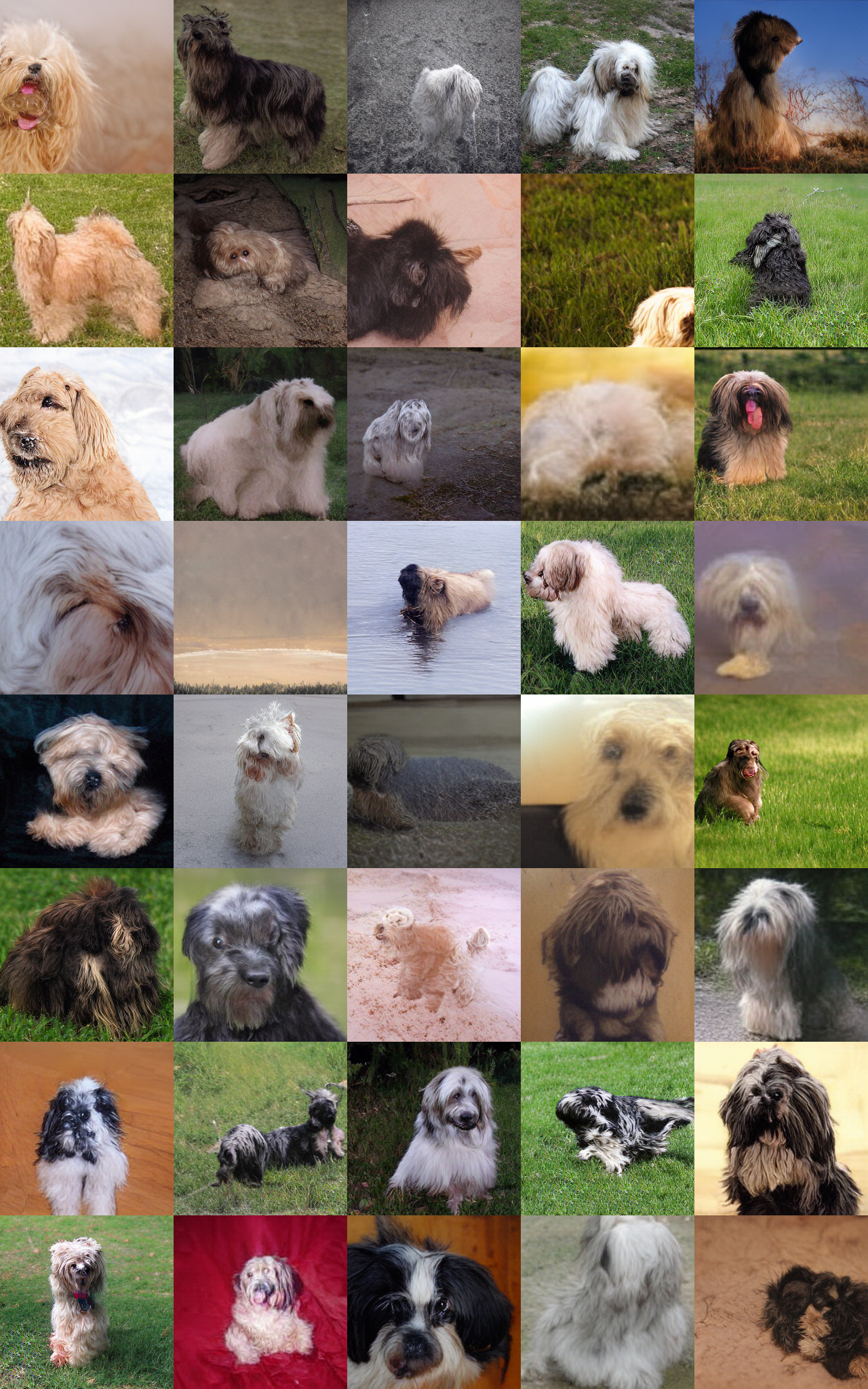
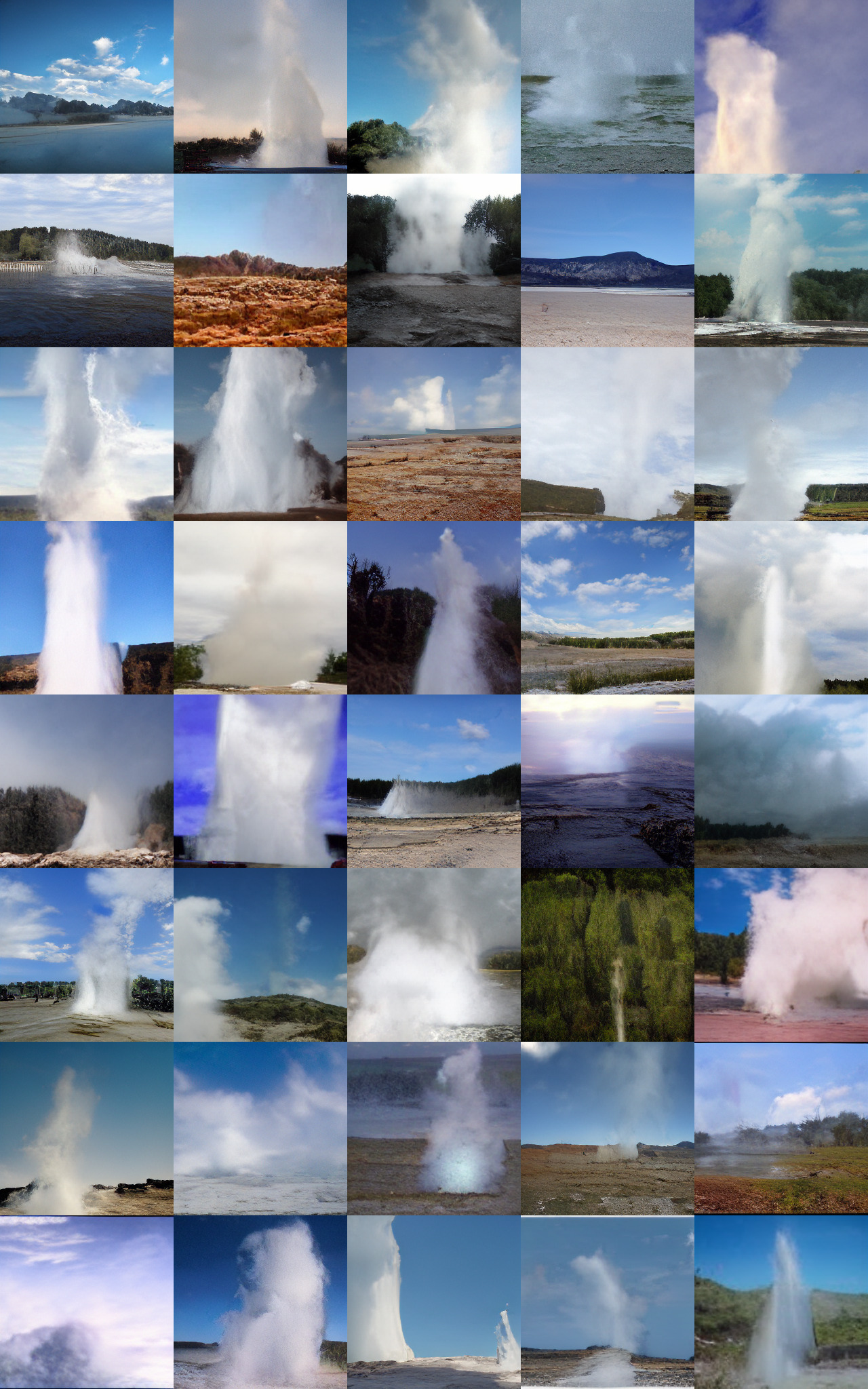
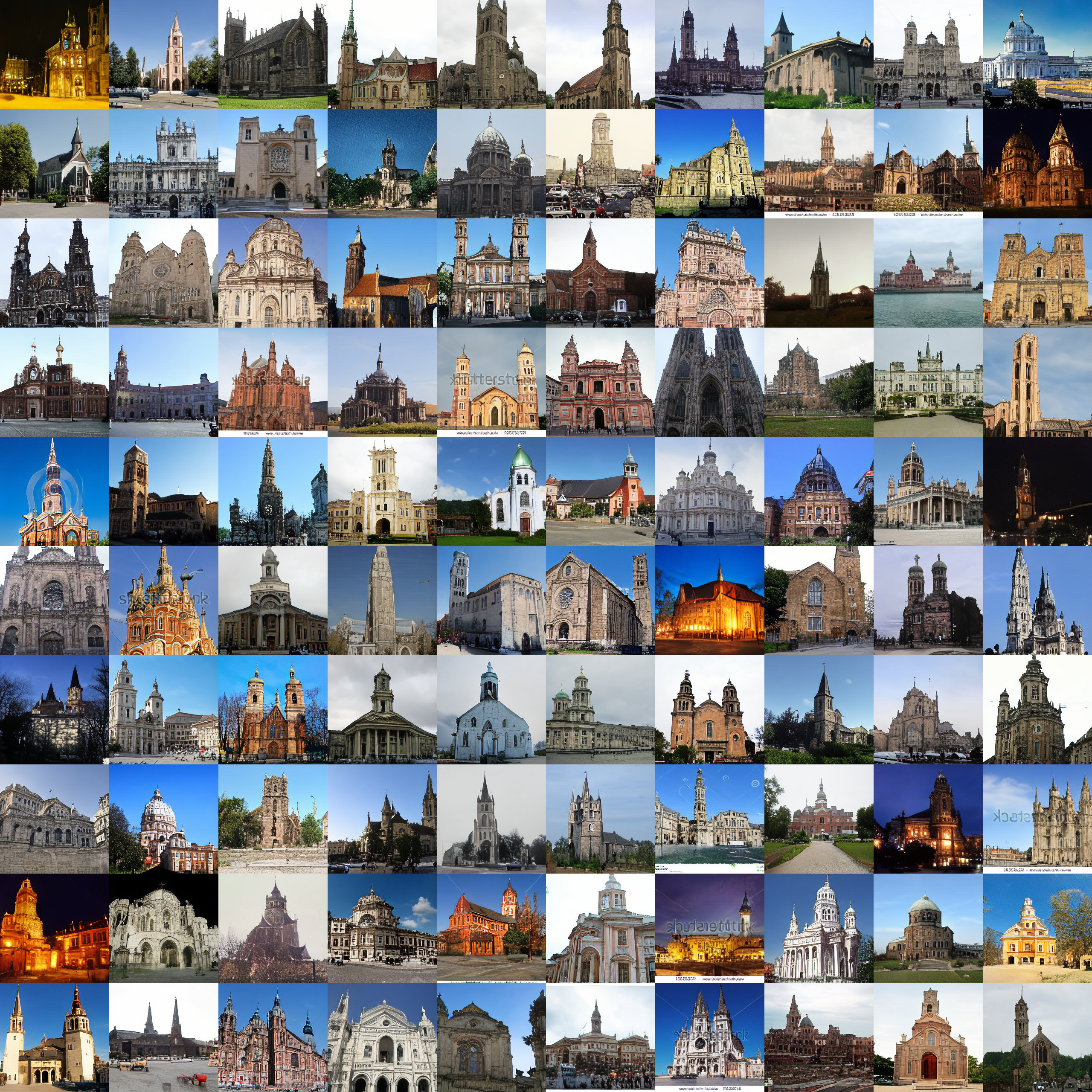
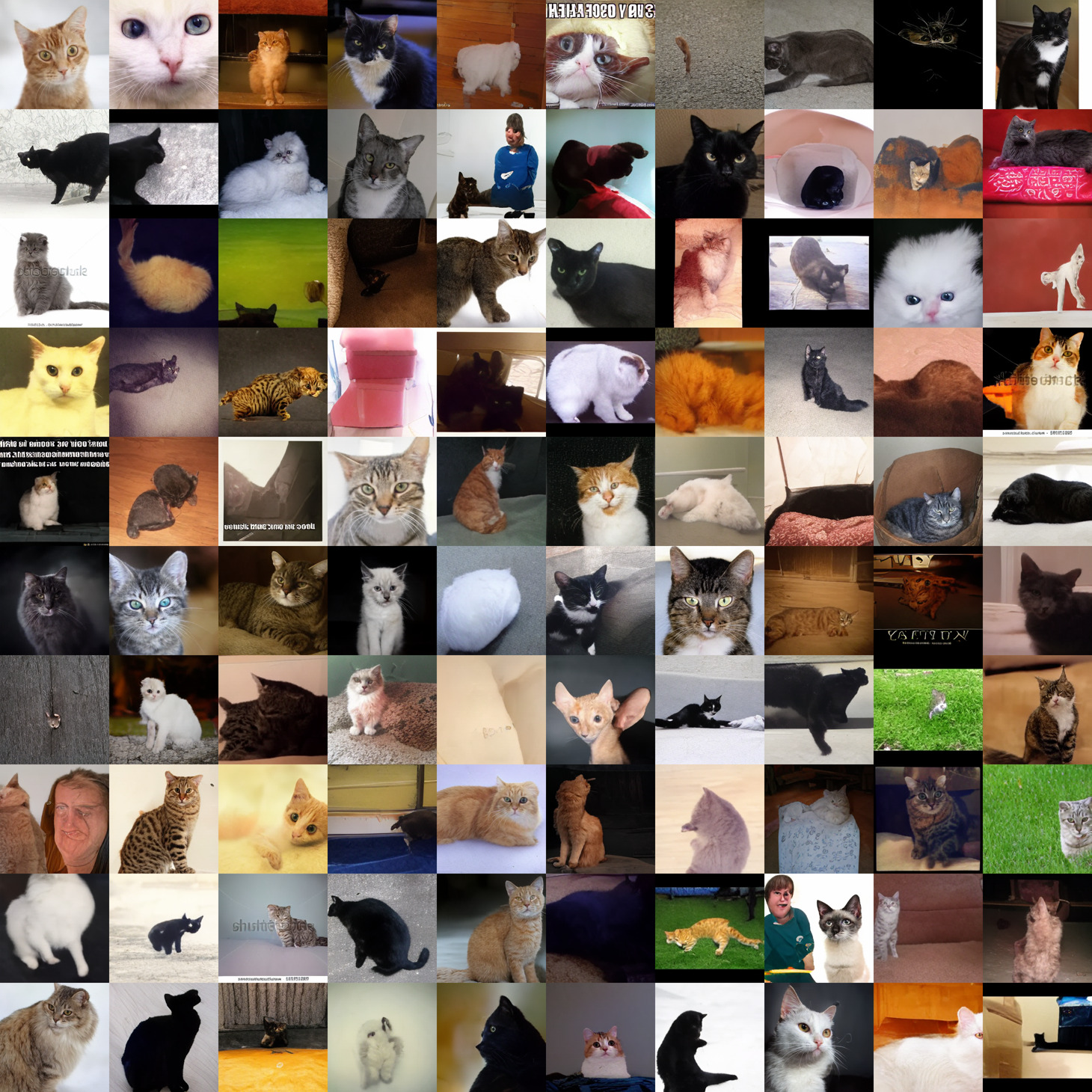
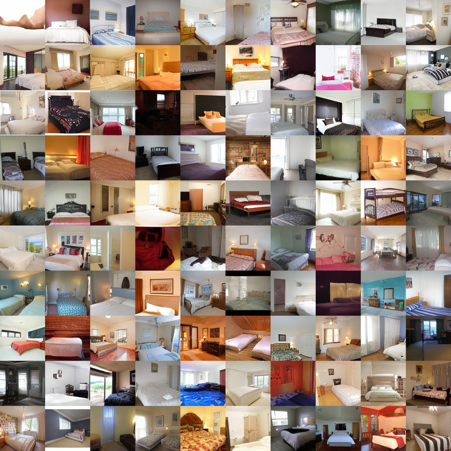
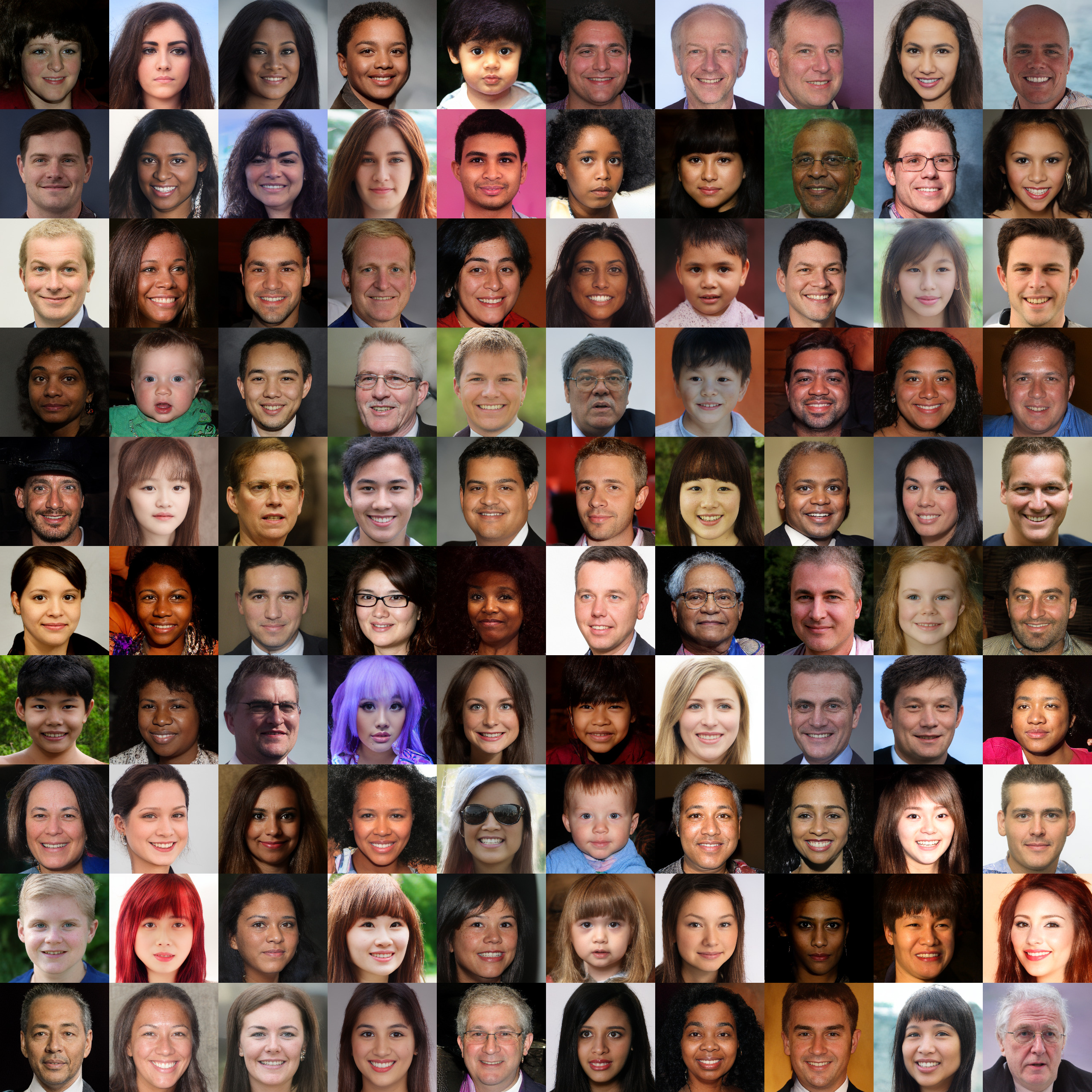
In this section we present qualitative and quantitative results on images synthesized by our approach. We train models at resolution for unconditional generation on FFHQ [30], LSUN -Cats, -Churches and -Bedrooms [76] and on class-conditional synthesis on ImageNet (cIN) [11].
| ImageBART | DDPM | SSDE | |||||||
| Churches | |||||||||
| Cats | |||||||||
| cIN (c14) | |||||||||
| cIN (c323) | |||||||||
| cIN (c963) | |||||||||
| rejection rate for cIN sampling | ||||
| 1.0 | 0.5 | 0.25 | 0.05 | |
| FID | 21.19 | 13.12 | 9.77 | 7.44 |
| IS | 61.6 | 109.5 | 146.2 | 273.5 |
Effective Discrete Representations Learning the full hierarchy as described in Eq. (2) and without unnecessary redundancies in the data requires to first learn a strong compression model via the objective in Eq. (4). [18] demonstrated how to effectively train such a model and we directly utilize the publicly available pretrained models. For training on LSUN, we finetune an ImageNet pretrained model for one epoch on each dataset. As the majority of codebook entries remains unused, we shrink the codebook to those entries which are actually used (evaluated on the validation split of ImageNet) and assign a random entry for eventual outliers. This procedure yields an effective, compact representation on which we subsequently train ImageBART.
Training Details As described in Sec. 3.3, we use an encoder-decoder structure to model the reverse Markov Chain , where the encoder is a bidirectional transformer model and decoder is implemented as an AR transformer. As the context for the last scale is pure noise, we employ a decoder-only variant to model . Furthermore, to account for the different complexities of the datasets, we adjust the number of multinomial diffusion steps for each dataset accordingly. For FFHQ we choose a chain of length , such that the total model consists of (i) the compression stage and (ii) transformer models trained in parallel via the objective described in Eq.(7). Similarly, we set for each of the LSUN models and for the ImageNet model.
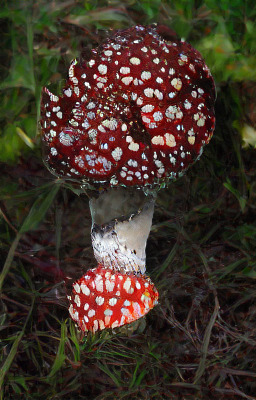
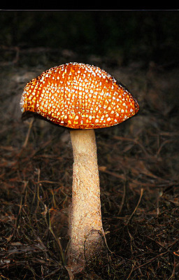
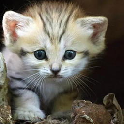
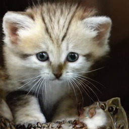
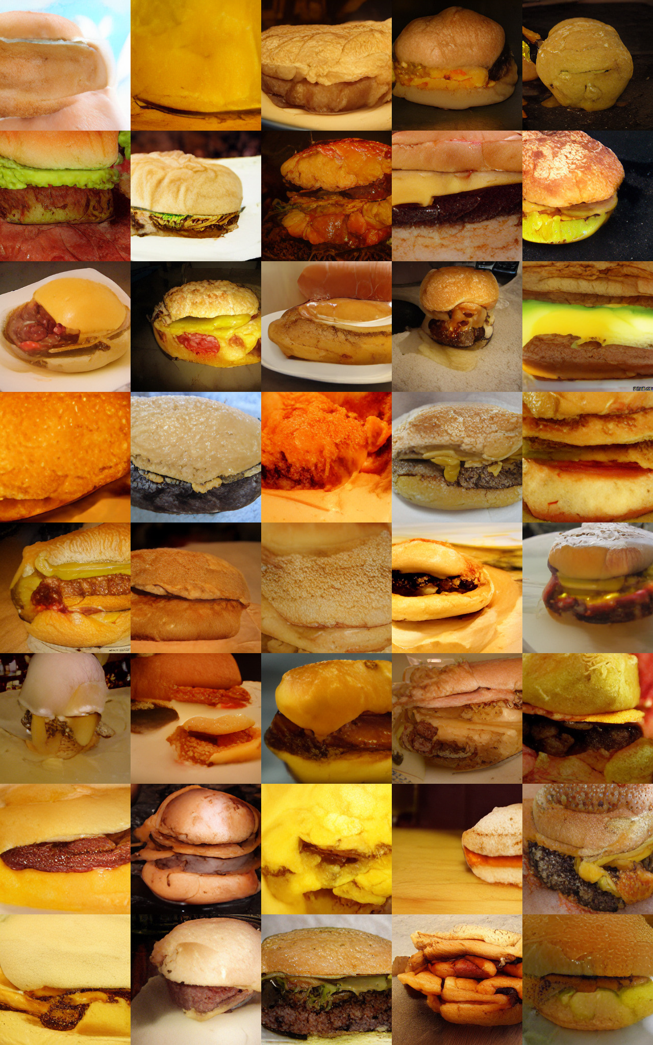
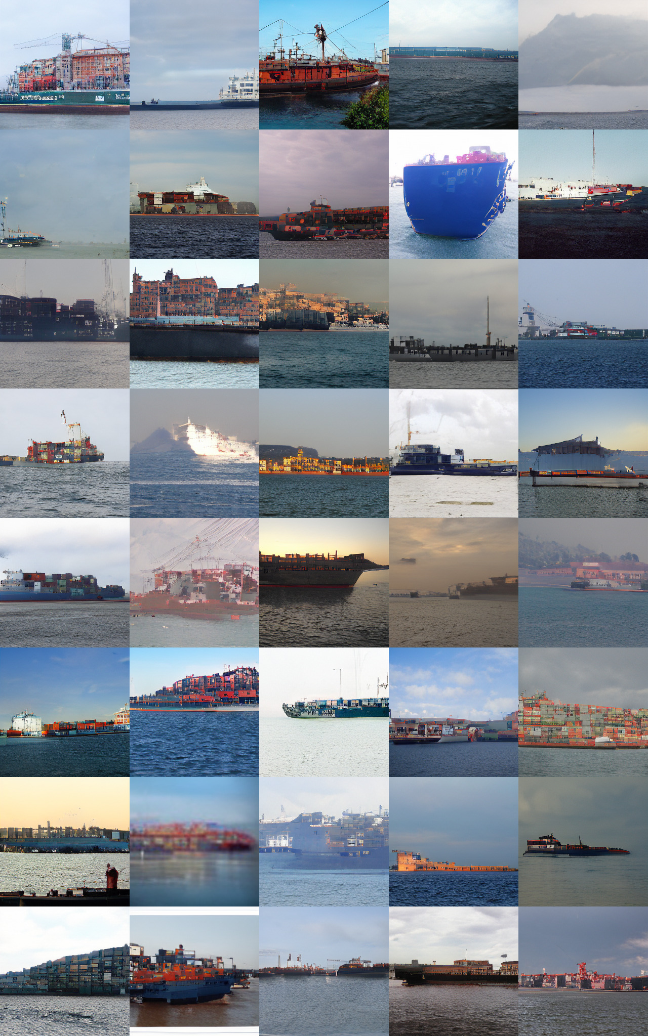
Results For each of these settings, Fig. 2 depicts samples of size generated with ImageBART and a single pass through the learned Markov Chain, demonstrating that our model is able to produce realistic and coherent samples. This is further confirmed by a quantitative analysis in Tab. 1, where we compare FID scores of competing likelihood-based and score-based methods such as TT [18] and DDPM [26]. Regarding other works on diffusion models such as [26] and [65] operating directly in pixel space, we observe that these approaches perform roughly equivalently well in terms of FID for datasets of low complexity (e.g. LSUN-Bedrooms and-Churches). For more complex datasets (LSUN-Cats, cIN), however, our method outperforms these pixel-based approaches, which can also be seen qualitatively on the right in Tab. 1. See Fig. 20 for a comparison on ImageNet.
4.2 Conditional Markov Chains for Controlled Image Synthesis
Being a sequence-to-sequence model, our approach allows for flexible and arbitrary conditioning by simply preprending tokens, similar to [18, 53]. More specifically, each learned transition of the Markov chain is then additionally conditioned on a representation , e.g. a single token in the case of the class-conditional model of Sec. 4.1. Note that the compression model remains unchanged.
Text-to-Image Synthesis
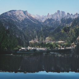
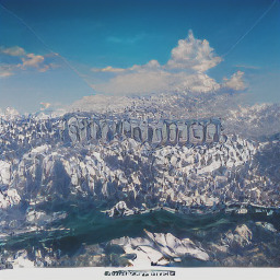
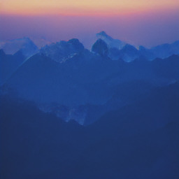
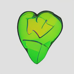
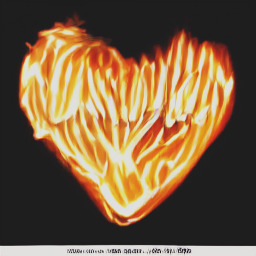
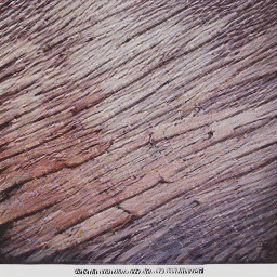
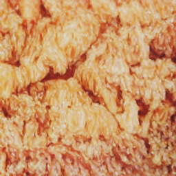
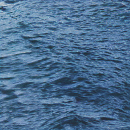
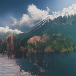
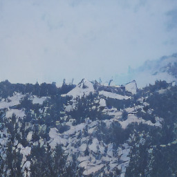
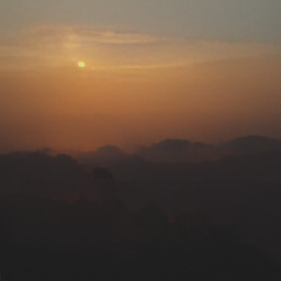
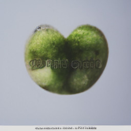
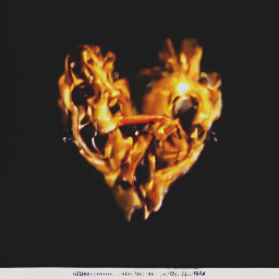
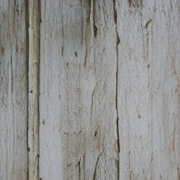
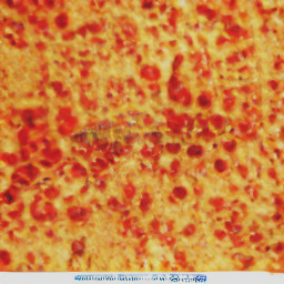
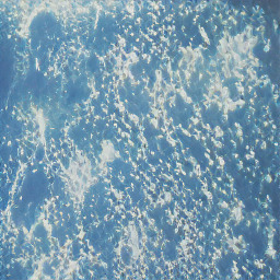
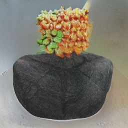
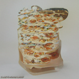
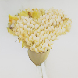
| Mountains and hills ___ | ___ in the shape of a heart. | The texture of ___ | ||||||
| reflecting on a surface./ | covered in snow./ | during sunrise. | An apple | An avocado | Flames | wood. | pizza. | water. |
 |
 |
 |
 |
 |
 |
 |
 |
 |
 |
 |
 |
 |
 |
 |
 |
 |
 |
Besides class-conditional modeling on ImageNet, we also learn a text-conditional model on Conceptual Captions (CC) [61, 48]. We obtain by using the publicly available tokenizer of the CLIP model [52], yielding a conditioning sequence of length 77. To model the dataset, we choose and thus train transformer models independently. For the , we directly transfer the compression model from Sec. 4.1, trained on the ImageNet dataset.
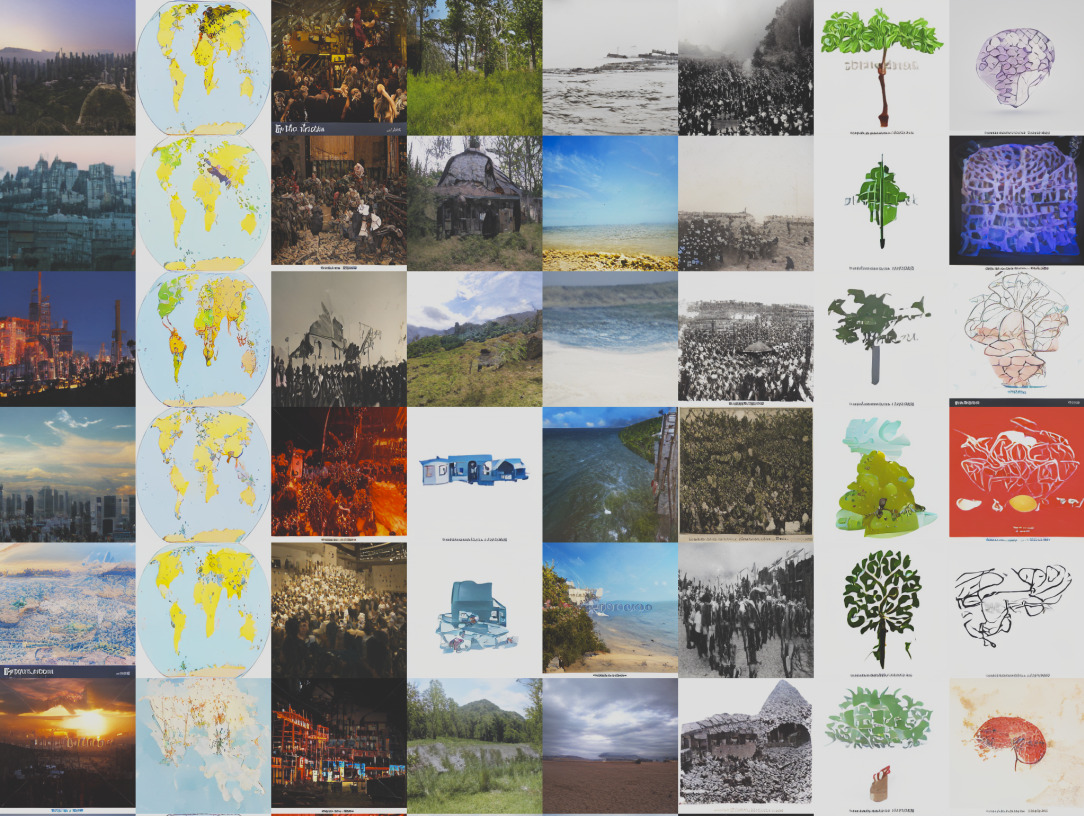
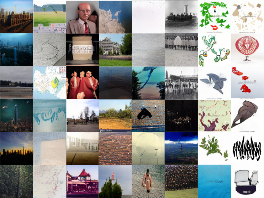
Fig. 3 visualizes synthetic samples obtained with this model for various “image-cloze” tasks. Our resulting model is able to attend to semantic variations in the conditioning sentence (e.g. a change of weather for imagery of mountains) and renders the corresponding images accordingly. In Tab. 2, we evaluate FID [25] and Inception Scores (IS) [58] to measure the quality of synthesized images, as well as cosine similarity between CLIP [52] embeddings of the text prompts and the synthesized images to measure how well the image reflects the text. ImageBART improves all metrics upon [18]. Fig. 21 in the supplement provides corresponding qualitative examples for user-defined text inputs.
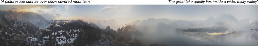
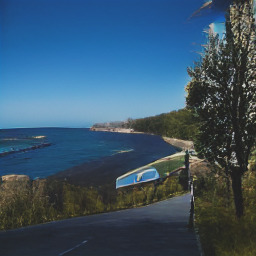
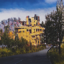
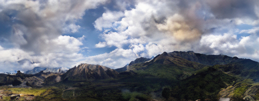
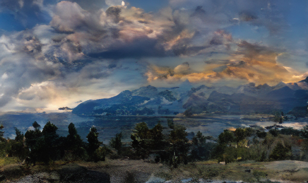
Resolutions Beyond Pixels. Our approach is not restricted to generating images of size pixels. Although trained on a fixed resolution, we can apply our models in a patch-wise manner, where we use the sliding attention window of [18] for each scale . As we now incorporate more and more global context while decoding with the Markov chain (which can be thought of as widening a noisy receptive field), ImageBART is able to render consistent images in the megapixel regime. See for example Fig. 4, where we use our text-conditional model to render an image of size pixel and interpolate between two different text prompts. More examples, especially also for semantically guided synthesis, can be found in Sec. A.2.
4.3 Beyond Conditional Models: Local Editing with Autoregressive Models
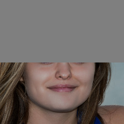
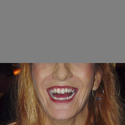
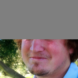
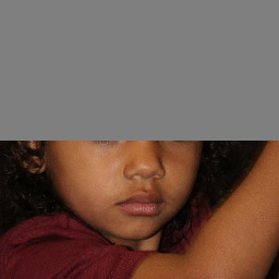
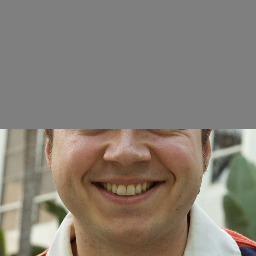
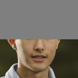
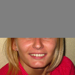
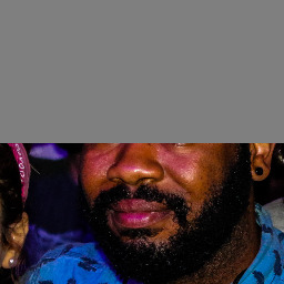
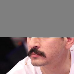
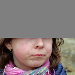
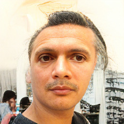
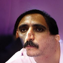
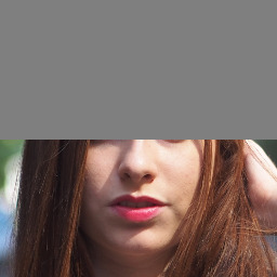
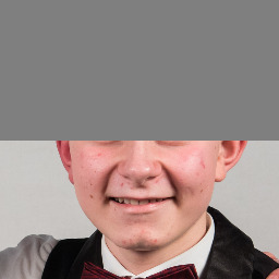
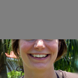
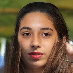
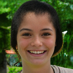
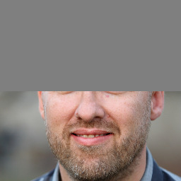
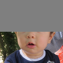
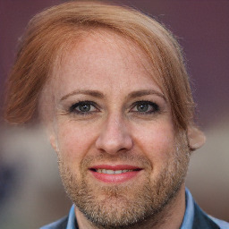
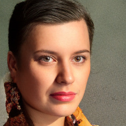
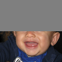
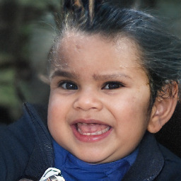
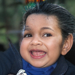
Recent autoregressive approaches, which use a CNN to learn a discrete representation [71], partially alleviate the issues of pixel-wise autoregressive models by working on larger image patches. However, as we show in Fig. 5, even approaches which use adversarial learning to maximize the amount of context encoded in the discrete representation [18] cannot produce completions of the upper half of an image which are consistent with a given lower half.
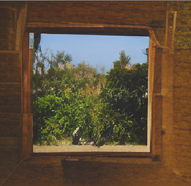
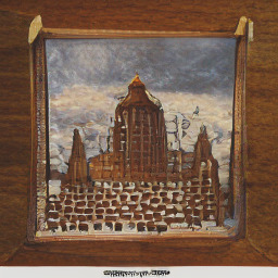
While our approach also models each transition autoregressively from the top-left to the bottom-right, the ability to attend to global context from the previous scale enables consistent completions of arbitrary order, e.g. right-to-left. To achieve this, we mask the diffusion process as described in Sec. A.3. For a user-specified mask (e.g. the upper half of an image as in Fig. 5), this results in a forward-backward process , which, by definition, leaves the unmasked context intact. The reverse process then denoises the unmasked entries to make them consistent with the given context.
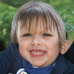
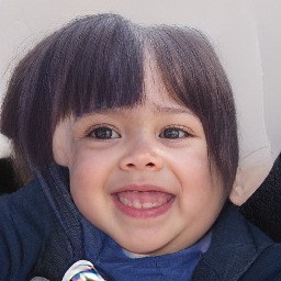
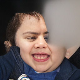
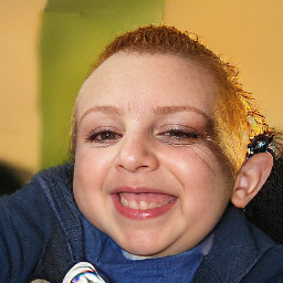
Fig. 5 (bottom) visualizes this mixing process, where we use a model with . The first column shows the masked input. To start the process we set all masked entries to random entries. The first two columns then show (decoded) samples from the masked reverse processes and , which still display inconsistencies. The remaining columns show the trajectory of the process , which demonstrates how the model iteratively adjusts its samples according to the given context until it converges to a globally consistent sample. For illustration, we show the analog trajectory obtained with [18], but because it can only attend to unidirectional context, this trajectory is equivalent to a sequence of independent samples and therefore fails to achieve global consistency.
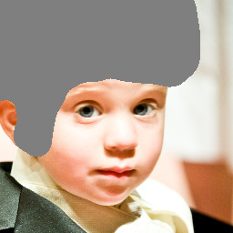
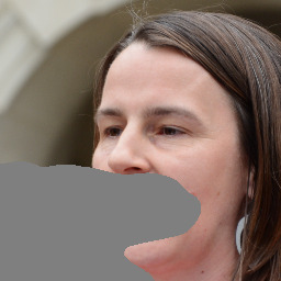
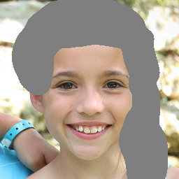
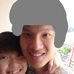
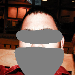
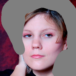
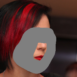
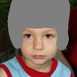
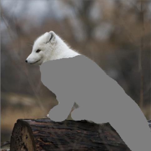
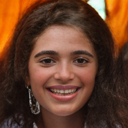
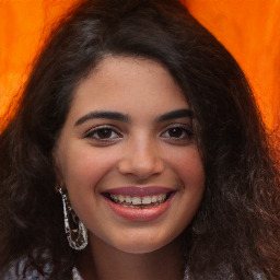
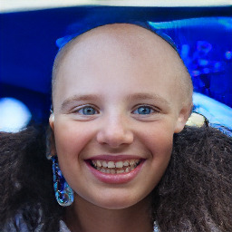
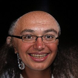
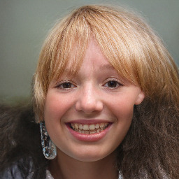
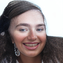
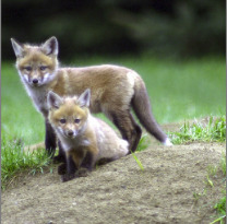
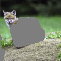
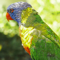
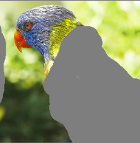
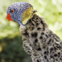
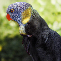
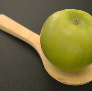
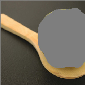
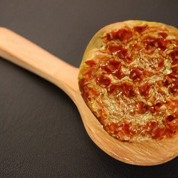
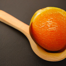
The masked process can be used with arbitrary masks, which enables localized image editing with free, hand-drawn masks as shown in Fig. 6. Note that our model does not need to be trained specifically for this task, which also avoids generalization problems associated with training on masks [78]. Combining this property with the conditional models from Sec. 4.2 allows for especially interesting novel applications, where local image regions are modified based on user specified class or text prompts, as shown in Fig. 7.
| Masked Input | TT [18] | ImageBART | ||||||
 |
 |
 |
 |
 |
 |
 |
 |
 |
| Input | Iterative Refinement According to Global Context | |||||||
ImageBART
TT [18] |
 |
 |
 |
 |
 |
 |
 |
 |
 |
 |
 |
 |
 |
 |
 |
 |
 |
 |
 |
 |
 |
 |
 |
 |
 |
 |
 |
 |
 |
 |
 |
 |
 |
 |
 |
 |
 |
 |
 |
 |
 |
 |
 |
 |
 |
 |
 |
 |
 |
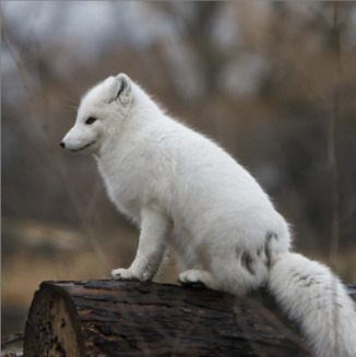
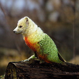
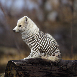
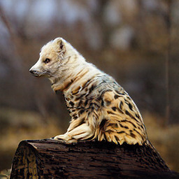
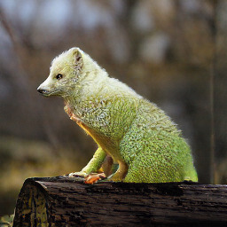
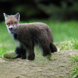
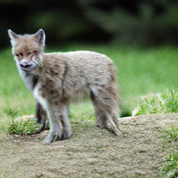
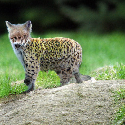
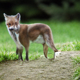
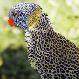
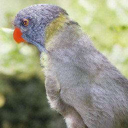
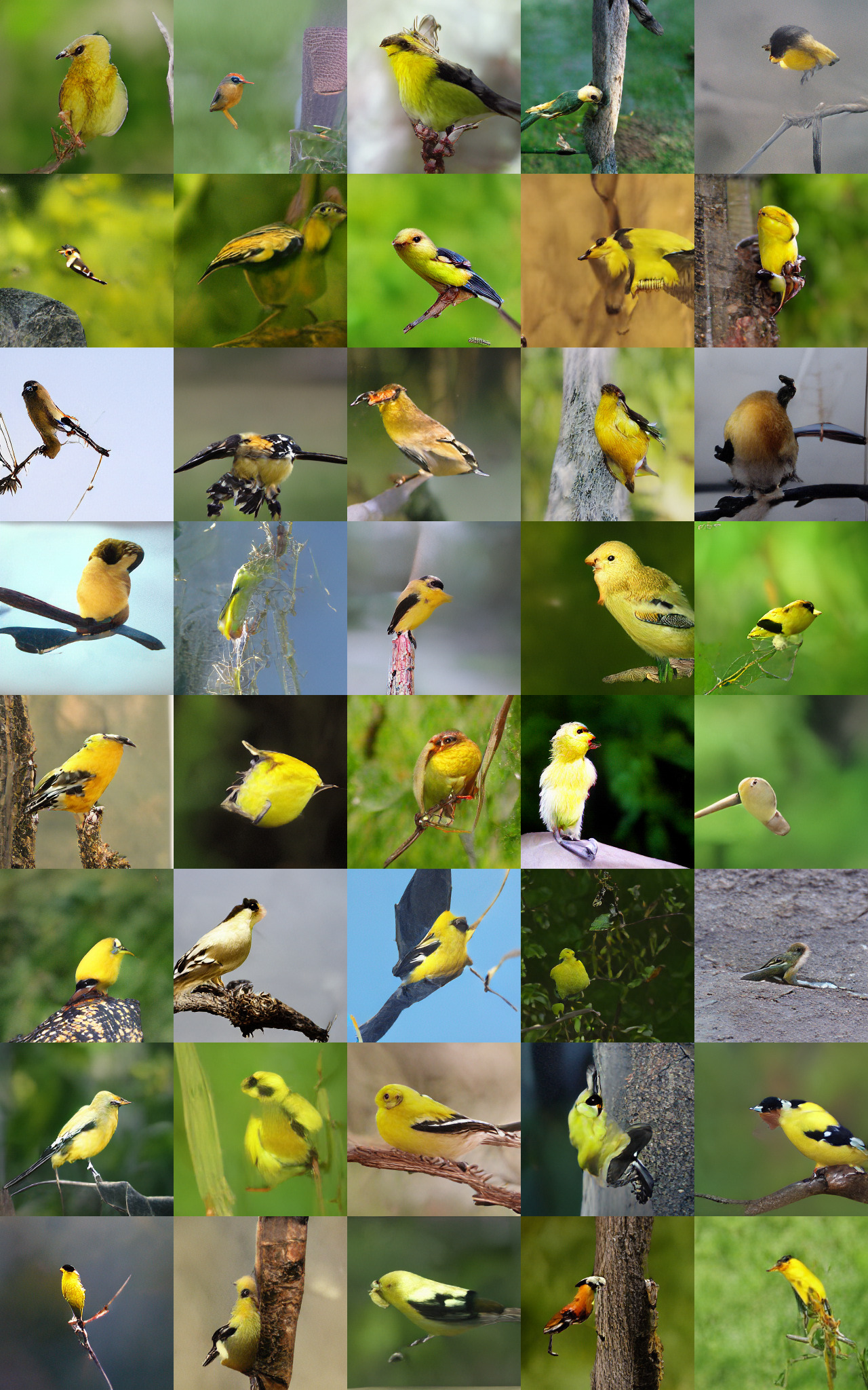
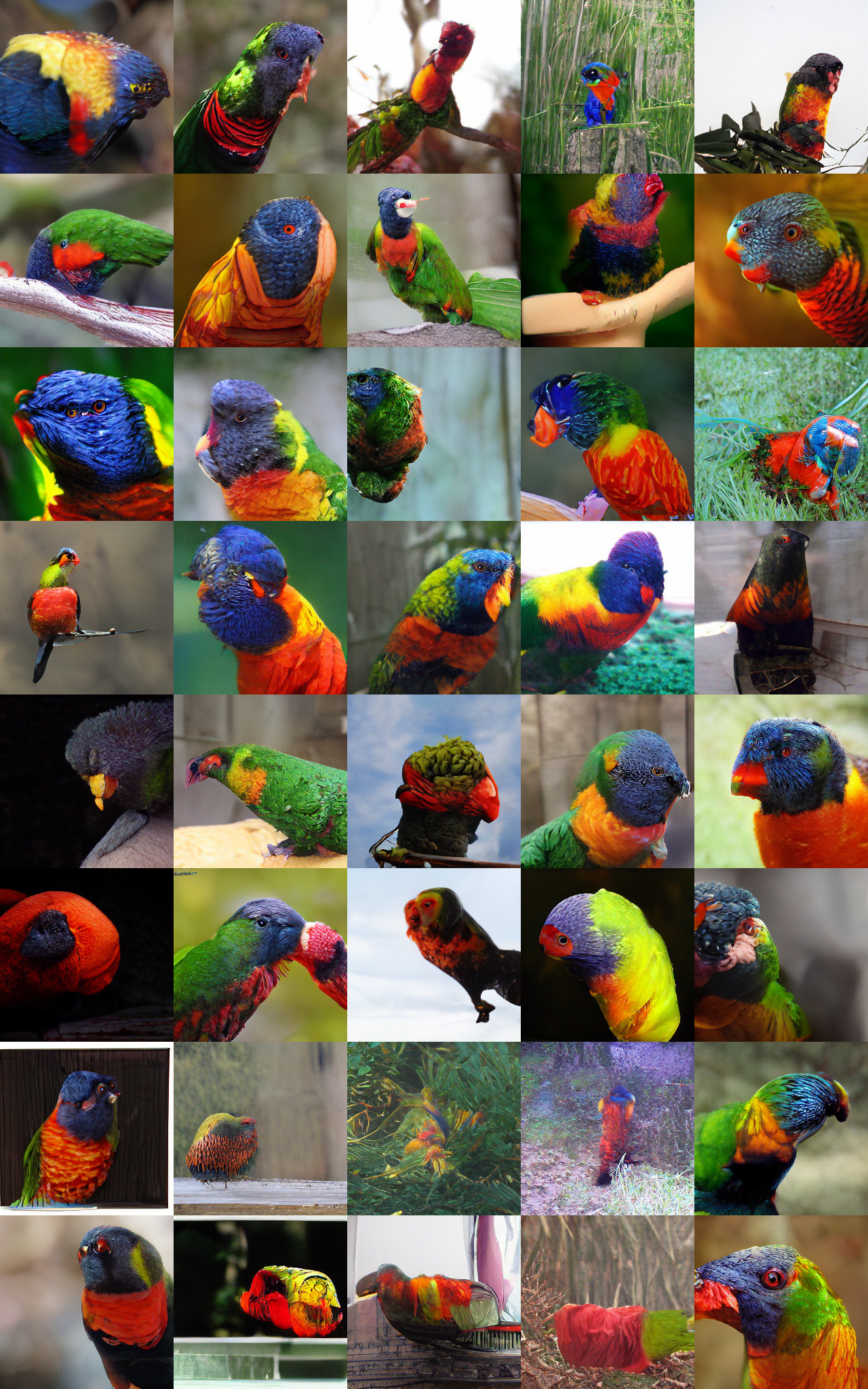
| Original | Masked | Guidance | |||
| Arctic fox (c279) | Lorikeet (c90) | Zebra (c340) | Tiger (c292) | Green lizzard (c46) | |
 |
 |
 |
 |
 |
 |
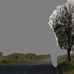
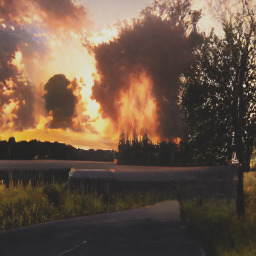
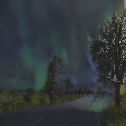
| ’Man standing on a road’ | ’A beautiful sunset.’ | ’Northern lights.’ | ’The road leads straight | ’A small city.’ | |
| ’in nature in summer.’ | to the coast.’ | ||||
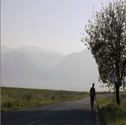 |
 |
 |
 |
 |
 |
4.4 Ablations
On the Number of Diffusion Steps In this section we analyze the effect of varying the number of diffusion steps (denoted by ). To do so, we perform an experiment for unconditional training on the FFHQ dataset, where we train a Taming Transformers (TT) baseline (corresponding to the case within our framework) with 800M parameters and three variants of ImageBART with (2x400M), (4x200M) and (8x100M), respectively. Note that for a fair comparison, all models use the same first level for compression, and we fix the number of remaining parameters to 800M and distribute them equally across all scales. All models were trained with the same computational budget and evaluated at the best validation checkpoint.
In Tab. 3, we assess both the pure synthesis and the modification ability of ImageBART by computing FID scores on samples and modified images (in the case of upper half completion as in Fig. 5). For both tasks, we use a single pass through the reverse Markov chain. We observe that the modification performance increases monotonically with the number of scales, which highlights the improved image manipulation abilities of our approach. For unconditional generation, we observe a similar trend, although FID seems to plateau beyond .
Unconditional Generation method FID IS TT () 12.44 ImageBART () 12.55 ImageBART () 10.69 ImageBART () 10.81 Upper Half Completion method FID IS TT () 11.80 ImageBART () 9.25 ImageBART () 6.87 ImageBART () 6.64
Joint vs. Independent Training While it is possible to optimize Eq. (2) jointly across all scales, we found that training is more robust when training all scales independently. Besides the usual separation of training the compression model and the generative model , training the latter in parallel over multiple scales avoids the tedious weighting of the loss contribution from different scales; an often encountered problem in other denoising diffusion probabilistic models [26].
Efficiency with Less Decoder Layers As we implement the conditional transition probabilities with an encoder-decoder transformer architecture, we are interested in the effect of altering the ratio of encoder and decoder layers in the model. Recent work has provided evidence that it is possible to significantly reduce the number of decoder layers and thus also decrease autoregressive decoding speed while maintaining high quality [32].
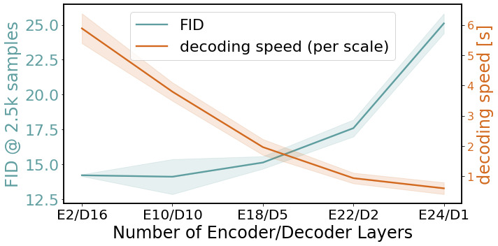
We perform an experiment on LSUN-Churches, where we analyze the effect of different layer-ratios on synthesis quality (measured by FID) and on decoding speed when fixing the total number of model parameters to 200M. The results in the left part of Fig. 8 confirms that it is indeed possible to reduce the number of decoder layers while maintaining satisfactory FID scores with higher decoding efficiency. We identity a favorable trade-off between four and six decoder layers and transfer this setting to our other experiments.
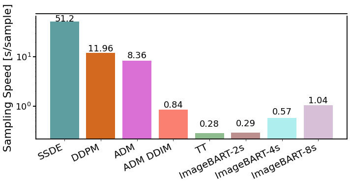
Finally, we compare our model in terms of sampling speed with the recent state-of-the-art generative diffusion [26, 65] and AR models [18]. The results are summarized in Fig. 8. While consistently being faster than all pixel-based models due to training in a compressed latent space, the increase in runtime w.r.t. [18] is moderate due to the use of encoder-decoder transformers, i.e., a a decrease in pure decoder layers. If a faster runtime is desired, the speed can be further increased by reducing the number of decoder layers even more, see also the discussion in Sec. A.5.
5 Conclusion
We have proposed ImageBART, a hierarchical approach to introduce bidirectional context into autoregressive transformer models for high-fidelity controllable image synthesis. We invert a multinomial diffusion process by training a Markov chain to gradually incorporate context in a coarse-to-fine manner. Our study shows that this approach (i) introduces a natural hierarchical representation of images, with consecutive levels carrying more information than previous ones. (see also Fig. 9). (ii) It alleviates the unnatural unidirectional ordering of pure autoregressive models for image representation through global context from previous levels of the hierarchy. (iii) It enables global and local manipulation of a given input, a feat previously out-of-reach for ARMs. (iv) We additionally show that our model can be efficiently conditioned on various representations, allowing for a large class of conditional image synthesis tasks such as semantically guided generation or text-to-image synthesis.
Appendix A Appendix
A.1 Hyperparameters & Implementation Details
A.1.1 Compression Models
| experiment | section | add. samples | effective size | fine-tuned from [18] | trained from scratch | compression rate |
| class-cond. ImageNet | 4.1 | Fig. 10,18,19 | 973 | ✗ | ✗ | |
| LSUN-Cats | 4.1 | Fig. 23 | 1014 | ✓ | ✗ | |
| LSUN-Churches | 4.1 | Fig. 22 | 1022 | ✓ | ✗ | |
| LSUN-Bedrooms | 4.1 | Fig. 24 | 1017 | ✓ | ✗ | |
| Conceptual Captions | 4.2 | Fig. 11 | 973 | ✗ | ✗ | |
| FFHQ | 4.1 | Fig. 25 | 548 | ✗ | ✓ | |
| Semantic FLICKR | A.2 | Fig. 12,13 | 973 | ✗ | ✗ |
We follow [18] and implement our image compression models as “VQGANs”. More specifically, we use the official implementation provided at https://github.com/CompVis/taming-transformers and fine-tune the publicly available model for experiments on LSUN. For FFHQ, we train such a compression model from scratch. See Tab. 4 for an overview. As some of the codebook entries remain unused after training, we shrink the codebook to its effective size when training a generative model on top of it. For eventual entries not detected during evaluation on the subset, we assign a random entry.
A.1.2 Hierarchical Representations via Multinomial Diffusion
| experiment | length of chain | schedule () | effect. seq. length (full , , w/o cond.) |
| class-cond. ImageNet | |||
| LSUN-Cats | |||
| LSUN-Churches | |||
| LSUN-Bedrooms | |||
| Conceptual Captions | |||
| FFHQ | |||
| Semantic FLICKR |
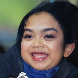
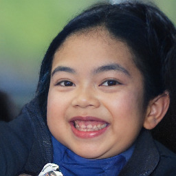
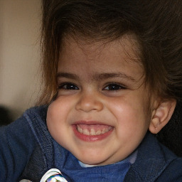
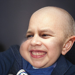
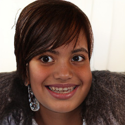
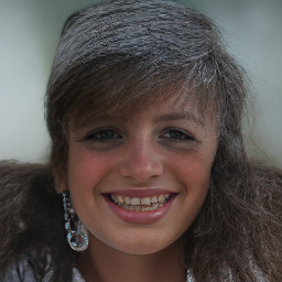
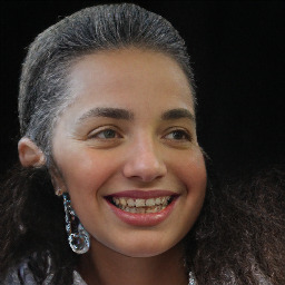
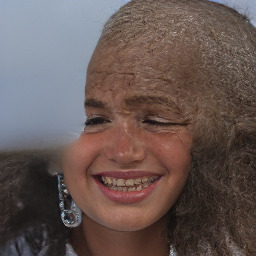
Tab. 5 lists the configurations of the multinomial diffusion processes for each experiment described in this work (see also Tab. 4). Note that all representations for have the same spatial resolution, but since each forward diffusion process gradually removes information, we obtain a coarse-to-fine hierarchy. On average, level will contain valid entries, which we denote as the effective sequence length in Tab. 5. Thus, ImageBART can also be interpreted as a generative compression model as illustrated in Fig. 9: By trading perfect reconstruction quality for compression, one can obtain a significantly shorter sequence, still representing a visually plausible image. This provides the basis for learning a generative model that does not waste capacity on redundancies in the data [15] and the compressed space significantly lowers the computational demands for training and decoding.


A.1.3 Reverse Diffusion with Transformer Models
| experiment | num. parameters [M] | num. layers (encoder/decoder) | embed. dim. (encoder & decoder) |
| class-cond. ImageNet | |||
| LSUN-Cats | |||
| LSUN-Churches | |||
| LSUN-Bedrooms | |||
| Conceptual Captions | |||
| FFHQ | |||
| Semantic FLICKR |
ImageBART is a learned Markov chain, trained to reverse the multinomial diffusion process described in Eq. (5). We can efficiently model the conditionals with a sequence-to-sequence model and follow [72, 42] to implement with an encoder-decoder architecture. Tab. 6 summarizes the hyperparameters used to implement the conditionals for each experiment. For comparison, the models in Tab. 1 contain 115M (VDVAE), 255M (DDPM), 30M (StyleGAN2), 158M (BigGAN), 448M (DCT) and 600M (TT) parameters.
A.1.4 Hardware
A.2 Details on Conditional Experiments
|
 |
 |
 |
 |
 |
 |
 |
|
 |
 |
 |
 |
 |
 |
 |
 |
 |
 |
 |
|
|
 |
 |
 |
 |
 |
 |
 |
 |
 |
 |
|
 |
 |
 |
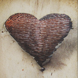
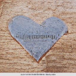
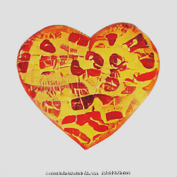
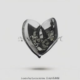
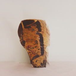
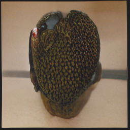
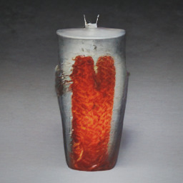
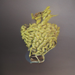
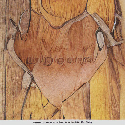
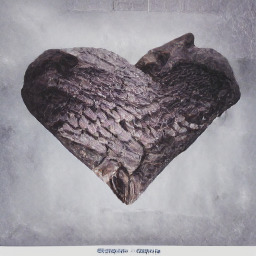
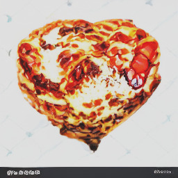
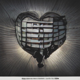
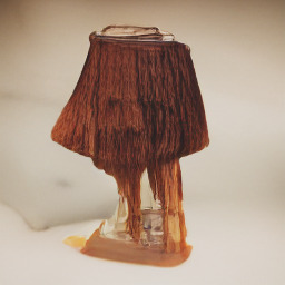
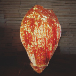
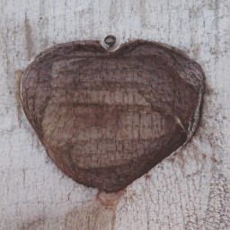
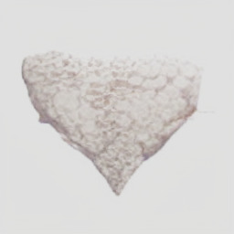
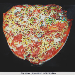
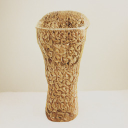
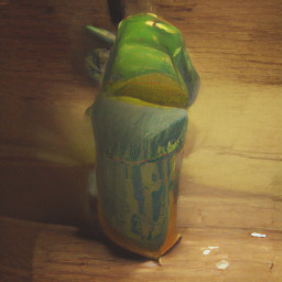
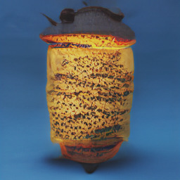
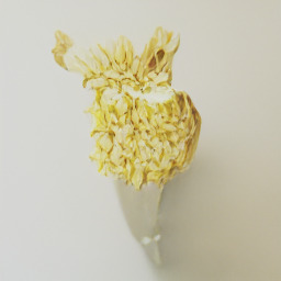
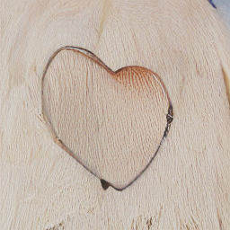
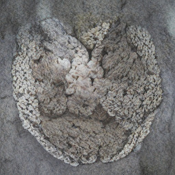
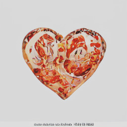
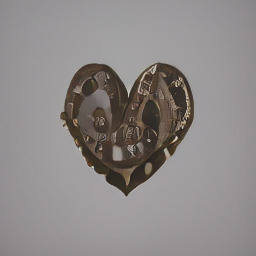
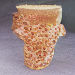
| A heart made of ___. | A vase made of ___. | ||||||
| wood | stone | pizza | metal | wood | avocado | pizza | pasta |
 |
 |
 |
 |
 |
 |
 |
 |
 |
 |
 |
 |
 |
 |
 |
 |
 |
 |
 |
 |
 |
 |
 |
 |
 |
 |
 |
 |
 |
 |
 |
 |
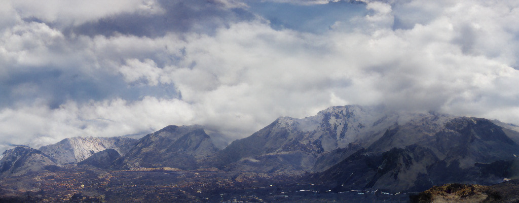
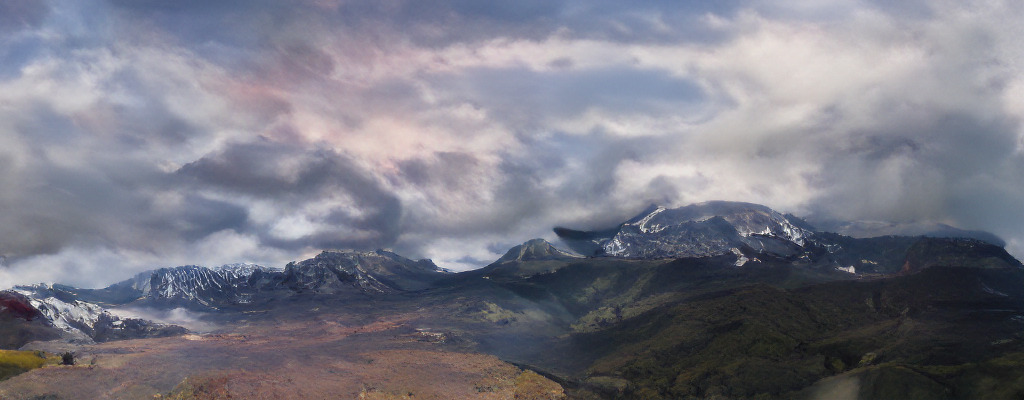
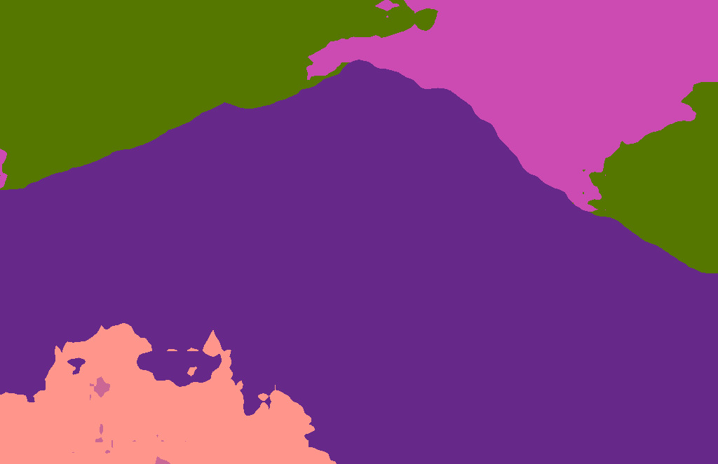
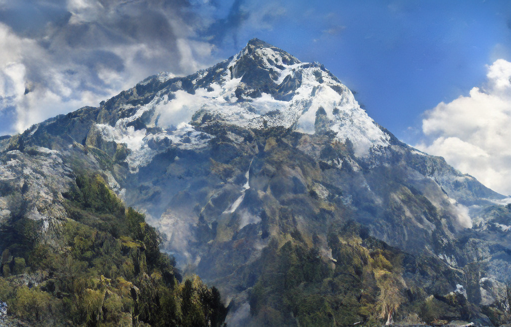
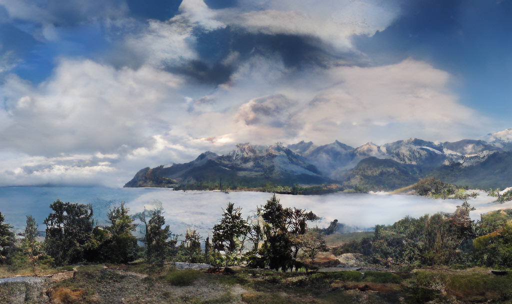
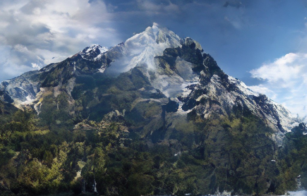
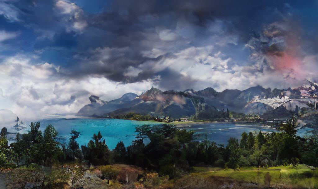
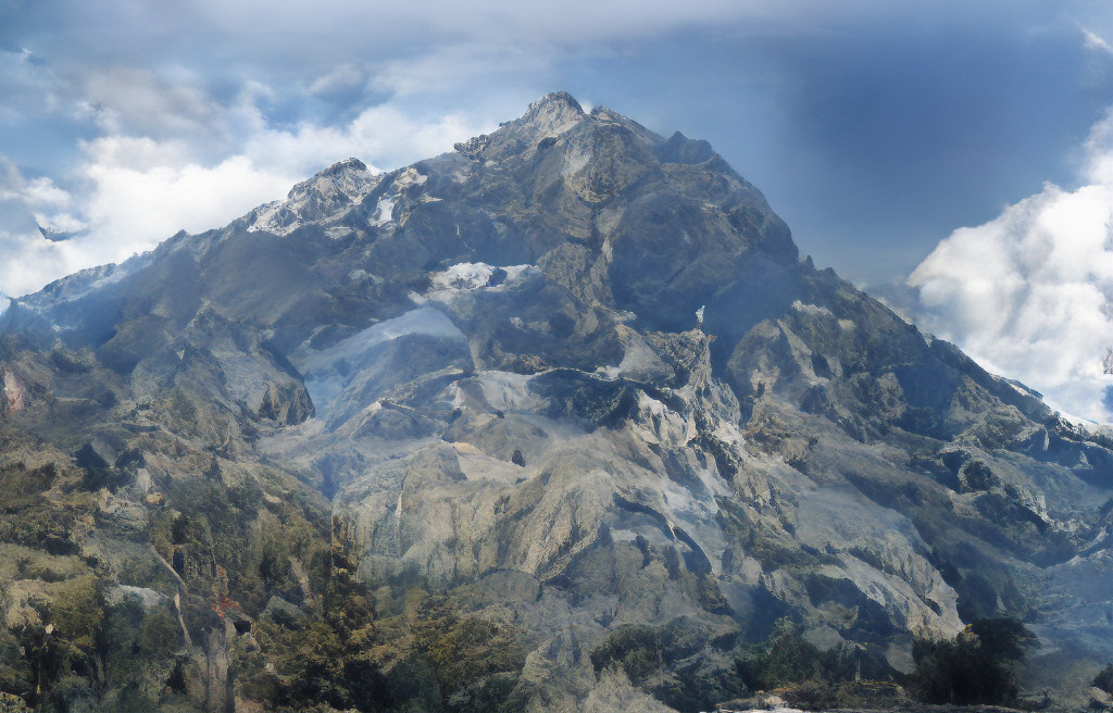
Semantically Guided Synthesis In addition to class- and text-conditional generative modeling, we apply our model to semantically guided synthesis of landscape images [50]. To achieve this we follow [18] and use the discrete representation of an autoencoder model trained on segmentation masks as conditioning for our models . However, since simply prepending here doubles the total length, which means a fourfold increase in complexity in the attention mechanism, we exploit the fact that the segmentation masks and the images (or their representations) are aligned. More specifically, within the encoder-decoder architecture, we first produce two embeddings and for and , respectively, which are subsequently concatenated channel-wise, thereby keeping the sequence length of . With this modifications, we train a model with and individually optimize each scale similar to the unconditional training setting. Here again, we use the compression model pre-trained on ImageNet. For training, we randomly crop the images and semantic maps to size . For testing, however, we again use the sliding window approach of [18] (cf. Sec. 4.2), which enables us to generate high-resolution images of landscapes, as visualized in Fig. 12 and Fig. 13.

 |
 |
 |
 |
 |
 |
 |
 |
A.3 Masked Diffusion Processes for Local Editing


| Original | Masked | Guidance | |||
| Red fox (c277) | Brown Bear (c294) | White Wolf (c270) | Leopard (c289) | Gazelle (c353) | |
 |
 |
 |
 |
 |
 |
| Lorikeet(c90) | Snow Leopard (c288) | Doberman (c236) | Leopard (c289) | Arctic Fox (c279) | |
 |
 |
 |
 |
 |
 |
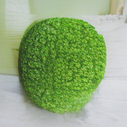
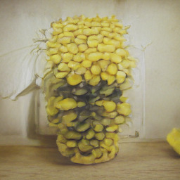
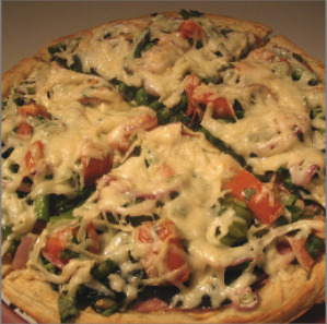
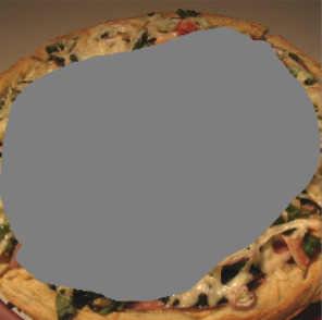
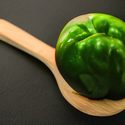
| Pizza (c963) | Carbonara (c959) | Meat loaf (c962) | Broccoli (c937) | Bell pepper (c945) | |
 |
 |
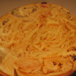 |
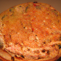 |
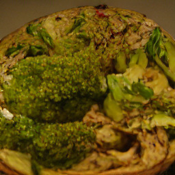 |
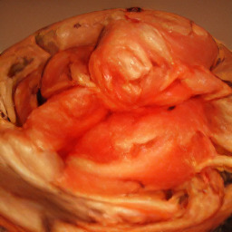 |
| Granny Smith (c948) | Pizza (c963) | Orange (c950) | Volleyball(c890) | Bell pepper (c945) | |
 |
 |
 |
 |
 |
 |
| Original | Masked | Guidance | ||
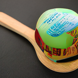
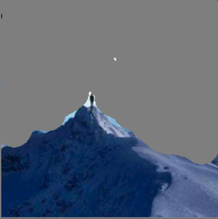
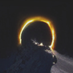
| ’Man standing on a mountain.’ | ’Solar Eclipse.’ | ’Sunrise.’ | ’Moonlight’ | |
 |
 |
 |
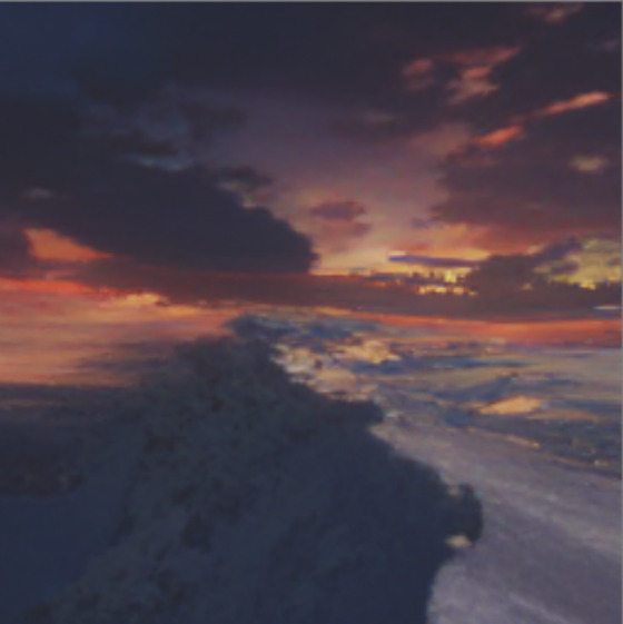 |
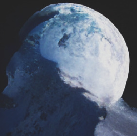 |
| ’The piece of paper.’ | ’A pencil sketch.’ | ’A forest behind the window.’ | ’Oil painting of a cathedral.’ | |
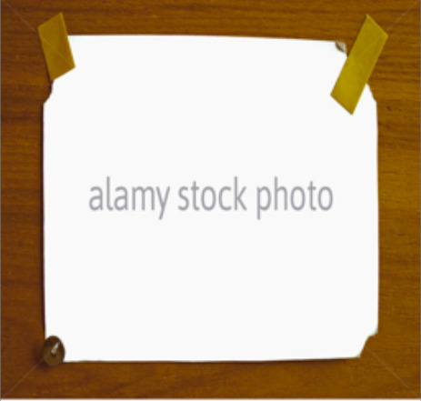 |
 |
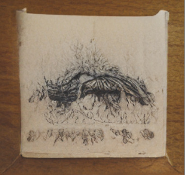 |
 |
 |

Previous autoregressive approaches [69] model images directly as a sequence of pixels from the top-left to the bottom-right. Thus, when generating a pixel, only context from neighbors to the left and above can be taken into account. While more recent approaches, which use a CNN to learn a discrete representation that is subsequently modeled autoregressively [71, 18], improve this situation because elements of the representation now correspond to image patches, Fig. 5 showed that these models still fail to generate completions of the upper half of an image which are consistent with a given lower half.
While our approach also models each transition autoregressively from the top-left to the bottom-right, each transition additionally has access to global context from the previous step. We aim to exploit this fact to obtain novel applications such as consistent completions of upper halfs and, more generally, completions with respect to an arbitrary mask. For any such mask, let denote the result of downsampling it to the size of using nearest-neighbor-interpolation, such that gives the positions where context should be used, and gives the positions where new content should be generated. We then define the masked forward process,
| (10) |
which only diffuses masked entries, and the masked reverse process,
| (11) |
which only denoises masked entries. By definition, running this process forward and then backward again represents the identity on umasked entries such that the given context remains constant. We denote this forward-backward process that starts from a given and produces a sample ,
| (12) |
by and use it to sample with spatial conditioning information. Since it always leaves the unmasked context intact, the reverse process denoises the unmasked entries to make them consistent with the given context.
Besides Fig. 5, 6 additional visualizations of this process can be found in Fig. 14. The top shows masked inputs (left), final results of upper completions obtained by [18] (middle) and by (right). The bottom visualizes the trajectory of the masked process, showing the masked input (leftmost column), denoised samples from (first column) and (second column), and every other sample from the forward-backward model . It demonstrates how the model iteratively incorporates global context from the previous scale to converge to a globally consistent sample at the very right. A visualization of the process on the class conditional ImageNet model is shown in Fig. 17. Additional examples for conditional samples from this process, as in Fig. 7, can be found in Fig. 15 and Fig. 16.
A.4 Limitations and Societal Impacts
Training deep generative models consumes a significant amount of energy (see also Sec. A.1 regarding the used hardware; the ImageNet model for example was trained for 19 days). With regard to the environment, it is important that we reduce the energy consumption as much as possible. To take a step in this direction, we followed previous works and relied on a strongly compressed, learned representation of images. Because we can fine-tune the corresponding encoder and decoder models from pre-trained ones, the costs for this step are largely amortized and subsequent levels of our hierarchy benefit from a drastically reduced sequence length. Nonetheless, it should be noted that such a strong compression scheme for images does not result in perfect reconstructions. For applications which require very high fidelity, such a level of compression might be unsuitable due to artifacts in the reconstructed images. Additionally, the use of adversarial learning in this stage can potentiate biases of datasets by its mode-seeking behavior. Both of these issues can be lessened with larger sequence lengths at the cost of higher energy requirements.
The transformer architecture which is used to model the transitions in our hierarchy is generally considered to be less biased compared to convolutional architectures. However, it also cannot benefit from useful inductive biases and therefore requires a large amount of data and resources to learn all required relationships. In early experiments, we noticed that on small datasets, such as CIFAR-10 [39], the transformer models overfit before they reach good performance. Thus, in its current implementation our approach requires datasets of sufficient size. Future works should evaluate different architectures, regularizations or augmentations to enable its use on small datasets. On the other extreme, we find that with large datasets, the main bottleneck is the computational resources that can be spent on the training of the transformer models. On the largest datasets, Conceptual Captions and ImageNet, we find that performance still improves after two weeks of training. Thus, consistent with other works on scaling up generative models, we expect that performance of our model will keep increasing with the available resources.
To ensure comparability with other approaches, we use standard benchmark datasets for deep generative models, even if some of them are known to contain offensive content [9].
A.5 Sampling Speed
Here, we discuss the effects of varying the number of encoder vs. decoder layers in ImageBART on sampling speed as presented in Sec. 4.4. On each diffusion scale, the encoder layers only have to run once whereas the decoder layers have to run times. This results in an approximate complexity of order , where is the complexity of a single transformer layer. The speedup from such an encoder-decoder transformer over a decoder only transformer with layers is therefore
| (13) |
A.6 Additional Samples & Nearest Neighbors
We provide additional samples from our models in Fig. 18-25. Additionally, we also provide nearest neighbors (measured in VGG feature space) for our FFHQ and LSUN-Churches models in Fig. 26 and Fig. 27, respectively.
 |
 |
 |
 |
 |
 |
 |
 |
| rate | ImageBART | TT [18] | ||||||||||
| 0.5 | ||||||||||||
| FID: 13.12 | FID: 10.26 | |||||||||||
| 0.25 | ||||||||||||
| FID: 9.77 | FID: 7.35 | |||||||||||
| 0.05 | ||||||||||||
| FID: 7.44 | FID: 5.88 | |||||||||||
| Sunset over the | Map of the world | Crowded scene | A small house | A photograph of a | A vector illustration of | ||
| skyline of a city. | in the year 2077. | in front of a pub. | in the wilderness. | beach. | crowd of people. | a tree. | the brain. |
| ImageBart | |||||||
 |
|||||||
| TT [18] |
 |
 |
 |


References
- Abdal et al. [2021] R. Abdal, P. Zhu, N. J. Mitra, and P. Wonka. Styleflow: Attribute-conditioned exploration of stylegan-generated images using conditional continuous normalizing flows. ACM Trans. Graph., 40(3), May 2021. ISSN 0730-0301. doi: 10.1145/3447648. URL https://doi.org/10.1145/3447648.
- Austin et al. [2021] J. Austin, D. Johnson, J. Ho, D. Tarlow, and R. v. d. Berg. Structured denoising diffusion models in discrete state-spaces. arXiv preprint arXiv:2107.03006, 2021.
- Bengio et al. [2015] S. Bengio, O. Vinyals, N. Jaitly, and N. Shazeer. Scheduled sampling for sequence prediction with recurrent neural networks. CoRR, abs/1506.03099, 2015.
- Brock et al. [2019] A. Brock, J. Donahue, and K. Simonyan. Large scale GAN training for high fidelity natural image synthesis. In Int. Conf. Learn. Represent., 2019.
- Brown et al. [2020] T. B. Brown, B. Mann, N. Ryder, M. Subbiah, J. Kaplan, P. Dhariwal, A. Neelakantan, P. Shyam, G. Sastry, A. Askell, S. Agarwal, A. Herbert-Voss, G. Krueger, T. Henighan, R. Child, A. Ramesh, D. M. Ziegler, J. Wu, C. Winter, C. Hesse, M. Chen, E. Sigler, M. Litwin, S. Gray, B. Chess, J. Clark, C. Berner, S. McCandlish, A. Radford, I. Sutskever, and D. Amodei. Language models are few-shot learners. In NeurIPS, 2020.
- Chen et al. [2020] M. Chen, A. Radford, R. Child, J. Wu, H. Jun, D. Luan, and I. Sutskever. Generative pretraining from pixels. In ICML, volume 119 of Proceedings of Machine Learning Research, pages 1691–1703. PMLR, 2020.
- Chen et al. [2016] X. Chen, D. P. Kingma, T. Salimans, Y. Duan, P. Dhariwal, J. Schulman, I. Sutskever, and P. Abbeel. Variational lossy autoencoder. CoRR, abs/1611.02731, 2016.
- Child [2020] R. Child. Very deep vaes generalize autoregressive models and can outperform them on images. CoRR, abs/2011.10650, 2020.
- Crawford and Paglen [2019] K. Crawford and T. Paglen. Excavating ai: The politics of training sets for machine learning, 2019. URL https://excavating.ai.
- Dai and Wipf [2019] B. Dai and D. P. Wipf. Diagnosing and enhancing VAE models. In ICLR (Poster). OpenReview.net, 2019.
- Deng et al. [2009] J. Deng, W. Dong, R. Socher, L. Li, K. Li, and F. Li. Imagenet: A large-scale hierarchical image database. In CVPR, pages 248–255. IEEE Computer Society, 2009.
- Devlin et al. [2018] J. Devlin, M. Chang, K. Lee, and K. Toutanova. BERT: pre-training of deep bidirectional transformers for language understanding. CoRR, abs/1810.04805, 2018.
- Dhariwal and Nichol [2021] P. Dhariwal and A. Nichol. Diffusion models beat gans on image synthesis. CoRR, abs/2105.05233, 2021. URL https://arxiv.org/abs/2105.05233.
- Dhariwal et al. [2020] P. Dhariwal, H. Jun, C. Payne, J. W. Kim, A. Radford, and I. Sutskever. Jukebox: A generative model for music. CoRR, abs/2005.00341, 2020.
- Dieleman [2020] S. Dieleman. Musings on typicality, 2020. URL https://benanne.github.io/2020/09/01/typicality.html.
- Dosovitskiy and Brox [2016] A. Dosovitskiy and T. Brox. Generating images with perceptual similarity metrics based on deep networks. In NIPS, pages 658–666, 2016.
- Esser et al. [2020a] P. Esser, R. Rombach, and B. Ommer. A disentangling invertible interpretation network for explaining latent representations. CoRR, abs/2004.13166, 2020a.
- Esser et al. [2020b] P. Esser, R. Rombach, and B. Ommer. Taming transformers for high-resolution image synthesis. CoRR, abs/2012.09841, 2020b.
- Fauw et al. [2019] J. D. Fauw, S. Dieleman, and K. Simonyan. Hierarchical autoregressive image models with auxiliary decoders. CoRR, abs/1903.04933, 2019.
- Gatys et al. [2016] L. A. Gatys, A. S. Ecker, and M. Bethge. Image style transfer using convolutional neural networks. In CVPR, pages 2414–2423. IEEE Computer Society, 2016.
- Germain et al. [2015] M. Germain, K. Gregor, I. Murray, and H. Larochelle. MADE: masked autoencoder for distribution estimation. CoRR, abs/1502.03509, 2015.
- Goodfellow et al. [2014] I. J. Goodfellow, J. Pouget-Abadie, M. Mirza, B. Xu, D. Warde-Farley, S. Ozair, A. C. Courville, and Y. Bengio. Generative adversarial networks. CoRR, 2014.
- Goyal et al. [2016] A. Goyal, A. Lamb, Y. Zhang, S. Zhang, A. C. Courville, and Y. Bengio. Professor forcing: A new algorithm for training recurrent networks. In NIPS, pages 4601–4609, 2016.
- Gulrajani et al. [2016] I. Gulrajani, K. Kumar, F. Ahmed, A. A. Taïga, F. Visin, D. Vázquez, and A. C. Courville. Pixelvae: A latent variable model for natural images. CoRR, abs/1611.05013, 2016.
- Heusel et al. [2017] M. Heusel, H. Ramsauer, T. Unterthiner, B. Nessler, and S. Hochreiter. Gans trained by a two time-scale update rule converge to a local nash equilibrium. In Adv. Neural Inform. Process. Syst., pages 6626–6637, 2017.
- Ho et al. [2020] J. Ho, A. Jain, and P. Abbeel. Denoising diffusion probabilistic models. In NeurIPS, 2020.
- Hoogeboom et al. [2021] E. Hoogeboom, D. Nielsen, P. Jaini, P. Forré, and M. Welling. Argmax flows and multinomial diffusion: Towards non-autoregressive language models. CoRR, abs/2102.05379, 2021.
- Jha et al. [2018] A. H. Jha, S. Anand, M. Singh, and V. S. R. Veeravasarapu. Disentangling factors of variation with cycle-consistent variational auto-encoders. In ECCV (3), volume 11207 of Lecture Notes in Computer Science, pages 829–845. Springer, 2018.
- Johnson et al. [2016] J. Johnson, A. Alahi, and L. Fei-Fei. Perceptual losses for real-time style transfer and super-resolution. In ECCV (2), volume 9906 of Lecture Notes in Computer Science, pages 694–711. Springer, 2016.
- Karras et al. [2019a] T. Karras, S. Laine, and T. Aila. A style-based generator architecture for generative adversarial networks. In 2019 IEEE/CVF Conference on Computer Vision and Pattern Recognition (CVPR), 2019a.
- Karras et al. [2019b] T. Karras, S. Laine, M. Aittala, J. Hellsten, J. Lehtinen, and T. Aila. Analyzing and improving the image quality of stylegan. CoRR, abs/1912.04958, 2019b.
- Kasai et al. [2021] J. Kasai, N. Pappas, H. Peng, J. Cross, and N. A. Smith. Deep encoder, shallow decoder: Reevaluating non-autoregressive machine translation, 2021.
- Khan et al. [2021] S. Khan, M. Naseer, M. Hayat, S. W. Zamir, F. S. Khan, and M. Shah. Transformers in vision: A survey. CoRR, abs/2101.01169, 2021.
- Kilcher et al. [2017] Y. Kilcher, A. Lucchi, and T. Hofmann. Semantic interpolation in implicit models. CoRR, abs/1710.11381, 2017.
- Kingma and Welling [2014] D. P. Kingma and M. Welling. Auto-Encoding Variational Bayes. In 2nd International Conference on Learning Representations, ICLR, 2014.
- Kingma et al. [2014] D. P. Kingma, D. J. Rezende, S. Mohamed, and M. Welling. Semi-supervised learning with deep generative models. CoRR, abs/1406.5298, 2014.
- Kolesnikov and Lampert [2017] A. Kolesnikov and C. H. Lampert. Pixelcnn models with auxiliary variables for natural image modeling. In ICML, volume 70 of Proceedings of Machine Learning Research, pages 1905–1914. PMLR, 2017.
- Kolmogoroff [1931] A. Kolmogoroff. Über die analytischen methoden in der wahrscheinlichkeitsrechnung. Mathematische Annalen, 104:415–458, 1931. URL http://eudml.org/doc/159476.
- Krizhevsky [2009] A. Krizhevsky. Learning multiple layers of features from tiny images. 2009.
- Leblond et al. [2017] R. Leblond, J. Alayrac, A. Osokin, and S. Lacoste-Julien. SEARNN: training rnns with global-local losses. CoRR, abs/1706.04499, 2017.
- Lesniak et al. [2019] D. Lesniak, I. Sieradzki, and I. T. Podolak. Distribution-interpolation trade off in generative models. In ICLR (Poster). OpenReview.net, 2019.
- Lewis et al. [2020] M. Lewis, Y. Liu, N. Goyal, M. Ghazvininejad, A. Mohamed, O. Levy, V. Stoyanov, and L. Zettlemoyer. BART: denoising sequence-to-sequence pre-training for natural language generation, translation, and comprehension. In ACL, pages 7871–7880. Association for Computational Linguistics, 2020.
- Li et al. [2019] N. Li, S. Liu, Y. Liu, S. Zhao, and M. Liu. Neural speech synthesis with transformer network. In AAAI, pages 6706–6713. AAAI Press, 2019.
- Maaløe et al. [2019] L. Maaløe, M. Fraccaro, V. Liévin, and O. Winther. BIVA: A very deep hierarchy of latent variables for generative modeling. In NeurIPS, pages 6548–6558, 2019.
- Mathieu et al. [2016] M. Mathieu, J. J. Zhao, P. Sprechmann, A. Ramesh, and Y. LeCun. Disentangling factors of variation in deep representations using adversarial training. CoRR, abs/1611.03383, 2016.
- Mentzer et al. [2020] F. Mentzer, G. Toderici, M. Tschannen, and E. Agustsson. High-fidelity generative image compression. In NeurIPS, 2020.
- Nash et al. [2021] C. Nash, J. Menick, S. Dieleman, and P. W. Battaglia. Generating images with sparse representations. CoRR, abs/2103.03841, 2021.
- Ng et al. [2020] E. G. Ng, B. Pang, P. Sharma, and R. Soricut. Understanding guided image captioning performance across domains. arXiv preprint arXiv:2012.02339, 2020.
- Nichol and Dhariwal [2021] A. Nichol and P. Dhariwal. Improved denoising diffusion probabilistic models. CoRR, abs/2102.09672, 2021.
- Park et al. [2019] T. Park, M.-Y. Liu, T.-C. Wang, and J.-Y. Zhu. Semantic image synthesis with spatially-adaptive normalization. In Proceedings of the IEEE Conference on Computer Vision and Pattern Recognition, 2019.
- Parmar et al. [2018] N. Parmar, A. Vaswani, J. Uszkoreit, L. Kaiser, N. Shazeer, A. Ku, and D. Tran. Image transformer. In ICML, volume 80 of Proceedings of Machine Learning Research, pages 4052–4061. PMLR, 2018.
- Radford et al. [2021] A. Radford, J. W. Kim, C. Hallacy, A. Ramesh, G. Goh, S. Agarwal, G. Sastry, A. Askell, P. Mishkin, J. Clark, G. Krueger, and I. Sutskever. Learning transferable visual models from natural language supervision. CoRR, abs/2103.00020, 2021.
- Ramesh et al. [2021] A. Ramesh, M. Pavlov, G. Goh, S. Gray, C. Voss, A. Radford, M. Chen, and I. Sutskever. Zero-shot text-to-image generation. CoRR, abs/2102.12092, 2021.
- Ranzato et al. [2016] M. Ranzato, S. Chopra, M. Auli, and W. Zaremba. Sequence level training with recurrent neural networks. In ICLR (Poster), 2016.
- Razavi et al. [2019] A. Razavi, A. van den Oord, and O. Vinyals. Generating diverse high-fidelity images with VQ-VAE-2. In NeurIPS, pages 14837–14847, 2019.
- Rezende et al. [2014] D. J. Rezende, S. Mohamed, and D. Wierstra. Stochastic backpropagation and approximate inference in deep generative models. In Proceedings of the 31st International Conference on International Conference on Machine Learning, ICML, 2014.
- Rombach et al. [2020] R. Rombach, P. Esser, and B. Ommer. Network-to-network translation with conditional invertible neural networks. In NeurIPS, 2020.
- Salimans et al. [2016] T. Salimans, I. Goodfellow, W. Zaremba, V. Cheung, A. Radford, and X. Chen. Improved techniques for training gans. In NIPS, 2016.
- Salimans et al. [2017] T. Salimans, A. Karpathy, X. Chen, and D. P. Kingma. Pixelcnn++: Improving the pixelcnn with discretized logistic mixture likelihood and other modifications. CoRR, abs/1701.05517, 2017.
- Schmidt [2019] F. Schmidt. Generalization in generation: A closer look at exposure bias. In NGT@EMNLP-IJCNLP, pages 157–167. Association for Computational Linguistics, 2019.
- Sharma et al. [2018] P. Sharma, N. Ding, S. Goodman, and R. Soricut. Conceptual captions: A cleaned, hypernymed, image alt-text dataset for automatic image captioning. In Proceedings of ACL, 2018.
- Sohl-Dickstein et al. [2015] J. Sohl-Dickstein, E. A. Weiss, N. Maheswaranathan, and S. Ganguli. Deep unsupervised learning using nonequilibrium thermodynamics. CoRR, abs/1503.03585, 2015.
- Sønderby et al. [2016] C. K. Sønderby, T. Raiko, L. Maaløe, S. K. Sønderby, and O. Winther. Ladder variational autoencoders. In NIPS, pages 3738–3746, 2016.
- Song and Ermon [2019] Y. Song and S. Ermon. Generative modeling by estimating gradients of the data distribution. In NeurIPS, pages 11895–11907, 2019.
- Song et al. [2020] Y. Song, J. Sohl-Dickstein, D. P. Kingma, A. Kumar, S. Ermon, and B. Poole. Score-based generative modeling through stochastic differential equations. CoRR, abs/2011.13456, 2020.
- Szabó et al. [2018] A. Szabó, Q. Hu, T. Portenier, M. Zwicker, and P. Favaro. Challenges in disentangling independent factors of variation. In ICLR (Workshop). OpenReview.net, 2018.
- Uria et al. [2016] B. Uria, M. Côté, K. Gregor, I. Murray, and H. Larochelle. Neural autoregressive distribution estimation. CoRR, abs/1605.02226, 2016.
- Vahdat and Kautz [2020] A. Vahdat and J. Kautz. NVAE: A deep hierarchical variational autoencoder. In NeurIPS, 2020.
- van den Oord et al. [2016a] A. van den Oord, N. Kalchbrenner, L. Espeholt, k. kavukcuoglu, O. Vinyals, and A. Graves. Conditional image generation with pixelcnn decoders. In Advances in Neural Information Processing Systems, 2016a.
- van den Oord et al. [2016b] A. van den Oord, N. Kalchbrenner, O. Vinyals, L. Espeholt, A. Graves, and K. Kavukcuoglu. Conditional image generation with pixelcnn decoders. CoRR, abs/1606.05328, 2016b.
- van den Oord et al. [2017] A. van den Oord, O. Vinyals, and K. Kavukcuoglu. Neural discrete representation learning. In NIPS, pages 6306–6315, 2017.
- Vaswani et al. [2017] A. Vaswani, N. Shazeer, N. Parmar, J. Uszkoreit, L. Jones, A. N. Gomez, L. Kaiser, and I. Polosukhin. Attention is all you need. In NIPS, pages 5998–6008, 2017.
- Wang et al. [2020] C. Wang, Y. Tang, X. Ma, A. Wu, D. Okhonko, and J. Pino. fairseq s2t: Fast speech-to-text modeling with fairseq, 2020.
- White [2016] T. White. Sampling generative networks: Notes on a few effective techniques. CoRR, abs/1609.04468, 2016.
- Yan et al. [2021] W. Yan, Y. Zhang, P. Abbeel, and A. Srinivas. Videogpt: Video generation using VQ-VAE and transformers. CoRR, abs/2104.10157, 2021.
- Yu et al. [2015] F. Yu, Y. Zhang, S. Song, A. Seff, and J. Xiao. LSUN: construction of a large-scale image dataset using deep learning with humans in the loop. CoRR, abs/1506.03365, 2015.
- Zhang et al. [2018] R. Zhang, P. Isola, A. A. Efros, E. Shechtman, and O. Wang. The unreasonable effectiveness of deep features as a perceptual metric. In Proceedings of the IEEE Conference on Computer Vision and Pattern Recognition (CVPR), June 2018.
- Zheng et al. [2021] C. Zheng, T. Cham, and J. Cai. Tfill: Image completion via a transformer-based architecture. CoRR, abs/2104.00845, 2021.