Optimal short-time measurements for Hamiltonian learning

Abstract

Characterizing noisy quantum devices requires methods for learning the underlying quantum Hamiltonian which governs their dynamics. Often, such methods compare measurements to simulations of candidate Hamiltonians, a task which requires exponential computational complexity. Here, we propose efficient measurement schemes based on short-time dynamics which circumvent this exponential difficulty. We provide estimates for the optimal measurement schedule and reconstruction error, and verify these estimates numerically. We demonstrate that the reconstruction requires a system-size independent number of experimental shots, and identify a minimal set of state preparations and measurements which yields optimal accuracy for learning short-ranged Hamiltonians. Finally, we show how grouping of commuting observables and use of Hamiltonian symmetries improve the accuracy of the Hamiltonian reconstruction.

Introduction.

Recovering the unknown Hamiltonian of a quantum system is becoming an increasingly important task for modelling quantum materials [1, 2], characterizing quantum states [3, 4, 5, 6, 7, 8, 9] and engineering quantum devices [10, 11, 12, 13]. Whereas benchmarking protocols can extract the average error rates of quantum devices [14], Hamiltonian learning provides a detailed characterization of their real-time dynamics, allowing to identify physical sources of errors [15, 16, 17, 18].

Many Hamiltonian learning methods are based on measurements of time-dependent observables in quantum states evolved over time [19, 20, 21, 22, 23, 24, 25]. However, as time progresses, the dynamics of many-body Hamiltonians become exponentially complex, posing a computational challenge when attempting to find the Hamiltonian which matches the observed behaviour. To deal with this exponential complexity, some approaches assume partial control of the quantum system to be characterized [26, 27, 28, 29], or employ an additional trusted quantum simulator [30, 31, 32, 33, 34]. Here the complexity refers both to the number of measurements and the classical computation involved in the learning procedure.

A promising approach which avoids this complexity learns Hamiltonians from short-time dynamics [35, 36]. This approach learns short-ranged Hamiltonians by preparing various product states, and measuring the time-derivative of different observables [36]. The short-time dynamics are linear in the Hamiltonian parameters, allowing a computationally-efficient reconstruction. The rapid experimental preparation of product states provides an advantage over approaches which learn the dynamics from their steady states [37, 38, 39, 40, 41, 42, 43, 44, 45, 46, 47].

Here we propose optimized measurement protocols for learning short-ranged Hamiltonians from short-time dynamics. We analyze the reconstruction error in a protocol that prepares random product states and measures in random local bases, as in recent randomized measurement schemes [48, 49, 47, 50]. We then develop a derandomized protocol that guarantees the same reconstruction accuracy with a fixed set of initial states and measurements. For a given state, the measurements of this protocol characterize all geometrically-local reduced density matrices using a fixed set of measurement bases, adapting overlapping tomography methods [51, 52, 53] to the special case of lattices. Our analysis shows that the total number of measurements required to recover a short-ranged Hamiltonian to a fixed accuracy is in fact system-size independent. Importantly, it provides an accurate numerical estimate for the optimal measurement time based on a rough prior guess of the Hamiltonian.

Problem setting.

The goal of the scheme we analyze is to recover short-ranged Hamiltonians from their short-time dynamics [36]. We say that a closed quantum system on a lattice is governed by a $k$-ranged Hamiltonian if each term in the Hamiltonian is contained in a cube of side length $k$. The procedure for learning a $k$-ranged Hamiltonian $H$ consists of (i) initializing the system in different product states, (ii) evolving the initial states for a short-time under $H$, and (iii) measuring the evolved states in various bases. Our goal is to reconstruct $H$ to a given accuracy using a minimal number of shots $N$, defined as the total number of experiments, from state preparation to measurement. Both the number of shots and the classical computation should scale favourably with the size of the system.

Any $k$-ranged Hamiltonian $H$ may be expanded in a basis $\{{S_{j}\}}$ for the space of $k$-ranged operators,

$$H=\sum_{j}c_{j}S_{j},$$ (1)

such that the Hamiltonian is determined by the coefficients $c_{j}$. The reconstruction of $H$ then boils down to finding the coefficient vector $\vec{c}$. For concreteness, we describe the reconstruction algorithm for spin $\nicefrac{{1}}{{2}}$ systems, where $S_{j}$ are products of Paulis acting on contiguous sites. While we describe it for closed systems, the algorithm can also recover the dynamics of a subsystem embedded in a larger system as in Ref. [43], as well as Markovian dissipative dynamics as in Refs. [44, 45].

Algorithm.

The dynamics of an observable $A$ in an initial state $\ket{\psi}$ is governed by Ehrenfest’s equation,

$$\partial_{t}\expectationvalue{A}_{\psi}=i\expectationvalue{[H,A]}_{\psi}=i\sum_{j}c_{j}\expectationvalue{[S_{j},A]}_{\psi},$$ (2)

where $\expectationvalue{A}_{\psi}=\expectationvalue{\psi|A|\psi}$. For a known initial state $\ket{\psi}$ at $t=0$, Eq. (2) yields an equation for the Hamiltonian coefficients $c_{j}$. We can get a set of equations using different pairs of initial states $\{\ket{\psi_{\alpha}}\}$ and observables ${\{A_{\beta}\}}$. Denoting

$$b_{(\alpha,\beta)}\stackrel{{\scriptstyle\mathrm{def}}}{{=}}\partial_{t}\expectationvalue{A_{\beta}}_{\psi_{\alpha}},\hskip 14.22636ptK_{(\alpha,\beta),j}\stackrel{{\scriptstyle\mathrm{def}}}{{=}}i\expectationvalue{[S_{j},A_{\beta}]}_{\psi_{\alpha}},$$ (3)

where we treat the pair $(\alpha,\beta)$ as a super index, Eq. (2) becomes

$$b_{(\alpha,\beta)}=\sum_{j}K_{(\alpha,\beta),j}c_{j},$$ (4)

yielding a set of linear equations

$$\vec{b}=K\vec{c}.$$ (5)

With sufficiently many initial states and observables, $K$ becomes full rank, and the Hamiltonian $\vec{c}$ is uniquely given by the solution $\vec{c}=K^{+}\vec{b}$, where $K^{+}=(K^{T}K)^{-1}K^{T}$ is the pseudo inverse of $K$.

As can be seen in Eq. (5), the matrix $K$ maps Hamiltonians to observable dynamics. The matrix does not depend on the unknown Hamiltonian, and can be calculated in advance given a set of initial states and observables. The observable dynamics $\vec{b}$ contain information about $H$, and must be estimated from measurements to recover $H$. Each entry $b_{(\alpha,\beta)}$ is a derivative which can be approximated by a forward finite difference method,

$$\partial_{t}\expectationvalue{A}_{\psi}=\frac{\expectationvalue{A}_{\psi(\delta t)}-\expectationvalue{A}_{\psi(0)}}{\delta t}+\order{\delta t}.$$ (6)

Starting with a known initial state, the only term we need to measure is $\expectationvalue{A}_{\psi(\delta t)}$, which we can evaluate by measuring $\ket{\psi(\delta t)}$ in a basis compatible with $A$, as we now explain.

To construct a set of equations, we initialize the system with random Pauli eigenstates and measure by projecting on random Pauli bases. We initialize

$$\ket{\psi(0)}=\prod_{i}\ket{\phi_{i}},$$ (7)

where each $\phi_{i}$ is chosen uniformly from one of the six $\pm 1$ eigenstates of $X,Y$ and $Z$. We propagate $\ket{\psi}$ under $H$ for a time $\delta t$. We then measure each site of $\ket{\psi(\delta t)}$ randomly in one of the 3 Pauli bases $X,Y$ or $Z$. Namely, we measure $R^{\dagger}\ket{\psi(\delta t)}$ in the standard ($Z$) basis, where $R=\prod_{i}R_{i}$ and $R_{i}$ are chosen uniformly from $R_{y}(\nicefrac{{\pi}}{{2}}),R_{x}(\nicefrac{{\pi}}{{2}})$, and $\mathbbm{1}$. We call each choice of state preparation and measurement basis a SPAM setting, and denote the number of different SPAM settings used for reconstruction by $N_{spam}$.

In a system with $n$ sites, each SPAM setting potentially contributes $2^{n}-1$ equations to the set (5), corresponding to $\partial_{t}\expectationvalue{A}_{\psi}$ for commuting Pauli observables $A$. For instance, consider a measurement in the $XZZX$ basis, which allows to estimate the single-site observables $\expectationvalue{X_{1}}$, $\expectationvalue{Z_{2}}$ and so on at $\ket{\psi(\delta t)}$. Moreover, it allows to estimate the two-site correlators $\expectationvalue{X_{1}Z_{2}}$ as well as higher-order correlators. Fixing a set of $N_{spam}$ different SPAM settings yields a system (5) with up to $\approx N_{spam}\cdot 2^{n}$ equations. In practice, we only estimate observables up to a given range $k_{\beta}$, corresponding to $\approx n\cdot 2^{k_{\beta}-1}$ equations per SPAM setting ($2^{k_{\beta}-1}$ correlators extending from each site, up to boundary corrections). Collecting a total of $N$ shots distributed equally among the $N_{spam}$ settings allows to estimate each of these equations to accuracy $\sim\frac{1}{\sqrt{N/N_{spam}}}=\sqrt{\frac{N_{spam}}{N}}$.

This scheme raises a few questions, which we now address:

1. What is the optimal measurement time $\delta t$?

2. How many experiments are needed to recover a short-ranged Hamiltonian to a given accuracy?

3. How does the number of required experiments depend on the system size?

4. Which observables should we estimate from each measurement setting?

Estimating the reconstruction error and optimal measurement time.

We start by simulating our reconstruction algorithm on spin chains with random $2$-ranged interactions, using single-site observables. To this end, we generated Hamiltonians with nearest neighbor Paulis $S_{j}$,

$$H_{random}=\sum_{j}c_{j}S_{j},$$ (8)

where $S_{j}\in\{\sigma_{i}\otimes\sigma_{i+1}\}$ form a basis for all nearest neighbor Paulis, with $\sigma_{i}\in\{\mathbb{1}_{i},X_{i},Y_{i},Z_{i}\}$ a Pauli operator on site $i$. The coefficients were drawn from a Gaussian distribution with zero mean and unit variance $c_{j}\sim G(0,1)$, setting the time scale for what follows. We initialized each system in $N_{spam}=648$ random product states [Eq. (7)], and evolved them for time $\delta t$. We measured each evolved state $\nicefrac{{N}}{{N_{spam}}}$ times in a random measurement basis, and estimated the expectation values of all single-site Paulis $\expectationvalue{A_{\beta}}_{\psi\left(\delta t\right)}$ compatible with that basis from the measurement results. We then reconstructed the Hamiltonian coefficients $\vec{c}$ from Eq. (5), approximating the time-derivative of each observable using finite differences [Eq. (6)].

Reconstructing a random Hamiltonian using various evolution times $\delta t$ and a fixed measurement budget $N=10^{6}$, the reconstruction error was minimized at an optimal measurement time $\delta t^{*}\approx 0.02$ (Fig. 1, left). We define the reconstruction error as the relative error of the reconstructed coefficients,

$$\Delta\stackrel{{\scriptstyle\mathrm{def}}}{{=}}\frac{\norm{\delta\vec{c}}}{\norm{\vec{c}}}.$$ (9)

Away from the optimal time, the reconstruction error increased significantly. Repeating the reconstruction with various measurement budgets $N$, the optimal measurement time $\delta t^{*}$ scaled as $N^{-\nicefrac{{1}}{{4}}}$ (Fig. 1, right, dots). Can we predict the optimal measurement time $\delta t^{*}$ and its reconstruction error $\Delta^{*}$?

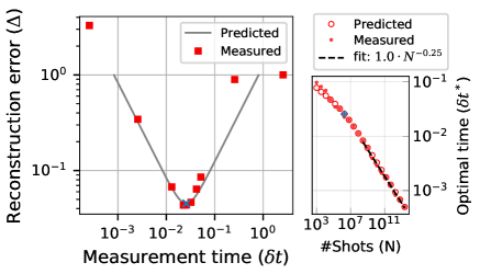
Figure 1: Tradeoff between statistical and systematic errors determines optimal measurement time. Left: reconstruction error $\Delta$ [Eq. (9)] of a random $2$-ranged Hamiltonian as a function of the measurement time $\delta t$ for a fixed measurement budget $N=10^{6}$. While the statistical error in the finite difference method decreases with $\delta t$, the systematic error increases with $\delta t$, dictating an optimal measurement time. A prior estimate of the reconstruction error (gray line), calculated using a noisy guess of the Hamiltonian [Eq. (15)], predicts the optimal time (blue ’x’). Time is measured in units of the variance of the Hamiltonain couplings [see Eq. (8)]. Right: optimal measurement time $\delta t^{*}$ as a function of the number of shots $N$ (dots measured, circles predicted). The dashed line is a fit to the asymptotic scaling $\delta t^{*}\sim N^{-\gamma}$ with $\gamma={1/4}$. The reported values average over 10 different realizations of the statistical estimation error for the observables; errorbars are smaller than the markers.

The accuracy of the Hamiltonian reconstruction from Eq. (5) is determined by the estimation accuracy of $\vec{b}$. In any experiment, instead of the exact $\vec{b}$ we can only obtain a noisy estimate $\vec{b}+\delta\vec{b}$. The estimation error $\delta\vec{b}$ corrupts the recovered coefficients, given by $\vec{c}+\delta\vec{c}=K^{+}\left(\vec{b}+\delta\vec{b}\right)$. This leads to an error in the reconstructed Hamiltonian, such that the deviation between the true and the recovered coefficients is given by $\delta\vec{c}=K^{+}\delta\vec{b}$.

The error $\delta\vec{b}$ in estimating the time-derivatives from Eq. (6) arises due to two factors: the finite measurement budget (number of experimental shots) and the finite-time approximation of the derivative. The finite sampling of $\frac{\expectationvalue{A(\delta t)}}{\delta t}$ leads to statistical error which decreases with the number of experiments and measurement time, $\norm{\delta\vec{b}_{stat}}\sim\frac{1}{\sqrt{N}\delta t}$ (for a fixed $N_{spam}$). The finite-time approximation of the derivative leads to a systematic error which increases with time, $\norm{\delta\vec{b}_{sys}}\sim\delta t$. The optimal measurement time is determined by a tradeoff between those two factors. The total estimation error $\delta\vec{b}=\delta\vec{b}_{stat}+\delta\vec{b}_{sys}$ is minimized when they are both of comparable magnitude $\frac{1}{\sqrt{N}\delta t}\sim\delta t$, which occurs at an optimal measurement time scaling with the number of experiments as $\delta t^{*}\sim N^{-\nicefrac{{1}}{{4}}}$.

The $N^{-\nicefrac{{1}}{{4}}}$ scaling can be undertstood intuitively as follows. To achieve a reconstruction which is twice more accurate, the total estimation error must be reduced by a factor of $2$. This requires measuring at a time shorter by a factor of $2$; however, to reduce the statistical error $\norm{\delta\vec{b}_{stat}}\sim\frac{1}{\sqrt{N}\delta t}$ by a factor of $2$ at this twice shorter measurement time, the measurements must be $4$ times more accurate, which requires a number of shots $16$ times larger.

To estimate the optimal $\delta t^{*}$ more accurately, we analyze in Appendix A the contributions of the statistical and systematic errors to the reconstruction error,

$$\norm{\delta\vec{c}}=\norm{K^{+}\left(\delta\vec{b}_{stat}+\delta\vec{b}_{sys}\right)}.$$ (10)

Since the statistical error averages to zero, we find that these contributions factorize, and to leading order in $\delta t$,

$$\begin{split}\mathbb{E}\norm{\delta\vec{c}}^{2}&=\mathbb{E}\norm{K^{+}\delta\vec{b}_{stat}}^{2}+\norm{K^{+}\delta\vec{b}_{sys}}^{2}\\ &\approx\frac{a_{stat}}{N(\delta t)^{2}}+a_{sys}(\delta t)^{2},\end{split}$$ (11)

for suitable constants $a_{stat}$ and $a_{sys}$. The optimal time $\delta t^{*}$, and the corresponding optimal reconstruction error $\Delta^{*}$ are therefore approximated by

$$\delta t^{*}\approx\left(\frac{a_{stat}}{a_{sys}N}\right)^{\frac{1}{4}},\hskip 14.22636pt\Delta^{*}\approx\left(4\frac{a_{stat}a_{sys}}{N}\right)^{\frac{1}{4}}/\norm{\vec{c}}.$$ (12)

The statistical component $a_{stat}$ determines how finite sampling errors degrade the reconstruction. We find that it is given by the spectrum of $\frac{1}{\sqrt{N_{spam}}}K$, which quantifies the sensitivity of the SPAM settings to all the Hamiltonian parameters, averaged over the $N_{spam}$ SPAM settings,

$$a_{stat}=\Tr\left(\left(\frac{1}{N_{spam}}K^{T}K\right)^{-1}\right).$$ (13)

The systematic compenent of the error stems from the higher-order derivatives of the estimated observables. When the systematic error is calculated to leading order in $\delta t$, it is given by

$$a_{sys}=\norm{K^{+}\partial_{tt}\expectationvalue{\vec{A}}|_{t=0}}^{2},$$ (14)

where $\partial_{tt}\expectationvalue{A}=-\expectationvalue{\left[H,\left[H,A\right]\right]}$. A more accurate estimate for long times (small $N$) can be calculated using higher orders derivatives (e.g. using $\partial_{ttt}\expectationvalue{A}$ as well, see Appendix A.2). Since the systematic error depends on the unknown Hamiltonian we wish to reconstruct, it must be estimated separately; for instance, by computing it with respect to a guess of the true Hamiltonian.

Remarkably, a rough guess of the true Hamiltonian provides an excellent estimate for the reconstruction error and optimal measurement time. We estimated these quantities for the experiments presented in Fig. 1, using the second-order estimate for the systematic error $a_{sys}$ described in Appendix A.2. We assumed that the true Hamiltonian is known to an accuracy of $10\%$, and estimated $a_{sys}$ according to a perturbed version of the true Hamiltonian

$$H+H^{\prime}=\sum_{j}c_{j}(1+e_{j})S_{j},$$ (15)

where $e_{j}\sim N(0,{0.1}^{2})$. Plugged in Eq. (12), this estimate reproduced the reconstruction error in Fig. 1 near its optimum to an excellent accuracy (Fig. 1, left, gray line). The predicted optimal measurement time matched the empirical optimum even at moderate measurement budgets $N$. While it is tempting to improve the reconstruction using higher order finite difference methods [45], our experiments found an advantage for these methods only at impractical measurement budgets $N\geq 10^{11}$ (see Appendix A.3).

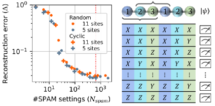
Figure 2: Left: Reconstruction error as a function of the number of different state preparation and measurement (SPAM) settings for various system sizes and a fixed total number of shots ($N=8\cdot 10^{6}$). The reconstruction accuracy of both random SPAM settings (circles) and cyclic SPAM settings (crosses) does not depend on system size, and saturates with sufficiently many settings. The saturation point is predicted by the number of settings $N_{spam}^{*}=6^{3}\cdot 3$ in the full set of cyclic settings (vertical dotted line); for $N_{spam}<N_{spam}^{*}$, the crosses correspond to random subsets of this set. Right: the measurements of the cyclic protocol (Overlapping Local Tomography) for the case of $k_{\beta}=3$-ranged observables. Partition the lattice to unit cells of length $k_{\beta}$, then measure each unit cell in an informationally complete set of bases ($3^{k_{\beta}}$ in one dimension) to obtain its reduced density matrix, repeating the bases periodically across unit cells. The reduced density matrices of overlapping partitions (gray braces) are obtained for free, since the measurement bases of the different partitions are equal up to a permutation. Initial states in the cyclic SPAM scheme are chosen similarly.

System size scaling.

So far, we numerically estimated the reconstruction error at a fixed number of SPAM settings $N_{spam}=648$ and system size $n=7$. How many SPAM settings $N_{spam}$ are required for reconstruction, and how does the measurement budget $N$ required for reconstruction scale with system size?

We repeated the reconstruction experiment of random $2$-ranged Hamiltonians [Eq. (8)] with varying numbers of different SPAM settings $N_{spam}$ and a constant total budget of measurements $N$. The reconstruction error saturated at $N_{spam}^{*}\approx 10^{3}$ SPAM settings (Fig. 2, left, dots). Crucially, both $N_{spam}^{*}$ and the reconstruction error remained unchanged when we increased the system size from $n=5$ to $n=11$, keeping the total measurement budget fixed. The larger system yielded the same reconstruction error, saturating at the same number of SPAM settings.

To understand the saturation of the reconstruction error as a function of the number of SPAM settings $N_{spam}$, we consider the $N_{spam}\rightarrow\infty$ limit of all SPAM settings. Averaging over all product states and measurement bases, the correlation matrix $\frac{1}{N_{spam}}K^{T}K$ converges to a diagonal matrix with system size independent entries (see Appendix B). The entry for each Hamiltonian term depends only on its support and on the set of measured observables. For example, if only single-site observables $A_{\beta}$ are used,

$$\frac{1}{N_{spam}}\left(K^{T}K\right)_{j,j^{\prime}}\underset{p\rightarrow\infty}{\rightarrow}4\cdot\frac{2k_{j}}{3^{k_{j}+1}}\delta_{j,j^{\prime}},$$ (16)

where $k_{j}$ is the weight of the corresponding Hamiltonian term $S_{j}$, which is the size of its support.

The insensitivity of the reconstruction to system size is apparent in the $N_{spam}\rightarrow\infty$ average over SPAM settings [Eq. (16)]. The system-size independence of the correlation matrix entries implies a system-size independent statistical error [Eq. (13)] per Hamiltonian term, as the average singular value of $K$ becomes constant. The systematic error [Eq. (14)] per Hamiltonian term is also constant for short-ranged Hamiltonians, since each Hamiltonian term affects a fixed number of observables.

More generally, the system-size independence follows from the local structure of the reconstruction algorithm, since the equations for each Hamiltonian term involve only observables in its vicinity [43]. This local structure also implies that the $N_{spam}\rightarrow\infty$ limit of Eq. (16) does not require all SPAM settings; only the local configuration of each initial state and measurement basis matters. To predict the number of SPAM configurations required to saturate the reconstruction error, we now devise a structured SPAM scheme. This structured scheme uses a finite number of ’cyclic’ SPAM configurations which are equivalent to the $N_{spam}\rightarrow\infty$ average over all configurations.

The cyclic measurement bases of the structured scheme are chosen to estimate all observables of a constant range $k_{\beta}$ in a given initial state. We construct these measurement by partitioning the lattice to unit cells of length $k_{\beta}$, and iterating over all measurement configurations within a unit cell (Fig. 2, right). The configurations are copied between unit cells, defining a set of $3^{k_{\beta}}$ measurement bases in one dimension, or $3^{k_{\beta}^{D}}$ bases in a $D$-dimensional lattice, independent of system size. Inspired by Ref. [51], we call this measurement process ’Overlapping local tomography’, since it characterizes all the $k_{\beta}$-ranged reduced density matrices of a given state.

The cyclic initial states are constructed similarly to the cyclic measurement bases. For the purposes of reconstructing a $k$-ranged Hamiltonian, cyclic initial states with periodicity $2k-1$ are equivalent to the full set of initial product states. This periodicity is chosen to uniformly cover the shared support of every pair of overlapping Hamiltonian terms $S_{i}$, $S_{j}$ (see Appendix B). For the $k=2$-ranged Hamiltonians and $1$-ranged observables considered so far, this structured scheme consists of $N_{spam}^{*}=648=6^{3}\cdot 3$ configurations, corresponding to the saturation point of Fig. 2. These structured configurations yield a similar reconstruction accuracy as the random configurations (Fig. 2, left, crosses).

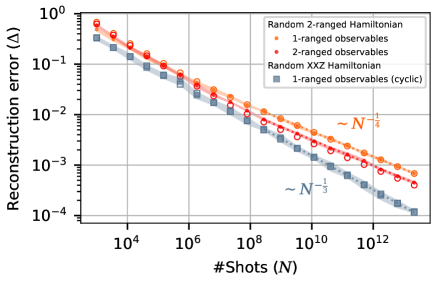
Figure 3: Reconstruction error as a function of the total number of shots. Warm colors: reconstruction of random $2$-ranged Hamiltonians using all observables up to range $k_{\beta}=1$ (orange) and $k_{\beta}=2$ (red). Addition of $2$-ranged observables improves the reconstruction accuracy at the same measurement budget $N$. Blue: reconstruction of random XXZ Hamiltonians using $1$-ranged observables in a cyclic measurement scheme with periodicity $2$. Symmetries of the XXZ model lead to an easier reconstruction, with error scaling asymptotically as $N^{-1/3}$ in contrast to the $N^{-1/4}$ scaling predicted for generic Hamiltonians.

Choosing the observables.

An important factor in the reconstruction is the choice of observables ${\{A_{\beta}\}}$ used for building the linear equation Eq. (5). Each measurement setting can be used to estimate $2^{n}-1$ commuting Pauli observables. Our previous simulations used only single-site observables in the reconstruction. How does the choice of estimated observables affect the reconstruction quality?

To test this, we repeated our simulations with different choices of observables. We used a fixed dataset of experimental outcomes to estimate all observables up to range $k_{\beta}$ for $k_{\beta}=1,2,3$. While reconstruction with $k_{\beta}=1$ observables was improved by the addition of $k_{\beta}=2$ observables (Fig. 3, warm colors), the addition of $k_{\beta}=3$ degraded the reconstruction (not shown). Correlations between estimated observables cause the degradation for $k_{\beta}=3$, as well as the deviation between predicted and measured errors for $k_{\beta}=2$ (see Appendix A.1); we conjecture that observables up to a range matching that of the Hamiltonian $k_{\beta}=k$ are optimal more generally.

Symmetry eases Hamiltonian reconstruction.

In contrast to the Hamiltonians we simulated so far, realistic Hamiltonians are not fully random and often have symmetries. How does symmetry affect the reconstruction quality and the accuracy of the our predictions?

To address this question, we repeated our experiments with random XXZ Hamiltonians:

$$H_{XXZ}=\sum_{i=0}^{n-1}c_{i}Z_{i}Z_{i+1}+a_{i}(X_{i}X_{i+1}+Y_{i}Y_{i+1}),$$ (17)

where $c_{i},a_{i}\sim N(0,1)$ are drawn from a Gaussian distribution. These $XXZ$ Hamiltonians are invariant under three anti-unitary symmetries $\forall i:\sigma_{i}^{\alpha}\mapsto-\sigma_{i}^{\alpha}$, each of which flips one of the Bloch axes $\alpha$ for all spins $i$ [54]. Interestingly, the reconstruction error of these Hamiltonians in a cyclic measurement scheme decreased more rapidly with the total number of shots $\Delta\sim N^{-1/3}$ compared to the naive prediction $N^{-1/4}$ of Eq. (12) (Fig. 3, blue). We find that for initial states that respect at least one of the anti-unitary symmetries of the Hamiltonian, the systematic error $a_{sys}$ [Eq. (14)] vanishes to first order (see Appendix C). As a result, the systematic error scales as $\norm{\delta\vec{b}_{sys}}\sim\order{\delta t^{2}}$ instead of $\order{dt}$, explaining the $N^{-1/3}$ scaling of the reconstruction error.

Conclusions.

We have shown that a system-size independent number of short-time measurements fully characterizes short-ranged Hamiltonians to any given accuracy. Fixing the total number of experimental shots, the error decreases with the number of experimental configurations up to a saturation point. While the error is very sensitive to the measurement time, the optimal time can be predicted using minimal prior knowledge.

Short-time measurements for Hamiltonian reconstruction benefit from computational and analytical tractability, as well as favorable system-size scaling. However, the reconstruction scales poorly with the number of shots, since the derivative estimation requires evolution times which decrease with the desired reconstruction accuracy. Longer measurement times can be utilized by substituting the differential Ehrenfest equation [Eq. (2)] by an integral equation for the dynamics of observables over a time period. Altenatively, a higher-order Taylor expansion of the observable dynamics would lead to a non-linear set of equations, allowing longer measurement times at the cost of higher computational effort as in the recent Ref. [55]. The optimal measurement time for these higher order methods can be estimated using extensions of the method we presented here.

Alternatively, recent works discuss a scheme for dynamical Hamiltonian learning which is based on on energy conservation [56, 48]. These works look for a local observable which does not change with time. In the absence of other local symmetries, the only conserved observable is the Hamiltonian. Thus, each initial state or measurement time gives a single linear equation for the Hamiltonian, such that $\order{n}$ suffice to uniquely identify it. The equations remain computationally tractable for long evolution times, increasing their sensitivity at a fixed system size. In our short-time approach, each measurement settings yields not one but $\order{n}$ local equations for the Hamiltonian, providing an advantage at large system sizes.

Appendix A Derivative estimation

A.1 Full derivation of the optimal measurement time

A.1.1 Full derivation of $\mathbb{E}\norm{\delta\vec{c}}$ bound

We want to estimate how $\delta t$ affects $\mathbb{E}\norm{\delta\vec{c}}$. The effect of $\delta t$ on $\delta\vec{b}$ can be written as sum of two contributions $\delta\vec{b}=\delta\vec{b}_{sys}+\delta\vec{b}_{stat}$ where

$$\delta b_{sys_{\left(\alpha,\beta\right)}}=b_{\left(\alpha,\beta\right)}-\frac{\expectationvalue{A_{\beta}}_{\psi_{\alpha}(\delta t)}-\expectationvalue{A_{\beta}}_{\psi_{\alpha}(0)}}{\delta t},\$$ (18)

with expectation values evaluated exactly (in the limit of infinite shots), is the systematic error of the estimation (Eq. (6)) and

$$\delta b_{stat_{\left(\alpha,\beta\right)}}=\frac{\delta\expectationvalue{A_{\beta}}_{\psi_{\alpha}(\delta t)}}{\delta t}\sim G\left(0,\frac{1}{{\delta t}^{2}}\frac{N_{spam}}{N}\right),$$ (19)

with expectation values estimated using $\frac{N}{N_{spam}}$ shots, is the statistical error due to finite sampling. Writing $\delta\vec{c}=K^{+}\delta\vec{b}=K^{+}\left(\delta\vec{b}_{stat}+\delta\vec{b}_{sys}\right)$ as sum of two independent errors allows us to find a value for $\mathbb{E}\norm{\delta\vec{c}}^{2}$ using the following lemma on the expectation value of a quadratic form.

Lemma A.1.

Let $\vec{x}$ be a random vector with mean $\vec{\mu}$ and covariance matrix $\Sigma$ then for any $A\in M_{n,m}(\mathbb{R})$, $\mathbb{E}\norm{A\vec{x}}^{2}=\Tr\left(\Sigma A^{T}A\right)+\norm{A\vec{\mu}}^{2}$.

Proof.

Note that

$$\norm{A\vec{x}}^{2}=\vec{x}^{T}A^{T}A\vec{x}$$

Because $\norm{A\vec{x}}$ is a scalar, we can write

$$\norm{A\vec{x}}^{2}=\Tr\left(\vec{x}^{T}A^{T}A\vec{x}\right)$$

Using the cyclic property of the trace

$$\norm{A\vec{x}}^{2}=\Tr\left(A^{T}A\vec{x}\vec{x}^{T}\right)$$

As trace and matrix multiplication are essentially additions and scalar multiplications we can write

$$\mathbb{E}\Tr\left(A^{T}A\vec{x}\vec{x}^{T}\right)=\Tr\left(A^{T}A\mathbb{E}\left(\vec{x}\vec{x}^{T}\right)\right)$$

Using the definition of the covariance matrix

$$\mathbb{E}\norm{A\vec{x}}^{2}=\Tr\left(A^{T}A\left(\Sigma+\vec{\mu}\vec{\mu}^{T}\right)\right)$$

and from linearity of the trace

$$\mathbb{E}\norm{A\vec{x}}^{2}=Tr\left(A^{T}A\Sigma\right)+\Tr\left(A^{T}A\vec{\mu}\vec{\mu}^{T}\right)$$

Again from the cyclic properties of the trace and the fact that $\Tr\left(\vec{\mu}^{T}A^{T}A\vec{\mu}\right)=\norm{A\vec{\mu}}^{2}$ (as it is a scalar):

$$\mathbb{E}\norm{A\vec{x}}^{2}=\Tr\left(\Sigma A^{T}A\right)+\norm{A\vec{\mu}}^{2}$$

∎

In our case $\delta\vec{b}$ is a random vector with mean $\delta\vec{b}_{sys}$ and covariance matrix $\Sigma_{\delta\vec{b}_{stat}}=\mathbb{E}\delta\vec{b}_{stat}\delta\vec{b}_{stat}^{T}$. Using that lemma for $\mathbb{E}\norm{\delta\vec{c}}^{2}=\mathbb{E}\norm{K^{+}\delta\vec{b}}^{2}$ we can find a bound on $\mathbb{E}\norm{\delta\vec{c}}$ using Jensen inequality $\mathbb{E}\norm{\delta\vec{c}}\leq\sqrt{\mathbb{E}\norm{\delta\vec{c}}^{2}}$:

$$\mathbb{E}\norm{\delta\vec{c}}\leq\sqrt{\Tr\left(\mathbb{E}\left(\delta\vec{b}_{stat}{\delta\vec{b}_{stat}}^{T}\right){K^{+}}^{T}K^{+}\right)+\norm{K^{+}\delta\vec{b}_{sys}}^{2}}.$$

Assuming each entry of $\delta\vec{b}_{stat}$ is independent random variable with variance $\sigma_{(\alpha,\beta)}^{2}$ and zero mean we get that

$$\mathbb{E}\norm{\delta\vec{c}}\leq\sqrt{\Tr\left(\Sigma_{\delta\vec{b}_{stat}}{K^{+}}^{T}K^{+}\right)+\norm{K^{+}\delta\vec{b}_{sys}}^{2}},$$ (20)

where $\Sigma_{\delta\vec{b}_{stat}}$ is diagonal with elements $\sigma_{(\alpha,\beta)}^{2}$. Assuming $\sigma_{(\alpha,\beta)}\sim\left(\frac{N}{N_{spam}}\right)^{-\nicefrac{{1}}{{2}}}\frac{1}{\delta t}$ we can define

$${a}_{stat}=\Tr\left(\Sigma_{\delta\vec{b}_{stat}}^{*}N_{spam}{K^{+}}^{T}K^{+}\right)$$

where $\Sigma_{\delta\vec{b}_{stat}}^{*}=\frac{N}{N_{spam}}{\delta t}^{2}\Sigma_{\delta\vec{b}_{stat}}$ is a diagonal matrix which is independent of $N,p,\delta t$ and

$$a_{sys}=\frac{1}{{\delta t}^{2}}\norm{K^{+}\delta\vec{b}_{sys}}^{2}$$

Assuming $\delta\vec{b}_{sys}\sim\delta t$ (first order estimation of the systematic error) we get Eq. (11), and if we assume that $\Sigma_{\delta\vec{b}_{stat}}^{*}=\mathbb{1}$ (i.e. all the observables have the same statistical error magnitude) using the cyclic property of the trace we can write ${a}_{stat}=\Tr\left(N_{spam}\left(K^{T}K\right)^{-1}\right)$.

In practice, the standard deviations varies between observables depending on the initial state. Moreover, when different observables are estimated from the same set of measurements, off-diagonal entries appear in the covariance matrix. These correlations explain the deviation between the predicted and observed accuracies in Fig. 3. They can be taken into account in order to improve the prediction of the reconstruction, and to predict the optimal set of estimated observables.

A.1.2 Estimating the optimal $\delta t$

In Eq. (11) and subsequent derivations, we have assumed that the statistical error scales as $\delta\vec{b}_{stat}\propto{\left(\frac{N}{N_{spam}}\right)}^{-\nicefrac{{1}}{{2}}}\delta t^{-1}$ and the systematic error as $\delta\vec{b}_{sys}\propto\delta t$. We can examine a more general case with

$$\delta\vec{b}_{stat}=\vec{a}_{stat}{\left(\frac{N}{N_{spam}}\right)}^{-\nicefrac{{1}}{{2}}}{\delta t}^{-\gamma}$$

$$\delta\vec{b}_{sys}=\vec{a}_{sys}{\delta t}^{\lambda}+\order{\delta t^{\lambda+1}}$$

for $\lambda,\gamma\neq 1$. $\vec{a}_{stat},\vec{a}_{sys}$ are defined such that they are independent of $\delta t$. The optimal $\delta t$ is achieved when $\mathbb{E}\norm{\delta\vec{c}}$ is minimal. As an approximation, we use the bound $\norm{\delta c}_{bound}=\sqrt{\Tr\left(\Sigma_{\delta\vec{b}_{stat}}{K^{+}}^{T}K^{+}\right)+\norm{K^{+}\delta\vec{b}_{sys}}^{2}}$ of Eq. (20), and minimize it with respect to $\delta t$. To leading order in $\delta t$ we get

$$\norm{\delta c}_{bound}^{2}=\frac{{\delta t}^{-2\gamma}}{N}\Tr\left(\Sigma_{\vec{a}_{stat}}{K^{+}}^{T}K^{+}\right)\\ +{\delta t}^{2\lambda}\norm{K^{+}\delta\vec{a}_{sys}}^{2}.$$

The derivative is given by

$$\dfrac{d}{d(\delta t)}\norm{\delta c}_{bound}^{2}=-2\frac{\gamma{\delta t}^{-2\gamma-1}}{N}\Tr\left(\Sigma_{\vec{a}_{stat}}{K^{+}}^{T}K^{+}\right)\\ +2\lambda{\delta t}^{2\lambda-1}\norm{K^{+}\delta\vec{a}_{sys}}^{2}$$

The minimum is achieved when the derivative vanishes, which occurs at

$$\delta t^{*}=\left(\frac{1}{N}\cdot\frac{\gamma\Tr\left(\Sigma_{\vec{a}_{stat}}{K^{+}}^{T}K^{+}\right)}{\lambda\norm{K^{+}\delta\vec{a}_{sys}}^{2}}\right)^{\nicefrac{{1}}{{2\left(\gamma+\lambda\right)}}},$$ (21)

which corresponds to reconstruction error

$$\norm{\delta c^{*}}_{bound}=\left(\sqrt{\frac{1}{1-\kappa}}\frac{1}{\sqrt{N}}\sqrt{\Tr\left(\Sigma_{\vec{a}_{stat}}{K^{+}}^{T}K^{+}\right)}\right)^{1-\kappa}\\ \cdot\left(\sqrt{\frac{1}{\kappa}}\norm{K^{+}\delta\vec{a}_{sys}}\right)^{\kappa},$$ (22)

where $\kappa=\frac{\gamma}{\lambda+\gamma}$. This result generalizes Eq. (12), where $\gamma=\lambda=1$ and $\kappa=\nicefrac{{1}}{{2}}$.

A.2 Estimation used in the Hamiltonian reconstruction simulations

In our simulations, the systematic error due to the finite derivative method was estimated using a perturbed version of the real Hamiltonian, used to calculate the higher derivatives $\partial_{tt}\expectationvalue{A_{j}}_{t=0}$ and $\partial_{ttt}\expectationvalue{A_{j}}_{t=0}$ of the observables. The systematic error is defined as

$$a_{sys}=\norm{K^{+}\left(\partial_{t}\expectationvalue{\vec{A}}|_{t=0}-\frac{\expectationvalue{\vec{A}}_{\delta t}-\expectationvalue{\vec{A}}_{0}}{\delta t}\right)}^{2}.$$

Writing $\expectationvalue{\vec{A}}_{\delta t}$ as a Taylor expansion around $t=0$ gives:

$$\expectationvalue{\vec{A}}_{\delta t}=\expectationvalue{\vec{A}}_{0}+\delta t\partial_{t}\expectationvalue{\vec{A}}|_{0}+\frac{{\delta t}^{2}}{2}\partial_{tt}\expectationvalue{\vec{A}}|_{0}\\ +\frac{{\delta t}^{3}}{6}\partial_{ttt}\expectationvalue{\vec{A}}|_{0}+\order{{\delta t}^{4}}$$ (23)

Then for first order in $\delta t$ the systematic error is:

$$a_{sys}=\norm{K^{+}\left(\frac{1}{2}\partial_{tt}\expectationvalue{\vec{A}}|_{t=0}\right)}^{2}$$

and for second order in $\delta t$:

$$a_{sys}=\norm{K^{+}\left(\frac{1}{2}\partial_{tt}\expectationvalue{\vec{A}}|_{t=0}+\frac{\delta t}{6}\partial_{ttt}\expectationvalue{\vec{A}}|_{t=0}\right)}^{2}$$ (24)

Evaluating this second order estimate for $a_{sys}$ requires to know $\delta t$ which is our ultimate goal to find. In order to bypass this difficulty, we used the first order estimate of $a_{sys}$ in Eq. (12) to get a first order estimate of $\delta t$, and used that estimate in the second order estimate of $a_{sys}$ to get a better prediction of $\delta t$.

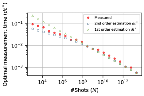
Figure S4: Predicting the optimal measurement time using first order (green hollow triangles, Eq. (14)) or second order (blue circles, Eq. (24)) methods in a random 2-local Hamiltonian compared to the measured optimal time (red dots). Here we used $2$-ranged observables in a randomized measurement scheme.

A.3 Higher order finite difference approximations

Examining the analytical results we got for the reconstruction error bound in Eq. (22) we can try to improve the reconstruction using higher-order estimates for the derivative. Instead of using the finite difference method with a single forward point (Eq. (6)), we can use forward finite difference method with $\lambda>1$ points

$$\partial_{t}\expectationvalue{A}_{\psi}=\frac{\sum_{r=0}^{\lambda}w_{r}\expectationvalue{A}_{\psi(r\cdot\delta t)}}{\delta t}+\order{\delta t^{\lambda}}$$ (25)

where $w_{r}$ are the weights of each point such that the estimation error is $\order{\delta t^{\lambda}}$. In that case we will achieve better asymptotic behaviour with respect to the number of measurements (as $\norm{\delta c^{*}}_{bound}\propto\sqrt{N}^{\frac{\lambda}{\lambda+1}}$, Eq. (22)) but the measurement budget will split between $\lambda$ measurement times. The measurement budget at different times can allocated wisely by finding a set $\{N_{r}\}_{r=1}^{\lambda};\sum_{r=1}^{\lambda}N_{r}=N$ which minimizes the variance of the statistical error $\sigma^{2}=\sum_{r=1}^{\lambda}{w_{r}}^{2}/{N_{r}}$, which is achieved for

$$N_{r}=N\frac{\absolutevalue{w_{r}}}{\sum_{r=1}^{\lambda}\absolutevalue{w_{r}}}.$$ (26)

Hence, the $N$ used in the statistical error should be replaced with $N_{effective}=N\left(\frac{1}{\sum_{r=1}^{\lambda}\absolutevalue{w_{r}}}\right)^{2}$, which yields an additional $\left(\sum_{r=1}^{\lambda}\absolutevalue{w_{r}}\right)^{\frac{\lambda}{\lambda+1}}$ factor to the reconstruction error bound because of the statistical error (Eq. (22)). Additional factors can arise due to the systematic error.

We examined the results of reconstruction using finite difference with $\lambda=2$ uniformly spaced forward points

$$\partial_{t}\expectationvalue{A}_{\psi}=\frac{-\frac{3}{2}\expectationvalue{A}_{\psi(0)}+2\expectationvalue{A}_{\psi(\delta t)}-\frac{1}{2}\expectationvalue{A}_{\psi(2\delta t)}}{\delta t}+\order{\delta t^{2}}.$$ (27)

Comparing the results we got using 1 forward point finite difference (Eq. (6)) to the results using 2 forward points finite difference (Eq. (27)) we observed that the scaling advantage from the the 2 forward points estimation method yields better reconstruction only for $N>10^{11}$ as can be seen in Fig. S5.

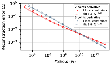
Figure S5: Reconstruction error of a random 2-local Hamiltonian as a function of the total number of shots using different methods of derivative estimation: 2 points forward finite difference (blue dots, Eq. (6)) and 3 points forward finite difference (red dots, Eq. (27)).

Appendix B Analytic estimate of the statistical reconstruction error

A unique reconstruction requires a set of initial states and measurement bases leading to a full rank reconstruction matrix $K$. More generally, the choice of experiments determines the spectrum of $K^{T}K$, which quantifies the sensitivity of the experiments to the Hamiltonian terms through the statistical error of Eq. (13). We now derive the analytical form of $K^{T}K$ when averaged over all experimental configurations, and show that it is sufficient to average over a finite set of local configurations.

For a given set of initial states $\ket{\psi_{\alpha}}$ and observables $A_{\beta}$,

$$(K^{T}K)_{ij}=-\sum_{\alpha,\beta}\expectationvalue{i[S_{i},A_{\beta}]}_{\psi_{\alpha}}\expectationvalue{i[S_{j},A_{\beta}]}_{\psi_{\alpha}},$$ (28)

by the definition of $K$ [Eq. (3)]. Here, $A_{\beta}$ denote all the observables compatible with the measurement basis for the initial state $\ket{\psi_{\alpha}}$ up to the chosen locality. When averaging over all possible configurations, each of the $6^{n}$ initial states is measured in $3^{n}$ measurement bases. However, for a given initial state $\ket{\psi_{\alpha}}$, each observable $A_{\beta}$ is compatible with many measurement bases. An observable with support $s\subseteq[1,\dots,n]$ is compatible with $\frac{1}{3^{\absolutevalue{s}}}$ of all measurement bases; for instance, $X_{1}$ is compatible with $\frac{1}{3}$ of all bases. Therefore, the average $\frac{1}{N_{spam}}(K^{T}K)_{ij}$ over all configurations $N_{spam}=\frac{1}{3^{n}\cdot 6^{n}}$ takes the form

$$\sum_{\beta}\frac{1}{3^{\absolutevalue{s_{\beta}}}}\sum_{\alpha}\frac{1}{6^{n}}\expectationvalue{i[S_{i},A_{\beta}]}_{\psi_{\alpha}}\expectationvalue{i[S_{j},A_{\beta}]}_{\psi_{\alpha}}.$$ (29)

where $\beta$ runs over all estimated observables. We will now show that this average

1. Vanishes for off-diagonal elements where $S_{i}\neq S_{j}$.

2. For the diagonal element corresponding to $S_{i}$, it counts the number of observables $A_{\beta}$ that fail to commute with $S_{i}$, normalized by the weight $s_{\beta}$ of $A_{\beta}$ and the weight ${s_{i,\beta}}$ of the commutator $\left[S_{i},A_{\beta}\right]$.

3. Depends only on initial state and measurement configurations on sites supported by $S_{i}$ or $S_{j}$.

4. Vanishes identically for any initial state $\ket{\psi_{\alpha}}$ when $S_{i},S_{j}$ do not overlap at least on one site, so that averaging over $2k_{h}-1$-local configurations suffices.

For the first two claims, we invoke the following formula for product state averages of Pauli strings [48]:

$$\frac{1}{6^{n}}\sum_{\alpha}\expectationvalue{P_{r}}_{\psi_{\alpha}}\expectationvalue{P_{r}^{\prime}}_{\psi_{\alpha}}=\frac{1}{3^{\absolutevalue{s_{r}}}}\delta_{r,r^{\prime}},$$ (30)

which states that the average over all initial states vanishes whenever the two Pauli strings are different, and decays with their support $\absolutevalue{s_{r}}$ otherwise. In our case, $i\left[S_{i},A_{\beta}\right]=2P_{r_{i,\beta}}$ is a Pauli string since both $S_{i}$ and $A_{\beta}$ are.

Off-diagonal terms vanish.

Considering Eq. (30), it is sufficient to show that different Hamiltonian terms $S_{i}\neq S_{j}$ have different commutators with a shared Pauli observable $[S_{i},A_{\beta}]\neq[S_{j},A_{\beta}]$, assuming that both commutators are non-zero. To see this, we recall that any pair of Paulis either commutes or anticommutes. Therefore, if $\left[S_{i},A_{\beta}\right]\neq 0$, we can write $\left[S_{i},A_{\beta}\right]=\theta_{i,\beta}S_{i}A_{\beta}$ for some $\theta_{i,\beta}\neq 0$, and similarly for $S_{j}$. If $\left[S_{i},A_{\beta}\right]=\left[S_{j},A_{\beta}\right]$, then $\theta_{i,\beta}S_{i}A_{\beta}=\theta_{j,\beta}S_{j}A_{\beta}$, and $S_{i}=\theta_{i,\beta}^{-1}\theta_{j,\beta}S_{j}$, in contradiction to our assumption.

Diagonal elements count non-commuting observables.

For diagonal elements $i=j$, Eq. (30) gives a positive contribution whenever $\left[S_{i},A_{\beta}\right]\neq 0$. The average over initial states $\alpha$ yields a contribution $\frac{4}{3^{\absolutevalue{s_{i,\beta}}}}$ which depends only on the size of the support $s_{i,\beta}$ of the commutator $\left[S_{i},A_{\beta}\right]$, such that Eq. (29) becomes

$$\sum_{A_{\beta}:\left[S_{i},A_{\beta}\right]\neq 0}\frac{4}{3^{\absolutevalue{s_{\beta}}+\absolutevalue{s_{i,\beta}}}},$$ (31)

where the sum runs over all observables $A_{\beta}$ up to the chosen observable locality that fail to commute with $S_{i}$, and the factor 4 comes from the two commutators. For example, for single-site $S_{i}$ and $A_{\beta}$ we get $4\cdot\frac{2}{9}$, since $\frac{2}{3}$ of all single-site Paulis $A_{\beta}$ fail some commute with a single-site Hamiltonian Pauli $S_{i}$; and $\frac{1}{3}$ of the Pauli measurement bases match each given commutator.

More generally, since our measurement bases average equally over all observables $A_{\beta}$ with the same support, the value of Eq. (29) depends only on the support of $S_{i}$, i.e. its locality and range. It can be calculated explicitly for a given set of estimated observables $A_{\beta}$.

Only local configurations matter.

We now show that for each $i,j$, Eq. (29) depends only on local configurations within the support of $S_{i}$ and $S_{j}$. Namely, it does not depend on the initial state configuration on sites supported by the observable $A_{\beta}$ but not by any of the Hamiltonian terms. We assume that all observables $A_{\beta}$ with a given support are sampled equally, as in the overlapping local tomography (’cyclic’) measurement scheme.

Consider a fixed initial state $\ket{\psi_{\alpha}}$, and the average over all observables $A_{\beta}$ with a given support $s$:

$$\frac{1}{3^{\absolutevalue{s}}}\sum_{A_{\beta}:\text{supp}(A_{\beta})=s}\expectationvalue{i[S_{i},A_{\beta}]}_{\psi_{\alpha}}\expectationvalue{i[S_{j},A_{\beta}]}_{\psi_{\alpha}}.$$ (32)

The Paulis of $A_{\beta}$ on the sites are untouched by $S_{i}$ or $S_{j}$ factor out of both commutators. When we average over all observables with the same support, only a single observable configuration on those sites matches the initial state $\ket{\psi_{\alpha}}$, regardless of the initial state or Hamiltonian terms. Formally, we split $A_{\beta}$ to the part that intersects $S_{i}$ or $S_{j}$ and the part that does not,

$$A_{\beta}=A_{\beta}^{s\cap s_{ij}}\cdot A_{\beta}^{s\setminus s_{ij}}=\prod_{i=1}^{\absolutevalue{s\cap s_{ij}}}\sigma_{m_{i}}^{\beta_{m_{i}}}\prod_{i=\absolutevalue{s\cap s_{ij}}+1}^{\absolutevalue{s}}\sigma_{m_{i}}^{\beta_{m_{i}}}$$ (33)

where $m$ is a site index, $\beta_{m}\in\{X,Y,Z\}$ is a Pauli index, and $s_{ij}\stackrel{{\scriptstyle\mathrm{def}}}{{=}}\text{supp}(S_{i})\cup\text{supp}(S_{j})$. We can then write Eq. (32) as

$$\frac{1}{3^{\absolutevalue{s}}}\sum_{\beta_{m_{1}},\dots,\beta_{m_{\absolutevalue{s\cap s_{ij}}}}} \expectationvalue{i[S_{i},A_{\beta}^{s\cap s_{ij}}]}_{\psi_{\alpha}}\expectationvalue{i[S_{j},A_{\beta}^{s\cap s_{ij}}]}_{\psi_{\alpha}}\cdot$$ (34)

$$\cdot\sum_{\beta_{\absolutevalue{s\cap s_{ij}}+1},\dots,\beta_{\absolutevalue{s}}}\expectationvalue{A_{\beta}^{s\setminus s_{ij}}}_{\psi_{\alpha}}^{2}.$$ (35)

For any given initial state, the second sum over all observable configurations that are untouched by $S_{i}$ or $S_{j}$ gives 1. Since the first sum depends only on the initial state configurations in $s\cap s_{ij}$, it is sufficient to average over those.

Distant off-diagonal terms vanish for any product state.

We now show that $(K^{T}K)_{ij}$ vanishes for each of our initial states whenever $S_{i},S_{j}$ do not overlap. For a given Pauli observable $A_{\beta}$, we done its part that intersects $S_{i}$ by $A_{\beta}^{s_{i}}$; namely, we partition $A_{\beta}$ to

$$A_{\beta}=A_{\beta}^{s_{i}}\cdot A_{\beta}^{s\setminus s_{i}}.$$ (36)

If $A_{\beta}$ commutes with $S_{i}$, its contribution to Eq. (29) vanishes. To have a non-vanishing contribution, it must anticommute with $S_{i}$, since Pauli strings either commute or anticommute. In this case, we must have that $A_{\beta}^{s_{i}}$ anticommutes with $S_{i}$, since $A_{\beta}^{s\setminus s_{i}}$ trivially commutes with it. However, $A_{\beta}^{s_{i}}$ commutes with $S_{j}$, since they do not overlap. Therefore, since expectation values in product states factorize,

$$\expectationvalue{i[S_{i},A_{\beta}]}_{\psi_{\alpha}}\expectationvalue{i[S_{j},A_{\beta}]}_{\psi_{\alpha}}=$$ (37)

$$=\expectationvalue{i[S_{i},A_{\beta}^{s_{i}}]}\expectationvalue{A_{\beta}^{s\setminus s_{i}}}\expectationvalue{A_{\beta}^{s_{i}}}\expectationvalue{i[S_{i},A_{\beta}^{s\setminus s_{i}}]}.$$ (38)

This product includes the expectation values of anticommuting Pauli strings: $A_{\beta}^{s_{i}}$ anticommutes with $i\left[S_{i},A_{\beta}^{s_{i}}\right]$, since we assumed it anticommutes with $S_{i}$. As our initial states are stabilizer states, their expectation value cannot be non-zero for a pair of anticommuting Pauli strings, leading to a vanishing contribution to Eq. (29) for any Pauli observable $A_{\beta}$.

$2k_{h}-1$-local configurations suffice.

We have shown that for pair of Hamiltonian terms $S_{i},S_{j}$, it is sufficient to sample local configurations on their shared support; and that it is sufficient to consider Hamiltonian terms that intersect. Therefore, $\frac{1}{N_{spam}}K^{T}K$ becomes diagonal with entries described by Eq. (31) if all the local initial state configurations are uniformly sampled within any $2k_{h}-1$-ranged patch.

B.1 Examples for diagonal entry calculations

We would like to evaluate the diagonal entries of $\frac{1}{N_{spam}}K^{T}K$ in the limit of all SPAM settings $N_{spam}\rightarrow\infty$ [Eq. (28)] for a few simple cases: (i) $1$-local observables and generic Hamiltonian terms, corresponding to the result of Eq. (16) and (ii) $1$-local Hamiltonian terms and generic observables.

The diagonal entry for a Hamiltonian term $S_{i}$ [Eq. (31)] counts the number of measured observables that do not commute with it, normalized by the weight of the observable and of the commutator. For instance, each $1$-local observable $A_{\beta}$ is compatible with one third of all measurement bases, yielding a normalization factor $\frac{1}{3}$ for the observable locality ($s_{\beta}=1$). Given a weight $k_{i}$ Hamiltonian term $S_{i}$, any non-zero commutator $[S_{i},A_{\beta}]$ is itself of weight $k_{i}$, vanishing in all but $\frac{1}{3^{k_{i}}}$ of all initial states ($s_{i,\beta}=k_{i}$). Finally, for each of the $k_{i}$ sites in the support of $S_{i}$ there are two single-site Paulis that differ from it on that site, yielding a combinatorial factor of $2k_{i}$ non-commuting observables. We conclude that

$$\frac{1}{N_{spam}}(K^{T}K)_{ii}=\\ \sum_{A_{\beta}:\left[S_{i},A_{\beta}\right]\neq 0}\frac{4}{3^{\absolutevalue{s_{\beta}}+\absolutevalue{s_{i,\beta}}}},=4\cdot\frac{2k_{i}}{3^{k_{i}+1}}.$$

As another example, we examine the case of a $1$- local Hamiltonian term $k_{i}=1$ and range $k_{\beta}$ observables in a one-dimensional chain with periodic boundary conditions. In that case ${\absolutevalue{s_{\beta}}=\absolutevalue{s_{i,\beta}}}$. For $k_{\beta}=2$-ranged observables,

$$\frac{1}{N_{spam}}(K^{T}K)_{ii}=\frac{4}{{3^{2+2}}}\cdot{2\cdot 2\cdot 3}=4\cdot\frac{4}{3^{3}}.$$ (39)

The combinatorial factor consists of three contributions: 2 possible Pauli operators that anticommute with $S_{i}$ on the site that intersects with it; 2 possible choices of a neighboring site for the observable support; and 3 possible Pauli operators on the neighboring site. Similarly, for $k_{\beta}=3$-ranged observables, $\frac{1}{N_{spam}}(K^{T}K)_{ii}=\frac{4}{3^{3+3}}\cdot{2\cdot 3\cdot 3^{2}}+\frac{4}{3^{2+2}}\cdot 2\cdot 2\cdot 3=4\cdot\frac{18}{3^{4}}$. The left term counts the observables with both range and weight 3, while the right term counts observables with range 3 and weight 2.

The Table below sums results for $\frac{1}{4p}(K^{T}K)_{ii}$ with up to range 3 observables and weight 3 Hamiltonian terms:

	1	2	3
1	$\nicefrac{{2}}{{3^{2}}}$	$\nicefrac{{4}}{{3^{3}}}$	$\nicefrac{{18}}{{3^{4}}}$
2	$\nicefrac{{4}}{{3^{3}}}$	$\nicefrac{{16}}{{3^{4}}}$	$\nicefrac{{52}}{{3^{5}}}$
3	$\nicefrac{{6}}{{3^{4}}}$	$\nicefrac{{28}}{{3^{5}}}$	$\nicefrac{{114}}{{3^{6}}}$

The first column and row are the examples calculated above. The columns denote the contribution of all the observables with exact range $k_{\beta}$ to the diagonal entry. In the rows, we consider terms acting nontrivially on each of $k_{i}$ contiguous sites, such that $k_{i}$ denotes both the weight and range of the $S_{i}$ term. This assumption is not necessary for $k_{\beta}=1$, where the result depends only on the weight of $S_{i}$.

B.2 Cyclic measurement scheme in higher-dimensional lattices

How many copies of a state $\ket{\psi}$ on a $d$-dimensional lattice do we need to measure each $k-ranged$ observable at least once? In $1D$ we defined a unit cell of length $k$. To measure all the $k-ranged$ observables, it sufficed to iterate over the $3^{k}$ Pauli bases of a single unit cell, repeating measurement bases between different unit cells. Since different unit cell partitions are equivalent up to a permutation, this process yields at least one shot of each obsrvable using exactly $3^{k}$ copies of the state.

We can generalize this approach to $d$-dimensional lattices. We choose a $d$-dimensional square unit cell of side length $k$, containing $k^{d}$ sites (see $2D$ case in Fig. S6). As in the 1D case, we evaluate all the $k-local$ observables within it using $3^{\left(k^{d}\right)}$ different copies, repeating the measurement bases between unit cells. This procedure yields at least one sample of any observable residing within length $k$ cube, even if it does not respect the original lattice partition. Similarly, since there are $6$ Pauli eigenstates per site, $6^{k^{d}}$ initial states cover all the Pauli eigenstates in each length $k$ cube.

The local measurement process we described improves upon the overlapping tomography protocol of Ref. [51] for the special case of geometrically local lattices. The protocol of Ref. [51] recovers all $k$-local observables (maximal weight $k$) without assuming any spatial structure. The protocol requires $\mathcal{O}(\log^{2}n)$ copies of a state of $n$ qudits to recover all observables of a fixed locality to a given worst-case error. Our protocol requires an $n$-independent number of copies to recover all short-ranged observables to a constant average accuracy. It effectively eliminates one $\log n$ factor, which is required in order to cover all long-ranged observables. The other $\log n$ factor stems only from the different error metric (worst-case vs. average-case).

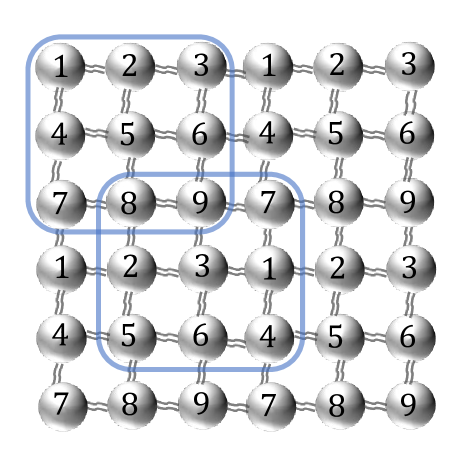
Figure S6: Example of overlapping tomography (cyclic method) in a $d=2$ dimension square lattice with $k_{\beta}=3$. The boundary of unit cells is colored in blue for two of the unit cells. In this example we need $3^{9}$ copies of $\ket{\psi}$ to get one sample of every $3$-ranged observable in the system.

Appendix C XXZ model

Why does the reconstruction error for the $XXZ$ Hamiltonians of Eq. (17) decrease more rapidly with the measurement count $\Delta\sim N^{-\nicefrac{{1}}{{3}}}$ compared to the $N^{-\nicefrac{{1}}{{4}}}$ scaling of generic $2$-local Hamiltonians?

Since the $XXZ$ Hamiltonians are real in the computational basis, they are invariant under the anti-unitary complex conjugation operator which flips $Y_{i}\mapsto-Y_{i}$ [54]. As these Hamiltonian contain only even combinations of the other Paulis $X,Z$ as well, they are actually invariant under a time-reversal symmetry for each axis $\alpha=1,2,3$ of the Bloch sphere, which flips $\sigma^{\alpha}_{i}\mapsto-\sigma^{\alpha}_{i}$.

Incidentally, each of the $2$-periodic cyclic initial states we have chosen in Fig. 3 is invariant under one of those symmetries, as the spins of each of these states are polarized only within a plane in the Bloch sphere. In other words, each of these states contains only two of the three Paulis, and is invariant under an inversion of the third. We now explain why this implies that for any Pauli observable $A$, either (i) the time derivative vanishes $\partial_{t}\expectationvalue{A}=0$, or (b) the second time-derivative vanishes $\partial_{tt}\expectationvalue{A}=0$.

Without loss of generality, we focus on the $Y\mapsto-Y$ time reversal symmetry, and consider a real-valued initial state which is invariant under the standard complex conjugation, such as $\ket{\psi}=\ket{\uparrow\uparrow\uparrow\cdots}$. Each Pauli observable $A$ has a definite parity under this symmetry: it is either real (even) or purely imaginary (odd), depending on the parity of its number of $Y$ operators. Since the Hamiltonian is real, it flips the parity of $A$ under Heisenberg evolution: if $A$ is real, then $\partial_{t}A=i\left[H,A\right]$ is imaginary and vice versa.

Importantly, if an observable $O$ and a state $\rho$ have definite time reversal parities, they must match for the observable to take an expectation value. If $\rho$ is a real density matrix and $O$ an imaginary observable, then

$$\Tr(\rho O) =\Tr((\rho O)^{T})=\Tr(\rho^{T}O^{T})$$

$$=-\Tr(O\rho)=-\Tr(\rho O),$$

since $O^{T}=(O^{\dagger})^{*}=O^{*}=-O$, and the trace of any operator is the same as the trace of its transpose.

Therefore, only time-reversal odd observables $A$ contribute to the reconstruction in a time-reversal even initial state. If $A$ is time-reversal even, then $\partial_{t}A=i\left[H,A\right]$ is time-reversal odd; in this case, $\partial_{t}\expectationvalue{A}_{\psi}$ vanishes for a time-reversal even state $\ket{\psi}$ regardless of the particular coefficients of the $XXZ$ Hamiltonian. In contrast, time-reversal odd observables $A$ have a non-trivial time derivative, since $\partial_{t}A$ is time-reversal even; however, in this case $\partial_{tt}A=-\left[H,\left[H,A\right]\right]$ is again time reversal odd, so that $\partial_{tt}\expectationvalue{A}=0$, and the systematic error [Eq. (18)] vanishes to first order in $\delta t$. Therefore, the time-reversal odd observables $A$ that participate in the reconstruction can be measured at later times compared to a generic Hamiltonian, leading to an improved scaling of the reconstruction error $N^{-\nicefrac{{1}}{{3}}}$ according to Eq. (22).

This analysis holds for every Pauli observable in a state whose spins are polarized along the $X-Z$ plane, based on the $Y\mapsto-Y$ symmetry. Since the $XXZ$ Hamiltonian is invariant under inversion of any axis of the Bloch sphere, it generalizes to any initial state whose spins are polarized along a plane. The $2$-periodic initial states satisfy this condition, explaining the findings of Fig. 3. More generally, if a Hamiltonian has time-reversal symmetry along one axis, initial states polarized along the perpendicular plane will yield the improved scaling of the reconstruction error.

References

- Kwon et al. [2020] H. Y. Kwon, H. G. Yoon, C. Lee, G. Chen, K. Liu, A. K. Schmid, Y. Z. Wu, J. W. Choi, and C. Won. Magnetic Hamiltonian parameter estimation using deep learning techniques. Science Advances, 6(39), 2020. ISSN 23752548. doi: 10.1126/sciadv.abb0872.
- Wang et al. [2020] Dingchen Wang, Songrui Wei, Anran Yuan, Fanghua Tian, Kaiyan Cao, Qizhong Zhao, Yin Zhang, Chao Zhou, Xiaoping Song, Dezhen Xue, and Sen Yang. Machine Learning Magnetic Parameters from Spin Configurations. Advanced Science, 7(16), 2020. ISSN 21983844. doi: 10.1002/advs.202000566.
- Li and Haldane [2008] Hui Li and F. D.M. Haldane. Entanglement spectrum as a generalization of entanglement entropy: Identification of topological order in non-Abelian fractional quantum hall effect states. Physical Review Letters, 101(1), 2008. ISSN 00319007. doi: 10.1103/PhysRevLett.101.010504.
- Turkeshi et al. [2019] X. Turkeshi, T. Mendes-Santos, G. Giudici, and M. Dalmonte. Entanglement-Guided Search for Parent Hamiltonians. Physical Review Letters, 122(15), 7 2019. ISSN 10797114. doi: 10.1103/PhysRevLett.122.150606. URL http://arxiv.org/abs/1807.06113.
- Giudici et al. [2018] G. Giudici, T. Mendes-Santos, P. Calabrese, and M. Dalmonte. Entanglement Hamiltonians of lattice models via the Bisognano-Wichmann theorem. Physical Review B, 98(13), 7 2018. ISSN 24699969. doi: 10.1103/PhysRevB.98.134403. URL https://arxiv.org/abs/1807.01322.
- Zhu et al. [2019] W. Zhu, Zhoushen Huang, and Yin Chen He. Reconstructing entanglement Hamiltonian via entanglement eigenstates. Physical Review B, 99(23), 6 2019. ISSN 24699969. doi: 10.1103/PhysRevB.99.235109. URL http://arxiv.org/abs/1806.08060.
- Dalmonte et al. [2018] M. Dalmonte, B. Vermersch, and P. Zoller. Quantum simulation and spectroscopy of entanglement Hamiltonians. Nature Physics, 14(8), 2018. ISSN 17452481. doi: 10.1038/s41567-018-0151-7.
- Kokail et al. [2020] Christian Kokail, Rick van Bijnen, Andreas Elben, Benoît Vermersch, and Peter Zoller. Entanglement hamiltonian tomography in quantum simulation, 2020. ISSN 23318422.
- Rattacaso et al. [2021] Davide Rattacaso, Gianluca Passarelli, Antonio Mezzacapo, Procolo Lucignano, and Rosario Fazio. Optimal parent Hamiltonians for time-dependent states. Phys. Rev. A, 104(2):022611, 5 2021. doi: 10.1103/PhysRevA.104.022611. URL http://arxiv.org/abs/2105.10187 http://dx.doi.org/10.1103/PhysRevA.104.022611.
- Boulant et al. [2003] N. Boulant, T. F. Havel, M. A. Pravia, and D. G. Cory. Robust method for estimating the Lindblad operators of a dissipative quantum process from measurements of the density operator at multiple time points. Physical Review A - Atomic, Molecular, and Optical Physics, 67(4):12, 2003. ISSN 10941622. doi: 10.1103/PhysRevA.67.042322.
- Innocenti et al. [2020] Luca Innocenti, Leonardo Banchi, Alessandro Ferraro, Sougato Bose, and Mauro Paternostro. Supervised learning of time-independent Hamiltonians for gate design. New Journal of Physics, 22(6), 2020. ISSN 13672630. doi: 10.1088/1367-2630/ab8aaf.
- Ben Av et al. [2020] Eitan Ben Av, Yotam Shapira, Nitzan Akerman, and Roee Ozeri. Direct reconstruction of the quantum-master-equation dynamics of a trapped-ion qubit. Physical Review A, 101(6), 2020. ISSN 24699934. doi: 10.1103/PhysRevA.101.062305.
- Carrasco et al. [2021] Jose Carrasco, Andreas Elben, Christian Kokail, Barbara Kraus, and Peter Zoller. Theoretical and Experimental Perspectives of Quantum Verification. PRX Quantum, 2(1):010102, 3 2021. ISSN 2691-3399. doi: 10.1103/PRXQuantum.2.010102. URL https://link.aps.org/doi/10.1103/PRXQuantum.2.010102.
- Magesan et al. [2011] Easwar Magesan, J. M. Gambetta, and Joseph Emerson. Scalable and Robust Randomized Benchmarking of Quantum Processes. Physical Review Letters, 106(18):180504, 5 2011. ISSN 0031-9007. doi: 10.1103/PhysRevLett.106.180504. URL https://link.aps.org/doi/10.1103/PhysRevLett.106.180504.
- Shulman et al. [2014] M. D. Shulman, S. P. Harvey, J. M. Nichol, S. D. Bartlett, A. C. Doherty, V. Umansky, and A. Yacoby. Suppressing qubit dephasing using real-time Hamiltonian estimation. Nature Communications, 5, 2014. ISSN 20411723. doi: 10.1038/ncomms6156.
- Sheldon et al. [2016] Sarah Sheldon, Easwar Magesan, Jerry M. Chow, and Jay M. Gambetta. Procedure for systematically tuning up cross-talk in the cross-resonance gate. Physical Review A, 93(6), 2016. ISSN 24699934. doi: 10.1103/PhysRevA.93.060302.
- Sundaresan et al. [2020] Neereja Sundaresan, Isaac Lauer, Emily Pritchett, Easwar Magesan, Petar Jurcevic, and Jay M. Gambetta. Reducing Unitary and Spectator Errors in Cross Resonance with Optimized Rotary Echoes. PRX Quantum, 1(2):020318, 12 2020. ISSN 2691-3399. doi: 10.1103/PRXQuantum.1.020318. URL https://link.aps.org/doi/10.1103/PRXQuantum.1.020318.
- Eisert et al. [2020] Jens Eisert, Dominik Hangleiter, Nathan Walk, Ingo Roth, Damian Markham, Rhea Parekh, Ulysse Chabaud, and Elham Kashefi. Quantum certification and benchmarking, 2020. ISSN 25225820.
- Han et al. [2021] Chen-Di Han, Bryan Glaz, Mulugeta Haile, and Ying-Cheng Lai. Tomography of time-dependent quantum spin networks with machine learning. 3 2021. URL https://arxiv.org/abs/2103.08645.
- Sone and Cappellaro [2017] Akira Sone and Paola Cappellaro. Hamiltonian identifiability assisted by a single-probe measurement. Phys. Rev. A, 95(2), 2017. ISSN 24699934. doi: 10.1103/PhysRevA.95.022335.
- Zhang and Sarovar [2014] Jun Zhang and Mohan Sarovar. Quantum hamiltonian identification from measurement time traces. Physical Review Letters, 113(8):080401, 8 2014. ISSN 10797114. doi: 10.1103/PhysRevLett.113.080401. URL https://link.aps.org/doi/10.1103/PhysRevLett.113.080401.
- Zhang and Sarovar [2015] Jun Zhang and Mohan Sarovar. Identification of open quantum systems from observable time traces. Physical Review A - Atomic, Molecular, and Optical Physics, 91(5), 2015. ISSN 10941622. doi: 10.1103/PhysRevA.91.052121.
- Di Franco et al. [2009] C. Di Franco, M. Paternostro, and M. S. Kim. Hamiltonian tomography in an access-limited setting without state initialization. Phys. Rev. Lett., 102(18), 2009. ISSN 00319007. doi: 10.1103/PhysRevLett.102.187203.
- Burgarth et al. [2009] Daniel Burgarth, Koji Maruyama, and Franco Nori. Coupling strength estimation for spin chains despite restricted access. Phys. Rev. A, 79(2), 2009. ISSN 10502947. doi: 10.1103/PhysRevA.79.020305.
- Samach et al. [2021] Gabriel O. Samach, Ami Greene, Johannes Borregaard, Matthias Christandl, David K. Kim, Christopher M. McNally, Alexander Melville, Bethany M. Niedzielski, Youngkyu Sung, Danna Rosenberg, Mollie E. Schwartz, Jonilyn L. Yoder, Terry P. Orlando, Joel I-Jan Wang, Simon Gustavsson, Morten Kjaergaard, and William D. Oliver. Lindblad Tomography of a Superconducting Quantum Processor. 5 2021. URL https://arxiv.org/abs/2105.02338.
- Wang et al. [2015] Sheng Tao Wang, Dong Ling Deng, and L. M. Duan. Hamiltonian tomography for quantum many-body systems with arbitrary couplings. New Journal of Physics, 17(9), 2015. ISSN 13672630. doi: 10.1088/1367-2630/17/9/093017.
- Valenti et al. [2019] Agnes Valenti, Evert van Nieuwenburg, Sebastian Huber, and Eliska Greplova. Hamiltonian learning for quantum error correction. Physical Review Research, 1(3), 7 2019. doi: 10.1103/physrevresearch.1.033092. URL http://arxiv.org/abs/1907.02540.
- Krastanov et al. [2019] Stefan Krastanov, Sisi Zhou, Steven T. Flammia, and Liang Jiang. Stochastic estimation of dynamical variables. Quantum Science and Technology, 4(3), 2019. ISSN 20589565. doi: 10.1088/2058-9565/ab18d5.
- Valenti et al. [2021] Agnes Valenti, Guliuxin Jin, Julian Léonard, Sebastian D. Huber, and Eliska Greplova. Scalable Hamiltonian learning for large-scale out-of-equilibrium quantum dynamics. 3 2021. URL https://arxiv.org/abs/2103.01240.
- Granade et al. [2012] Christopher E. Granade, Christopher Ferrie, Nathan Wiebe, and D. G. Cory. Robust online Hamiltonian learning. New Journal of Physics, 14, 2012. ISSN 13672630. doi: 10.1088/1367-2630/14/10/103013.
- Wiebe et al. [2014a] Nathan Wiebe, Christopher Granade, Christopher Ferrie, and D. G. Cory. Hamiltonian learning and certification using quantum resources. Phys. Rev. Lett., 112(19), 2014a. ISSN 10797114. doi: 10.1103/PhysRevLett.112.190501.
- Wiebe et al. [2014b] Nathan Wiebe, Christopher Granade, Christopher Ferrie, and David Cory. Quantum Hamiltonian learning using imperfect quantum resources. Phys. Rev. A, 89(4), 2014b. ISSN 10941622. doi: 10.1103/PhysRevA.89.042314.
- Wiebe et al. [2015] Nathan Wiebe, Christopher Granade, and D. G. Cory. Quantum bootstrapping via compressed quantum Hamiltonian learning. New Journal of Physics, 17, 2015. ISSN 13672630. doi: 10.1088/1367-2630/17/2/022005.
- Wang et al. [2017] Jianwei Wang, Stefano Paesani, Raffaele Santagati, Sebastian Knauer, Antonio A. Gentile, Nathan Wiebe, Maurangelo Petruzzella, Jeremy L. O’brien, John G. Rarity, Anthony Laing, and Mark G. Thompson. Experimental quantum Hamiltonian learning. Nat. Phys., 13(6):551–555, 2017. ISSN 17452481. doi: 10.1038/nphys4074.
- Shabani et al. [2011] A. Shabani, M. Mohseni, S. Lloyd, R. L. Kosut, and H. Rabitz. Estimation of many-body quantum hamiltonians via compressive sensing. Phys. Rev. A, 84(1), 2011. ISSN 10502947. doi: 10.1103/PhysRevA.84.012107.
- Da Silva et al. [2011] Marcus P. Da Silva, Olivier Landon-Cardinal, and David Poulin. Practical characterization of quantum devices without tomography. Physical Review Letters, 107(21), 2011. ISSN 00319007. doi: 10.1103/PhysRevLett.107.210404.
- Qi and Ranard [2019] Xiao-Liang Qi and Daniel Ranard. Determining a local Hamiltonian from a single eigenstate. Quantum, 3:159, 12 2019. doi: 10.22331/q-2019-07-08-159. URL https://doi.org/10.22331/q-2019-07-08-159.
- Chertkov and Clark [2018] Eli Chertkov and Bryan K. Clark. Computational Inverse Method for Constructing Spaces of Quantum Models from Wave Functions. Physical Review X, 8(3):031029, 7 2018. ISSN 21603308. doi: 10.1103/PhysRevX.8.031029. URL https://link.aps.org/doi/10.1103/PhysRevX.8.031029.
- Greiter et al. [2018] Martin Greiter, Vera Schnells, and Ronny Thomale. Method to identify parent Hamiltonians for trial states. Physical Review B, 98(8):081113(R), 8 2018. ISSN 24699969. doi: 10.1103/PhysRevB.98.081113. URL https://link.aps.org/doi/10.1103/PhysRevB.98.081113.
- Rudinger and Joynt [2015] Kenneth Rudinger and Robert Joynt. Compressed sensing for Hamiltonian reconstruction. Phys. Rev. A, 92(5), 2015. ISSN 10941622. doi: 10.1103/PhysRevA.92.052322.
- Kieferová and Wiebe [2017] Mária Kieferová and Nathan Wiebe. Tomography and generative training with quantum Boltzmann machines. Phys. Rev. A, 2017. ISSN 24699934. doi: 10.1103/PhysRevA.96.062327.
- Kappen [2018] Hilbert J Kappen. Learning quantum models from quantum or classical data. arXiv:1803.11278, 3 2018. URL http://arxiv.org/abs/1803.11278.
- Bairey et al. [2019] Eyal Bairey, Itai Arad, and Netanel H. Lindner. Learning a Local Hamiltonian from Local Measurements. Physical Review Letters, 122(2), 2019. ISSN 10797114. doi: 10.1103/PhysRevLett.122.020504.
- Bairey et al. [2020] Eyal Bairey, Chu Guo, Dario Poletti, Netanel H. Lindner, and Itai Arad. Learning the dynamics of open quantum systems from their steady states. New Journal of Physics, 22(3), 7 2020. ISSN 13672630. doi: 10.1088/1367-2630/ab73cd. URL http://arxiv.org/abs/1907.11154.
- Dumitrescu and Lougovski [2019] Eugene F. Dumitrescu and Pavel Lougovski. Hamiltonian Assignment for Open Quantum Systems, 2019. ISSN 23318422.
- Anshu et al. [2020] Anurag Anshu, Srinivasan Arunachalam, Tomotaka Kuwahara, and Mehdi Soleimanifar. Sample-efficient learning of quantum many-body systems. arXiv, 2020.
- Evans et al. [2019] Tim J. Evans, Robin Harper, and Steven T. Flammia. Scalable Bayesian Hamiltonian learning. 12 2019. URL http://arxiv.org/abs/1912.07636.
- Li et al. [2020] Zhi Li, Liujun Zou, and Timothy H. Hsieh. Hamiltonian Tomography via Quantum Quench. Physical Review Letters, 124(16), 12 2020. ISSN 10797114. doi: 10.1103/PhysRevLett.124.160502. URL http://arxiv.org/abs/1912.09492.
- Elben et al. [2019] A. Elben, B. Vermersch, C. F. Roos, and P. Zoller. Statistical correlations between locally randomized measurements: A toolbox for probing entanglement in many-body quantum states. Physical Review A, 99(5), 2019. ISSN 24699934. doi: 10.1103/PhysRevA.99.052323.
- Huang et al. [2020] Hsin Yuan Huang, Richard Kueng, and John Preskill. Predicting many properties of a quantum system from very few measurements. Nature Physics, 16(10), 2020. ISSN 17452481. doi: 10.1038/s41567-020-0932-7.
- Cotler and Wilczek [2020] Jordan Cotler and Frank Wilczek. Quantum Overlapping Tomography. Physical Review Letters, 124(10), 2020. ISSN 10797114. doi: 10.1103/PhysRevLett.124.100401.
- Garcia-Perez et al. [2020] Guillermo Garcia-Perez, Matteo A. C. Rossi, Boris Sokolov, Elsi-Mari Borrelli, and Sabrina Maniscalco. Pairwise tomography networks for many-body quantum systems. Physical Review Research, 2(2), 2020. ISSN 2643-1564. doi: 10.1103/physrevresearch.2.023393.
- Bonet-Monroig et al. [2020] Xavier Bonet-Monroig, Ryan Babbush, and Thomas E. O’Brien. Nearly Optimal Measurement Scheduling for Partial Tomography of Quantum States. Physical Review X, 10(3), 2020. ISSN 21603308. doi: 10.1103/PhysRevX.10.031064.
- [54] Meng Cheng. Time reversal symmetry of transverse field Ising model. Physics Stack Exchange. URL https://physics.stackexchange.com/q/228830.
- Haah et al. [2021] Jeongwan Haah, Robin Kothari, and Ewin Tang. Optimal learning of quantum Hamiltonians from high-temperature Gibbs states. arXiv, 8 2021. URL https://arxiv.org/abs/2108.04842.
- Bentsen et al. [2019] Gregory Bentsen, Ionut-Dragos Potirniche, Vir B. Bulchandani, Thomas Scaffidi, Xiangyu Cao, Xiao-Liang Qi, Monika Schleier-Smith, and Ehud Altman. Integrable and Chaotic Dynamics of Spins Coupled to an Optical Cavity. Physical Review X, 9(4):041011, 10 2019. ISSN 2160-3308. doi: 10.1103/PhysRevX.9.041011. URL https://link.aps.org/doi/10.1103/PhysRevX.9.041011.