Temporal Graph Network Embedding with Causal Anonymous Walks Representations

Abstract.

Many tasks in graph machine learning, such as link prediction and node classification, are typically solved by using representation learning, in which each node or edge in the network is encoded via an embedding. Though there exists a lot of network embeddings for static graphs, the task becomes much more complicated when the dynamic (i.e. temporal) network is analyzed. In this paper, we propose a novel approach for dynamic network representation learning based on Temporal Graph Network by using a highly custom message generating function by extracting Causal Anonymous Walks. For evaluation, we provide a benchmark pipeline for the evaluation of temporal network embeddings. This work provides the first comprehensive comparison framework for temporal network representation learning in every available setting for graph machine learning problems involving node classification and link prediction. The proposed model outperforms state-of-the-art baseline models. The work also justifies the difference between them based on evaluation in various transductive/inductive edge/node classification tasks. In addition, we show the applicability and superior performance of our model in the real-world downstream graph machine learning task provided by one of the top European banks, involving credit scoring based on transaction data.

1. Introduction

It is crucial for banks to be able to predict possible future interactions between companies: knowing that one company will be a client of another one gives an opportunity to offer financial and other siervices. It is also important to have comprehensive and meaningful information about each client. If this knowledge is expressed as client embeddings, then the problem of their compactness and expressiveness emerges. Banks own large datasets of financial interactions between their clients, which can be used for training and testing models solving link prediction.

Graph structures that describe dependencies between data are nowadays widely used to improve effectiveness of machine learning models trained on streaming data. In order to use conventional machine learning frameworks, it is necessary to develop a vector representation of the graph (such as network embeddings) by combining attributes from nodes (labels, text, etc.) and edges (i.e. weights, labels, timing) and taking into account the dynamic graph structure appearing in real-world problems.

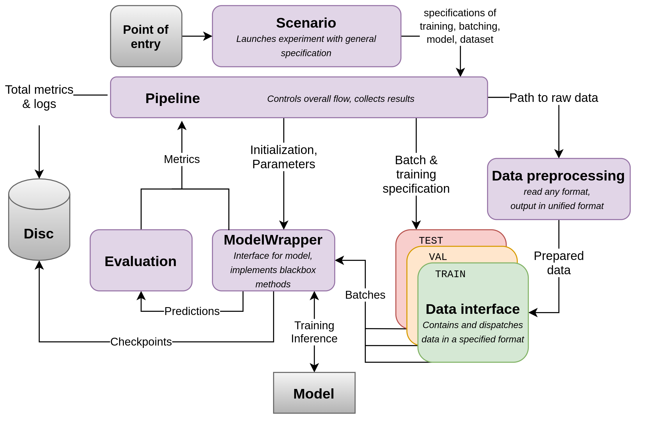
Figure 1. Diagram of the evaluation framework

Existing graph embedding models have been actively studied in recent years in attempts to apply deep learning methods for network representation learning. Hundreds of graph embeddings models have been developed in computer vision, text processing, recommendation systems, and interdisciplinary research in biology and genetics (I. and et al., 2021). All approaches are united by a common problem statement, which is to learn a model for the selected type of networks and important graph statistics. This will make it possible to apply standard machine learning frameworks and at the same time generalize attribute and structural information from the data.

Recently, modern machine learning methods have been proposed for processing networks and solving various prediction tasks on the local level. (N. and M., 2017; J. and et al., 2018b; P. et al., 2017; M. et al., 2018). Examples include node classification and link prediction, for nodes both seen and unseen during the process of model training. In practice, they represent important problems to be solved on large dynamic network data, for e.g., transaction data between companies and bank clients can be used to predict future transactions; user search history on the Web can be used to generate contextual advertising instances; disease transmission data can be used to predict epidemics dynamics.

Although most of the previous works on graph representation learning mainly focus on static graphs (with a fixed set of nodes and edges), there are many real-world applications in which graphs evolve over time, like social networks or sales data. One particularly common sub-type of graphs used to represent such structures is a temporal graph. It is a graph in which each edge has a time index, indicating a moment in time when the interaction, represented by an edge, occurred.

There are various problems when switching from static to dynamic networks (Rosenberg, 1981), among which computational complexity and variance of connectivity patterns over time. In addition, for practical applications, one needs to have models suitable for inference in inductive settings which enable proper prediction on the fly with rear overall model retraining for large network data (Kazemi S. M., 2020).

In this work, we describe a novel network embedding which combines the best elements of the efficient Temporal Graph Network embedding (TGN) (E. and et al., 2020) with fast computed historic node embeddings and highly precise Causal Anonymous Walks (CAW) (Y. and et al., 2021) with attention over temporal edge dynamics. To properly evaluate the proposed model, we present an experimental framework for temporal network embedding evaluation in downstream graph machine learning tasks, allowing integration of various temporal network embeddings and different temporal network data under a unified evaluation framework shown in Fig. 1.

Our main contributions with this work consist of the following:

1. Novel temporal network embedding model achieving state-of-the-art results in various temporal graph machine learning tasks;

2. Standardized temporal network embedding evaluation framework and comparison of state-of-the-art models under common training setting, providing new insights and clarification of real-world performance compared to reported in the original research articles.

In addition, we prove the effectiveness of the proposed pipeline and its sub-modules via extensive ablation study and provide the industrial application of the proposed approach, involving the transaction data of a major European bank. We showed that feature enrichment of temporal attention over temporal edge random walks improves both quantitative and qualitative results in the real-world application of a banking graph machine learning task.

2. Preliminaries & Problem statement

In order to proceed with the problem statement, we describe basic concepts used throughout the text following notations by (Kazemi S. M., 2020). We use $\mathcal{G}(\mathcal{V},\mathcal{E})$ to denote a static graph, where $\mathcal{V}$ is the set of its vertices, and $\mathcal{E}$ is the set of edges of the graph, and $\mathcal{A}$ is an adjacency matrix of that graph. Dynamic graph in general is a graph, which structure and node/edge attributes change over time. Generally, events may contain an updated state of the node, but in our experiments we consider all node features to be static, and represent them as $\mathcal{X}$ – $|V|\times k$ matrix, where $k$ is the node feature dimensionality.

In this work, we will use dynamic graph and temporal graph as interchangeable terms. We outline two possible kinds of dynamic graph representations below. There are two standard views on temporal network representation as a data structure:

• Discrete-time dynamic graph (DTDG) or snapshot-like graph is a sequence of snapshots from a dynamic graph, sampled at regularly-spaced times. Formally, we define DTDG as a set {$\mathcal{G}^{1}$, $\mathcal{G}^{2}$,…, $\mathcal{G}^{T}$, }, where $\mathcal{G}^{t}=\{\mathcal{V}^{t},\mathcal{E}^{t}\}$ is the graph at moment $t$, $\mathcal{V}^{t}$ and $\mathcal{E}^{t}$ are sets of nodes and edges in $\mathcal{G}^{t}$, respectively.

• Continuous-time dynamic graph (CTDG) or transaction-/stream-like graph is denoted by pair $(\mathcal{G},\mathcal{O})$, where G is a static graph representing an initial state of dynamic graph at time $t_{0}$, and $\mathcal{O}$ is event stream of events/transaction, denoted by tuple $(event\_coordinates,event\_data,timestamp)$, where $event\_coordinates$ are ordered pairs of nodes, between which the event has occurred, and $event\_data$ is any additional data on the event.

Event stream may be represented as concatenation of index matrix containing transactions vectors $e_{ij}(t)=(v_{i},v_{j},t)$ with source and target node IDs, timestamp, and temporal edges’ features.

We will refer to both CTDG and DTDG as dynamic graphs, although we will focus more on CTDGs as a natural representation of transactions in banking networks, which appear in non-uniform timestamps and represent a real-world streaming structured data, rather than discretized snapshot representation DTDG.

Finally, in our study, we consider such temporal graph machine learning problems as node classification and link prediction, both in transductive and inductive settings:

• Transductive edge prediction evaluates whether a transaction between two priorly known nodes occurred at a given time;

• Inductive edge prediction predicts a transaction between known and unknown nodes at a given time;

• Transductive node classification determines the dynamic label of a priorly known node;

• Inductive node classification determines the dynamic label of a priorly unknown node.

All the mentioned above problems on the chosen datasets can be formulated as binary classification (with effortless extension to a multi-class case), which is evaluated via AUC-ROC (area under curve for receiver operating characteristic) and AP (average precision) quality metrics measuring performance for the classification at various error threshold settings.

3. Related work

In this section, we overview state-of-the-art methods of constructing network embeddings for static and dynamic networks using taxonomies suggested in (I. and et al., 2021) and (DT et al., 2021). We focus on dynamic network embedding as an evolutionary process of graph formation.

3.1. Static graph embedding methods

When constructing network embeddings via solving the optimization problem, researchers usually focus on three main concepts: matrix factorization, node sequence methods and methods based on deep learning. We consider the snapshot method, in which the current snapshot of a temporal network is taken and missing links are predicted based on the available graph information.

Factorization techniques can be applied to different graph representations and optimized for different objectives, such as direct decomposition of the graph adjacency matrix (Kruskal, 1978; S. and et al., 1990; M. and C., 2001) or approximating proximity matrix (T. and K., 2000; B. et al., 2000). Despite factorizations being widely used in recommendation systems, these models have high computational complexity and are difficult to extend for inductive learning.

Inspired by word2vec (T. and et al., 2013), sequence-based methods aim to preserve local node neighborhoods based on random walks. The two most prominent examples of models in this class are DeepWalk (B. et al., 2014) and Node2vec (A. and J., 2016). Anonymous graphs walks have been proposed in (Ivanov and Burnaev, 2018). However, their adaptations to temporal random walks have limited applications, since they require retraining after adding new edges.

Recently, advances in geometric deep learning led to the creation of graph neural networks combining the best out of both fully connected and convolutional neural network architectures. Most of them use the method of neighborhood information aggregation from graph convolution network (GCN) (N. and M., 2017) and extend it with classical deep learning architectures such as recurrent neural network (RNN) (J. and et al., 2018b), attention mechanism (P. et al., 2017), generative adversarial network (GAN) (M. et al., 2018), and graph transformers (Yun et al., 2019).

Recent studies show that a combination of deep learning models with semi-supervised techniques gives state-of-the-art results in terms of scalability, speed and quality in downstream tasks (I. and et al., 2021). However, static models are limited by the necessity to retrain the model with each significant change of graph structure.

3.2. Dynamic graph embedding methods

Methods for dynamic graphs are often extensions of those for static ones, with an additional focus on the temporal dimension and update schemes (A. and et al., 2020a). All these techniques can be categorized according to which model of graph evolution representation is chosen: Continuous-Time Dynamic Graphs (CTDG) or Discrete-Time Dynamic Graphs (DTDG).

3.2.1. DTDG-focused methods

Most of the early work on dynamic graph learning focuses exclusively on discrete-time dynamic graphs. Such models encode snapshots individually to create an array of embeddings or aggregate the snapshots in order to use a static method on them (U. and J., 2008). All DTDG models can be divided into several categories, according to the approach they use for dealing with the temporal aspect of a dynamic graph.

Single-snapshot models. Static models are used on the graph snapshots to make predictions for the next one ((L. and et al., 2018; S. and et al., 2018; P. and et al., 2018)). Another way of implementing this methodology, called TI-GCN (Time Interval Graph Convolutional Networks) via residual architectures was proposed in (R., 2018; Y. et al., 2020a). Besides single snapshots, these works use information from networks formation (R., 2018) represented by edge differences of several snapshots.

Multi-snapshot models. In (M. and et al., 2020; S. et al., 2019a), authors learn structural information of each snapshot by separate models. Authors of (M. and et al., 2020) compute individual sets of random walks for each snapshot in Node2Vec fashion and learn final node embeddings jointly, while in (S. et al., 2019a) autoencoders for each snapshot were trained in a consistent way to preserve similarity between consequent graph updates.

RNN-based models. In contrast to previous methods, models in this category aim to capture sequential temporal dependencies mostly by feeding the output node embeddings or graph structure of each snapshot into RNN. Thus, GCN is combined with long short-term memory (LSTM) in (F. et al., 2020; J. and et al., 2018a; Y. and et al., 2016) or gated recurrent units (GRU) in (L. and et al., 2019; Y. and et al., 2018). Following these ideas, authors of (S. and et al., 2019; C. and et al., 2019) add residual connections to propagate topological information between neighboring snapshots. Recently, some works (K. and et al., 2019; A. and et al., 2019) have proposed to use GANs in combination with RNNs. On the other hand, EvolveGCN (A. and et al., 2020a) argues that directly modeling dynamics of the node representation will hamper the model performance on graphs with dynamic node sets. Instead of treating node features as the input to RNN, it feeds the weights of the GCN into the RNN.

Temporal graph attention. Inspired by advances in natural language processing (NLP), models in this class leverage attention-mechanism to capture temporal information. In (J. and et al., 2020, 2019; H. and et al., 2020), authors follow the RNN module by an attention mechanism to take into account the contribution of its hidden states or leverage self-attention mechanism without RNN stage (A. and et al., 2020b).

Convolutional models. Although previous models can capture sequential dependencies, in practice, most of them use a limited number of historical snapshots. So, convolutions are used to propagate information between snapshots in (B. et al., 2018; Fathy and et al., 2020; Z. and et al., 2021b).

Despite promising results, most of the models struggle from two disadvantages. First, methods lose the order of edge formation and reflect only partial information on network formation (Y. et al., 2020a). Second, computing static representations on each snapshot is inefficient in terms of memory usage on large graphs (Z. and et al., 2021a) and can not be used in practical applications.

3.2.2. CTDG-focused methods

Continuous-time dynamic graphs require different approaches as it becomes computationally difficult to work with the entirety of such graphs after each interaction (R. and et al., 2019a). Below we provide a more general classification of CTDG-focused methods, comparing with DTDG-focused ones based on approaches used for learning evolution patterns.

Temporal random-walks models. The approach implies including the time dependency directly in a sequence of nodes generated by random walks. Such methods create a corpus of walks over time (so-called ”temporal random walks”) with respect to the order of nodes/edges appearance in the graph. Based on this idea, authors of (S. and et al., 2020) leverage a custom attention mechanism to learn the importance between a node and its temporal random-walk-based neighbors. Using this work, (H. and et al., 2018) proposes several methods to select the subsequent nodes connected to a starting one. A promising method for link prediction task was proposed by the authors of (Y. and et al., 2021) who have developed Causal Anonymous Walks (CAWs), constructed from temporal random walks. CAWs adopt a novel anonymization strategy that replaces node identities with the hitting counts of the nodes based on a set of sampled walks to keep the method inductive. The model outperforms previous methods in both inductive and transductive settings.

Local neighborhood models. When interactions happen (node or edge adding and removal), models in this class update embeddings of the relevant nodes by aggregating information from their new neighborhoods. In (Z. and et al., 2021a; L. and et al., 2020), authors utilize a GCN-based aggregation scheme and propagate changes to higher-order neighbors of interacting nodes. To cope with information asymmetry, the authors of (H. and et al., 2021) propose to determine the priority of the nodes that receive the latest interaction information. Models from (S. et al., 2019b; D. and et al., 2020) embed dynamic network for recommendation systems in similar ways. Several recent works (R. and et al., 2019b; B. et al., 2019; Y. and et al., 2019) consider interactions between nodes as stochastic processes with probabilities depending on the network statistics.

Memory-based models. The core idea of this class of temporal network embeddings lies in extending existing models by using special memory modules storing a history of interactions for each node. Methods vary from updating LSTM (Y. et al., 2020b) to using augmented matrices of interactions (Z. and et al., 2020). APAN (Asynchronous Propagation Attention Network) (X. and et al., 2021) aims to store detailed information about k-hop neighborhood interactions of each node in so-called ”mailboxes”. The recently developed temporal graph network (E. and et al., 2020) proposes a flexible framework, which consists of several independent modules and generalizes other recent CTDGs-focused models such as (D. and et al., 2020; S. et al., 2019b; R. and et al., 2019b). Combining the advantages of JODIE (S. et al., 2019b) and temporal graph attention (TGAT) (D. and et al., 2020), TGN introduces the node-wise memory into the temporal aggregate phase of TGAT, showing state-of-the-art for industrial tasks results.

Because of the potential of CTDG-based models (J. and B., 2021) and necessity to apply the model to transaction data, we focus on developing a model in this class, while keeping in mind efficient DTDG models (Y. et al., 2020a). In what follows, we describe the idea of improving existing state-of-the-art CTDG models by properly fusing memory-based, neighborhood and interaction information under unified framework, thus combining multiple best practices of CTDG methods.

4. Proposed Approach

As stated above in our literature survey, the best-known model for temporal graph prediction tasks, namely, TGN (E. and et al., 2020), relies primarily on propagating information (”message”) through edges and generates node embeddings from occurring edges in a straightforward manner. At the same time, it was noticed that the CAW (Y. and et al., 2021) shows excellent performance in link prediction tasks by learning edge representations. Unfortunately, the latter model cannot be directly applied to the extraction of node embeddings, and, consecutively, downstream graph machine learning tasks, such as node classification.

Hence, in this paper, we propose a novel network embedding taking the best out of the TGN framework and the CAW edge encodings (Fig. 2) to improve the quality of edge and node classification. Our contribution is to leverage the highly informative edge embedding generated in CAW. This will allow us to refine various functions of the TGN framework, including generating messages and embeddings, as well as aggregating memory.

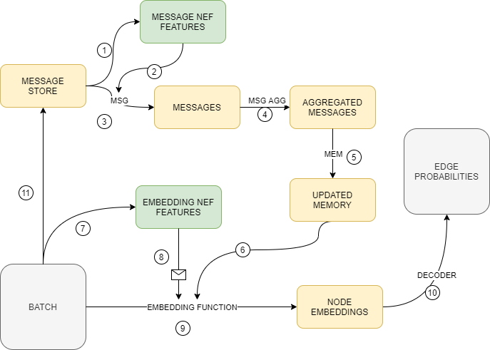
Figure 2. Proposed model; numbers denote order of steps

4.1. Model details

Below, we describe our model by listing and describing all modules in a consecutive fashion. In the following descriptions and equations, LSTM refers to the Long Short-Term Memory type RNN, GRU is the Gated Recurrent Unit, ”attn” and ”self-attn” is attention and self-attention, respectively. A walk on a graph, performed backwards in time on a temporal graph (time-inverse walk) with length $M$ is denoted by

(1) $$W=((w_{0},t_{0}),(w_{1},t_{1}),..,(w_{M},t_{M})),t_{0}>t_{1}>\textperiodcentered\textperiodcentered>t_{M},\\ ({w_{m-1},w_{i}},t_{m})\in\mathcal{E},m\in\{1,2,...,M\}$$

where $w_{m}\in\mathcal{V}$ is the node entered at step $m$, $t_{m}$ is the time of step $m$, $(w_{m},t_{m})$ is the $m$-th node-time pair. In future, we will refer to the elements of the $m$-th step as $W_{m}^{(1)}=w_{m}$ and $W_{m}^{(2)}=t_{m}$.

The $t$-timed $k$-hop neighborhood of $i$-th node is a set of nodes which can be reached from $i$ in $k$ steps if one walks on the edges existing prior to time $t$, without regard for their direction:

(2) $$\eta_{i}^{k}=\{w_{j}:\exists W=((w_{0},t_{0}),...,(w_{j},t_{j})),w_{0}=i,\forall l:t_{l}<t,\\ ({w_{p-1},w_{p}},t_{p})\in\mathcal{E}\vee({w_{p},w_{p-1}},t_{p-1})\in E,|W|\leq k+1\}$$

4.1.1. Neighborhood Edge Feature (NEF) Generator)

This trainable module and its integration in the following modules are intended to improve the predictive capabilities of the original TGN framework, which is our core contribution. It generates highly informative feature representations of pairs of nodes for any given moment in time. For a pair of nodes $i$ and $j$, the output of this module as $NEF_{ij}(t)$ is computed as follows.

At first, we sample an equal number $K>1$ of the time-inverse walks for both nodes in order to capture information about the edge neighborhoods. All sampled walks have identical lengths (1-2 steps typically). A constant decay hyperparameter, which regulates how strongly the sampling process prioritizes more recent connections, is used during sampling of all walks.

The walk sets $S_{i}$ and $S_{j}$ are generated for edge $ij$ between nodes $i$ and $j$. $S_{i}$ consists of sampled time-inverse walks $W_{k},k\in\{1,...,K\}$. Each edge for each walk is sampled with the probabilities proportional to $exp(\alpha\triangle t)$, where $\alpha$ is the decay parameter, and $\triangle t$ is the time difference between edges.

The next step makes the sampled walks anonymous in order to limit extracted information to the edge neighborhood alone. Each node from $S_{i}$ is replaced by a pair of vectors that encode a positional frequency of the node in each corresponding position of walks in $S_{i}$ and $S_{j}$. The encoding vector of positional frequencies relative to the walks of $i$ for node $w$ is defined as:

(3) $$g(w,S_{i})=\{|\{W|W\in S_{i},w=W_{m}^{(1)},m\in\{1,...,M\}\}|\}.$$

This equation simply specifies that the node index $w$ is encoded as a vector, so that each its $m$-th component is equal to the number of times where $w$ is the $m$-th node of some walk in $S_{i}$.

The anonymization of walks (Y. and et al., 2021) is achieved by using the defined function to transform node indices in walks. Each position in any walk of $S_{i}$ containing $w$ is replaced by

(4) $$I^{ij}(w)=\{g(w,S_{i}),g(w,S_{j})\}.$$

Similarly, any value in walks of $S_{j}$ filled by $w$ is replaced with $I^{ji}(w)$. In the remaining part of this section we write $I=I^{ij}$, assuming the known orientation of the edge.

The remaining steps simply attempt to transform the “anonymous walk” representation of the node pair to a more compressed and usable state. Each obtained representation of each position of each walk, i.e. pairs of $\{g(w,S_{j}),g(w,S_{i})\}$, are fed through separate instances of the same two-layered multi-layered perceptron (MLP) and sum-pooled:

(5) $$f_{1}(I(w))=\operatorname{MLP}(g(w,S_{i}))+\operatorname{MLP}(g(w,S_{j}))$$

Then, this representation is concatenated with the time-difference encoding and node or edge features of the corresponding step:

(6) $$h(I(w))=\operatorname{concat}(f_{1}(I(w)),f_{2}(\triangle t),X)$$

where $f_{2}(\triangle t)$ is time Fourier features, and $X$ is a concatenation of all relevant node and edge attributes of the corresponding walk step. Finally, each walk with encoded positions is passed to an RNN (usually, Bi-LSTM):

(7) $$\operatorname{enc}(W)=\operatorname{Bi-LSTM}(\{h(I(w_{m})),m\in\{1,...,M\}\}),$$

where $w_{m}$ being $m$-th position of walk $W$.

The encoded walks are aggregated across all walks for the node pair $ij$:

(8) $$NEF_{ij}(t)=\frac{1}{|S_{i}\cup S_{j}|}\sum_{W\in(S_{i}\cup S_{j})}{\operatorname{agg}(\operatorname{enc}(W)}),$$

where $|S_{i}\cup S_{j}|$ is amount of walks in a set $S_{i}\cup S_{j}$, and $\operatorname{agg}$ is either self-attention module or identity for mean pooling aggregation.

4.1.2. Message store

In order to apply the gradient descent, a memory of a node should be updated after it is passed as a training instance. Let’s say an event associated with the $i$-th node has occurred, e.g. an edge involving $i$ has been passed for training in the current batch. Then, all information about the batch transactions involving node $i$ will be recorded in the message store after the batch inference, replacing the existing records for $i$. This information is used and updated during the processing of the next batch involving $i$.

4.1.3. Message Generator

When the model processes a batch containing a node, all transaction information about edges associated with this node is pulled. For each transaction between $i$ and some other node $j$ at a time $t$, a message for a node $i$ is computed as a concatenation of the current memory vectors of the nodes, edge features, time-related features, and neighborhood edge features of the corresponding edge:

(9) $$m_{i}(t)=concat(s_{i}(t^{-}),s_{j}(t^{-}),t-t^{-},e_{ij}(t),NEF_{ij}(t)),$$

where $ij$ is the index of a transaction between nodes $i$ and $j$, $s_{i}(t^{-})$ is a memory state of node $i$ at time $t^{-}_{i}$ of last memory update for node $i$, and $NEF_{ij}(t)$ is a neighborhood edge feature vector for edge $ij$. The usage of NEF features here is our novel idea aimed to include more information about the type of the update message. The generated messages will update memory states of the batch nodes. Note that, aside from the basic and non-trainable concatenation, other choices for the message function, like MLPs are possible.

4.1.4. Message Aggregator

To perform a memory update on a node at time $t$, its message representation is obtained by aggregating all currently stored messages timestamps $t_{1}<t_{2}<...<t$ which are related to this node:

(10) $$\overline{m}_{i}(t)=\operatorname{aggr}(m_{i}(t_{1}),m_{i}(t_{2}),...,m_{i}(t)).$$

Here aggregation function $aggr$ can be computed as a mean of generated messages. It is still possible to use the most recent message $m_{i}(t)$ as a value of $\overline{m}_{i}(t)$.

4.1.5. Memory Updater

The message generator and aggregator let the model to encode useful transaction information as memory vectors. In particular, the memory state vector for node $i$ is updated at time $t$ by applying an RNN-type model to the concatenation of the received message and previous memory state:

(11) $$s_{i}(t)=\operatorname{RNN}(\overline{m}_{i}(t),s_{i}(t^{-}))$$

where $\operatorname{RNN}$ is either GRU or LSTM, and initial state $s(0)$ is initialized with a random vector.

4.1.6. Embedding Generator

This module generates the node embedding based on memory states of the node and its k-hop neighborhood, features of the neighborhood, and NEF representations of ”virtual” edges between the node and its direct neighbors. Resulting node embeddings can be viewed as autonomous node representations for classification. We propose, similarly to message generator, to add NEF features to node $i$ in order to let the model better discriminate neighbors on their relevance or type:

(12) $$z_{i}(t)=\sum_{j\in\eta_{i}^{1}}h_{0}(s_{i}(t),s_{j}(t),e_{ij},v_{i}(t),v_{j}(t),NEF_{ij}(t))+\\ \sum_{j\in\eta_{i}^{k},k>1}h_{1}(s_{i}(t),s_{j}(t),e_{ij},v_{i}(t),v_{j}(t)),$$

where $v_{i}(t)$ is a feature vector of node $i$ at time $t$, and $h_{0}$ and $h_{1}$ are the units of the neural network. It is typical to use MLPs as $h_{0}$ and $h_{1}$, but the following concatenation by self-attention is more preferable to capture complex dependencies involving NEFs.

4.1.7. Embedding Decoder

This is the final module, which transforms node embeddings into prediction results for downstream tasks. In this paper, we always use MLP with 3 layers with only node embeddings as inputs, and sigmoid or softmax output layers. For example, the multi-class classification problem for node $i$ at time $t$ is solved using the following equation:

(13) $$out_{i}(t)=\operatorname{Softmax}(\operatorname{MLP}(z_{i}(t))).$$

Similarly, the edge prediction task is solved as follows:

(14) $$out_{ij}(t)=\operatorname{Sigmoid}(\operatorname{MLP}(\operatorname{concat}(z_{i}(t)z_{j}(t)))).$$

4.2. Core idea and novelty of proposed model

Let us provide a high-level description of the model (Fig. 2). It learns to generate a temporal embedding for each node and decode embeddings into inputs for each classification task. The model assigns a memory vector to each node and generates each node embedding by aggregating memory vectors and other relevant features in a neighborhood of the node. Node memory vectors describe relevant information about interactions involving the node. They are updated using specified node messages, which, in turn, encode information about the last transaction involving the node. This design allows employing gradient descent for training memory and message generating modules. A decoder MLP transforms a pair of node embeddings into the probability of a temporal edge existing between the nodes. Similarly, it can be trained to transform a single node embedding into probabilities of the node belonging to each of the existing classes for a node classification problem.

There are two main modifications of the proposed model compared to the baseline TGN framework (E. and et al., 2020). First, we change the message generating function, which provides the model with an additional way to differentiate the messages based on their relevance. The NEF features of an edge contain information about the walk correlation of the two nodes. As it can be used for very accurate link prediction (Y. and et al., 2021), it may be also used to classify some messages as being irrelevant, and diminish their effect on the memory update.

Second, while the original version of the embedding module (E. and et al., 2020) allows treating different k-hop neighbors of the node differently if using attention for aggregation, it might be beneficial to provide the NEF features of connections between the node and its closest neighbors. As a result, we again take into account the walk correlation between the node and its neighbor, so that the differences in neighborhood type can be more evident.

Table 1. Dscriptive statistics for the dataset. Left to right: whether the graph is bipartite, number of unique nodes (representing users and items) and edges, labels, average degree, number of edge updates per node as source/target, and setting for splitting the temporal network into batches for snapshot DTDG models

	Bipartite	Unique nodes	Unique edges	Positive labels / Fraction	Average degree	Average edges per n ode	Batch setting
Reddit	Yes	10000 / 984	672447	366 / 0.0005	61.372	67.244 / 683.381	1 day per batch (30 days total)
Wikipedia	Yes	8227 / 1000	157474	217 / 0.0013	17.192	19.141 / 157.474	1 day per batch (30 days total)
Enron	No	185	125236	-	29.059	675.778	1% of total edge count
UCI	No	1900	59836	-	106.405	13.043	1% of total edge count
Ethereum	No	231288	300000	-	2.339083	2.59416	1% of total edge count

5. Evaluation framework

In this section, we discuss our research methodology. This involves the evaluation framework, evaluation pipeline training settings, hyper-parameter choice and description of temporal networks used for the evaluation.

5.1. Pipeline

The main contribution of the proposed framework (Fig. 1) is an easy-to-use unified data processing toolkit for accurate evaluation of temporal network embeddings in downstream tasks under common training settings, which allows to remove contradictions in experimental results reported in research articles in the field. The source code of this tool is publicly available. It is focused on transforming any graph into a universal format that is afterwards fed into the pipeline in either DTDG or CTDG format with following features:

• selection of precise batching options;

• preparing data for both inductive and transductive settings (with support for bipartite data);

• interfacing with any kind of graph embedding models using an interface for model-framework communication, treating network embedding models as a black-box, which is then passed on to such basic methods as train_model, predict_edge_probabilities, etc.

5.2. Training settings

5.2.1. Negative sampling

It is common to design include negative edge sampling into evaluation of temporal graph prediction tasks. It is employed for balancing edges and non-connected pairs of nodes. We follow a standard setting, where the number of negative samples is equal to the number of edges.

5.2.2. Batch specification

The model is trained by passing edges (which includes negative samples) in batches sorted in chronological order.

5.2.3. Training with temporal data masking

We use 80%-10%-10% train-val-test split with randomized training sets, supported via several data masking schemes. Node masking hides nodes (as well as all connected edges) from training data. The masked nodes for transductive tasks are also removed from the validation and test data, while for inductive tasks masked nodes remain in validation and test data. Edge masking removes a fixed percentage of random edges from the whole dataset. We use two options for both masking techniques: the percentage of masked information is 10% and 70%, representing dense and sparse training settings, respectively. In particular, we report the results for three combinations, in which at least one mask is large, namely 10%-75% node-edge masking, 75%-10% and 75%-75%.

5.2.4. Runs and validation

Each model/setting/dataset combination was run 10 times with random seeds and node/edge masking.

5.3. Comparison with the state-of-the-art models

In order to evaluate our model (Fig. 2), we compare it to the baseline TGN framework architectures (configured as described in (E. and et al., 2020)), DyRep (supporting long-term and short-term time scales of graph evolution and scaling to large graphs) (R. and et al., 2019b) and Jodie (working with bipartite graphs using node embeddings for predictive tasks with future time lag) (S. et al., 2019b). Though these models can construct high-quality historic embeddings using information propagated from nodes, they do not take into account edge information and interaction patterns. Hence, we could demonstrate the advantages of our approach in identical training settings in comparison to other state-of-the-art temporal network embeddings. It is important to emphasize that the CAW model cannot be used here because it was created only for graph reconstruction tasks and cannot produce node/edge embeddings for the downstream tasks.

5.4. Datasets

In our study, we focus on well-known benchmark datasets for temporal networks. Their descriptive statistics are presented in Table 1, taking into account specifics of computing statistics for bipartite graphs of user-item interactions (M. et al., 2008).

Labeled datasets

Both Reddit (L. et al., 2017) and Wikipedia (Foundation, 2010) datasets are bipartite graphs representing interactions between users (source) and web resources (target), like posting to a subreddit or editing a wiki page. Text content is encoded as edge features to provide context. Both datasets have a binary target, indicating whether a user was banned or not.

Non-labeled datasets

The UCI (P. and G., 2008) dataset contains a communication history for the students’ forum. The Enron (J. and et al., 2008) dataset is constructed over internal e-mail communication of Enron company employees. The Ethereum dataset contains a directed graph of Ethereum blockchain transactions, which were collected from larger public BigQuery dataset; we collected a dataset containing all transactions, which occurred during a 9-hour span. All of the non-labeled datasets are non-bipartite, with no additional features for edges or nodes.

6. Ablation study

In this Section an ablation study of the proposed architecture (Fig. 2) is provided to explore the impact of each submodule. Below we specify several additional modules added to interaction features processing pipeline for temporal network embedding via NEF generator,which outlined in Subsection 4.1.1:

• NEF-Message concatenating NEF features and messages;

• NEF-Embed generates embeddings with NEF features;

• NEF-LSTM including Bi-LSTM into NEF generator, instead of mean pooling across walk elements.

Additionally, we consider alternating three important NEF-related hyper-parameters:

• number of generated random walk NEF-samples;

• random walk depth;

• positional dimension of random-walk-related embeddings.

Table 2 contains AUC-ROC standard deviation and mean averaged 10 times. The task measured was inductive edge prediction with default hyperparameters. Rather large and representative Reddit dataset is used in ablation study. Below we provide performance metrics for seven different combinations of modules mentioned above, except ”(RNN)”, which is considered a standalone TGN with NEF features processing regularization. Here the resulting model significantly improves the performance of standalone modifications and TGN baseline.

Table 2. Ablation study on Reddit dataset for inductive edge prediction

Enabled modules	AUC-ROC
(Msg)+(Emb)+(RNN)	$0.894\pm 0.034$
(Emb)	$0.893\pm 0.035$
(Msg)	$0.888\pm 0.042$
(Emb)+(Msg)	$0.878\pm 0.051$
(Msg)+(RNN)	$0.876\pm 0.047$
(Emb)+(RNN)	$0.870\pm 0.055$
TGN baseline	$0.865\pm 0.065$

7. Experimental results

In this section, we compute mean AUC-ROC and AP for our model and compare it to three other state-of-the-art models (DyRep, Jodie, TGN). Tables 3-Table 6 show results for edge prediction task in transductive and inductive settings respectively. Best results are given in bold, while second best are underlined. ”Node mask” and ”Edge mask” columns specify the portion of nodes or edges used for model testing.

Table 3. Transductive edge prediction, AUC-ROC; best in bold, second-best underlined

	Node mask	Edge mask	DyRep	Jodie	TGN	Our
Enron	10%	75%	0.774	0.534	0.638	0.759
	75%	10%	0.647	0.528	0.682	0.795
	75%	75%	0.595	0.537	0.673	0.745
Reddit	10%	75%	0.964	0.704	0.974	0.977
	75%	10%	0.973	0.825	0.977	0.977
	75%	75%	0.959	0.72	0.976	0.977
UCI	10%	75%	0.77	0.496	0.804	0.808
	75%	10%	0.731	0.573	0.709	0.812
	75%	75%	0.781	0.489	0.776	0.808
Wikipedia	10%	75%	0.966	0.728	0.968	0.969
	75%	10%	0.964	0.737	0.971	0.975
	75%	75%	0.962	0.719	0.967	0.97
Ethereum	10%	75%	0.728	0.914	0.932	0.933
	75%	10%	0.868	0.929	0.936	0.937
	75%	75%	0.73	0.919	0.934	0.934

Table 4. Transductive edge prediction, AP; best in bold, second-best underlined

	Node mask	Edge mask	DyRep	Jodie	TGN	Our
Enron	Lean	Strict	0.772	0.517	0.651	0.762
	Strict	Lean	0.668	0.527	0.685	0.787
	Strict	Strict	0.6	0.524	0.699	0.753
Reddit	Lean	Strict	0.965	0.688	0.973	0.977
	Strict	Lean	0.974	0.832	0.977	0.977
	Strict	Strict	0.96	0.699	0.977	0.977
UCI	Lean	Strict	0.804	0.503	0.827	0.826
	Strict	Lean	0.756	0.546	0.75	0.824
	Strict	Strict	0.812	0.492	0.809	0.827
Wikipedia	Lean	Strict	0.969	0.708	0.971	0.972
	Strict	Lean	0.966	0.711	0.974	0.976
	Strict	Strict	0.965	0.695	0.969	0.973

Table 5. Inductive edge prediction, AUC-ROC; best in bold, second-best underlined

	Node mask	Edge mask	DyRep	Jodie	TGN	Our
Enron	10%	75%	0.613	0.453	0.591	0.677
	75%	10%	0.672	0.508	0.705	0.792
	75%	75%	0.666	0.573	0.702	0.766
Reddit	10%	75%	0.832	0.588	0.823	0.836
	75%	10%	0.91	0.294	0.917	0.924
	75%	75%	0.88	0.298	0.907	0.917
UCI	10%	75%	0.602	0.576	0.599	0.642
	75%	10%	0.723	0.431	0.725	0.733
	75%	75%	0.718	0.423	0.735	0.74
Wikipedia	10%	75%	0.95	0.584	0.945	0.953
	75%	10%	0.902	0.462	0.899	0.918
	75%	75%	0.888	0.47	0.894	0.911
Ethereum	10%	75%	0.519	0.655	0.677	0.679
	75%	10%	0.483	0.629	0.656	0.667
	75%	75%	0.494	0.616	0.654	0.654

Table 6. Inductive edge prediction results, AP; best in bold, second-best underlined

	Node mask	Edge mask	DyRep	Jodie	TGN	Our
Enron	10%	75%	0.649	0.527	0.627	0.689
	75%	10%	0.668	0.524	0.712	0.785
	75%	75%	0.678	0.566	0.71	0.765
Reddit	10%	75%	0.858	0.582	0.851	0.86
	75%	10%	0.924	0.393	0.931	0.936
	75%	75%	0.899	0.391	0.917	0.928
UCI	10%	75%	0.664	0.576	0.663	0.69
	75%	10%	0.762	0.46	0.763	0.771
	75%	75%	0.756	0.461	0.773	0.773
Wikipedia	10%	75%	0.952	0.551	0.949	0.954
	75%	10%	0.914	0.473	0.905	0.927
	75%	75%	0.9	0.479	0.906	0.916

As evident from above figures, the proposed approach (Fig. 2) consistently outperforms almost all other models. For example, our model achieves the best results in transductive edge prediction (Table 3) except one case, where DyRep achieved better results. Moreover, our method achieves the best results on all datasets for inductive edge prediction (Table 5). It seems that capturing network-wide common patterns with CAW-based features generally offers an improvement over existing models, although in some cases information added by these features may be duplicated by other encoding modules.

Table 7. Transductive node classification, AUC-ROC; best in bold, second-best underlined

	Node mask	Edge mask	DyRep	Jodie	TGN	Our
Reddit	10%	75%	0.531	0.421	0.635	0.659
	75%	10%	0.601	0.435	0.584	0.627
	75%	75%	0.597	0.439	0.602	0.658
Wikipedia	10%	75%	0.771	0.842	0.735	0.81
	75%	10%	0.769	0.836	0.738	0.8
	75%	75%	0.755	0.855	0.8	0.823

Table 8. Inductive node classification, AUC-ROC; best in bold, second-best underlined

	Node mask	Edge mask	DyRep	Jodie	TGN	Our
Reddit	10%	75%	0.51	0.456	0.576	0.625
	75%	10%	0.544	0.539	0.495	0.563
	75%	75%	0.521	0.567	0.592	0.584
Wikipedia	10%	75%	0.749	0.883	0.638	0.812
	75%	10%	0.619	0.73	0.649	0.766
	75%	75%	0.665	0.743	0.597	0.745

Table 7 and Table 8 present the results for node classification tasks in transductive and inductive settings respectively. Though our model generally outperforms existing methods, there is one exception. Indeed, Jodie (S. et al., 2019b) shows the best node classification quality on Wikipedia dataset. As a matter of fact, the Jodie model incorporates both static and dynamic node embeddings, which might contributed to better encoding of interests and behavior patterns of the Wikipedia editors

8. Banking results

As an industrial application of the proposed framework, we chose a pre-existing problem posited by a major European banks with a corresponding dataset which consists of transactions between different companies. Each transaction has a timestamp so we can treat it as a temporal edge. This allows us to consider only ”edge events”. We use the following edge features: transaction amount, timestamp and type of transaction, (e.g. credit or state duty). We one-hot encode the type of transaction, which gives us 50 edge features in total: 49 from one-hot encoding and 1 from transaction amount. These features were normalized.

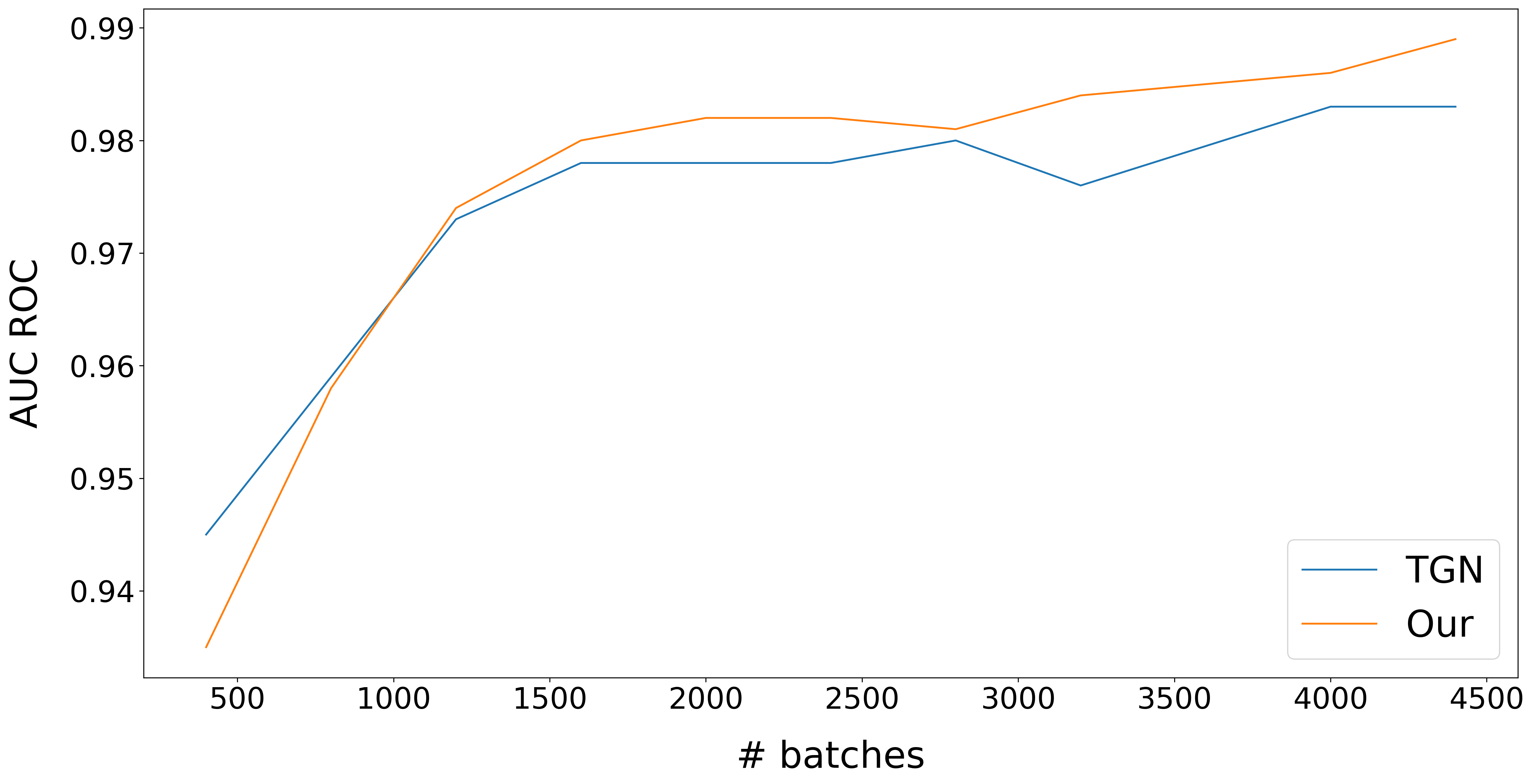
Figure 3. Inductive edge prediction on transactions of regional subdivision of major European bank

At first, we compared our model with the original TGN (E. and et al., 2020) on a link prediction task. We obtain the training and validation datasets consisting of transactions from a regional subdivision of a major European bank for a time period about one week. This dataset contain about 2 millions of transactions. We select about 40000 newest transactions to test dataset and all the rest is given to the train i. e. test dataset transactions are always newer then train transactions. We use the following procedure to check performance of our model on test dataset. First, we split training data into small chunks (400 batches) and gradually increase the number of chunks used to train the model. Each batch contains 512 transactions. The results are presented in Fig. 3.

We can see very high performance of dynamic graph approach models. It can be noticed that performance of our model grows a little bit slower than for TGN (E. and et al., 2020), but after about 600000 transactions our model takes the lead. This slight time lag in training is due to our model taking additional time to learn extra information about interactions between nodes via learning CAW (Y. and et al., 2021) part of our model. This extra information allows to gain better results in the end of training.

Table 9. Node classification results based on node embeddings obtained from TGN and our proposed model with feature dimension $d$ being multiple of $8\times 2$ shape

Node Embeddings	AUC-ROC
TGN	$0.626\pm 0.072$
Our, $d=10$	$0.653\pm 0.049$
Our, $d=20$	$0.598\pm 0.067$
Our, $d=100$	$0.578\pm 0.094$

The architecture of our model and TGN (E. and et al., 2020) model allows us to produce node embeddings which can the be used as input for a wide range of possible downstream tasks. For our experiment we have taken prediction of company default as the downstream task. The dataset contains about 5000 companies, some of which will go bankrupt in a specific period of time in the future (180 days) and others will not. To train a classification model we used LightGBM (Ke et al., 2017). The obtained results were averaged over with 5-fold cross-validation and presented in Table 9.

Here our best model has $2.7\%$ higher AUC ROC when compared to the TGN (E. and et al., 2020). That means that extra information about interactions between nodes captured by CAW (Y. and et al., 2021) part of our model is useful for classification problems. We see also that best performance is observed with small CAW messages shape. This is related to the structure of our dataset. It’s number of edges is comparable with number of nodes, thus the graph is sparse. Bigger CAW messages shapes can be useful for more dense graphs.

9. Conclusion

In this work, we proposed a novel model for temporal graph embedding (Fig. 2) that shows improvement over existing methods (E. and et al., 2020; R. and et al., 2019b; S. et al., 2019b) on various prediction tasks while preserving the ability to generate node embeddings. Moreover, we implemented a novel experimental framework (Fig. 1) that can process most kinds of graph data and an arbitrary dynamic graph inference model. Experimental study demonstrates the applicability of our method to solving various node/edge prediction tasks on temporal networks, and significantly improving the existing results.

In future, it is possible to improve the performance of our framework for its application to the real-life temporal graph of bank’s transactions with tens of billions of nodes. It is necessary to study efficient node/edge sampling strategies, choosing those that overcome the limitations of current models when scaling to large graphs while preserving highly-informative edge features propagation.

References

- (1)
- A. and J. (2016) Grover A. and Leskovec J. 2016. node2vec: Scalable Feature Learning for Networks. arXiv:1607.00653 [cs.SI]
- A. and et al. (2019) Maheshwari A. and et al. 2019. DynGAN: Generative Adversarial Networks for Dynamic Network Embedding. In Graph Representation Learning Workshop at NeurIPS.
- A. and et al. (2020a) Pareja A. and et al. 2020a. EvolveGCN: Evolving Graph Convolutional Networks for Dynamic Graphs. Proceedings of AAAI-20 Conference on AI 34 (2020), 5363–5370.
- A. and et al. (2020b) Sankar A. and et al. 2020b. DySAT: Deep Neural Representation Learning on Dynamic Graphs via Self-Attention Networks. In Proceedings of ACM IC on WSDM (WSDM ’20). 519–527.
- B. et al. (2019) Knyazev B., Augusta C., and Taylor G. W. 2019. Learning Temporal Attention in Dynamic Graphs with Bilinear Interactions. arXiv:1909.10367 [stat.ML]
- B. et al. (2014) Perozzi B., Al-Rfou R., and Skiena S. 2014. Deepwalk: Online learning of social representations. In Proceedings of ACM SIGKDD IC on KDD’20. 701–710.
- B. et al. (2000) Tenenbaum J. B., De Silva V., and Langford J. C. 2000. A global geometric framework for nonlinear dimensionality reduction. science 290, 5500 (2000), 2319–2323.
- B. et al. (2018) Yu B., Yin H., and Zhu Z. 2018. Spatio-Temporal Graph Convolutional Networks: A Deep Learning Framework for Traffic Forecasting. In Proceedings of IJCAI-18. International Joint Conferences on Artificial Intelligence Organization, 3634–3640.
- C. and et al. (2019) Chen C. and et al. 2019. Gated Residual Recurrent Graph Neural Networks for Traffic Prediction. Proceedings of AAAI-19 Conference on AI 33, 01 (2019), 485–492.
- D. and et al. (2020) Xu D. and et al. 2020. Inductive Representation Learning on Temporal Graphs. arXiv:2002.07962 [cs.LG]
- DT et al. (2021) Barros C. DT, Mendonça M. RF, Alex B Vieira, and Ziviani A. 2021. A Survey on Embedding Dynamic Graphs. arXiv:2101.01229 [cs.LG]
- E. and et al. (2020) Rossi E. and et al. 2020. Temporal Graph Networks for Deep Learning on Dynamic Graphs. arXiv:2006.10637 [cs.LG]
- F. et al. (2020) Manessi F., Rozza A., and Manzo M. 2020. Dynamic graph convolutional networks. Pattern Recognition 97 (2020), 107000.
- Fathy and et al. (2020) A Fathy and et al. 2020. TemporalGAT: Attention-Based Dynamic Graph Representation Learning. In Advances in Knowledge Discovery and Data Mining. Springer, Cham, 413–423.
- Foundation (2010) Wikimedia Foundation. 2010. Wikimedia Downloads. http://dumps.wikimedia.org/.
- H. and et al. (2021) Chen H. and et al. 2021. Highly Liquid Temporal Interaction Graph Embeddings. In Proceedings of the Web Conference 2021. 1639–1648.
- H. and et al. (2018) Nguyen G. H. and et al. 2018. Continuous-time dynamic network embeddings. In Companion Proceedings of the The Web Conference 2018. 969–976.
- H. and et al. (2020) Xue H. and et al. 2020. Modeling dynamic heterogeneous network for link prediction using hierarchical attention with temporal rnn. arXiv:2004.01024 [cs.SI]
- I. and et al. (2021) Makarov I. and et al. 2021. Survey on graph embeddings and their applications to machine learning problems on graphs. PeerJ Computer Science 7 (2021), e357.
- Ivanov and Burnaev (2018) Sergey Ivanov and Evgeny Burnaev. 2018. Anonymous walk embeddings. In International Conference on Machine Learning. PMLR, 2186–2195.
- J. and et al. (2018a) Chen J. and et al. 2018a. GC-LSTM: Graph Convolution Embedded LSTM for Dynamic Link Prediction. arXiv:1812.04206 [cs.SI]
- J. and B. (2021) Gao J. and Ribeiro B. 2021. On the Equivalence Between Temporal and Static Graph Representations for Observational Predictions. arXiv:2103.07016 [cs.LG]
- J. and et al. (2008) Leskovec J. and et al. 2008. Community Structure in Large Networks: Natural Cluster Sizes and the Absence of Large Well-Defined Clusters. arXiv:0810.1355 [cs.DS]
- J. and et al. (2019) Li J. and et al. 2019. Predicting path failure in time-evolving graphs. In Proceedings of ACM SIGKDD IC on KDD’19. 1279–1289.
- J. and et al. (2018b) You J. and et al. 2018b. Graphrnn: Generating realistic graphs with deep auto-regressive models. In ICML’18. PMLR, 5708–5717.
- J. and et al. (2020) Zhu J. and et al. 2020. A3t-gcn: Attention temporal graph convolutional network for traffic forecasting. arXiv:2006.11583 [cs.LG]
- K. and et al. (2019) Lei K. and et al. 2019. Gcn-gan: A non-linear temporal link prediction model for weighted dynamic networks. In IEEE INFOCOM’19. IEEE, 388–396.
- Kazemi S. M. (2020) et al Kazemi S. M. 2020. Representation Learning for Dynamic Graphs: A Survey. J. Mach. Learn. Res. 21, 70 (2020), 1–73.
- Ke et al. (2017) Guolin Ke, Qi Meng, Thomas Finley, Taifeng Wang, Wei Chen, Weidong Ma, Qiwei Ye, and Tie-Yan Liu. 2017. Lightgbm: A highly efficient gradient boosting decision tree. Advances in neural information processing systems 30 (2017), 3146–3154.
- Kruskal (1978) Joseph B Kruskal. 1978. Multidimensional scaling. Sage.
- L. and et al. (2018) Du L. and et al. 2018. Dynamic Network Embedding: An Extended Approach for Skip-gram based Network Embedding.. In Proceedings of IJCAI-18. 2086–2092.
- L. et al. (2017) Hamilton W. L., Ying R., and Leskovec J. 2017. Inductive representation learning on large graphs. In Proceedings of IC on NIPS’17. 1025–1035.
- L. and et al. (2020) Qu L. and et al. 2020. Continuous-Time Link Prediction via Temporal Dependent Graph Neural Network. In Proceedings of The Web Conference 2020 (Taipei, Taiwan) (WWW ’20). Association for Computing Machinery, NY, 3026–3032.
- L. and et al. (2019) Zhao L. and et al. 2019. T-gcn: A temporal graph convolutional network for traffic prediction. IEEE ITSS 21, 9 (2019), 3848–3858.
- M. et al. (2018) Ding M., Tang J., and Zhang J. 2018. Semi-supervised learning on graphs with generative adversarial nets. In Proceedings of ACM IC on CIKM’18. 913–922.
- M. and et al. (2020) Haddad M. and et al. 2020. TemporalNode2vec: Temporal Node Embedding in Temporal Networks. In Complex Networks and Their Applications VIII. Springer, Cham, 891–902.
- M. et al. (2008) Latapy M., Magnien C., and Vecchio N. D. 2008. Basic notions for the analysis of large two-mode networks. Social Networks 30, 1 (2008), 31–48.
- M. and C. (2001) Martinez A. M. and Kak A. C. 2001. Pca versus lda. IEEE PAMI 23, 2 (2001), 228–233.
- N. and M. (2017) Kipf T. N. and Welling M. 2017. Semi-Supervised Classification with Graph Convolutional Networks. arXiv:1609.02907 [cs.LG]
- P. and G. (2008) Cortez P. and Silva A. M. G. 2008. Using data mining to predict secondary school student performance. EUROSIS (2008).
- P. and et al. (2018) Goyal P. and et al. 2018. DynGEM: Deep Embedding Method for Dynamic Graphs. arXiv:1805.11273 [cs.SI]
- P. et al. (2017) Veličković P., Cucurull G., Casanova A., Romero A., Lio P., and Bengio Y. 2017. Graph attention networks. arXiv:1710.10903 [stat.ML]
- R. and et al. (2019a) Goel R. and et al. 2019a. Diachronic Embedding for Temporal Knowledge Graph Completion. arXiv:1907.03143 [cs.LG]
- R. (2018) Hisano R. 2018. Semi-supervised graph embedding approach to dynamic link prediction. In International Workshop on Complex Networks. Springer, 109–121.
- R. and et al. (2019b) Trivedi R. and et al. 2019b. DyRep: Learning Representations over Dynamic Graphs. In ICLR (Poster). OpenReview.net, LA.
- Rosenberg (1981) Arnold L. Rosenberg. 1981. Issues in the study of graph embeddings. In Graphtheoretic Concepts in Computer Science, Hartmut Noltemeier (Ed.). Springer, Berlin, 150–176.
- S. and et al. (2018) Bonner S. and et al. 2018. Temporal graph offset reconstruction: Towards temporally robust graph representation learning. In IEEE Big Data 2018. IEEE, 3737–3746.
- S. and et al. (2019) Bonner S. and et al. 2019. Temporal neighbourhood aggregation: Predicting future links in temporal graphs via recurrent variational graph convolutions. In 2019 IEEE International Conference on Big Data (Big Data). IEEE, 5336–5345.
- S. and et al. (1990) Deerwester S. and et al. 1990. Indexing by latent semantic analysis. Journal of the ASIS&T 41, 6 (1990), 391–407.
- S. and et al. (2020) Huang S. and et al. 2020. Temporal network representation learning via historical neighborhoods aggregation. In IEEE ICDE’20. IEEE, 1117–1128.
- S. et al. (2019b) Kumar S., Zhang X., and Leskovec J. 2019b. Predicting Dynamic Embedding Trajectory in Temporal Interaction Networks.
- S. et al. (2019a) Mahdavi S., Khoshraftar S., and An A. 2019a. Dynamic joint variational graph autoencoders. arXiv:1910.01963 [cs.LG]
- T. and et al. (2013) Mikolov T. and et al. 2013. Efficient estimation of word representations in vector space. arXiv:1301.3781 [cs.CL]
- T. and K. (2000) Roweis S. T. and Saul L. K. 2000. Nonlinear dimensionality reduction by locally linear embedding. science 290, 5500 (2000), 2323–2326.
- U. and J. (2008) Sharan U. and Neville J. 2008. Temporal-Relational Classifiers for Prediction in Evolving Domains. Eighth IEEE ICDM’08 (2008), 540–549.
- X. and et al. (2021) Wang X. and et al. 2021. APAN: Asynchronous Propagation Attention Network for Real-time Temporal Graph Embedding. arXiv:2011.11545 [cs.AI]
- Y. and et al. (2018) Li Y. and et al. 2018. Diffusion convolutional recurrent neural network: Data-driven traffic forecasting. arXiv:1707.01926 [cs.LG]
- Y. and et al. (2019) Lu Y. and et al. 2019. Temporal Network Embedding with Micro- and Macro-Dynamics. In Proceedings of the ACM IC on CIKM’19 (Beijing, China) (CIKM ’19). Association for Computing Machinery, NY, 469–478.
- Y. et al. (2020b) Ma Y., Guo Z., Ren Z., Tang J., and Yin D. 2020b. Streaming Graph Neural Networks. In Proceedings of ACM IC on SIGIR’20 (Virtual Event, China) (SIGIR ’20). Association for Computing Machinery, NY, 719–728.
- Y. and et al. (2016) Seo Y. and et al. 2016. Structured Sequence Modeling with Graph Convolutional Recurrent Networks. arXiv:1612.07659 [stat.ML]
- Y. and et al. (2021) Wang Y. and et al. 2021. Inductive Representation Learning in Temporal Networks via Causal Anonymous Walks. arXiv:2101.05974 [cs.LG]
- Y. et al. (2020a) Xiang Y., Xiong Y., and Zhu Y. 2020a. TI-GCN: A Dynamic Network Embedding Method with Time Interval Information. In IEEE Big Data 2020. IEEE, 838–847.
- Yun et al. (2019) Seongjun Yun, Minbyul Jeong, Raehyun Kim, Jaewoo Kang, and Hyunwoo J Kim. 2019. Graph transformer networks. Advances in Neural Information Processing Systems 32 (2019), 11983–11993.
- Z. and et al. (2021a) Cui Z. and et al. 2021a. DyGCN: Dynamic Graph Embedding with Graph Convolutional Network. arXiv:2104.02962 [cs.LG]
- Z. and et al. (2021b) Liu Z. and et al. 2021b. Motif-Preserving Dynamic Attributed Network Embedding. In Proceedings of the Web Conference 2021 (WWW ’21). Association for Computing Machinery, 1629–1638.
- Z. and et al. (2020) Zhang Z. and et al. 2020. Learning Temporal Interaction Graph Embedding via Coupled Memory Networks. In Proceedings of The Web Conference 2020 (WWW ’20). Association for Computing Machinery, 3049–3055.