Discrete-time Flatness-based Control
of a Gantry Crane

Abstract

This article addresses the design of a discrete-time flatness-based tracking control for a gantry crane and demonstrates the practical applicability of the approach by measurement results. The required sampled-data model is derived by an Euler-discretization with a prior state transformation in such a way that the flatness of the continuous-time system is preserved. Like in the continuous-time case, the flatness-based controller design is performed in two steps. First, the sampled-data system is exactly linearized by a discrete-time quasi-static state feedback. Subsequently, a further feedback enforces a stable linear tracking error dynamics. To underline its practical relevance, the performance of the novel discrete-time tracking control is compared to the classical continuous-time approach by measurement results from a laboratory setup. In particular, it turns out that the discrete-time controller is significantly more robust with respect to large sampling times. Moreover, it is shown how the discrete-time approach facilitates the design of optimal reference trajectories, and further measurement results are presented.

1 Introduction

The concept of flatness has been introduced by Fliess, Lévine, Martin and Rouchon for nonlinear continuous-time systems in the 1990s (see e.g. [1], [2] and [3]). The popularity of flatness is due to the fact that it allows an elegant solution to motion planning problems as well as a systematic design of tracking controllers. For the practical implementation of a flatness-based tracking control on a digital computer/processor, it is of course important to evaluate the continuous-time control law with a sufficiently high sampling rate. If, however, the processing unit or actuators/sensors are limited to lower sampling rates, a discrete evaluation of a continuous-time control law may lead to unsatisfactory results. As known from linear systems theory, an appropriate alternative is to design the controller directly for a suitable discretization of the system. Moreover, also other nonlinear control concepts have already been transferred successfully to the discrete-time framework, see e.g. [4] for a recent contribution addressing energy-based methods. Motivated by these considerations, in the present paper we utilize the notion of discrete-time flatness ([5], [6], [7], [8]) and prove its practical applicability by designing discrete-time tracking controllers for the sampled-data model of a gantry crane.

So far, discrete-time flatness-based controllers are only rarely used in practical applications (except for linear systems, see e.g. [9]). A main obstacle for a broader usage of the discrete-time approach is the fact that the flatness of a continuous-time system is not necessarily preserved by an exact or approximate discretization. Thus, we present a simple strategy which combines a suitable state transformation and a subsequent Euler-discretization in such a way that the flatness of the system is preserved. Although only constructive, the method is applicable for many well-known nonlinear systems like the gantry crane, the VTOL aircraft or the induction motor, to mention just a few. Once a flat sampled-data model has been derived, the design of tracking controllers can be performed in a systematic way since also discrete-time flat systems can be exactly linearized by a dynamic state feedback, see e.g. [8]. For the considered sampled-data model of the gantry crane, we show that even an exact linearization by a quasi-static state feedback – as it is proposed e.g. in [10] for continuous-time systems – is possible. With the exactly linearized system, the design of a tracking control for the stabilization of reference trajectories becomes a straightforward task. An implementation of both the dynamic and the quasi-static controller on a laboratory setup has shown that especially the novel discrete-time quasi-static controller is quite robust with respect to low sampling rates. Another advantage of the discrete-time approach becomes apparent when reference trajectories shall be determined by optimization. In the continuous-time case, this leads to infinite-dimensional optimization problems, which are typically reduced to finite-dimensional ones by a discretization of the space of reference trajectories (using e.g. spline functions). In the discrete-time case, in contrast, the resulting optimization problems are inherently finite-dimensional (as long as finite time-intervals are considered). To illustrate this beneficial property, we also formulate and solve such an optimization problem for the considered sampled-data model of the gantry crane.

The paper is organized as follows: In Section 2 we recapitulate the concept of continuous-time as well as discrete-time flatness. We present a constructive method to derive a flat discretization and illustrate it with the gantry crane. Next, in Section 3, we use the sampled-data model to design tracking controllers based on a linearization by a dynamic and a quasi-static state feedback. Furthermore, we show how the controllers can be extended by integral parts to compensate for stationary errors caused by friction effects. In Section 4, we present measurement results and compare the novel discrete-time quasi-static controller with the continuous-time controller derived in [11] for different sampling rates. Moreover, we calculate an optimal trajectory which achieves a transition between two given rest positions while minimizing the acceleration of the load. Finally, we present measurement results for the optimized trajectory as well as for the tracking of a closed path in the shape of a lying eight.

2 Flatness and Discretization

In this section, first we briefly recall the definition of flatness for continuous-time systems as well as a recent definition of (forward-)flatness for discrete-time systems, see e.g. [8], [12], or [6]. Subsequently, we show that for flat continuous-time systems which can be transformed into a structurally flat triangular representation, it is always possible to derive a forward-flat discretization that can be used for the flatness-based controller design. We illustrate this approach with the practical example of the gantry crane and derive a forward-flat sampled-data model. This discrete-time system serves as a basis for the controller design discussed in the remainder of the paper.

2.1 Flatness of continuous-time and discrete-time systems

A continuous-time system in state representation

$$\dot{x}=f(x,u)$$ (1)

with $\dim(x)=n$ and $\dim(u)=m$ is flat, if there exists an $m$-tuple $y=\varphi(x,u,\dot{u},\dots,u^{(q)})$ and a multi-index $r=(r_{1},\dots,r_{m})$ such that locally

$$\begin{aligned} x&=F_{x}(y,\dot{y},\dots,y^{(r-1)})\\ u&=F_{u}(y,\dot{y},\dots,y^{(r)})\,,\end{aligned}$$ (2)

i.e., $x$ and $u$ can be expressed by $y$ and its time derivatives. The $m$-tuple $y=\varphi(x,u,\dot{u},\dots,u^{(q)})$ is a flat output. The map $F=(F_{x},F_{u})$ is necessarily a submersion and is denoted in the following as parameterizing map. From this map it can be observed that the trajectories $(x(t),u(t))$ of (1) can be parameterized by sufficiently often differentiable trajectories of the flat output $y(t)$. More precisely, there exists a one-to-one correspondence between trajectories of (1) and (sufficiently differentiable) arbitrary trajectories $y(t)$ of a trivial system.

This idea can be transferred to the discrete-time framework, where time derivatives have to be replaced by shifts. In [8], we have shown that in general both forward- and backward-shifts can be taken into account. In the following, however, we restrict ourselves to the special case of forward-flat systems, since it is sufficient for the practical application considered in this paper. We call a discrete-time system in state representation

$$x^{+}=f(x,u)$$ (3)

with $\dim(x)=n$, $\dim(u)=m$ and $\textrm{rank}(\partial_{(x,u)}f)=n$ forward-flat, if there exists an $m$-tuple $y=\varphi(x,u,u_{[1]},\dots,u_{[q]})$ and a multi-index $r=(r_{1},\dots,r_{m})$ such that locally

$$\begin{aligned} x&=F_{x}(y,y_{[1]},\dots,y_{[r-1]})\\ u&=F_{u}(y,y_{[1]},\dots,y_{[r]})\,,\end{aligned}$$ (4)

i.e., $x$ and $u$ can be expressed by $y$ and its forward-shifts. Again, the map $F=(F_{x},F_{u})$ is necessarily a submersion and allows to parameterize the trajectories $(x(k),u(k))$ of (3) by arbitrary trajectories $y(k)$ of the flat output. In contrast to the continuous-time case, the sequence $y(k)$ does not need to be differentiable.

Remark 1.

Both in the continuous-time and the discrete-time case, checking whether a system is flat or not is a challenging task. The reason is that there exist no systematically verifiable necessary and sufficient conditions. For forward-flatness of discrete-time systems, however, verifiable conditions have been derived in [12]. These conditions even lead to the computationally efficient test for forward-flatness presented in [13], which is a generalization of the test for static feedback linearizability (see e.g. [14]).

2.2 Discretization of flat continuous-time systems

In order to design a discrete-time flatness-based controller, a sampled-data model of the plant has to be derived. To capture the effect that in digital control circuits the control input is constant during each sampling interval, preferably an exact discretization is used. However, for most nonlinear systems determining an exact discretization is rather difficult. Furthermore, in general it does not preserve the flatness of a system, see e.g. [8]. From a practical point of view, using the explicit Euler-discretization

$$x^{+}=x+T_{s}f(x,u)$$ (5)

is much more convenient. However, even the Euler-discretization does not necessarily preserve flatness. Hence, in the following we show that it may be useful to perform a suitable state transformation before the Euler-discretization (5). In other words, we exploit the fact that state transformations and the Euler-discretization do not commute in general. Input transformations and the Euler-discretization, however, do commute, as the following diagram shows:

$$\begin{array}[]{ccc}\dot{x}=f(x,u)&\rightarrow&\begin{aligned} x^{+}=x+T_{s}f(x,u)\end{aligned}\\ \downarrow&&\downarrow\\ \dot{x}=f(x,\Phi_{u}(x,\bar{u}))&\rightarrow&\begin{aligned} x^{+}=x+T_{s}f(x,\Phi_{u}(x,\bar{u}))\end{aligned}\end{array}$$

Hence, the Euler-discretizations of continuous-time systems that are related by an input transformation are again related by the same input transformation. Since we make use of this fact in the sequel, we state the following lemma.

Lemma 1.

Input transformations $u=\Phi_{u}(x,\bar{u})$ and the Euler-discretization (5) commute.

Remark 2.

For an exact discretization it is just vice versa: state transformations and exact discretization commute, whereas input transformations and exact discretization do in general not commute. If we introduce $\bar{u}$ via a feedback $u=\Phi_{u}(x,\bar{u})$ which explicitly depends on $x$, it is clear that for piecewise constant $u$ the new input $\bar{u}$ will in general not be constant over a sampling interval. Thus, an exact discretization with piecewise constant $\bar{u}$ will lead to a non-equivalent discrete-time system.

Before we state the main result of this section, we introduce a certain structurally flat triangular system representation that has two useful properties. First, it allows to determine the parameterizing map (2) in a straightforward way. Second, with such a representation the property of flatness is preserved by an Euler-discretization, as we show below.

Definition 1.

A system representation

$$\begin{aligned} \dot{\bar{x}}_{p}&=f_{p}(\bar{x}_{p},\bar{x}_{p-1},\bar{u}_{p-1})\\ \dot{\bar{x}}_{p-1}&=f_{p-1}(\bar{x}_{p},\dots,\bar{x}_{p-2},\bar{u}_{p-1},\bar{u}_{p-2})\\ &\vdots\\ \dot{\bar{x}}_{2}&=f_{2}(\bar{x}_{p},\dots,\bar{x}_{1},\bar{u}_{p-1},\dots,\bar{u}_{1})\\ \dot{\bar{x}}_{1}&=f_{1}(\bar{x}_{p},\dots,\bar{x}_{1},\bar{u}_{p-1},\dots,\bar{u}_{1},\bar{u}_{0})\end{aligned}$$ (6)

with the state $\bar{x}=(\bar{x}_{p},\bar{x}_{p-1}\dots,\bar{x}_{1})=(y_{p},(y_{p-1},\hat{x}_{p-1}),\dots,(y_{1},\hat{x}_{1}))$ and the input $\bar{u}=(\bar{u}_{p-1},\dots,\bar{u}_{0})$ (with possibly empty components $y_{l}$ and/or $\bar{u}_{l}$) that satisfies the rank conditions

$$\begin{aligned} \mathrm{rank}(\partial_{\bar{u}_{0}}f_{1})&=\dim(f_{1})=\dim(\bar{u}_{0})\\ \textrm{$\mathrm{rank}$}(\partial_{(\hat{x}_{l},\bar{u}_{l})}f_{l+1})&=\dim(f_{l+1})=\dim(\hat{x}_{l})+\dim(\bar{u}_{l})\end{aligned}$$ (7)

for $l=1,\dots,p-1$ is denoted in the following as structurally flat triangular form. A flat output is given by $y=(y_{p},\dots,y_{1})$.

The rank conditions (7) guarantee that all states and inputs can be expressed as functions of the flat output $y$ and its time derivatives by solving the equations (6) from top to bottom. Since the Euler-discretization of a continuous-time system (6) has the same triangular structure, we immediately get the following theorem.

Theorem 1.

The Euler-discretization of a continuous-time system in structurally flat triangular form (6) is forward-flat, and the flat output $y=(y_{p},\dots,y_{1})$ is preserved.

Proof.

The Euler-discretization of (6) is given by

$$\begin{aligned} \bar{x}_{p}^{+}&=\bar{x}_{p}+T_{s}f_{p}(\bar{x}_{p},\bar{x}_{p-1},\bar{u}_{p-1})\\ \bar{x}_{p-1}^{+}&=\bar{x}_{p-1}+T_{s}f_{p-1}(\bar{x}_{p},\dots,\bar{x}_{p-2},\bar{u}_{p-1},\bar{u}_{p-2})\\ &\vdots\\ \bar{x}_{2}^{+}&=\bar{x}_{2}+T_{s}f_{2}(\bar{x}_{p},\dots,\bar{x}_{1},\bar{u}_{p-1},\dots,\bar{u}_{1})\\ \bar{x}_{1}^{+}&=\bar{x}_{1}+T_{s}f_{1}(\bar{x}_{p},\dots,\bar{x}_{1},\bar{u}_{p-1},\dots,\bar{u}_{1},\bar{u}_{0})\,,\end{aligned}$$ (8)

and due to the rank conditions (7) all states $\bar{x}$ and inputs $\bar{u}$ can be expressed as functions of the flat output $y$ and its forward-shifts by solving the equations (8) from top to bottom. Thus, the discrete-time system (8) is forward-flat with the flat output $y=(y_{p},\dots,y_{1})$. ∎

Remark 3.

The structurally flat triangular form (6) is actually more restrictive than necessary. With a more complex notation, it would be possible to state a more general version of (6) that still possesses a forward-flat Euler-discretization. Alternative flat normal forms can be found e.g. in [15], [16], [17] or [18]. Furthermore, it should be noted that the flat output of (6) depends only on state variables. Thus, only x-flat systems can possess a triangular form (6).

If it is possible to transform a system (1) by state- and input transformations

$$\bar{x} =\Phi_{x}(x)$$ (9a)

$$\bar{u} =\Phi_{u}(x,u)$$ (9b)

into the structurally flat triangular form (6), then a combination of this transformation and a subsequent Euler-discretization apparently yields a forward-flat discrete-time system. Nevertheless, a discretization where the original input $u$ is preserved would be favorable. This is indeed possible, since by Lemma 1 the structurally flat discrete-time triangular form (8) can also be obtained by discretizing the system (1) after the state transformation (9a) and performing the input transformation (9b) afterwards. Since an input transformation does not affect the flatness of a system, we get the following corollary.

Corollary 1.

If a flat continuous-time system can be transformed into a structurally flat triangular form (6) by a transformation (9), then the Euler-discretization $\bar{x}^{+}=\bar{x}+T_{s}f(\bar{x},u)$ of the system $\dot{\bar{x}}=f(\bar{x},u)$ obtained by the state transformation (9a) is forward-flat.

We want to mention that the choice of a state is not unique, and hence it is justified to perform a suitable state transformation prior to the discretization. Nevertheless, it should be noted that not every flat continuous-time system possesses a triangular representation (6). However, for many practical examples like e.g. the gantry crane [11], the VTOL aircraft [3], or the induction motor [19] such a representation exists.

2.3 Forward-flat sampled-data model of a gantry crane

Figure 1: Schematic diagram of the gantry crane.

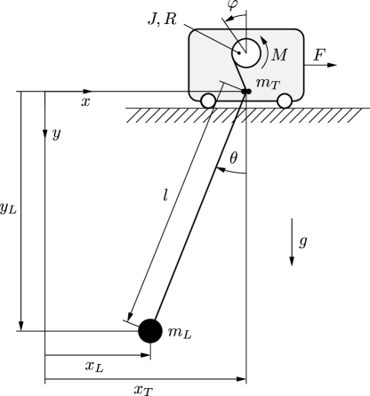
In Fig. 1, the schematic model of the considered gantry crane is shown. The position of the trolley is denoted by $x_{T}$, the rotation angle of the rope drum is denoted by $\varphi$, and $\theta$ describes the pendulum angle. With the length of the rope $l=R\varphi$, the position of the load is given by $x_{L}=x_{T}-R\varphi\sin(\theta)$ and $y_{L}=R\varphi\cos(\theta)$. The mass of the trolley is denoted by $m_{T}$, and $J$ represents the moment of inertia of the rope drum. The load has the mass $m_{L}$, and the gravitational acceleration $g$ points in the positive $y$-direction. The driving force $F$ which acts on the trolley and the driving torque $M$ which acts on the rope drum are the control inputs. The equations of motion can be found e.g. in [11] and read as

$$\begin{aligned} (m_{T}+m_{L})\ddot{x}_{T}-m_{L}R\sin(\theta)\ddot{\varphi}-m_{L}R\varphi\cos(\theta)\ddot{\theta}\;\\ +m_{L}\dot{\theta}(R\varphi\dot{\theta}\sin(\theta)-2R\dot{\varphi}\cos(\theta))&=F\,,\\ -m_{L}R\sin(\theta)\ddot{x}_{T}+(J+m_{L}R^{2})\ddot{\varphi}\;\\ -m_{L}R(R\varphi\dot{\theta}^{2}+g\cos(\theta))&=M\,,\\ -\cos(\theta)\ddot{x}_{T}+R\varphi\ddot{\theta}+2R\dot{\varphi}\dot{\theta}+g\sin(\theta)&=0\,.\end{aligned}$$

A state representation (1) is given by

$$\begin{aligned} \dot{x}_{T}&=v_{T}\\ \dot{\varphi}&=\omega_{\varphi}\\ \dot{\theta}&=\omega_{\theta}\\ \text{$\dot{v}_{T}$}&=f_{a_{T}}(\varphi,\theta,\omega_{\theta},F,M)\\ \dot{\omega}_{\varphi}&=f_{\alpha_{\varphi}}(\varphi,\theta,\omega_{\theta},F,M)\\ \dot{\omega}_{\theta}&=f_{\alpha_{\theta}}(\varphi,\theta,\omega_{\varphi},\omega_{\theta},F,M)\end{aligned}$$ (10)

with the state $x=(x_{T},\varphi,\theta,v_{T},\omega_{\varphi},\omega_{\theta})$ and the input $u=(F,M)$. It is well-known that the model of the gantry crane is flat and that the position of the load is a flat output $y=(x_{T}-R\varphi\sin(\theta),R\varphi\cos(\theta))$. In order to derive a sampled-data model, in a first attempt one may simply compute the Euler-discretization of (10). However, it can be shown that the resulting discrete-time system does not meet the necessary conditions given in [12] and is thus not forward-flat. In fact, the test for forward-flatness stated in [13] fails already in the second step. Thus, we follow the approach suggested in Section 2.2 and search for a state- and input transformation (9) that transforms (10) into a structurally flat triangular representation (6). It turns out that for the gantry crane such a transformation indeed exists. A suitable state transformation is given by

$$\begin{aligned} x_{L}&=x_{T}-R\varphi\sin(\theta)\\ y_{L}&=R\varphi\cos(\theta)\\ v_{L,x}&=v_{T}-\omega_{\varphi}R\sin(\theta)-\omega_{\theta}R\varphi\cos(\theta)\\ v_{L,y}&=R(\omega_{\varphi}\cos(\theta)-\sin(\theta)\varphi\omega_{\theta})\,,\end{aligned}$$ (11)

where the transformed state $\bar{x}=(x_{L},y_{L},v_{L,x},v_{L,y},\theta,\omega_{\theta})$ contains the flat output and its first time derivative. In such coordinates, the system equations read as

$$\begin{aligned} \dot{x}_{L}&=v_{L,x}\\ \dot{y}_{L}&=v_{L,y}\\ \text{$\dot{\theta}$}&=\omega_{\theta}\\ \dot{v}_{L,x}&=f_{a_{L,x}}(y_{L},\theta,\omega_{\theta},M)\\ \dot{v}_{L,y}&=f_{a_{L,y}}(y_{L},\theta,\omega_{\theta},M)\\ \dot{\omega}_{\theta}&=f_{\alpha_{\theta}}(v_{L,y},\theta,\omega_{\theta},F,M)\,.\end{aligned}$$ (12)

If we additionally introduce the new input $\bar{u}=(a_{L,x},\alpha_{\theta})$ defined by

$$\begin{aligned} \begin{aligned} a_{L,x}&=f_{a_{L,x}}(y_{L},\theta,\omega_{\theta},M)\\ \alpha_{\theta}&=f_{\alpha_{\theta}}(v_{L,y},\theta,\omega_{\theta},F,M)\,,\end{aligned}\end{aligned}$$

i.e., the acceleration $a_{L,x}$ of the load in $x$-direction and the angular acceleration $\alpha_{\theta}$, we obtain a structurally flat triangular representation

$$\dot{x}_{L} =v_{L,x}$$ (13)

$$\dot{y}_{L} =v_{L,y}$$

$$\dot{v}_{L,x} =a_{L,x}$$

$$\dot{v}_{L,y} =g-\tfrac{a_{L,x}}{\tan(\theta)}$$

$$\text{$\dot{\theta}$} =\omega_{\theta}$$

$$\dot{\omega}_{\theta} =\alpha_{\theta}$$

with the flat output $y=(x_{L},y_{L})$. Due to the triangular structure the Euler-discretization of (13) is forward-flat (see Theorem 1), and because of Corollary 1 the same applies to the Euler-discretization of (12) with the original inputs $(F,M)$ given by

$$\begin{aligned} x_{L}^{+}&=x_{L}+T_{s}v_{L,x}\\ y_{L}^{+}&=y_{L}+T_{s}v_{L,y}\\ \text{$\theta^{+}$}&=\theta+T_{s}\omega_{\theta}\\ v_{L,x}^{+}&=v_{L,x}+T_{s}f_{a_{L,x}}(y_{L},\theta,\omega_{\theta},M)\\ v_{L,y}^{+}&=v_{L,y}+T_{s}f_{a_{L,y}}(y_{L},\theta,\omega_{\theta},M)\\ \omega_{\theta}^{+}&=\omega_{\theta}+T_{s}f_{\alpha_{\theta}}(v_{L,y},\theta,\omega_{\theta},F,M)\,.\end{aligned}$$ (14)

The corresponding parameterizing map (4) is of the form

$$\begin{aligned} \bar{x}&=F_{\bar{x}}(x_{L},y_{L},\dots,x_{L,[3]},y_{L,[3]})\\ u&=F_{u}(x_{L},y_{L},\dots,x_{L,[4]},y_{L,[4]})\end{aligned}$$ (15)

and will be used in the next section for the design of two different tracking controllers. For simplicity, in the remainder of the paper the bar-notation will be omitted.

3 Discrete-time Flatness-based Tracking Control

The design of a continuous-time flatness-based tracking control is typically divided into two steps. First, the system is exactly linearized by either an endogenous dynamic feedback or a quasi-static state feedback, see e.g. [2] and [10]. Subsequently, a further feedback is applied in order to stabilize reference trajectories. However, since the resulting control law is assumed to be evaluated continuously, it actually cannot be realized on a digital computer/processor with only a finite sampling rate. Nevertheless, for applications where the sampling rate can be chosen sufficiently high, a discrete-time evaluation of the control law usually leads to satisfying results.

In this section, however, we propose an alternative approach and design flatness-based tracking controllers directly for the sampled-data model (14) of the gantry crane. Like in the continuous-time case, we follow the two-step design philosophy with an exact linearization and a subsequent stabilizing feedback. For the exact linearization we use two different approaches based on a dynamic as well as a quasi-static state feedback. Furthermore, we demonstrate how the controllers can be extended by integral parts in order to compensate for stationary deviations caused e.g. by model uncertainties.

3.1 Tracking control with linearization by endogenous dynamic feedback

In [8], we have shown that discrete-time flat systems (including both forward- and backward shifts) can be linearized by a certain class of dynamic feedback

$$\begin{aligned} z^{+}&=\alpha(x,z,v)\\ u&=\beta(x,z,v)\end{aligned}$$

that closely mimics the class of endogenous dynamic feedback from the continuous-time case. In the following, we demonstrate the construction of such a linearizing dynamic feedback as well as an additional feedback to stabilize reference trajectories.

First, we extend the parameterizing map (4) by a map $z=F_{z}(y,\dots,y_{[r-1]})$ with $\dim(z)=\sum_{j=1}^{m}r_{j}-n$, such that the combined map $F_{xz}=(F_{x},F_{z})$ has a regular Jacobian matrix and is hence invertible. Since $F_{x}$ is a submersion, such an extension always exists. Next, we define the map $\Phi(y,\dots,y_{[r]})$ given by

$$x =F_{x}(y,\dots,y_{[r-1]})$$ (16)

$$z =F_{z}(y,\dots,y_{[r-1]})$$

$$v =y_{[r]}$$

and its inverse $\hat{\Phi}(x,z,v)$ given by

$$\begin{array}[]{c}\begin{aligned} (y,\dots,y_{[r-1]})&=\hat{F}_{xz}(x,z)\\ y_{[r]}&=v\,.\end{aligned}\end{array}$$ (18)

As shown in [8], a linearizing dynamic feedback follows by evaluating

$$\begin{aligned} z^{+}&=\delta_{y}(F_{z})\circ\hat{\Phi}(x,z,v)\\ u&=F_{u}\circ\hat{\Phi}(x,z,v)\,.\end{aligned}$$ (19)

The state- and input transformation (18) would transform the closed-loop

$$\begin{aligned} x^{+}&=f(x,F_{u}\circ\hat{\Phi}(x,z,v))\\ z^{+}&=\delta_{y}(F_{z})\circ\hat{\Phi}(x,z,v)\end{aligned}$$

into Brunovsky normal form $y_{[r_{j}]}^{j}=v^{j}$ for $j=1,\dots,m$. In such coordinates, a tracking controller for a reference trajectory $y_{d}(k)$ can now be designed easily. For this purpose, we introduce the tracking error and its forward-shifts as

$$e_{[i]}^{j}=y_{[i]}^{j}-y_{d,[i]}^{j}\,,\hphantom{a}j=1,\dots,m\,.$$ (20)

In order to stabilize a reference trajectory we use a linear tracking error dynamics of the form

$$e_{[r_{j}]}^{j}+\sum_{i=0}^{r_{j}-1}a_{i}^{j}e_{[i]}^{j}=0\,,\hphantom{a}j=1,\dots,m\,,$$ (21)

where the coefficients $a_{i}^{j}$ are chosen such that the roots of (21) are located within the unit circle. By substituting the definition (20) of the tracking error into (21) and solving for $y_{[r_{j}]}=v$, the stabilizing feedback for the new input $v$ follows as

$$v^{j}=y_{d,[r_{j}]}^{j}-\sum_{i=0}^{r_{j}-1}a_{i}^{j}(y_{[i]}^{j}-y_{d,[i]}^{j})\,,\hphantom{a}j=1,\dots,m\,.$$ (22)

In a last step, we have to express the forward-shifts of the flat output that appear in (22) by the system state $x$ and the controller state $z$. By substituting $(y,\dots,y_{[r-1]})=\hat{F}_{xz}(x,z)$ according to the map (18) into (22) and subsequently (22) into (19), the complete control law follows as

$$\begin{aligned} z^{+}&=\zeta(x,z,y_{d},\dots,y_{d,[r]})\\ u&=\eta(x,z,y_{d},\dots,y_{d,[r]})\,.\end{aligned}$$

It depends on the state $x$ of the system (3), the controller state $z$, and the reference trajectory $y_{d}$ as well as its forward-shifts. Thus, for a practical implementation, the state $x$ has to be measured or estimated by an observer.

For the sampled-data model (14) of the gantry crane, a linearizing dynamic feedback (19) can be constructed by choosing $F_{z}$ of (16) as

$$z^{1} =y_{L,[2]}$$

$$z^{2} =y_{L,[3]}\,.$$

The order of the resulting tracking error dynamics (21) is given by $r=(4,4)$. As we show in the next section, a lower order can be achieved by a linearization with a quasi-static feedback.

3.2 Tracking control with linearization by quasi-static state feedback

In [10], it is shown that every flat continuous-time system can be linearized by a quasi-static state feedback. In contrast to the linearization by dynamic feedback, the resulting control law is static but involves time derivatives of the closed-loop input. Despite these time derivatives of the new input, the approach is very useful for the design of flatness-based tracking controls. The main advantage over designs with dynamic feedback linearization is that it leads to lower order tracking error dynamics. In the following, we transfer this idea to discrete-time systems and design a tracking control based on a linearization by a discrete-time quasi-static state feedback for the sampled-data model (14) of the gantry crane.

The exact linearization of flat systems by quasi-static feedback discussed in [10] is based on the concept of generalized state representations. According to [20], for discrete-time systems generalized state representations are of the form

$$\tilde{x}^{+}=f(\tilde{x},u,u_{[1]},\dots,u_{[\gamma]})$$

and can also depend on forward-shifts of the input (instead of time derivatives in the continuous-time case). Such a generalized system representation follows from (3) by a generalized state transformation of the form

$$\tilde{x}=\Psi_{x}(x,u,u_{[1]},\dots,u_{[\nu]})$$ (23)

with $\textrm{rank}(\partial_{x}\Psi_{x})=n$. The rank condition ensures that the generalized state transformation (23) is invertible. For the class of forward-flat systems, it can be shown that there always exist generalized states of the form

$$\tilde{x}_{B}=(y^{1},y_{[1]}^{1},\dots,y_{[\kappa_{1}-1]},\dots,y^{m},y_{[1]}^{m},\dots,y_{[\kappa_{m}-1]}^{m})$$ (24)

which consist of the components of the flat output and its forward-shifts up to some order $\kappa-1=(\kappa_{1}-1,\dots,\kappa_{m}-1)$ with $\dim(\tilde{x}_{B})=n$ and $\kappa_{j}\leq r_{j}$. In accordance with the continuous-time case [10], we call (24) a generalized Brunovsky state. With a feedback of the form

$$u=F_{u}(\tilde{x}_{B},v,v_{[1]},\dots,v_{[r-\kappa]})\,,$$ (25)

which is constructed by replacing the $n$ components of $y,\dots,y_{[\kappa-1]}$ in the map $F_{u}$ of (4) with the Brunovsky state $\tilde{x}_{B}$ and the remaining components $y_{[\kappa]},\dots,y_{[r]}$ with the new input and its forward-shifts $v,\dots,v_{[r-\kappa]}$, we get an input/output behaviour of the form

$$y_{[\kappa_{j}]}^{j}=v^{j}\,,\hphantom{a}j=1,\dots,m\,.$$ (26)

In the continuous-time case discussed in [10], such a feedback is called a quasi-static state feedback. With the linear input/output behaviour (26), it is now easy to construct a further feedback in order to introduce e.g. a linear tracking error dynamics

$$e_{[\kappa_{j}]}^{j}+\sum_{i=0}^{\kappa_{j}-1}a_{i}^{j}e_{[i]}^{j}=0\,,\hphantom{a}j=1,\dots,m\,.$$ (27)

The coefficients $a_{i}^{j}$ must be chosen such that the roots of (27) are located within the unit circle. By substituting the definition (20) of the tracking error into (27) and solving for $y_{[\kappa_{j}]}=v$, the stabilizing feedback follows as

$$v^{j}=y_{d,[\kappa_{j}]}^{j}-\sum_{i=0}^{\kappa_{j}-1}a_{i}^{j}(y_{[i]}^{j}-y_{d,[i]}^{j})\,,\hphantom{a}j=1,\dots,m\,.$$

The forward-shifts of $v$ that are required for the quasi-static feedback (25) follow as

$$v_{[p]}^{j}=y_{d,[\kappa_{j}+p]}^{j}-\sum_{i=0}^{\kappa_{j}-1}a_{i}^{j}(y_{[i+p]}^{j}-y_{d,[i+p]}^{j})$$

for $p=1,\dots,r_{j}-\kappa_{j}$. With the relation $v_{[p]}^{j}=y_{[\kappa_{j}+p]}^{j}$, which is a consequence of (26), we get the set of linear equations

$$\begin{aligned} v^{j}&=y_{d,[\kappa_{j}]}^{j}-\sum_{i=0}^{\kappa_{j}-1}a_{i}^{j}(y_{[i]}^{j}-y_{d,[i]}^{j})\\ v_{[1]}^{j}&=y_{d,[\kappa_{j}+1]}^{j}-a_{\kappa_{j}-1}^{j}(v^{j}-y_{d,[\kappa_{j}]}^{j})-\sum_{i=0}^{\kappa_{j}-2}a_{i}^{j}(y_{[i+1]}^{j}-y_{d,[i+1]}^{j})\\ &\vdots\\ v_{[r_{j}-\kappa_{j}]}^{j}&=\ldots\end{aligned}$$ (28)

$j=1,\dots,m$ for $v,\dots,v_{[r-\kappa]}$. One could now solve (28) for $v,\dots,v_{[r-\kappa]}$ systematically from top to bottom and insert the solution into (25). However, the resulting control law would depend on the generalized Brunovsky state (24), i.e., on forward-shifts of the flat output up to order $\kappa-1$. Since future values of the flat output can in general not be measured, the resulting control law is obviously difficult to implement. Thus, we try to replace the flat output and its forward-shifts beforehand, which is possible if two assumptions are met. First, we assume that with

$$x=F_{x}(\tilde{x}_{B},v,v_{[1]},\dots,v_{[r-\kappa-1]})\,,$$

where we have inserted (24) as well as (26) and its forward-shifts into the map $F_{x}$ of (4), the condition $\textrm{$\mathrm{rank}$}(\partial_{\tilde{x}_{B}}F_{x})=n$ is met. This guarantees by the implicit function theorem that the Brunovsky state can be expressed as

$$\tilde{x}_{B}=\phi(x,v,v_{[1]},\dots,v_{[r-\kappa-1]})\,.$$ (29)

Substituting (29) into (25) yields the linearizing feedback

$$u=F_{u}(\phi(x,v,v_{[1]},\dots,v_{[r-\kappa-1]}),v,v_{[1]},\dots,v_{[r-\kappa]})\,,$$ (30)

which introduces the same input/output behaviour (26) as (25) but depends on $x$ instead of $\tilde{x}_{B}$. However, we also have to determine $v,v_{[1]},\dots,v_{[r-\kappa]}$ as a function of $x$ instead of $\tilde{x}_{B}$. For this purpose, we substitute (29) into (28) and obtain a set of in general nonlinear equations. Thus, our second assumption is that this set of nonlinear equations can nevertheless be solved for $v,\dots,v_{[r-\kappa]}$, i.e.,

$$(v,v_{[1]},\dots,v_{[r-\kappa]})=\chi(x,y_{d},\dots,y_{d,[r]})\,.$$ (31)

Finally, by substituting (31) into (30), we obtain a static control law of the form

$$u=\eta(x,y_{d},\dots,y_{d,[r]})\,,$$ (32)

which only depends on the state $x$ as well as the reference trajectory $y_{d}$ and its forward-shifts. Thus, like for the dynamic tracking controller of Section 3.1, only the state $x$ is required for an implementation.

For the sampled-data model (14) of the gantry crane, a generalized Brunovsky state (24) is given by

$$\tilde{x}_{B}=(x_{L},\dots,x_{L,[3]},y_{L},y_{L,[1]})\,.$$

Since both above assumptions are met, a control law of the form (32) can be derived. Compared to the dynamic controller of Section 3.1, the order of the resulting tracking error dynamics (27) is reduced to $\kappa=(4,2)$.

3.3 Extension of the tracking error dynamics by integral parts

In this section, we show how the discrete-time tracking control with dynamic feedback of Section 3.1 can be extended by discrete-time integral parts in order to avoid stationary errors caused e.g. by model uncertainties. In the case of the gantry crane, such errors occur mainly due to friction effects. With the “integrated” tracking error $e_{I}$ given by

$$e_{I}^{j,+}=e_{I}^{j}+T_{s}e^{j}\,,\hphantom{a}j=1,\dots,m\,,$$

the extended error dynamics reads as

$$\left[\begin{array}[]{c}e_{I}^{j,+}\\ e^{j,+}\\ \vdots\\ e_{[r_{j}-1]}^{j,+}\end{array}\right]=\underset{A^{j}}{\underbrace{\left[\begin{array}[]{ccccc}1&T_{s}&0&0&0\\ 0&0&1&\ddots&0\\ \vdots&\vdots&\ddots&\ddots&0\\ 0&0&\cdots&0&1\\ -a_{I}^{j}&-a_{0}^{j}&\cdots&\cdots&-a_{r_{j}-1}^{j}\end{array}\right]}}\left[\begin{array}[]{c}e_{I}^{j}\\ e^{j}\\ \vdots\\ e_{[r_{j}-1]}^{j}\end{array}\right]\,,$$

$j=1,\dots,m$. To obtain a stable error dynamics, the coefficients $a_{I}^{j}$ and $a_{i}^{j}$ must be chosen such that all eigenvalues of the matrices $A^{j}$ are located within the unit circle. The extended stabilizing feedback for the exactly linearized system follows as

$$\bar{v}^{j}=v^{j}-a_{I}^{j}e_{I}^{j}\,,\hphantom{a}j=1,\dots,m\,,$$

where $v$ represents the feedback without integral parts obtained in Section 3.1. For the controller with quasi-static state feedback of Section 3.2, an extension by integral parts is possible in a similar way. With respect to the gantry crane, the integral parts increase the order of the error dynamics to $(5,5)$ for the dynamic controller and $(5,3)$ for the quasi-static controller.

4 Trajectory Planning and Measurement Results

Figure 2: Laboratory model of the gantry crane.

In the following, we present measurement results for the novel discrete-time quasi-static controller of Section 3.2, which was implemented on a laboratory model of the gantry crane depicted in Fig. 2. In particular, in Section 4.1 we compare its tracking performance for different sampling rates with the continuous-time quasi-static tracking controller discussed in [11]. Moreover, in Section 4.2 we show how the discrete-time approach facilitates the design of optimal reference trajectories. We formulate and solve an optimization problem and present measurement results for the computed trajectories. Finally, in Section 4.3 we show further measurement results for the tracking of a closed path.

Like in [11], for all experiments the control law (32) is extended by a feedforward compensation

$$\begin{aligned} F_{fr,d}&=r_{v,T}v_{T,d}+r_{C,T}\textrm{sign}(v_{T,d})\\ M_{fr,d}&=r_{v,\varphi}\omega_{\varphi,d}+r_{C,\varphi}\textrm{sign}(\omega_{\varphi,d})\end{aligned}$$ (33)

of the friction in order to improve the tracking behaviour. The required reference trajectories for the velocity of the trolley $v_{T}$ and the angular velocity $\omega_{\varphi}$ of the rope drum can be computed from the reference trajectories of the flat output $y=(x_{L},y_{L})$ by the inverse of the state transformation (11) and the parameterizing map (15). The friction compensation (33) is simply added to the values of the control inputs $F$ and $M$ determined by the tracking control law (32) derived in Section 3.2. Like in [11], we use an asymmetric friction compensation, i.e., the friction coefficients depend on the sign of the velocities $v_{T,d}$ and $\omega_{\varphi,d}$. In addition to the compensation of the friction, we also use integral parts (cf. Section 3.3) to avoid steady-state control deviations. As it is common practice for continuous-time systems, these integral parts are activated only at the end of the transitions, i.e., after the reference trajectory has already reached the final desired position.

4.1 Comparison continuous-time and discrete-time flatness-based control

In this section, we compare the tracking performance of the discrete-time quasi-static controller designed in Section 3.2 with the continuous-time quasi-static controller of [11]. For this purpose, as a benchmark, we use a transition of the load from the rest position $y_{d,0}=(0.2\,\textrm{m},0.7\,\textrm{m})$ to the rest position $y_{d,T}=(1.0\,\textrm{m},0.5\,\textrm{m})$ in a transition time of $T=1.7\,\textrm{s}$. Before presenting measurement results, we briefly discuss the design of the reference trajectories in the continuous-time as well as in the discrete-time case.

In general, a continuous-time flatness-based control law involves not only the reference trajectory $y_{d}(t)$ itself but also its time derivatives. Hence, the trajectory needs to be sufficiently often differentiable. Since we transfer the load between two rest positions, it must satisfy the initial- and final conditions

$$y_{d}^{j}(0)=y_{d,0}^{j}\,,\hphantom{aa}y_{d}^{j}(T)=y_{d,T}^{j}$$ (34)

and

$$\tfrac{d^{i}}{dt^{i}}y_{d}^{j}(t)\bigg{|}_{t=0}=\tfrac{d^{i}}{dt^{i}}y_{d}^{j}(t)\bigg{|}_{t=T} =0$$ (35)

for $i=1,\dots,r_{j}-1$ and $j=1,\dots,m$. For the gantry crane, we have both for the $x$- and the $y$-direction four conditions at $t=0$ as well as four conditions at $t=T$. Thus, the simplest approach are polynomial trajectories

$$\begin{aligned} x_{L,d}(t)&=\sum_{i=0}^{7}c_{x,i}t^{i}\\ y_{L,d}(t)&=\sum_{i=0}^{7}c_{y,i}t^{i}\end{aligned}$$ (36)

of order seven with suitably chosen coefficients $c_{x,i}$ and $c_{y,i}$.

In the discrete-time case, the control law (32) depends on the desired sequence $y_{d}(k)$ and its forward-shifts. In contrast to the continuous-time case, differentiability is not required. However, since we want to achieve a transition between rest positions, the reference trajectory needs to satisfy the conditions

$$\begin{aligned} y_{d}^{j}(0)&=\ldots=y_{d}^{j}(r_{j}-1)=y_{d,0}^{j}\\ y_{d}^{j}(N)&=\ldots=y_{d}^{j}(N+r_{j}-1)=y_{d,T}^{j}\end{aligned}$$ (37)

for $j=1,\dots,m$ with $T=NT_{s}$, which are the discrete-time counterpart to (34) and (35). Thus, in principle, for the gantry crane we could again use a polynomial ansatz of order $(7,7)$. However, in the following we simply evaluate the continuous-time reference trajectory at the time instants $t=kT_{s}$. Since (36) is used to connect rest positions, the conditions (37) are obviously satisfied.

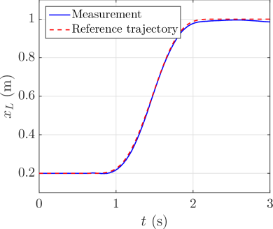
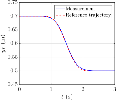
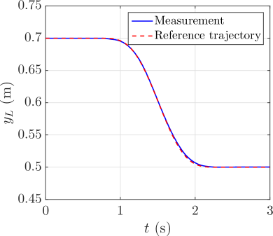
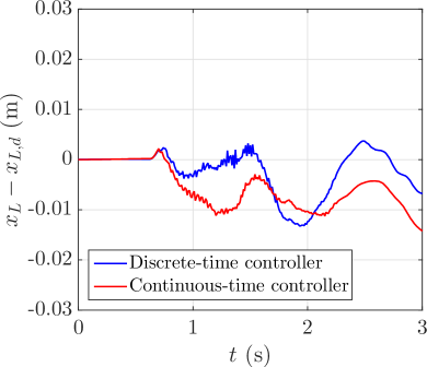
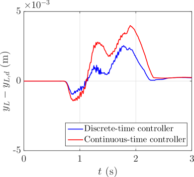
Both the continuous-time and the discrete-time tracking controller have been implemented on a dSPACE^® real-time system with different sampling times $T_{s}$. The continous-time control law of [11] is simply evaluated at the time instants $t=kT_{s}$. In the first experiment, we compare both controllers without integral parts and a sampling time of $T_{s}=10\,\textrm{ms}$. The corresponding measurements are shown in Fig. 3 and Fig. 4. It can be observed that with both controllers the reference trajectory is almost perfectly tracked. Fig. 5 shows the corresponding tracking errors. The small deviations and stationary errors are caused mainly by the non-ideal compensation of the friction.

Figure 3: Tracking performance of the continuous-time flatness-based controller ($T_{s}=10\,\textrm{ms}$).

Figure 4: Tracking performance of the discrete-time flatness-based controller ($T_{s}=10\,\textrm{ms}$).

Figure 5: Tracking error comparison ($T_{s}=10\,\textrm{ms}$).

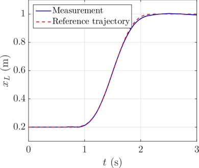
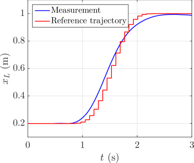
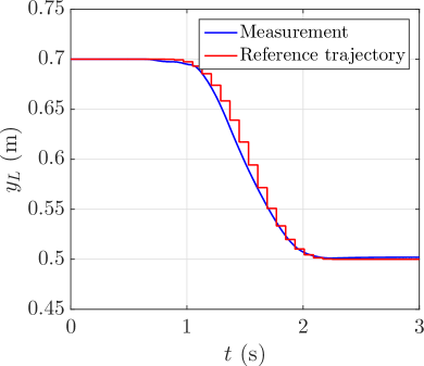
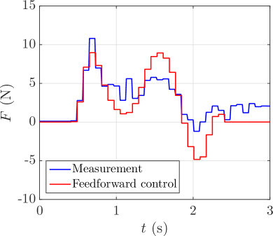
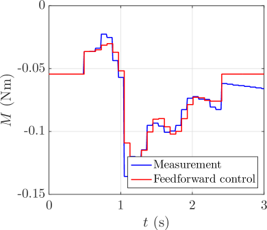
In the second experiment, the sampling time is increased to $T_{s}=80\,\textrm{ms}$. It turns out that this sampling time is too large for the continuous-time controller, whereas the discrete-time controller still transfers the load between the rest positions as desired. The corresponding measurements are shown in Fig. 6. However, it can be observed that the reference trajectory is no longer tracked that well. The reason is that the Euler-discretization is not exact and the approximation error increases with the sampling time. Nevertheless, the novel discrete-time controller seems to be quite robust with respect to high sampling times (as further experiments up to $T_{s}=100\,\textrm{ms}$ have shown). In Fig. 7, both the actual control inputs as well as the pure feedforward part (including the friction compensation) of the control law are depicted. It can be seen that at the end of the transition both inputs do not exactly have the expected stationary values. This is due to the steady-state deviation caused by static friction and will be discussed in more detail in the next section.

Figure 6: Tracking performance of the discrete-time flatness-based controller ($T_{s}=80\,\textrm{ms}$).

Figure 7: Actual control inputs and feedforward part ($T_{s}=80\,\textrm{ms}$).

4.2 Design of reference trajectories by optimization

In the following, we use the flatness of the gantry crane to design reference trajectories that minimize a given objective function. Instead of searching for state- and input trajectories, which are constrained by the system equations, we formulate the optimization problem in terms of the flat output. As it is well-known, the advantage of the latter approach is that the trajectories of the flat output are free and the system equations do not need to be taken into account as constraints. In the continuous-time case, the possible trajectories of the flat output belong to an infinite-dimensional space. Thus, in order to get a finite-dimensional optimization problem, the trajectories are usually restricted to a set of functions described by a finite number of parameters, see e.g. [22]. Possible approaches are the use of spline curves or the method applied in [11]. In the discrete-time case, in contrast, the optimization problem is inherently finite-dimensional since we are dealing with sequences instead of functions.

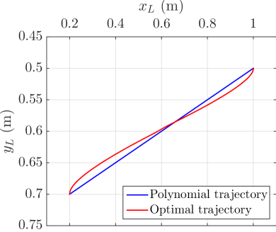
In the following, we formulate and solve such an optimization problem for the sampled-data model (14) of the gantry crane. The goal is to achieve a transition between the two rest positions of Section 4.1 in $T=3\,\textrm{s}$ while minimizing the absolute acceleration

$$a_{L}=\sqrt{f_{a_{L,x}}^{2}+f_{a_{L,y}}^{2}}$$

of the load. The functions $f_{a_{L,x}}$ and $f_{a_{L,y}}$ are the same as in (12). By the use of the parameterizing map (15), $a_{L}$ can now be expressed as a function of the flat output and its forward-shifts. The optimization problem can be formulated as

$$\begin{aligned} \underset{p}{\textrm{$\mathrm{min}$}}&\,\text{$\varepsilon$}\\ \text{$\mathrm{s.t.}$}\,&a_{L}(k)\leq\varepsilon\\ &|F(k)|\leq F_{\textrm{max}}\\ &|M(k)|\leq M_{\textrm{max}}\end{aligned}$$

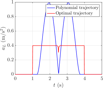
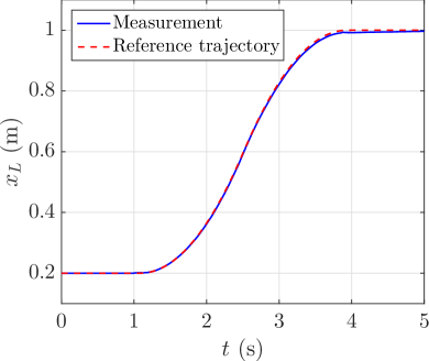
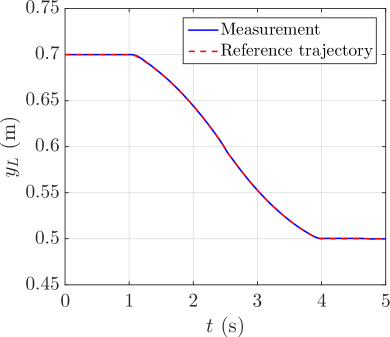
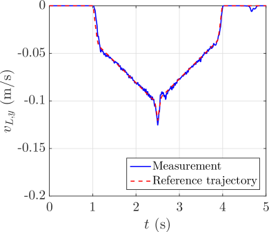
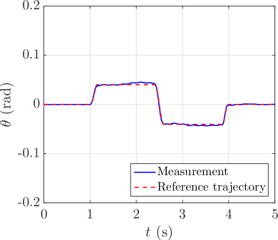
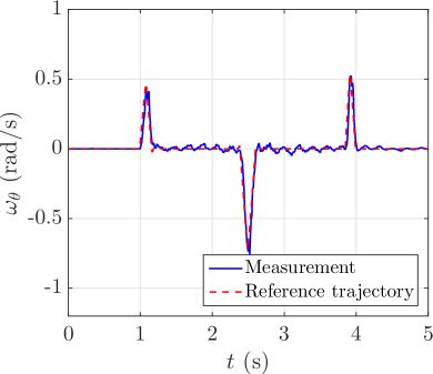
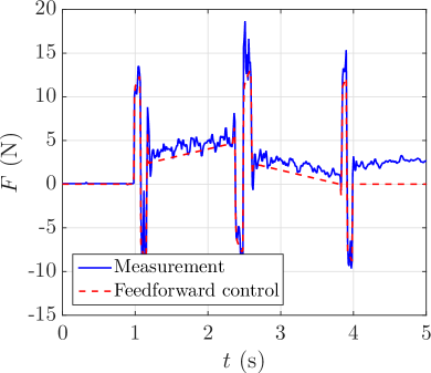
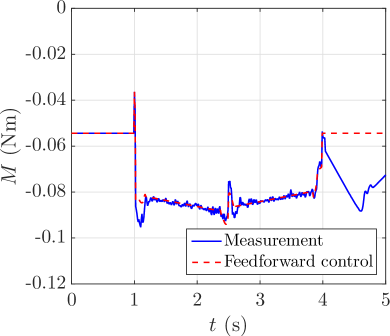
with $k=0,\dots,N-1$. The inputs have been limited by $F_{\textrm{max}}=10\,\text{N}$ and $M_{\textrm{max}}=0.2\,\textrm{Nm}$. Since the load shall be transferred from one rest position to another, the reference trajectory needs to satisfy the conditions (37) and the vector of optimization variables is reduced to $p=[\varepsilon,y_{d}(4),\dots,y_{d}(N-1)]$. In Fig. 8, the calculated optimal trajectory for a sampling time of $T_{s}=10\,\textrm{ms}$ as well as the polynomial trajectory, which was used as initial value for the optimization, are shown. The absolute value $a_{L}$ of the acceleration of the load is shown in Fig. 9 for both the polynomial as well as the optimized trajectory. It can be observed that for the optimal trajectory the acceleration is constant during almost the whole transition. The corresponding input trajectory $F(k)$ temporarily reaches the limits $\pm F_{\text{max}}$ at the beginning, in the middle, and at the end of the transition, while the constraint $|M(k)|\leq M_{\textrm{max}}$ is never active.

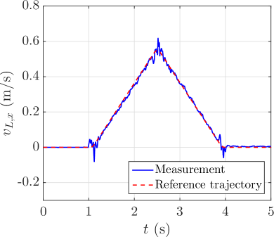
Figures 10 to 13 show measurement results for the determined optimal trajectory. In Fig. 10, it can be observed that the reference trajectories are again almost perfectly tracked. Particularly interesting are the horizontal and vertical velocities of the load depicted in Fig. 11, which increase and decrease for most of the time with a constant slope. This is in accordance with the almost constant acceleration of Fig. 9. The corresponding control inputs are shown in Fig. 13. It can be seen that because of the additional friction compensation already the feedforward part slightly exceeds the limit $|F(k)|\leq F_{\textrm{max}}$. However, the resulting control input, including the feedback part, remains within the input limitations of the laboratory setup. At the end of the transition at $t=4\,\textrm{s}$, it can again be observed that the inputs $F$ and $M$ do not exactly have the expected stationary values because the end position of the load slightly differs from its desired position. Thus, the controller attempts to compensate this error. Since the resulting force $F$ and torque $M$ are too small to overcome the static friction of the trolley and the rope drum, these input values would be applied permanently. For this experiment, however, we have used the extended control law with integral parts, which are activated after the transition of the reference trajectory is completed. Consequently, as can be observed in Fig. 13, the applied inputs increase after $t=4\,\textrm{s}$ until they are large enough to overcome the static friction.

Figure 8: Optimal trajectory ($T_{s}=10\,\textrm{ms}$).

Figure 9: Acceleration for the optimal trajectory ($T_{s}=10\,\textrm{ms}$).

Figure 10: Position tracking performance for the optimal trajectory ($T_{s}=10\,\textrm{ms}$).

Figure 11: Velocity tracking performance for the optimal trajectory ($T_{s}=10\,\textrm{ms}$).

Figure 12: Angle and angular velocity tracking performance for the optimal trajectory ($T_{s}=10\,\textrm{ms}$).

Figure 13: Actual control inputs and feedforward part for the optimal trajectory ($T_{s}=10\,\textrm{ms}$).

4.3 Tracking a closed path

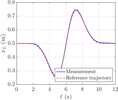
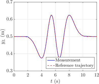
As already mentioned in Section 4.1, in the continuous-time case the reference trajectory $y_{d}(t)$ needs to be sufficiently often differentiable. Moreover, in order to track a reference trajectory $y_{d}(t)$, all time derivatives up to $y_{d}^{(r)}(t)$ must be computed beforehand. In the discrete-time case, in contrast, there are no restrictions on the reference trajectory $y_{d}(k)$ such as differentiability, and instead of time derivatives the control law involves only forward-shifts of $y_{d}(k)$. This simplifies the implementation, since these forward-shifts can be constructed easily by chains of unit delays.

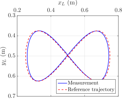
To show the flexibility of the discrete-time approach, in the last experiment a closed path with the shape of a lying eight is used as reference trajectory. In Fig. 14, it can be seen that $y_{d}(k)$ is tracked well and that the stationary errors at the end of the reference trajectory are compensated by the integral parts. Fig. 15 shows the desired and the measured trajectory in the $xy$-plane. The small deviations at the reversal points of the load are caused by the strong friction of the trolley on the rail.

Figure 14: Position tracking performance for a closed path ($T_{s}=10\,\textrm{ms}$).

Figure 15: Tracking a closed path ($T_{s}=10\,\textrm{ms}$).

5 Conclusion

We have shown by means of the laboratory model of a gantry crane that the concept of discrete-time flatness is well-suited for the design of tracking controllers in practical applications. For nonlinear systems, the difficulty lies in determining a flat sampled-data model of the plant. In order to overcome this problem, we have proposed a constructive method which relies on a combination of a suitable state transformation and a subsequent Euler-discretization. Although the Euler-discretization is not exact, experiments with the gantry crane have shown that the novel discrete-time flatness-based controller can be used over a significantly wider range of sampling rates than its continuous-time counterpart. Moreover, we have shown that the property of discrete-time flatness is also beneficial in the context of trajectory planning by optimization.

An important topic for future research are alternative, more precise discretization methods which also preserve the flatness. The goal is to achieve a better tracking performance for even lower sampling rates. In contrast to the proposed approach via the Euler-discretization, such methods may possibly lead to discrete-time systems which are flat in the more general sense of [8] and not necessarily forward-flat.

References

- [1] M. Fliess, J. Lévine, P. Martin, P. Rouchon, Sur les systèmes non linéaires différentiellement plats, Comptes rendus de l’Académie des sciences. Série I, Mathématique 315 (1992) 619–624.
- [2] M. Fliess, J. Lévine, P. Martin, P. Rouchon, Flatness and defect of non-linear systems: introductory theory and examples, International Journal of Control 61 (6) (1995) 1327–1361.
- [3] M. Fliess, J. Lévine, P. Martin, P. Rouchon, A Lie-Bäcklund approach to equivalence and flatness of nonlinear systems, IEEE Transactions on Automatic Control 44 (5) (1999) 922–937.
- [4] P. Kotyczka, T. Thoma, Symplectic discrete-time energy-based control for nonlinear mechanical systems, Automatica 133, (2021).
- [5] A. Kaldmäe, Ü. Kotta, On flatness of discrete-time nonlinear systems, in: Proceedings 9th IFAC Symposium on Nonlinear Control Systems, 2013, pp. 588–593.
- [6] B. Kolar, A. Kaldmäe, M. Schöberl, Ü. Kotta, K. Schlacher, Construction of flat outputs of nonlinear discrete-time systems in a geometric and an algebraic framework, IFAC-PapersOnLine (18) 796–801, 10th IFAC Symposium on Nonlinear Control Systems.
- [7] P. Guillot, G. Millérioux, Flatness and submersivity of discrete-time dynamical systems, IEEE Control Systems Letters 4 (2) (2020) 337–342.
- [8] J. Diwold, B. Kolar, M. Schöberl, A trajectory-based approach to discrete-time flatness, IEEE Control Systems Letters 6 (2022) 289–294.
- [9] H. Sira-Ramirez, S. Agrawal, Differentially Flat Systems, Marcel Dekker, New York, 2004.
- [10] E. Delaleau, J. Rudolph, Control of flat systems by quasi-static feedback of generalized states, International Journal of Control 71 (5) (1998) 745–765.
- [11] B. Kolar, H. Rams, K. Schlacher, Time-optimal flatness based control of a gantry crane, Control Engineering Practice 60 (2017) 18–27.
- [12] B. Kolar, M. Schöberl, J. Diwold, Differential-geometric decomposition of flat nonlinear discrete-time systems, Automatica 132, (2021).
- [13] B. Kolar, J. Diwold, M. Schöberl, Necessary and sufficient conditions for difference flatness, arXiv e-prints (2019) arXiv:1909.02868v2 [math.OC].
- [14] H. Nijmeijer, A. van der Schaft, Nonlinear Dynamical Control Systems, Springer, New York, 1990.
- [15] C. Gstöttner, B. Kolar, M. Schöberl, On a flat triangular form based on the extended chained form, IFAC-PapersOnLine 54 (9) (2021) 245–252, 24th International Symposium on Mathematical Theory of Networks and Systems.
- [16] C. Gstöttner, B. Kolar, M. Schöberl, A structurally flat triangular form based on the extended chained form, International Journal of Control (2020).
- [17] F. Nicolau, W. Respondek, Normal forms for multi-input flat systems of minimal differential weight, International Journal of Robust and Nonlinear Control 29 (10) (2019) 3139–3162.
- [18] F. Nicolau, W. Respondek, Normal forms for flat two-input control systems linearizable via a two-fold prolongation, IFAC-PapersOnLine 53 (2) (2020) 5441–5446, 21st IFAC World Congress.
- [19] J. Chiasson, A new approach to dynamic feedback linearization control of an induction motor, IEEE Transactions on Automatic Control 43 (1998) 391–397.
- [20] Ü. Kotta, Lowering the orders of input shifts in discrete-time generalized state-space systems, in: Proceedings 5th IFAC Conference on System Structure and Control, 1998, pp. 727–732.
- [21] E. Aranda-Bricaire, Ü. Kotta, Generalized controlled invariance for discrete-time nonlinear systems with an application to the dynamic disturbance decoupling problem, IEEE Transactions on Automatic Control 46 (1) (2001) 165–171.
- [22] P. Martin, R. Murray, P. Rouchon, Flat systems, in: G. Bastin, M. Gevers (Eds.), Plenary Lectures and Mini-Courses, Proceedings 4th European Control Conference (ECC), 1997, pp. 211–264.