TS-2021-0349

Luo, et al.

Efficient Algorithms for Stochastic Ride-pooling Assignment

Efficient Algorithms for Stochastic Ride-pooling Assignment with Mixed Fleets

Qi Luo Department of Industrial Engineering, Clemson University, Clemson, SC 29634 Viswanath Nagarajan Department of Industrial and Operations Engineering, University of Michigan, Ann Arbor, MI 48109 Alexander Sundt, Yafeng Yin Department of Civil and Environmental Engineering, University of Michigan, Ann Arbor, MI 48109 John Vincent, Mehrdad Shahabi Ford Motor Company, Dearborn, MI 48120

Ride-pooling, which accommodates multiple passenger requests in a single trip, has the potential to significantly increase fleet utilization in shared mobility platforms. The ride-pooling assignment problem finds optimal co-riders to maximize the total utility or profit on a shareability graph, a hypergraph representing the matching compatibility between available vehicles and pending requests. With mixed fleets due to the introduction of automated or premium vehicles, fleet sizing and relocation decisions should be made before the requests are revealed. Due to the immense size of the underlying shareability graph and demand uncertainty, it is impractical to use exact methods to calculate the optimal trip assignments. Two approximation algorithms for mid-capacity and high-capacity vehicles are proposed in this paper; the respective approximation ratios are $\frac{1}{p^{2}}$ and $\frac{e-1}{(2e+o(1))p\ln p}$, where $p$ is the maximum vehicle capacity plus one. The performance of these algorithms is validated using a mixed autonomy on-demand mobility simulator. These efficient algorithms serve as a stepping stone for a variety of multimodal and multiclass on-demand mobility applications.

ride-pooling assignment problem, approximation algorithm, mixed autonomy traffic

1 Introduction

Shared mobility fosters an ecosystem of connected travelers, disruptive vehicle technologies, and intelligent transportation infrastructure (Shaheen et al. 2017, Ke, Yang, and Zheng 2020). The platform aims to maximize vehicle fleet utilization by combining multiple requests into a single trip while minimizing the quality of service degradation. We term the process of assigning trip requests to available vehicles the ride-pooling assignment problem, a notion generalized from the ride-pooling option in ride-hailing services (Santi et al. 2014), whereas the underlying business model can vary from microtransit to shared autonomous vehicles. Efficient ride-pooling assignment algorithms must balance between maximizing the platform’s profits, improving the utility of passengers and drivers, and reducing total energy usage and emissions. Developing innovative ride-pooling assignment algorithms that meet the vast scales of customers and vehicles has been a significant research task in the burgeoning shared mobility industry.

When shared mobility applications migrate from the private to public sectors, the computational challenge of the ride-pooling assignment problem rises inevitably with the increasing vehicle capacity. Most heuristic methods focus on operating ride-pooling with at most two or three groups of customers (Santi et al. 2014, Ke et al. 2021, Erdmann, Dandl, and Bogenberger 2021, Sundt et al. 2021). Emerging shared mobility applications, such as microtransit, will operate high-capacity vehicle fleets (between 8 and 14 passengers per vehicle) and will necessitate more scalable algorithms (Markov et al. 2021, Hasan and Van Hentenryck 2021, Tafreshian et al. 2021). Per this study, a platform can benefit from operating mixed vehicle fleets to accommodate various customer preferences. However, including more types of services complicate fleet operations because of this uncertain customer preference. Now we introduce the Stochastic Ride-pooling Assignment with Mixed Fleets (SRAMF) problem that arises with the diversification of vehicle fleets in shared mobility platforms.

1.1 Overview of the SRAMF Problem

The SRAMF problem extends the scalable framework developed for the deterministic ride-pooling assignment for homogeneous fleets in Santi et al. (2014), Alonso-Mora et al. (2017). The main idea here is to decouple routing and trip-to-vehicle assignment into two sequential tasks based on the notion of “shareability graphs”. Given a batch of trip requests and available vehicles in each time interval, the procedure guarantees the anytime optimality (Alonso-Mora et al. 2017) such that the resulting ride-pooling assignments attain the exact optimal solution to the joint problem (see Appendix 8.1). The procedure is summarized as follows:

1. First, it constructs a shareability graph that describes the matchable relationship between all trip requests (demand) and available vehicles (supply) in each batch (see Figure 2) and compute the associated values of each route.

2. Next, the platform solves a general assignment problem (GAP) on this graph that maximizes the total matching value.

3. Finally, the shareability graph is updated by removing occupied vehicles and assigned demand and inserting arriving requests and available vehicles.

Our research focuses on the stochastic extension of the assignment problem (step 2 above). We defer the discussion on constructing shareability graphs (step 1 above) to Appendix 8. There, we describe a sequence of matching rules that can construct a hierarchical tree of matchable requests and significantly reduce the computational time. We show that the framework is computationally efficient and can be deployed with a rolling horizon with demand forecast (Yang et al. 2020) as well as varying time intervals (Qin et al. 2021).

While using the shareability graph can reduce the computational burden of solving dial-a-ride problems, deploying this framework with mixed fleets is nontrivial. Blending two or more types of vehicle fleets leads to new operational challenges due to uncertainty. SRAMF is a natural yet significant generalization of the ride-pooling assignment problem, which is motivated by the following applications:

Example 1: A platform provides several classes of mobility services for various market segments. For example, Uber operates a standard service (UberX) alongside a luxury service (Uber Black). In most instances, the platform tends to match customers with the requested vehicle class. However, if there are excessive demands in the standard class, it may be more advantageous for the platform to dispatch vehicles from the luxury class to the standard class to avoid reneging.

Example 2: A ride-hailing platform hires drivers as either permanent employees or freelancers (Dong et al. 2021). The platform pays a fixed hourly rate to its permanent employees and pays freelancers per finished trip. As a result, the platform needs to determine the priority of drivers in the ride-pooling assignment to facilitate the long-term hiring strategy for permanent employees.

Example 3: A shared mobility platform operates both fully automated vehicles (AVs) and conventional human-driven vehicles (CVs) for on-demand mobility services (Wei, Pedarsani, and Coogan 2020). Operating a mixed autonomy platform faces two potential obstacles (see Figure 1). First, customers may prefer or trust one type of vehicle more than the other type (Lavieri and Bhat 2019). Second, AVs requiring dedicated road infrastructure may induce different pickup times and restrict the serviceable areas (Shladover 2018, Chen et al. 2017a).

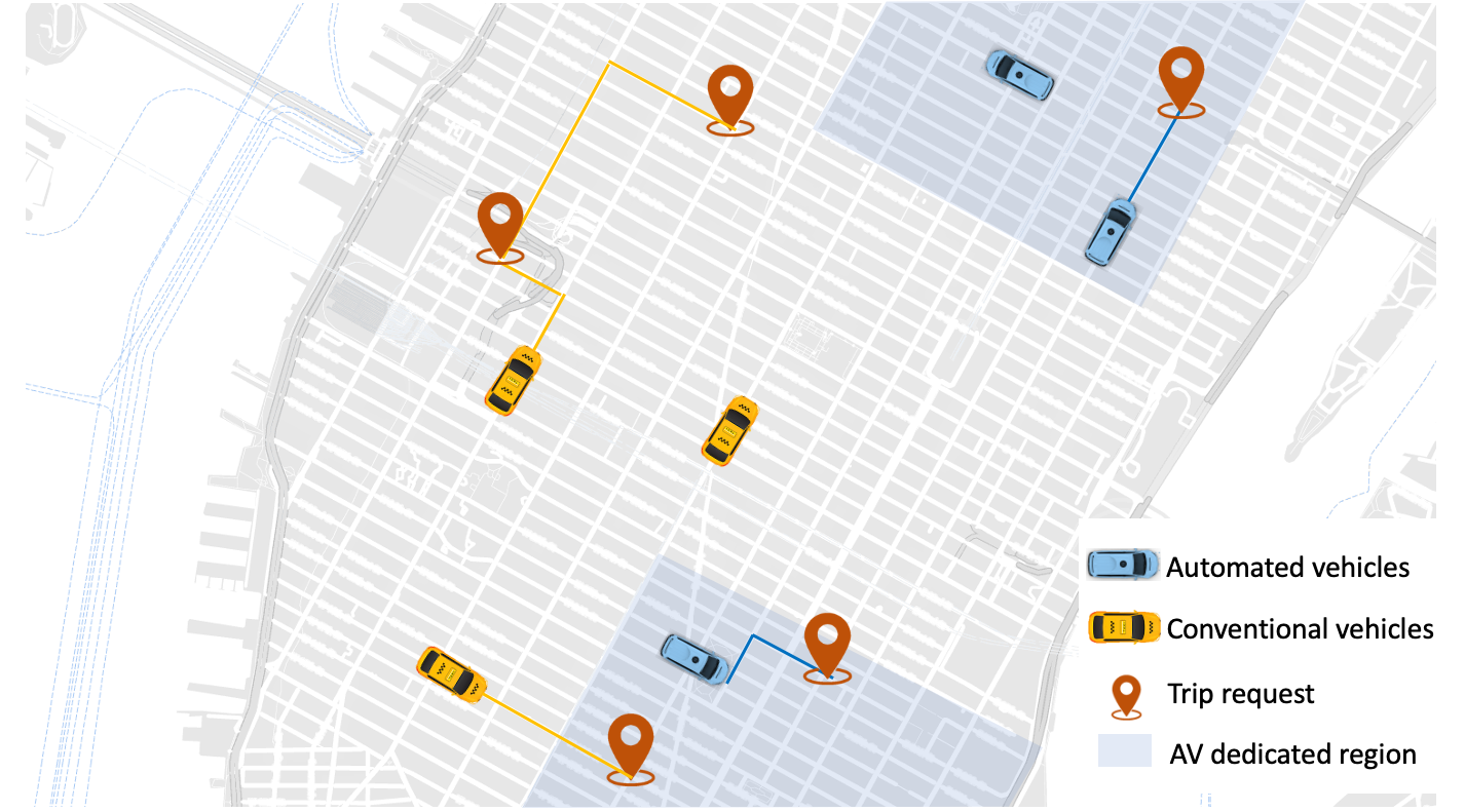
Figure 1: Example of ride-pooling with AVs and CVs. The first-stage decision is positioning vehicles in dedicated regions; The second-stage decisions are solving the assignment problem.

These examples address the importance of investigating the mixed-fleet operations problems. The platform’s decision in SRAMF is twofold: determining each supply source’s fleet size and location, which is termed the vehicle selection decision, and identifying potential ride-pooling assignments. The introduction of mixed fleets creates an endogenous source of stochasticity. The platform must make the vehicle selection decision before the actual demands are revealed (the detailed procedure is described in Figure 2).

It is critical to quantify how these sources of uncertainty affect the efficacy of ride-pooling assignment. For example, the platform with mixed autonomy fleets can only direct AVs to specific regions with roadside units or other road infrastructure (Chen et al. 2017b). If the number of AVs in each region does not match the estimated demand in the first stage, vehicle repositioning in the second stage is time-consuming and detrimental to the platform’s profitability.

1.2 Main Results and Contribution

The study’s primary objectives are to explain why solving the SRAMF problem is computationally intractable and to develop approximation algorithms for different vehicle fleets.

1. We prove that that SRAMF is NP-hard with any finite number of scenarios. Moreover, its objective does not have favorable submodular properties, which necessitates the development of new approximation algorithms.

2. Let $p$ denote the largest vehicular capacity plus one. For mid-capacity vehicles, we develop a local-search-based approximation algorithm with approximation ratio of $\frac{1}{p^{2}}$.

3. For high-capacity vehicles, we develop a primal-dual approximation algorithm with approximation ratio of $\frac{e-1}{(2e+o(1))p\ln p}$.

These polynomial-time algorithms leverage the special structure of shareability graphs to reduce the iteration load of evaluating different positioning policies in the first stage. Mid-capacity vehicles can carry less or equal to four requests, suitable for applications in Example 1 and Example 2. High-capacity vehicles can carry more than four requests, suitable for on-demand shuttles in Example 3. These approximation ratios are close to the best possible: no polynomial-time algorithm can achieve a ratio better than $O(\frac{\ln p}{p})$, under standard complexity assumptions.

This work focuses on the profit-maximization setting not only because of the practical concerns (Ashlagi et al. 2018, Simonetto, Monteil, and Gambella 2019) but also because developing approximation algorithms for maximizing GAPs is generally a more challenging task than minimizing GAPs (Fleischer et al. 2006). This study contributes to the growing literature on the operations of ridesharing and other mobility-on-demand platforms as follows:

1. Design algorithms with worst-case performance guarantees.  This work develops approximation algorithms to facilitate ride-pooling with mixed fleets with provable bounds in the stochastic setting. These algorithms are easy-to-implement and resemble the best possible bounds for GAP.

2. Evaluate the marginal value of increase fleet size in matching.  SRAMF necessitates the algorithm to assess the marginal value of including additional vehicles in the existing fleet. This proof technique is of independent interest to the broader fleet sizing studies (Benjaafar et al. 2021).

3. Demonstrate algorithms’ performance in a mixed-autonomy case study.  We demonstrate these algorithms’ computational efficiency and optimality gaps in a mixed autonomy traffic case study. The performance of these algorithms is competitive in real-data numerical experiments, and the derived worst-case approximation ratios are conservative.

This work focuses on the rolling-horizon approach with look-ahead demand estimates. Note that the exact method (i.e., MIP-based algorithms) in Alonso-Mora et al. (2017) and Ke et al. (2021) can also be replaced with these approximation algorithms to accelerate vehicle dispatching processes. The performance guarantee of any approximation algorithm built for the dual-source setting also holds for the single-source (Mori and Samaranayake 2021) and can be extended to mixed fleets of more than two vehicle types.

1.3 Organization and General Notation

The remainder of the paper is organized as follows. We first review the related literature in Section 2. Section 3 formulates the SRAMF problem and shows its hardness. Two approximation algorithms are proposed in Section 4 with nearly-tight approximation ratios. We test the effectiveness of these approximation algorithms using real-world and simulated data in Section 5 and draw conclusions in Section 6.

The following notation conventions are followed throughout this work. The notation $:=$ stands for “defined as”. For any integer $n$, we let $[n]:=\{1,2,\dots,n\}$. We use $v(\cdot)$ as the real value function and $\hat{v}(\cdot)$ as the approximate or estimated value function. P stands for the class of questions for which some algorithm can provide an answer in polynomial time, and NP stands for those with nondeterministic polynomial time algorithms. For any set $S$, $|S|$ is its cardinality, i.e., the number of elements in the set. Given two sets $A$ and $B$, we let $A+B$ or $A\cup B$ represent the union of $A$ and $B$; we let $A-B$ or $A\backslash B$ represent modifying $A$ by removing the elements belonging to $B$. We let $A\sim B$ denote that set $A$ intersects with $B$, i.e., $A\cap B\neq\varnothing$. i.i.d. stands for “independent and identically distributed”; w.r.t. stands for “with respect to”. Other notation and acronyms used in this paper are summarized in Table LABEL:table1 in Appendix 7.

2 Literature Review

We refer to ride-pooling (also called ride-splitting/carsharing rides) in the broad context and focus on operations-level decisions. The following review covers the recent development of computational methods for ride-pooling applications with different objectives of maximizing the utilization of vehicles or reducing the negative externalities related to deadhead miles.

Overview of ride-pooling algorithms.  Solving the optimal ride-pooling assignment is challenging in essence because a) the number of possible shared trips grows exponentially regarding the number of trip requests and the vehicle capacity; b) trip requests can be inserted during the trip. As a result, the exact approaches for solving the dynamic vehicle routing problem (DVRP) (Pillac et al. 2013) are not suitable for platforms that operates thousands of vehicles and expect to compute the assignment solutions in real-time.

Compared to the substantial body of literature for matching supply and demand without the ride-pooling option (Wang and Yang 2019), there exist only several attempts to solve the ride-pooling assignment problem by heuristic or decomposition methods (Yu and Shen 2019, Herminghaus 2019, Sundt et al. 2021). Although these methods achieved satisfying performance metrics in experiments, they cannot balance computational efficiency and accuracy with theoretical guarantees. This problem is tractable with fixed travel patterns such as providing services for daily commuting. Hasan, Van Hentenryck, and Legrain (2020) proposed a commute trip-sharing algorithm that maximized total shared rides for a set of commute trips satisfying various time-window, capacity, pairing, ride duration, and driver constraints.

Since the supply and demand processes are determined by previous decisions, the design of non-myopic policies that considers the future effects of assignments is attractive to platforms. Shah, Lowalekar, and Varakantham (2020) developed an approximate dynamic programming method that can learn from the IP-based assignment and approximate the value function by neural networks. Qin, Zhu, and Ye (2021) provided a comprehensive review of the current practice of reinforcement learning methods for assignment and other sequential decision-making problems in the ridesharing industry.

Scalable ride-pooling assignment algorithms for shareability graphs.  To tackle those unprecedented technical challenges in shared mobility platforms, Santi et al. (2014) quantified the trade-off between social benefits and passenger discomfort from ride-pooling by introducing the concept of “shareability networks”. They found that the total empty-car travel time was reduced 40% in the offline setting (i.e., with ex post demand profiles) or 32% when demands are revealed en route. This work suffers a limitation in capacity as the matching-based algorithm can only handle up to three-passenger shared rides.

Alonso-Mora et al. (2017) expanded the framework to up to ten riders per vehicle. The high-capacity ride-pooling trip assignment is solved by decomposing the shareability graph into trip sets and vehicle sets and then solving the optimal assignments by a large-scale integer program (IP). As the vehicle capacities increase, the moderate size of shared vehicle fleet ($2,000$ vehicles with capacities of four rides in their case studies) can serve most travel demand with short waiting time and trip delay. Simonetto, Monteil, and Gambella (2019) improved this approach’s computational efficiency by formulating the master problem as a linear assignment problem. The resulting large-scale assignment on shareability networks is calculated in a distributed manner. However, despite the easy implementation of these methods, they lack theoretical performance guarantees.

Approximation algorithms for maximization GAP.  Approximation algorithms can find near-optimal assignments with provable guarantees on the quality of returned solutions. Since the ride-pooling assignment problem is a variant of GAP (Öncan 2007), we list the significant results here. Shmoys and Tardos (1993) and Chekuri and Khanna (2005) transferred GAP to a scheduling problem and obtained polynomial-time $\frac{1}{2}$-approximation algorithms. Fleischer et al. (2006) obtained an LP-rounding based $(1-\frac{1}{e})$-approximation algorithm and a local-search based $\frac{1}{2}$-approximation algorithm.

Previous studies have explored GAP algorithms for both instant dispatching and batched dispatching settings. Instant dispatching assigns requests to available vehicles upon arrival. Lowalekar, Varakantham, and Jaillet (2020) developed approximation algorithms for online vehicle dispatch systems. Their setting with i.i.d. demand assumptions is markedly different from the current work. Batched dispatching utilizes GAP on a hypergraph to search for locally optimal assignments. Mori and Samaranayake (2021) developed $\frac{1}{e}$-approximation LP-rounding algorithms for the deterministic request-trip-vehicle assignment problem. In contrast, the current work considers two-stage decisions of fleet sizing and trip assignment with stochastic demand in SRAMF. As a batched dispatching algorithm, this stochastic formulation can be applied to arbitrary demand distributions.

Shared mobility with mixed fleets.  Mixed-fleet mobility systems are emerging research topics in the ridesharing literature. The first stream of researches is motivated by the change of workforce structure at present. Dong and Ibrahim (2020) investigated the staffing problem in ride-hailing platforms with a blended workforce of permanent employees and freelance workers. The platform needs to determine the number of hired drivers considering its impact on disclosing a flexible workforce. Dong et al. (2021) justified the dual-source strategy for mitigating the demand uncertainty in ride-hailing systems and designed optimal contracts to coordinate the mixed workforce. Castro et al. (2020) modeled the ridesharing market as matching queues where strategic drivers had different flexibility levels. They proposed a throughput-maximizing capacity reservation policy that is robust against drivers’ strategies.

The transition from traditional ridesharing services to AVs in the foreseeable future motivates a second stream of mixed-fleet researches. Lokhandwala and Cai (2018) used an agent-based model to evaluate the impact of heterogeneous preferences and revealed that the transition to a mixed fleet would reduce the total number of vehicles, focus on areas of dense demands, and lower the overall service levels in the suburban regions. Wei, Pedarsani, and Coogan (2020) studied the equilibrium of mixed autonomy network in which AVs are fully controlled by the platform and CVs are operated by individual drivers. The optimal pricing for the mixed service is formulated as a convex program. Lazar, Coogan, and Pedarsani (2020) proposed a network model for mixed autonomous traffic and showed how the price of anarchy in routing games was affected. In contrast, this work is one of the first attempts to develop algorithms for the operations of mixed fleets.

3 Problem Description

3.1 Basic Setting

This section introduces the formulation of the SRAMF problem as a two-stage stochastic program and shows its NP-hardness. These technical challenges motivate the design of new approximation algorithms in the remainder of this work.

3.1.1 Preliminaries: construction of shareability graph.

ride-pooling assignment is conducted on the shareability graph, which is represented by a hypergraph $G=\{S,D,E\}$. Here, $S$ denotes the supply/vehicles and $D$ denotes the demand/ride-requests; $S\cup D$ represents the vertices of the hypergraph. Each hyperedge $e\in E$ consists of one vehicle and a subset of ride-requests. In contrast to conventional ridesharing where each vehicle can only serve one ride-request per time (which corresponds to assignment on a bipartite graph), we consider the hypergraph generalization, where each hyperedge $e\in E$ can contain any number of ride-requests (within the vehicle’s capacity). Other constraints such as detour times and preferences for co-riders are also considered in the construction of the shareability graph (see Appendix 8). We also refer to hyperedges as cliques.

The mixed-fleet supply contains two separate sets of available vehicles $S_{A}$ and $S_{B}$ such that $S=S_{A}\cup S_{B}$, $|S_{A}|=n_{A}$, and $|S_{B}|=n_{B}$. The setup costs of vehicles in $S_{A}$ are significantly higher than those in $S_{B}$. We denote $p=1+\max_{i\in S_{A}\cup S_{B}}\{C_{i}\}$ where $C_{i}$ is the capacity of vehicle $i$. Without loss of generality, we let the cost of using vehicles in $S_{B}$ be $0$ and let the cost of each vehicle in $S_{A}$ be normalized to $1$. Depending on the specific applications, the setup cost can include the extra salary paid to full-time drivers (Example 1 and Example 2 in Section 1.1) or the cost of positioning AVs in advance (Example 3). The set $S_{B}$ is called the basis supply (which is always available) and the set $S_{A}$ is called the augmented supply (from which we need to select a limited number of vehicles). Section 4.3 discusses an extension to more than two vehicle types.

This setting is a generic model for shared mobility applications described in Section 1.1. Each hyperedge $e=\{i,J\}_{i\in S,J\subseteq D}$ corresponds to a potential trip where vehicle $i$ serves requests $J$. In the market segmentation example, the augmented supply includes available luxury-service vehicles. In the mixed autonomy traffic example, vacant CVs are the basis supply and potential locations to prearrange AVs are the augmented supply.

Solving the GAP problem on a hypergraph is the final step in the dispatching process (Alonso-Mora et al. 2017). The main analysis for SRAMF is conditional on having access to a hyperedge value oracle $\mathcal{O}(v_{e})$ that queries the expected profit obtained from any collection of requests in polynomial time. The hyperedge values $v_{e}$ include the total travel time of a Hamiltonian path $t$ picking up all requests $j\in e$. For completeness of deploying these proposed algorithms, Appendix 8 summarizes the preprocessing procedure.

3.1.2 Formulation of SRAMF.

Given a budget $K$, the platform chooses a subset $S_{R}\subset S_{A}$ of at most $K$ vehicles from the augmented supply. This decision is made before requests are revealed. After requests are revealed, the platform can only assign requests to these chosen vehicles $S_{R}\cup S_{B}$ and collect profits from finished trips immediately. Using a hypergraph representation, the second-stage assignment decision is equivalent to choosing a set of hyperedges in which every pair of hyperedges is disjoint. This condition guarantees that each vehicle and each request can be included no more than once in the final assignment.

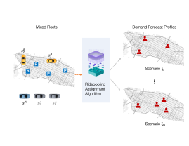
(a)

(b)

(c)

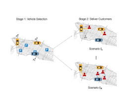
(d)

Figure 2: The illustration of SRAMF procedure per step. $S_{B}=\{s_{1}^{B},s_{2}^{B}\}$ is the basis set (e.g., CVs) and $S_{A}=\{s_{1}^{A},s_{2}^{A}\}$ is the augmented set (e.g., AVs). In the first step in Figure 2a, the algorithm observes the current locations of $S_{A}$ and $S_{B}$ and obtain demand forecast. In the second step in Figure 2b, the algorithm constructs the shareability graph for each scenario, where each trip is a clique containing one vehicle and multiple matchable requests. In the third step in Figure 2c, the SRAMF problem is solved by the approximation algorithm. In the final step in Figure 2d, the two-stage decisions are implemented and the system state is updated. In each scenario $\xi$, one or more requests are linked by the assigned vehicle in a single ride.

To be more specific in implementation, the sequence of decision-making in SRAMF is as follows:

1. For each vehicle $i\in S_{A}$, we let $y_{i}=1$ denote if we put the vehicle in service and $y_{i}=0$ if not. These augmented vehicles or potential locations to preposition vehicles are spatially distant from each other and behave differently in the assignment stage. We use $S_{R}:=\{i\in[n_{A}]:y_{i}=1\}\subseteq S_{A}$ to denote all selected augmented vehicles. All vehicles in the basis supply are included in the first-stage decision as they are no cost to use; i.e., we set $y_{i}=1$ for all $i\in S_{B}$. So, the chosen supply is $S_{R}\cup S_{B}$. The first-stage decision space is $Y\in\{0,1\}^{n_{A}+n_{B}}$.

2. In the second-stage, the platform observes the realized scenario $\xi$, which corresponds to a set of ride-requests $D(\xi)$ and hyperedges $E(\xi)$; we also observe the values of all hyperedges. The scenario $\xi$ follows a random distribution $F(\xi)$ with support on $\Xi$, which is incorporated into a demand forecast model.

   Each hyperedge $e\in E(\xi)$ includes some vehicle $i$ and a subset of requests $J\subset D(\xi)$. The total number of passengers in the ride-requests $J$ must be at most the capacity $C_{i}$ of vehicle $i$, i.e., $\sum_{j\in J}w_{j}\leq C_{i}$ where $\{w_{j}\}_{j\in J}$ denote the numbers of passengers in each ride-request. The hyperedge’s value considers following elements:

   1. The expected profit $u_{j}$ gained from serving the request $j$.

   2. Trip $t=\{j_{1},j_{2},\dots:j_{k}\in J\}$ as a sequence of requests and the associated traveling cost $c(i,t)$ for vehicle $i$ to pick up all requests.

   3. Each request $j$ gains additional utility $\tilde{u}_{ij}$ if matched with their preferred vehicle type.

   The hyperedge value for $e\in E(\xi)$ collected from a potential assignment is given by

   $$v_{e}=\sum_{j\in J}u_{j}+\sum_{j\in J}\tilde{u}_{ij}-c(i,t)\geq 0.$$ (1)

   This value captures many stochastic factors at play between the 1st and 2nd stages, i.e., vehicle selection and trip assignment. $u_{j}$ considers the uncertain number of trip requests and their origin and destination; $w_{j}$ and the set $J$ considers the unknown number of passengers in each trip request; $\tilde{u}_{ij}$ considers the customers’ uncertain preference for vehicle types. Finally, due to fluctuating traffic conditions and different vehicle technology (e.g., CVs and AVs), $c(i,t)$ represents that pickup times are uncertain. However, in the 2nd stage (after the scenario $\xi$ is observed), all hyperedge values are known precisely.

   In addition, the batched dispatch can be expanded to more general policies by using more advanced value function approximation. For example, Tang et al. (2019) calculated the associated hyperedge value as a reward signal derived from a reinforcement-learning-based estimator.

3. The platform assigns ride-requests to each available vehicle by determining $x_{e}\in\{0,1\}$ for all $e\in E(\xi)$. The assignment is only available between the chosen supply $S_{R}\cup S_{B}$ (denoted as $e\sim S_{R}\cup S_{B}$) and realized demand $D(\xi)$ in each scenario.

The optimal value of assignments in scenario $\xi$ is denoted by $Q(y,\xi)$ supported on $Q:Y\times\Xi\to\mathbb{R}$. Given a scenario, the second-stage decisions are trip assignments denoted by $x=\{x_{e}\}_{e\in E(\xi)}$. Our objective is to maximize the expected total value.

The SRAMF problem can be formulated as a two-stage stochastic program:

$$\operatorname*{maximize}_{y}\mathbf{E}[Q(y,\xi)]$$ (2)

$$s.t. \sum_{i\in S_{A}}y_{i}\leq K$$ (budget) (2a)

$$y_{i}\in\{0,1\} \forall i\in S_{A}\cup S_{B},$$ (2b)

and the second-stage problem is given by

$$Q(y,\xi) =\operatorname*{maximize}_{x}\sum_{e\in E(\xi)}v_{e}x_{e}$$ (3)

$$s.t. \sum_{e\in E(\xi):j\in e}x_{e}\leq 1 \forall j\in D(\xi)\quad\textit{(assignment I ) }$$ (3a)

$${\color[rgb]{0,0,0}\sum_{e\in E(\xi):i\in e}x_{e}\leq y_{i}} {\color[rgb]{0,0,0}\forall i\in S_{B}\cup S_{A}\quad\textit{(assignment II )}}$$ (3b)

$$x_{e}\in\{0,1\} \forall e\in E(\xi).$$ (3c)

In the first-stage problem (2), $K$ is the maximum number of chosen vehicles from the augmented supply. In the second-stage problem (3), the constraints (3a) and (3b) guarantee that each supply and demand are matched at most once and only the vehicles selected in the first stage are used. We allow both vehicles and requests to remain unassigned in the hypermatching $x$. The second-stage problem is also known as the $p$-set packing problem, where ($p-1$) denotes the maximum number of requests per hyperedge (e.g.,  Füredi, Kahn, and Seymour (1993) and Chan and Lau (2012)). This $p$-set packing problem is already NP-hard.

3.1.3 Road-map for proving SRAMF approximation algorithms.

Figure 3 provides an overview of the performance analysis on two proposed approximation algorithms and their approximation ratios, respectively. We start with reducing the objective of (2) to the sample-average estimate in Section 3.2. We then show the hardness of the SRAMF problem in Section 3.3. A key challenge is that the 2nd stage problem (3) is itself NP-hard. So, our approximation algorithms rely heavily on “fractional assignments” that relax the integrality constraints in (3) and can be solved in polynomial-time via linear programming. We provide two different approximations algorithms, LSLPR and MMO, in Section 4.1 and Section 4.2, respectively.

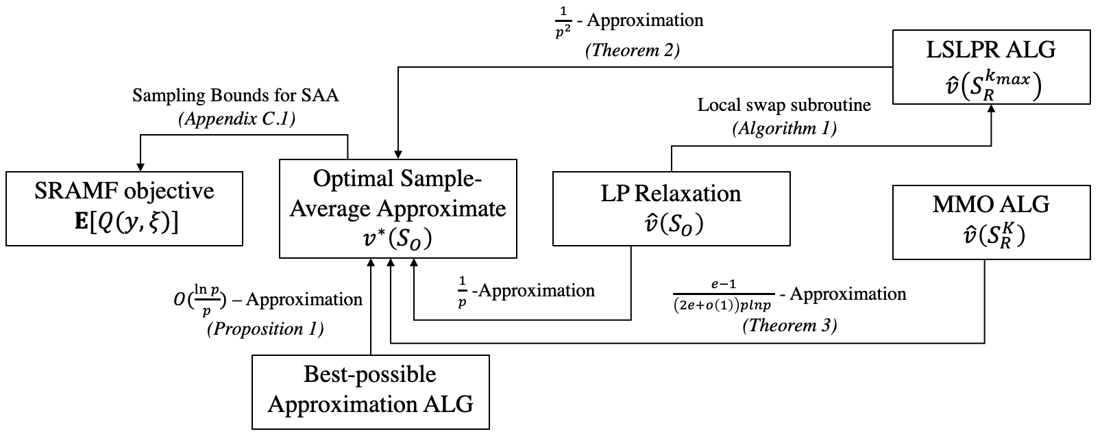
Figure 3: An illustration of the performance analysis on SRAMF algorithms; the approximation ratios on arrows refer to the results in this paper; $S_{O}$ is the optimal selection of vehicles and $S_{R}$ is the section of vehicles generated by approximation algorithms.

3.2 Reduction to Sample-Average Estimate

The sample-average approximation (SAA) method is commonly used to solve such two-stage stochastic programs. It draws $N$ scenarios $\{\xi_{\ell}\}_{\ell=1}^{N}$ from a scenario-generating oracle (e.g., demand forecasting and vehicle simulation models) and approximates the expected objective function by a sample-average estimate $\mathbf{E}[Q(y,\xi)]\approx\frac{1}{N}\sum_{\ell=1}^{N}Q(y,\xi_{\ell})$.

To simplify the analysis with regard to $\mathbf{E}(Q(y,\xi))$, we reduce the objective function to finite-sample proximity. The main analysis is conditional on $N$ mutually disjoint sets of hyperedges as $E(\xi)$. Since the second-stage assignment ensures unique matching per scenario, we can make $n^{\prime}$ copies when a trip consisting of one vehicle and several requests duplicates across $n^{\prime}$ scenarios. The consistency and shrinking bias of the sample-average estimate are well-studied in literature. The optimal value of any approximation algorithm converges to $\mathbf{E}[Q(y,\xi)]$ as the number of scenarios $N\to\infty$. We include the standard SAA proof in Appendix 7 for completeness of the results, which helps determine the required sample size $N$ for any confidence level.

The current paper’s focus is developing algorithms to solve the SRAMF problem in eq.(2) with the sample-average estimate. As mentioned earlier, we will work with an LP relaxation of (3) as the original problem is NP-hard. For any subset $S_{R}\subseteq S_{A}$ and scenario $\xi$, define $\hat{v}(S_{R},\xi)$ to be the optimal value of the following LP:

$$\operatorname*{maximize}_{x} \sum_{e\in E(\xi)}v_{e}x_{e}$$ (4)

$$s.t. \sum_{e\in E(\xi):j\in e}x_{e}\leq 1 \forall j\in D(\xi)$$ (4a)

$$\sum_{e\in E(\xi):i\in e}x_{e}\leq 1 \forall i\in S_{A}\cup S_{B}$$ (4b)

$$x_{e}=0 \forall e\sim S_{A}\setminus S_{R}$$ (4c)

$$x_{e}\geq 0 \forall e\in E(\xi).$$ (4d)

We call the LP solution “fractional assignments”. Also, define ${v}(S_{R},\xi)$ to be the optimal value of the IP corresponding to the formulation above; so ${v}(S_{R},\xi)$ equals the optimal value in (3). These are used to define two useful objective functions w.r.t. $S_{R}$:

• The objective value using the exact GAP in eq.(3) for each scenario is given by:

  $$v^{*}(S_{R})=\frac{1}{N}\sum_{\ell\in[N]}v(S_{R},\xi_{\ell}).$$ (5)

• The objective value using the LP-relaxation (4) is given by:

  $$\hat{v}(S_{R})=\frac{1}{N}\sum_{\ell\in[N]}\hat{v}(S_{R},\xi_{\ell}).$$ (6)

Fractional assignments enjoy many well-known properties. First, the integrality gap of the above LP relaxation for $p$-set packing is at most $p$  (Arkin and Hassin 1998). Second, a greedy algorithm that selects hyperedges $e$ in decreasing order of their values $v_{e}$ (while maintaining feasibility) also achieves a $\frac{1}{p}$-approximation to the LP value. We restate them in the following theorem:

Theorem 3.1

For any $S_{R}\subseteq S_{A}$, we have $v^{*}(S_{R})\leq\hat{v}(S_{R})\leq p\cdot v^{*}(S_{R})$; furthermore, the greedy algorithm obtains a solution of value at least $\frac{1}{p}\cdot\hat{v}(S_{R})$.

These reductions narrow down the main task to bounding the approximation ratios with regard to $\hat{v}(S_{R})$. In particular, we will focus on the SRAMF problem with fractional assignments:

$$\max_{S_{R}\subseteq S_{A}:|S_{R}|\leq K}\quad\hat{v}(S_{R}).$$ (7)

If we obtain an $\alpha$-approximation algorithm for (7), then combined with Theorem 3.1, we would obtain an $\frac{\alpha}{p}$-approximation algorithm for SRAMF (with integral assignments).

Before jumping into the design of approximation algorithms, the following subsection elaborates on some technical challenges.

3.3 Hardness and Properties of SRAMF

We show that solving SRAMF is computationally challenging due to the following reasons. First, the second-stage SRAMF problem is NP-hard in general, as demonstrated in Proposition 3.2. Second, Proposition 3.4 shows that $\hat{v}(S_{R})$ is not submodular, which prevents the use of classic algorithms such as (Nemhauser, Wolsey, and Fisher (1978)). These facts motivate the development of new approximation algorithms in Section 4.

Proposition 3.2

There is no algorithm for SRAMF (even with $N=1$ scenario) with an approximation ratio better than $O(\frac{\ln p}{p})$, unless $P=NP$.

Proof 3.3

Proof for the hardness of SRAMF : We reduce from the $p$-dimensional matching problem, defined as follows. There is a hypergraph $H$ with vertices $V$ partitioned into $p$ parts $\{V_{r}\}_{r=1}^{p}$, and hyperedges $E$. Each hyperedge contains exactly one vertex from each part (so each hyperedge has size exactly $p$). The goal is to find a collection $F$ of disjoint hyperedges that has maximum cardinality $|F|$.

Given any instance of $p$-dimensional matching (as above), we generate the following SRAMF instance. The augmented vehicles are $S_{A}=V_{1}$ and the basis vehicles are $S_{B}=\varnothing$. There is $N=1$ scenario with ride-requests $V_{2}\cup\dots V_{p}$ and hyperedges $E$ (each of value $1$). Each vehicle has capacity $p-1$ and each ride-request has $1$ passenger. Note that each hyperedge contains exactly one vehicle, as required in SRAMF. The bound $K=|S_{A}|$: so the optimal 1st stage solution is clearly $S_{R}=S_{A}$ (select all augmented vehicles). Now, the SRAMF problem instance reduces to its 2nd stage problem (3), which involves selecting a maximum cardinality subset of disjoint hyperedges. This is precisely the $p$-dimensional matching problem.

It follows that if there is any $\alpha$-approximation algorithm for SRAMF with $N=1$ scenario then there is an $\alpha$-approximation algorithm for $p$-dimensional matching. Finally, Hazan, Safra, and Schwartz (2006) proved that it is NP-hard to approximate $p$-dimensional matching better than an $O(\frac{\ln p}{p})$ factor (unless $P=NP$). The proposition now follows. $\square$

This intractability is the reason that we work with the fractional assignment problem (7). A natural approach for budgeted maximization problems such as (7) is to prove that the objective function is submodular, in which case one can directly use the $(1-\frac{1}{e})$-approximation algorithm by (Nemhauser, Wolsey, and Fisher 1978). However, we show a negative result about the submodularity of $v^{*}(S_{R})$ as well as $\hat{v}(S_{R})$, which precludes the use of such an approach. Recall that a set function $f:2^{\Omega}\rightarrow\mathbb{R}_{+}$ on groundset $\Omega$ is submodular if $f(U\cup\{i\})-f(U)\geq f(W\cup\{i\})-f(W)$ for all $U\subseteq W\subseteq\Omega$ and $i\in\Omega\setminus W$.

Proposition 3.4

$v^{*}(S_{R})$ and $\hat{v}(S_{R})$ are not submodular functions.

Proof 3.5

Proof: Recall that the groundset for both functions $v^{*}$ and $\hat{v}$ is $\Omega:=S_{A}$ the set of augmented vehicles. We provide an SRAMF instance with $N=1$ scenario where these functions are not submodular. Consider a shareability graph with $|S_{A}|=3$, $S_{B}=\varnothing$ and three ride-requests $\{d_{1},d_{2},d_{3}\}$. Let $p=3$, i.e., each vehicle can carry at most two requests. The set of hyperedges is

$$\{(s_{1}^{A},d_{1}),(s_{1}^{A},d_{2},d_{3}),(s_{2}^{A},d_{2}),(s_{3}^{A},d_{3})\}.$$

See also Figure 4. The value of each hyperedge is the number of ride-requests covered by it.

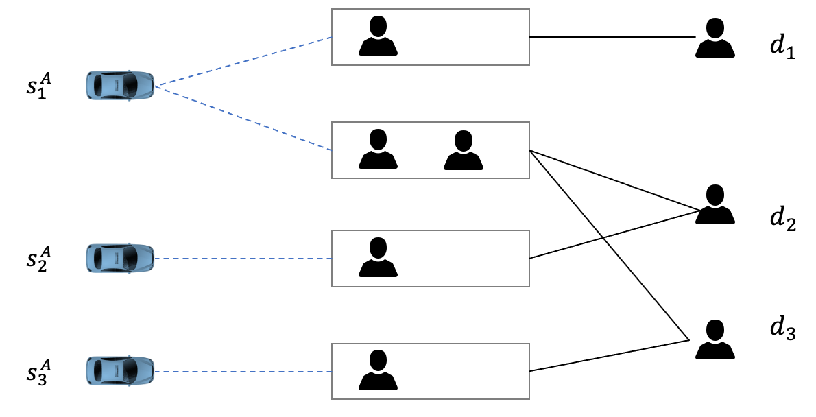
Figure 4: An example for non-submodularity of function $v^{*}(S_{R})$.

Let subsets $U=\{s_{1}^{A}\}$ and $W=\{s_{1}^{A},s_{2}^{A}\}$. Also let $i=s_{3}^{A}$. Clearly, $v^{*}(U)=2$ (serving $d_{2},d_{3}$), $v^{*}(W)=2$ (serving $d_{1},d_{2}$ or $d_{2},d_{3}$), $v^{*}(U\cup\{i\})=2$ (serving $d_{1},d_{3}$ or $d_{2},d_{3}$), and $v^{*}(W\cup\{i\})=3$. Therefore, we have:

$$v^{*}(W\cup\{i\})-v^{*}(W)=1>0=v^{*}(U\cup\{i\})-v^{*}(U),$$

which implies the set function $v^{*}$ is not submodular. It is easy to check that the LP value function $\hat{v}=v^{*}$ for this instance: so function $\hat{v}$ is also not submodular. $\square$

4 Approximation Algorithms for SRAMF

This section provides two different approximation algorithms for SRAMF. Both the algorithms focus on solving the fractional assignment problem (7), and achieve approximation ratios $\frac{1}{p}$ and $\approx\frac{e-1}{2e\cdot\ln p}$ respectively. Combined with Theorem 3.1, these imply approximation algorithms for SRAMF with an additional factor of $\frac{1}{p}$.

4.1 Local Search Algorithm for Mid-Capacity SRAMF

The Mid-Capacity SRAMF models the current ride-hailing market where the limit for palletizing requests is two or three. In this section, we propose a Local-Search LP-Relaxation (LSLPR) algorithm that obtains $\frac{1}{p}$-approximation for the fractional problem (7).

4.1.1 Overview of the LSLPR algorithm.

Let $\epsilon>0$ be an arbitrarily small parameter that will be used in the stopping criterion. The outline of the LSLPR algorithm is as follows:

1. Start from any solution $S_{R}\subseteq S_{A}$ with $|S_{R}|=K$.

2. Consider all solutions $S_{R^{\prime}}=S_{R}-\{i\}+\{i^{\prime}\}$ where $i\in S_{R}$ and $i^{\prime}\notin S_{R}$ (i.e., swapping one vehicle) and evaluate the corresponding LP value $\hat{v}(S_{R^{\prime}})$.

3. Change the current solution $S_{R}$ to $S_{R^{\prime}}$ if the objective value improves significantly, i.e., $\hat{v}(S_{R^{\prime}})>(1+\epsilon)\cdot\hat{v}(S_{R})$.

4. Stop when the current solution does not change.

Formally, let $k$ index the iterations, where the current solution changes in each iteration. Let $S_{R}^{k}$ denote the current solution at the start of iteration $k$. The following subroutine implements a single iteration.

for $i\in S_{R}^{k}$ and $i^{\prime}\in S_{A}\backslash S_{R}^{k}$ do

       obtain $\hat{v}(S^{k}_{R}-i+i^{\prime})$ by solving an LP ;

      

end for

let $(c,c^{\prime})$ be the pair that maximizes $\hat{v}(S^{k}_{R}-i+i^{\prime})$ over $i\in S_{R}^{k}$ and $i^{\prime}\in S_{A}\backslash S_{R}^{k}$;

if $\hat{v}^{*}(S^{k}_{R}-c+c^{\prime})>(1+\epsilon)\cdot\hat{v}(S^{k}_{R})$ then

       set $S_{R}^{k+1}\leftarrow S^{k}_{R}-c+c^{\prime}$ and continue with $k\leftarrow k+1$ ;

      

else

      halt local search and output $S^{k}_{R}$;

      

end if

Algorithm 1 Local swap subroutine.

In a broad sense, the local swap subroutine does not necessarily enumerate all pairs $(i,i^{\prime})$ to search for the optimal $(c,c^{\prime})$. A more efficient alternative is terminating each iteration at the first pair of $i\in S_{R}$ and $i^{\prime}\in S_{A}\backslash S_{R}$ that increases the objective by more than $\epsilon\cdot\hat{v}(S_{R}^{k})$. The complete LSLPR algorithm is now as follows:

Data: Augmented supply $S_{A}$, basis supply $S_{B}$, scenarios $\{\xi_{\ell}\}_{\ell=1}^{N}$ and $\epsilon>0$.

Result: Near-optimal $S_{R}\subset S_{A}$ and the corresponding trip assignment.

Initialization: Set $k=1$ and randomly select $K$ vehicles from $S_{A}$ as $S^{1}_{R}$;

while $k\leq k_{\max}$ do

      Run the local swap subroutine in Algorithm 1;

      

end while

Obtain the final trip assignment with $S_{R}=S^{k_{\max}}_{R}$ using the greedy algorithm (Theorem 3.1).

Algorithm 2 Local search LP-relaxation algorithm for SRAMF

Algorithm 2 obtains the final selection of vehicles $S^{k_{\max}}_{R}$ where the maximal number of iterations will be derived below. In the final step, the algorithm obtains an integral assignment for each scenario instead of the fractional assignments in $\hat{v}(S_{R})$. To this end, we use the greedy algorithm (Theorem 3.1) to select the assignment for each scenario, which is guaranteed to have value at least $\frac{1}{p}$ times the fractional assignment. In Section 4.1.2, we first analyze the approximation ratio and then the computational complexity of LSLPR.

4.1.2 Analysis of the LSLPR algorithm.

Recall that $S_{R}$ is the locally optimal solution obtained by our algorithm. Let $S_{O}$ denote the optimal solution; note that $S_{O}$ is a fixed subset that is only used in the analysis. Also, let $\boldsymbol{x}=\langle\boldsymbol{x}^{\xi}\rangle$ and $\boldsymbol{z}=\langle\boldsymbol{z}^{\xi}\rangle$ denote the optimal LP solutions to $\hat{v}(S_{R})$ and $\hat{v}(S_{O})$, respectively.

It will be convenient to consider the overall hypergraph on vertices $S_{A}\cup S_{B}\cup\left(\cup_{\xi}D(\xi)\right)$ and hyperedges $\cup_{\xi}E(\xi)$. By duplicating hyperedges (if necessary), we may assume that $E(\xi)$ are disjoint across scenarios $\xi$. Recall that $\boldsymbol{x}^{\xi}$ (and $\boldsymbol{z}^{\xi}$) has a decision variable corresponding to each hyperedge in $E(\xi)$. For each demand $d\in\cup_{\xi}D(\xi)$, let $H_{d}$ denote the hyperedges incident to it. For each vehicle $i\in S_{A}\cup S_{B}$ and scenario $\xi$, let $E_{i,\xi}$ denote the hyperedges in $E(\xi)$ containing $i$. So, $F_{i}:=\cup_{\xi}E_{i,\xi}$ is the set of hyperedges incident to vehicle $i$.

For any demand $d$, the following lemma sets up a mapping between the hyperedges (incident to $d$) used in the solutions $\boldsymbol{x}$ and $\boldsymbol{z}$. For the analysis, we add a dummy hyperedge $\bot$ incident to $d$ so that the assignment constraints in the LP solutions $\boldsymbol{x}$ and $\boldsymbol{z}$ are binding at $d$. So, $\sum_{e\in H_{d}}x_{e}+x_{\bot}=1$ and $\sum_{f\in H_{d}}z_{f}+z_{\bot}=1$. Let $H^{\prime}_{d}:=H_{d}\cup\{\bot\}$ denote the hyperedges incident to $d$.

Lemma 4.1

For any demand $d$, there exists a decomposition mapping $\Delta_{d}:H^{\prime}_{d}\times H^{\prime}_{d}\to\mathbb{R}$ satisfying the following conditions:

1. $\Delta_{d}(e,f)\geq 0$ for all $e,f\in H_{d}^{\prime}$;

2. $\sum_{e\in H^{\prime}_{d}}\Delta_{d}(e,f)=z_{f}$ for all $f\in H^{\prime}_{d}$;

3. $\sum_{f\in H^{\prime}_{d}}\Delta_{d}(e,f)=x_{e}$ for all $e\in H^{\prime}_{d}$.

Figure 5 illustrates this mapping. Appendix 9 includes the definition of $\Delta_{d}(e,f)$ and the proof for Lemma 4.1. Note that $\sum_{e\in H^{\prime}_{d}}\sum_{f\in H^{\prime}_{d}}\Delta_{d}(e,f)=1$ for any demand $d$. For any subset $F\in H_{d}^{\prime}$, we use the shorthand $\Delta_{d}(e,F):=\sum_{f\in F}\Delta_{d}(e,f)$.

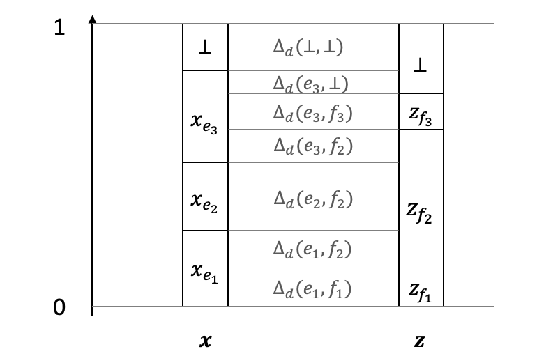
Figure 5: Illustration of mapping $\Delta_{d}(e,f)$.

Here is an outline of the remaining analysis. Let ${\cal L}$ denote any bijection between $S_{R}$ (algorithm’s solution) and $S_{O}$ (optimal solution), consisting of pairs $(i_{1},i_{2})$ where $i_{1}\in S_{R}$ and $i_{2}\in S_{O}$. We first consider a swap $S_{R}-i_{1}+i_{2}$ where $(i_{1},i_{2})\in{\cal L}$, and lower bound the objective increase. Note that the local optimality of $S_{R}$ implies that the objective increase is at most $\epsilon\cdot\hat{v}(S_{R})$. Then, we add the inequalities corresponding to the objective increase for the swaps in ${\cal L}$ and obtain the approximation ratio.

Analysis of a single swap $(i_{1},i_{2})$.  Consider any $i_{1}\in S_{R}$ and $i_{2}\in S_{O}$. We now lower bound $\hat{v}(S_{R}-\{i_{1}\}+\{i_{2}\})-\hat{v}(S_{R})$. Recall that for any subset $S$, $\hat{v}(S)=\frac{1}{N}\sum_{\xi}\hat{v}(S,\xi)$ where $\hat{v}(S,\xi)$ is the LP value for scenario $\xi$. So, we have

$$\hat{v}(S_{R}-\{i_{1}\}+\{i_{2}\})-\hat{v}(S_{R})=\frac{1}{N}\sum_{\xi}\left(\hat{v}(S_{R}-\{i_{1}\}+\{i_{2}\},\xi)-\hat{v}(S_{R},\xi)\right).$$

We now focus on a single scenario $\xi$ and lower bound $\hat{v}(S_{R}-\{i_{1}\}+\{i_{2}\},\xi)-\hat{v}(S_{R},\xi)$. To this end, we will define a feasible solution $\bar{\boldsymbol{x}}^{\xi}$ for the LP $\hat{v}(S_{R}-\{i_{1}\}+\{i_{2}\},\xi)$. Recall that $\boldsymbol{x}^{\xi}$ denotes the optimal solution for LP $\hat{v}(S_{R},\xi)$. So, we can then bound:

$$\hat{v}(S_{R}-\{i_{1}\}+\{i_{2}\},\xi)-\hat{v}(S_{R},\xi)\quad\geq\quad\boldsymbol{v}^{\intercal}\bar{\boldsymbol{x}}^{\xi}-\boldsymbol{v}^{\intercal}\boldsymbol{x}^{\xi},$$ (8)

where $\boldsymbol{v}$ is the vector of hyperedge values for $E(\xi)$. As we focus on a single scenario $\xi$, we drop $\xi$ from the notation whenever it is clear.

We are now ready to construct the new fractional assignment $\bar{\boldsymbol{x}}$. Define:

1. $\bar{x}_{e}=0$ for all $e\in F_{i_{1}}$. This corresponds to dropping vehicle $i_{1}$ from $S_{R}$.

2. $\bar{x}_{e}=z_{e}$ for all $e\in F_{i_{2}}$. This corresponds to adding vehicle $i_{2}$ to $S_{R}$.

3. $\bar{x}_{e}=x_{e}-\max_{d\in e}\Delta_{d}(e,F_{i_{2}}\cap H_{d})$ for all $e\in E(\xi)\setminus F_{i_{1}}\setminus F_{i_{2}}$.

If $i_{1}=i_{2}$ then we simply drop case 1 above. The third case above is needed to make space for the hyperedges incident to the new vehicle $i_{2}$ (which are increased in case 2). The following two lemmas prove the feasibility of this solution $\bar{\boldsymbol{x}}$ and bound its objective value. Below, we assume that $i_{1}\neq i_{2}$ (the proof for $i_{1}=i_{2}$ is nearly the same, in fact even simpler).

Lemma 4.2

$\bar{\boldsymbol{x}}$ is a feasible solution for $\hat{v}(S_{R}-\{i_{1}\}+\{i_{2}\})$.

Proof 4.3

Proof for Lemma 4.2:

We show the feasibility by checking all constraints in eq.(4). Note that $\bar{x}_{e}=0$ for all hyperedges $e$ incident to a vehicle in $S_{A}\setminus\left(S_{R}-\{i_{1}\}+\{i_{2}\}\right)$.

Constraint $\bar{\boldsymbol{x}}\geq 0$. It suffices to check this for hyperedges $e\in E\setminus F_{i_{1}}\setminus F_{i_{2}}$. Note that

$$\bar{x}_{e}=x_{e}-\max_{d\in e}\Delta_{d}(e,F_{i_{2}}\cap H_{d})=\min_{d\in e}\left(x_{e}-\Delta_{d}(e,F_{i_{2}}\cap H_{d})\right)\geq 0,$$

where the inequality uses Lemma 4.1, i.e., $x_{e}=\Delta_{d}(e,H^{\prime}_{d})\geq\Delta_{d}(e,F_{i_{2}}\cap H_{d})$.

Constraint (4a): By definition of $\bar{\boldsymbol{x}}$, for any demand $d$, we have:

$$\sum_{e\in H_{d}}\bar{x}_{e} =\sum_{e\in H_{d}\cap F_{i_{2}}}z_{e}+\sum_{e\in H_{d}\setminus F_{i_{1}}\setminus F_{i_{2}}}\left[x_{e}-\Delta_{d}(e,F_{i_{2}}\cap H_{d})\right]$$

$$\leq\sum_{e\in H_{d}\cap F_{i_{2}}}z_{e}+\sum_{e\in H^{\prime}_{d}}\left[x_{e}-\Delta_{d}(e,F_{i_{2}}\cap H_{d})\right]$$

$$=\sum_{e\in H_{d}\cap F_{i_{2}}}z_{e}+\sum_{e\in H^{\prime}_{d}}x_{e}-\sum_{f\in F_{i_{2}}\cap H_{d}}\Delta_{d}(H^{\prime}_{d},f)$$

$$=\sum_{e\in H^{\prime}_{d}}x_{e}\,\,=\,\,1.$$

Constraint (4b): The augmented vehicle set can be divided into three groups.

1. Vehicle $i_{1}$: $\sum_{e\in F_{i_{1}}}\bar{x}_{e}=0$.

2. Vehicle $i_{2}$: $\sum_{e\in F_{i_{2}}}\bar{x}_{e}=\sum_{e\in F_{i_{2}}}z_{e}\leq 1$ by definition.

3. Vehicles $j\neq i_{1},i_{2}$: $\sum_{e\in F_{j}}\bar{x}_{e}\leq\sum_{e\in F_{j}}x_{e}\leq 1$.

Therefore, $\bar{\boldsymbol{x}}$ is a feasible fractional assignment solution. $\square$

Lemma 4.4

The increase in objective is:

$$\sum_{e\in E(\xi)}v_{e}(\bar{x}^{\xi}_{e}-x^{\xi}_{e})\geq\sum_{e\in F_{i_{2}}\cap E(\xi)}v_{e}z^{\xi}_{e}-\sum_{f\in F_{i_{1}}\cap E(\xi)}v_{f}x^{\xi}_{f}-\sum_{e\in E(\xi)}v_{e}\sum_{d\in e}\Delta_{d}(e,F_{i_{2}}\cap H_{d}).$$

Proof 4.5

Proof for Lemma 4.4: By definition of $\bar{\boldsymbol{x}}$,

$$\bar{x}_{e}-x_{e}=\begin{cases}z_{e}&\text{ if }e\in F_{i_{2}}\\ -x_{e}&\text{ if }e\in F_{i_{1}}\\ -\max_{d\in e}\Delta_{d}(e,F_{i_{2}}\cap H_{d})&\text{ otherwise}\end{cases}.$$

Note that $x_{e}=0$ for all $e\sim S_{A}\backslash S_{R}$ in $\hat{v}(S_{R})$. So we have

$$\sum_{e\in E(\xi)}v_{e}(\bar{x}_{e}-x_{e}) \geq\sum_{e\in F_{i_{2}}\cap E(\xi)}v_{e}z_{e}-\sum_{f\in F_{i_{1}}\cap E(\xi)}v_{f}x_{f}-\sum_{e\in E(\xi)}v_{e}\max_{d\in e}\Delta_{d}(e,F_{i_{2}}\cap H_{d})$$

$$\geq\sum_{e\in F_{i_{2}}\cap E(\xi)}v_{e}z_{e}-\sum_{f\in F_{i_{1}}\cap E(\xi)}v_{f}x_{f}-\sum_{e\in E(\xi)}v_{e}\sum_{d\in e}\Delta_{d}(e,F_{i_{2}}\cap H_{d}).$$

$\square$

Combining Lemmas 4.2 and 4.4, and adding over all scenarios $\xi$, we obtain:

Lemma 4.6

For any $i_{1}\in S_{R}$ and $i_{2}\in S_{O}$, we have

$$\hat{v}(S_{R}-\{i_{1}\}+\{i_{2}\})-\hat{v}(S_{R})\geq\sum_{e\in F_{i_{2}}}v_{e}z_{e}-\sum_{f\in F_{i_{1}}}v_{f}x_{f}-\sum_{e\in E}v_{e}\sum_{d\in e}\Delta_{d}(e,F_{i_{2}}\cap H_{d}).$$

Combining all the swaps.  Recall that ${\cal L}$ is a bijection between $S_{R}$ and $S_{O}$. Using the local optimality of $S_{R}$,

$$K\epsilon\cdot\hat{v}(S_{R})\geq \sum_{(i_{1},i_{2})\in\mathcal{L}}\left[\hat{v}(S_{R}-\{i_{1}\}+\{i_{2}\})-\hat{v}(S_{R})\right]$$

$$\geq \sum_{(i_{1},i_{2})\in\mathcal{L}}\left[\sum_{e\in F_{i_{2}}}v_{e}z_{e}-\sum_{f\in F_{i_{1}}}v_{f}x_{f}-\sum_{e\in E}v_{e}\sum_{d\in e}\Delta_{d}(e,F_{i_{2}}\cap H_{d})\right]$$ (9)

$$= \sum_{i_{2}\in S_{O}}\sum_{e\in F_{i_{2}}}v_{e}z_{e}-\sum_{i_{1}\in S_{R}}\sum_{f\in F_{i_{1}}}v_{f}x_{f}-\sum_{i_{2}\in S_{O}}\sum_{e\in E}v_{e}\sum_{d\in e}\Delta_{d}(e,F_{i_{2}}\cap H_{d})$$

$$\geq \sum_{i_{2}\in S_{O}}\sum_{e\in F_{i_{2}}}v_{e}z_{e}-\sum_{i_{1}\in S_{R}}\sum_{f\in F_{i_{1}}}v_{f}x_{f}-\sum_{e\in E}v_{e}\sum_{d\in e}\Delta_{d}(e,H_{d})$$ (10)

$$\geq \sum_{i_{2}\in S_{O}}\sum_{e\in F_{i_{2}}}v_{e}z_{e}-\sum_{i_{1}\in S_{R}}\sum_{f\in F_{i_{1}}}v_{f}x_{f}-\sum_{e\in E}v_{e}\sum_{d\in e}x_{e}$$ (11)

$$= v^{T}z-v^{T}x-\sum_{e\in E}|\{d\in e\}|v_{e}x_{e}$$

$$\geq v^{T}z-v^{T}x-(p-1)v^{T}x\,\,=\,\,v^{T}z-p\cdot v^{T}x\,\,=\,\,\hat{v}(S_{O})-p\cdot\hat{v}(S_{R}).$$ (12)

Above, (9) is by Lemma 4.6, (10) uses that $\{F_{i_{2}}\}$ are disjoint, (11) uses Lemma 4.1, and the inequality in (12) uses that each hyperedge has at most $p-1$ demands.

Setting $\epsilon=\frac{1}{pK^{2}}$, it follows that $\hat{v}(S_{R})\geq\frac{1}{p+o(1)}\cdot\hat{v}(S_{O})$. Combined with Theorem 3.1, we obtain $v^{*}(S_{R})\geq\frac{1}{p}\cdot\hat{v}(S_{R})\geq\frac{1}{p^{2}+o(p)}\cdot\hat{v}(S_{O})$. Hence,

Theorem 4.7

The LSLPR algorithm for SRAMF is a $\frac{1}{p^{2}}$-approximation algorithm.

Time complexity of local search.  Note that each iteration (i.e., Algorithm 1) involves considering $K(n_{A}-K)$ potential swaps; recall that $n_{A}=|S_{A}|$. For each swap, we need to evaluate $\hat{v}$, which can be done using any polynomial time LP algorithm such as the ellipsoid method. So, the time taken in each iteration is polynomial.

We now bound the number of local search iterations. In each iteration, the objective value increases by a factor at least $1+\epsilon$. So, after $k$ iterations,

$$\hat{v}(S_{R}^{k+1})\geq(1+\epsilon)^{k}\hat{v}(S_{R}^{1}).$$

Clearly, the assignment associated with the initial selected $S_{R}^{0}$ has a lower bound $\hat{v}(S_{R}^{0})\geq\frac{1}{N}\cdot v_{\min}$ where $v_{\min}=\min_{e:v_{e}>0}v_{e}$ is the minimum value over all hyperedges. Recall that $|S_{A}|=n_{A}$ and $|S_{B}|=n_{B}$. The maximum objective of any solution is at most $(n_{A}+n_{B})\cdot v_{\max}$ where $v_{\max}=\max_{e}v_{e}$ is the maximum value over all hyperedges. Hence,

$$(n_{A}+n_{B})\cdot v_{\max}\geq\hat{v}(S_{R}^{k+1})\geq(1+\epsilon)^{k}\cdot\frac{1}{N}v_{\min},$$

which implies that the maximum number of iterations

$$k_{\max}\leq\log_{1+\epsilon}\left(\frac{N(n_{A}+n_{B})v_{\max}}{v_{\min}}\right)=O\left(\frac{1}{\epsilon}\,\log\frac{N(n_{A}+n_{B})v_{\max}}{v_{\min}}\right).$$

Using $\epsilon=\frac{1}{pK^{2}}$, it follows that the number of iterations is polynomial.

Finally, the last step of Algorithm 2 just implements the greedy $p$-set packing algorithm (for each scenario), which also takes polynomial time. It follows that LSLPR solves the SRAMF problem in polynomial time with regard to parameters $p$, $K$, $N$, $|E|$, $n_{A}$, and $n_{B}$.

4.2 Max-Min Online Algorithm for High-Capacity SRAMF

The LSLPR algorithm is capable of assigning rides in shared mobility applications with midsize vehicles. When the maximal vehicle capacity is large (e.g., the maximum capacity is ten in (Alonso-Mora et al. 2017)), $\frac{1}{p^{2}}$-approximation ratio becomes unacceptable in the worst case. We propose an alternative method for high-capacity SRAMF. The main idea of the Max-Min Online (MMO) algorithm is to use LP-duality to reformulate $\hat{v}$ as a covering linear program. Then, we use an existing framework for max-min optimization from Feige et al. (2007). This framework requires two technical properties (monotonicity and online competitiveness), which we show are satisfied for SRAMF. We will prove that the MMO algorithm obtains an approximation ratio of $(1-\frac{1}{e})\frac{1}{2p\ln p}$.

Using LP-duality and the definition of $\hat{v}(S_{R})$ (see the derivation in Appendix 9.3), we can reformulate:

$$\hat{v}(S_{R})\,\,= \,\,\operatorname*{minimize}_{u}\sum_{\xi}\sum_{g\in G}u_{g,\xi}$$ (13)

$$s.t.\,\,\sum_{g\in e}u_{g,\xi}\geq\frac{v_{e}}{N}, \forall e\in F_{i,\xi},\quad\forall\xi,\quad\forall i\in S_{R}\cup S_{B}$$

$$\qquad\boldsymbol{u}\geq 0.$$

Here, $G=S_{A}\cup S_{B}\cup\left(\cup_{\xi}D(\xi)\right)$ is a combined groundset consisting of all vehicles and demands from all scenarios. For any vehicle $i$ and scenario $\xi$, set $F_{i,\xi}\subseteq E(\xi)$ denotes all the hyperedges incident to $i$ in scenario $\xi$.

We can scale the covering constraints to normalize the right-hand-side to $1$ and rewrite the constraints as $\sum_{g\in e}\frac{N}{v_{e}}u_{g,\xi}\geq 1$. Note that the row sparsity of this constraint matrix (i.e., the maximum number of non-zero entries in any constraint) is $\max_{e\in E}|e|=p$ and $v_{e}>0$ for all hyperedges. Let $\boldsymbol{c}_{e}$ be the row of constraint coefficients for any hyperedge $e\in E=\cup_{\xi}E(\xi)$, i.e.,

$$c_{e}(g,\xi)=\begin{cases}\frac{N}{v_{e}}&\text{ if }g\in e\mbox{ and }e\in E(\xi)\\ 0&\text{ otherwise}\end{cases}.$$

Then, the SRAMF problem with fractional assignments $\max_{S_{R}\subseteq S_{A}:|S_{R}|\leq K}\hat{v}(S_{R})$ can be treated as the following max-min problem:

$$\max_{S_{R}\subseteq S_{A}:|S_{R}|\leq K}\quad\min_{u}\{\mathbf{1}^{\intercal}\boldsymbol{u}\,\,|\,\,\boldsymbol{c}_{e}^{\intercal}\boldsymbol{u}\geq 1,\,\,\forall e\in F_{i},\,\,\forall i\in S_{R}\cup S_{B};\,\,\boldsymbol{u}\geq 0\},$$ (14)

where $F_{i}=\cup_{\xi}F_{i,\xi}$ for each vehicle $i$.

The main result is:

Theorem 4.8

There is a $\frac{e-1}{(2e+o(1))\ln p}$-approximation algorithm for (14).

Before proving this result, we introduce two important properties.

Definition 4.9

(Competitive online property) An $\alpha$-competitive online algorithm for the covering problem eq.(13) takes as input any sequence $(i_{1},i_{2},\dots,i_{t},\dots)$ of vehicles from $S_{A}$ and maintains a non-decreasing solution $\boldsymbol{u}$ such that the following hold for all steps $t$.

• $\boldsymbol{u}$ satisfies constraints $\boldsymbol{c}_{e}^{\intercal}\boldsymbol{u}\geq 1$ for $e\in F_{i}$, for all vehicles $i\in\{i_{1},i_{2},\dots,i_{t}\}$, and

• $\boldsymbol{u}$ is an $\alpha$-approximate solution, i.e., the objective $\boldsymbol{1}^{\intercal}\boldsymbol{u}\,\leq\,\alpha\cdot\hat{v}(\{i_{1},i_{2},\dots,i_{t}\})$.

Note that the online algorithm may only increase variables $\boldsymbol{u}$ in each step $t$.

Definition 4.10

(Monotone property) For any $\boldsymbol{u}\geq 0$ and $S\subseteq S_{A}$, let

$$Aug^{*}(S|\boldsymbol{u}):=\{\min_{\boldsymbol{w}\geq 0}\boldsymbol{1}^{\intercal}\boldsymbol{w}:\boldsymbol{c}_{e}^{\intercal}(\boldsymbol{u}+\boldsymbol{w})\geq 1,\,\forall e\in F_{i},\,\forall i\in S\cup S_{B}\}.$$

The covering problem eq.(13) is said to be monotone if for any $\boldsymbol{u}\geq\boldsymbol{u}^{\prime}\geq 0$ (coordinate wise) and any $S\subseteq S_{A}$, $Aug^{*}(S|\boldsymbol{u})\leq Aug^{*}(S|\boldsymbol{u}^{\prime})$.

These properties were used by Feige et al. (2007) to show the following result.

Theorem 4.11

(Feige et al. 2007) If the covering problem (13) satisfies the monotone and $\alpha$-competitive online properties, there is a $\frac{e-1}{e\cdot\alpha}$-approximation for the max-min problem in eq.(14).

Our max-min problem indeed satisfies both these properties.

Lemma 4.12

The covering problem (13) has an $\alpha=O(\ln p)$ competitive online algorithm. Moreover, when $p$ is large, the factor $\alpha=(2+o(1))\ln p$.

Proof 4.13

Proof: Recall that (13) is a covering LP with row-sparsity $p$. Moreover, in the online setting, constraints to (13) arrive over time. So, this is an instance of online covering LPs, for which an $O(\ln p)$-competitive algorithm is known (Gupta and Nagarajan 2014). See also (Buchbinder et al. 2014) for a simpler proof. Moreover, one can optimize the constant factor in (Buchbinder et al. 2014) to get $\alpha=(2+o(1))\ln p$. We note that these prior papers work with the online model where only one covering constraint arrives in each step. Although Lemma 4.12 involves multiple covering constraints $F_{i}$ arriving in each step, this can be easily reduced to the previous setting: just introduce the constraints in $F_{i}$ one-by-one in any order, and then the algorithms in (Gupta and Nagarajan 2014, Buchbinder et al. 2014) can be used directly. $\square$

Lemma 4.14

The covering problem (13) is monotone.

Proof 4.15

Proof: Consider any $\boldsymbol{u}\geq\boldsymbol{u}^{\prime}\geq 0$ and any $S\subset S_{A}$. Let $\boldsymbol{w}^{\prime}\geq 0$ denote an optimal solution to $Aug^{*}(S_{R}|\boldsymbol{u}^{\prime})$. As all constraint-coefficients $\boldsymbol{c}_{e}\geq 0$, it follows that $\boldsymbol{c}_{e}^{\intercal}(\boldsymbol{u}+\boldsymbol{w}^{\prime})\geq\boldsymbol{c}_{e}^{\intercal}(\boldsymbol{u}^{\prime}+\boldsymbol{w}^{\prime})\geq 1$ for all $e\in F_{i}$ and $i\in S\cup S_{B}$. Hence, $\boldsymbol{w}^{\prime}$ is also a feasible for the constraints in $Aug^{*}(S|\boldsymbol{u})$. Therefore, $Aug^{*}(S|\boldsymbol{u})\leq\boldsymbol{1}^{\intercal}\boldsymbol{w}^{\prime}=Aug^{*}(S|\boldsymbol{u}^{\prime})$, which proves the monotonicity. $\square$

Combining Lemmas 4.12 and 4.14 with Theorem 4.11, we obtain Theorem 4.8. We note that our $\Omega(\frac{1}{\ln p})$ approximation ratio is nearly the best possible for the max-min problem (14), as the problem is hard to approximate to a factor better than $O(\frac{\ln\ln p}{\ln p})$; see Feige et al. (2007).

We now describe the complete algorithm below in the context of SRAMF. This is a combination of the max-min algorithm from Feige et al. (2007) and the online LP algorithm from Buchbinder et al. (2014). For any ordered subset $S$ of vehicles, let $\hat{v}_{ON}(S)$ denote the objective value of the online algorithm for (13) after adding constraints corresponding to the vehicles in $S$ (in that order). Algorithm 3 describes the updates performed by the online algorithm when a vehicle $i$ is added.

For a given $i\in S_{A}\cup S_{B}$, perform the following updates;

for $e\in F_{i}=\bigcup_{\xi}F_{i,\xi}$ do

       let $\{u_{g,\xi}^{-}\}_{g\in e}$ be the values of variables in hyperedge $e$ and $\Gamma_{e}^{-}=\sum_{g\in e}u^{-}_{g,\xi}$;

      

      if  $\Gamma_{e}^{-}<\frac{v_{e}}{N}$  then

            

$$\mbox{update }\,u_{g,\xi}\leftarrow\left(u_{g,\xi}^{-}+\frac{v_{e}}{N}\delta\right)\cdot\frac{1+|e|\cdot\delta}{\frac{N}{v_{e}}\Gamma^{-}_{e}+|e|\cdot\delta}-\frac{v_{e}}{N}\delta,\quad\mbox{ for all }g\in e.$$

       end if

      

end for

Algorithm 3 Updating subroutine in Max-Min Online algorithm

Proof 4.16

Proof for the updating subroutine in MMO algorithm: Consider the updates when vehicle $i$ is added. Consider any scenario $\xi$ and hyperedge $e\in F_{i,\xi}$: the corresponding covering constraint is $c_{e}^{T}u=\frac{N}{v_{e}}\sum_{g\in e}u_{g,\xi}\geq 1$. Let $\tau$ be a continuous variable denoting time. The online LP algorithm in (Buchbinder et al. 2014) raises variables $u_{g,\xi}$ in a continuous manner as follows:

$$\frac{\partial u_{g,\xi}}{\partial\tau}=\frac{N}{v_{e}}u_{g,\xi}+\delta,\qquad\forall g\in e,$$ (15)

until the constraint is satisfied. Letting $\Gamma_{e}=\sum_{g\in e}u_{g,\xi}$, we have

$$\frac{\partial\Gamma_{e}}{\partial\tau}=\frac{N}{v_{e}}\sum_{g\in e}u_{g,\xi}+|e|\cdot\delta=\frac{N}{v_{e}}_{e}+|e|\cdot\delta.$$

By integrating, it follows that the duration of this update is

$$T=\int_{\Gamma=\Gamma_{e}^{-}}^{\Gamma_{e}^{+}}\frac{\partial\Gamma_{e}}{\frac{N}{v_{e}}\Gamma_{e}+|e|\cdot\delta}=\frac{v_{e}}{N}\cdot\ln\left(\frac{\frac{N}{v_{e}}\Gamma^{+}_{e}+|e|\cdot\delta}{\frac{N}{v_{e}}\Gamma^{-}_{e}+|e|\cdot\delta}\right)=\frac{v_{e}}{N}\cdot\ln\left(\frac{1+|e|\cdot\delta}{\frac{N}{v_{e}}\Gamma^{-}_{e}+|e|\cdot\delta}\right).$$

Above $\Gamma_{e}^{-}$ and $\Gamma_{e}^{+}$ denote the values of $\Gamma_{e}$ at the start and end of this update step; note that $\Gamma^{+}_{e}=v_{e}/N$ as the updates stop as soon as the constraint is satisfied. For each $g\in e$, using (15),

$$T=\int_{\tau=0}^{T}\frac{\partial u_{g,\xi}}{\frac{N}{v_{e}}u_{g,\xi}+\delta}=\frac{v_{e}}{N}\cdot\ln\left(\frac{\frac{N}{v_{e}}u_{g,\xi}^{+}+\delta}{\frac{N}{v_{e}}u_{g,\xi}^{-}+\delta}\right).$$

Again, $u_{g,\xi}^{-}$ and $u_{g,\xi}^{+}$ denote the values of $u_{g,\xi}$ at the start and end of this update step. Combined with the above value for $T$, we get a closed-form expression for the new variable values:

$$\frac{N}{v_{e}}u_{g,\xi}^{+}+\delta=\left(\frac{N}{v_{e}}u_{g,\xi}^{-}+\delta\right)\cdot\frac{1+|e|\cdot\delta}{\frac{N}{v_{e}}\Gamma^{-}_{e}+|e|\cdot\delta},\qquad\forall g\in e.$$

$\square$

The complete MMO algorithm is described in Algorithm 4:

Data: Augmented supply $S_{A}$, basis supply $S_{B}$, hypergraph $G$ with $E(\xi)$, and $\epsilon>0$.

Result: Near-optimal $S_{R}\subset S_{A}$ and the corresponding trip assignment.

Initialization: $S_{R}\leftarrow\varnothing$ and dual variables $\mathbf{u}\leftarrow 0$;

For each vehicle in $S_{B}$ (in any order), run Algorithm 3 to obtain $\hat{v}_{ON}(S_{B})$

for $k=1,\dots,K$  do

       for  $i\in S_{A}\backslash S_{R}$  do

             Run the updating subroutine in Algorithm 3 and obtain $\hat{v}_{ON}(S_{B}+S_{R}+\{i\})$.

       end for

      $i^{*}=\arg\max_{i\in S_{A}\backslash S_{R}}\hat{v}_{ON}(S_{B}+S_{R}+\{i\})$ ;

       $S_{R}\leftarrow S_{R}+\{i^{*}\}$;

      

end for

Algorithm 4 Max-Min online algorithm for SRAMF

4.3 Extensions to SRAMF under Partition Constraints

We now consider a more general setting where the augmented set $S_{A}$ is partitioned into $M$ subsets $S_{A}(1),\cdots S_{A}(m)$ and the platform requires $K_{m}$ vehicles from each subset. For example, there are $M$ types of vehicles so the cardinality constraint is further specified for each type as $\sum_{i\in S_{A}(m)}y_{i}\leq K_{m}$ for all $m\in[M]$. Alternatively, in the mixed autonomy example, there are $M$ subregions of AV zones and the requirement is proportional to the demand density in each subregion. Instead of (2), we now want to solve:

$$\operatorname*{maximize}_{y}\mathbf{E}[Q(y,\xi)]$$ (16)

$$s.t. \sum_{i\in S_{A}(m)}y_{i}\leq K_{m} \forall m\in[M]$$ (16a)

$$y_{i}\in\{0,1\} \forall i\in S_{A}.$$ (16b)

We can extend our result to obtain:

Theorem 4.17

The MMO algorithm is a $\frac{1}{(4+o(1))p\log p}$-approximation algorithm for SRAMF with partition constraints.

The proof is identical to that of Theorem 4.8. The only difference is the use of the following result for max-min covering under a partition constraint (instead of Theorem 4.11, which only holds for a cardinality constraint).

Theorem 4.18

(Gupta, Nagarajan, and Ravi 2015) If the covering problem (13) satisfies the monotone and $\alpha$-competitive online properties, there is a $\frac{1}{2\alpha}$-approximation for the max-min problem with a partition (or matroid) constraint.

5 Numerical Experiments in Mixed Autonomy Traffic

5.1 Data Description and Experiment Setup

We evaluate the performance of the proposed algorithms through two settings of experiments.

1. Setting 1 represents the high-capacity SRAMF in which the AV fleet belongs to a public transit operator. On-demand AVs are treated as a complementary mode to the existing transit system. A relatively small number of high-capacity microtransit vehicles serve the demand in AV zones, most of which are first- or last-mile connection trips.

2. Setting 2 represents the mid-capacity SRAMF in which a private platform operates an electric AV fleet alongside conventional gas vehicles. We assume that the electric AVs will return to a charging station to recalibrate and top off their battery after completing a trip. However, the exact station should be chosen carefully so that the AV can serve future demand with minimal pickup times.

We test the performance of these approximation algorithms in an on-demand mobility simulator. The simulator operates a mixed autonomy fleet and integrates the batch-to-batch procedure in Alonso-Mora et al. (2017) for ride-pooling and a demand forecast model to evaluate the performance with a rolling horizon.

5.1.1 Data description and preprocess.

The main components of the data input are:

1. Road network: The road network was constructed from OpenStreetMap data in New York City (NYC) and traveling times are computed using the average speed profiles from historical data (Sundt et al. 2021). In Setting 1, two AV zones are located in the high-density areas (Figure 6a). AVs only operate within these AV zones. These zones were chosen based on high-demand areas that have been proposed for pedestrianization or could feasibly be closed off to most vehicles other than AV shuttles. In Setting 2, this zone restriction is lifted and AVs can operate over the entire area of Manhattan.

   

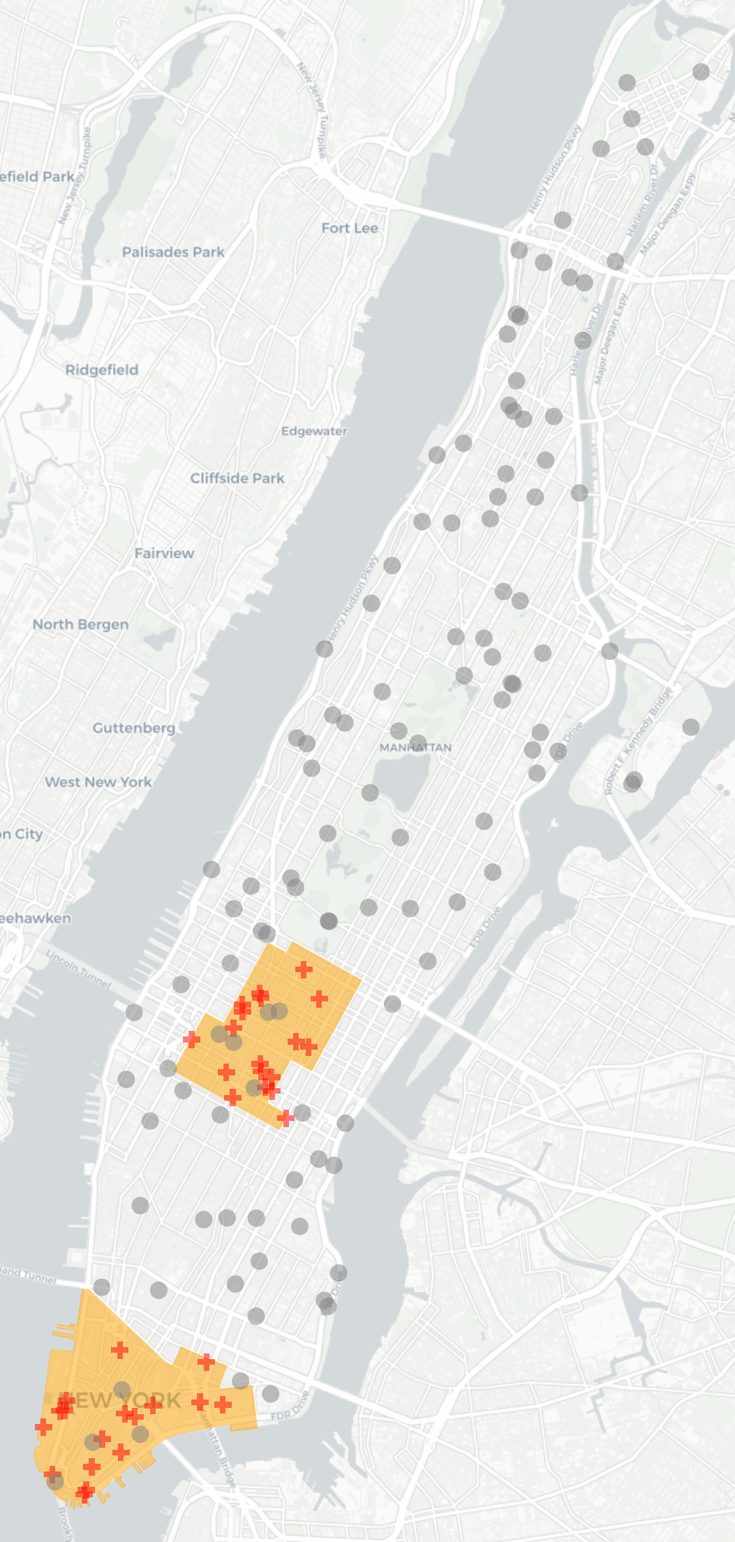
   (a) CVs’ and AVs’ initial locations in Setting 1

   

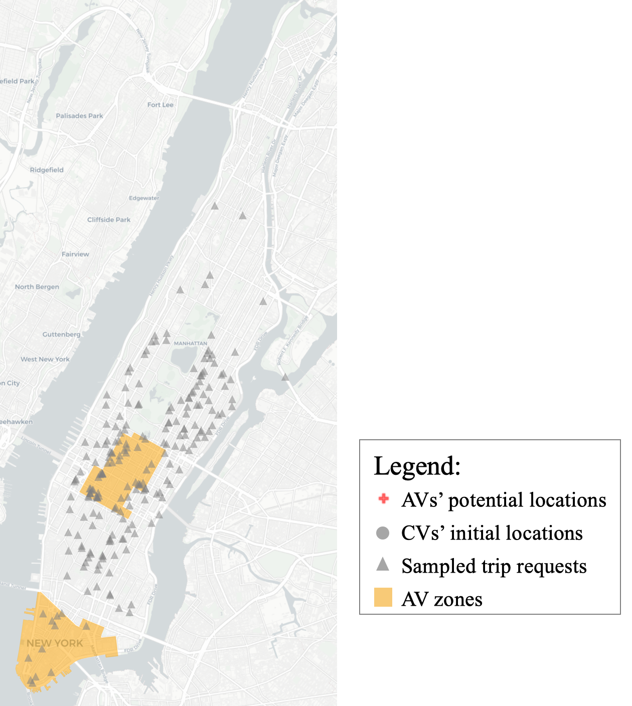
   (b) Request pickup locations in a sampled experiment

   

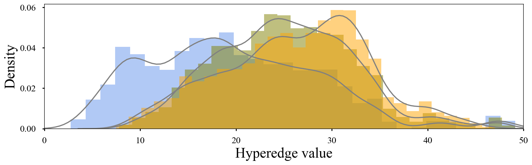
   (c) Sampled hyperedge value distributions in shareability graphs

   Figure 6: High-capacity mixed autonomy traffic experiment in Manhattan, NYC.

2. Supply: The basis set $S_{B}$ represents the CVs with a fixed capacity of two that provides the conventional ride-hailing service.

   • In the high-capacity SRAMF (Setting 1 in Figure 6), the augmented set $S_{A}$ represents the initial locations of automated shuttles fleets that can be redistributed for the regular mobility service. Each shuttle is of capacity up to ten and can only operate within AV zones.

   • In the mid-capacity SRAMF (Setting 2 in Figure 7), the augmented set $S_{A}$ represents a set of locations to preposition taxi-like AVs of capacity three. These locations are sampled from charging stations in NYC from the NREL Alternative Fueling Stations data NREL (2021). The algorithm will choose among $S_{A}$ to position idle AVs for charging before the next assignment.

   

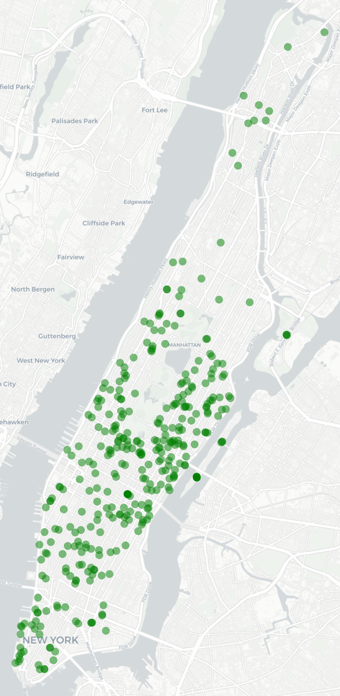
   (a) Public EV charging stations in Manhattan, NYC

   

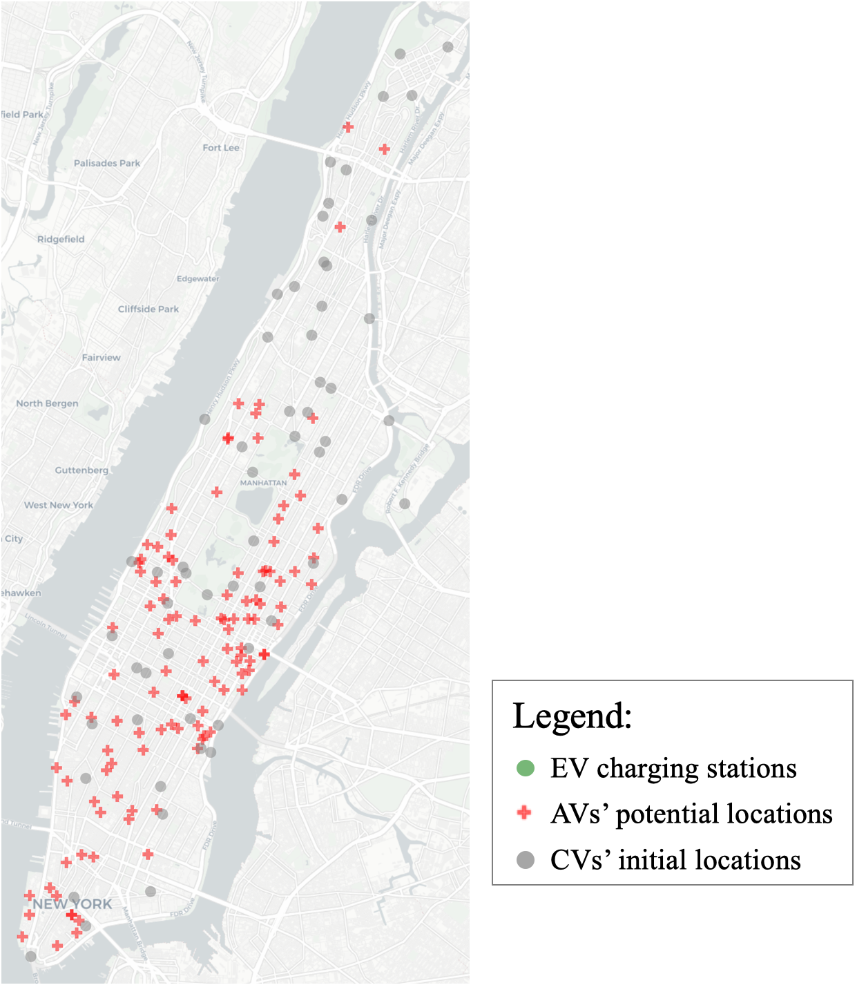
   (b) $S_{A}$ and $S_{B}$ for Setting 2 in a given scenario

   Figure 7: Mid-capacity mixed autonomy traffic experiment in Manhattan, NYC. $S_{A}$ in Figure 7b are randomly chosen from the current EV charging stations (NREL 2021) in Figure 7a.

3. Demand: The trip requests are sampled from the NYC Taxi and Limousine Commission trip data which includes the origin-destination, number of passengers, trip time, and fares (TLC 2021) (Figure 6b).

4. Hyperedge values: The hyperedge cost follows eq.(1). Each trip’s pickup time is computed from the shortest path connecting trip requests on a road network. Customer’s preference over CVs and AVs is randomly generated with $v_{e}>0$ for all hyperedges $e$. $N$ scenarios are independent and identically distributed and used to compare approximation algorithms and the benchmark model (Figure 6c).

5. Time intervals: We consider the rolling-horizon policy with a fixed interval of 15 minutes. This interval allows for repositioning of selected idle vehicles. In addition, many charging stations in NYC are equipped with high-voltage chargers or superchargers, which can restore up to 200 miles in 15 minutes of charging (Xiong et al. 2017).

5.1.2 Assessment of algorithms in the mixed-autonomy simulator.

In both settings, the objective is to choose a subset of $S_{A}$ to reposition these vehicles between trips and maximize the total value of assignments through the rolling horizon, including the values of fulfilled demand, trip costs due to the increasing pickup times, and customers’ preference over the vehicle type in eq.(1). These candidates in $S_{A}$ can be the real-time GPS locations of vehicles (Example 1 or Example 2) or transit stops and parking areas for AVs (Example 3). The solution algorithms select vehicles in each batch at the beginning of each period and determine the trip assignment after all demands are revealed. During preprocessing, the demand forecast model generates $N$ scenarios and constructs the shareability graph using the process in Appendix 8. It generates all hyperedges for the sampled demand as well as the hyperedge values associated with all available vehicles. The hyperedge numbers and other results reported in figures and tables for experiments in this paper are averaged out over all samples.

All computation times are reported from performance on a server with an 18-core 3.1 GHz processor and 192GB RAM. The benchmark model uses a state-of-the-art IP solver (Gurobi 9.1). Setting 1 reports 4-core performance due to the smaller problem size, while Setting 2 is large enough to require the use of all CPU cores. Solving the SRAMF problem in (2) to its optimality by an exact method is impractical considering the massive size of the potential trips. The number of variables in the IP is equal to the product of the number of hyperedges and the sample size, both of which can grow exponentially in real-world applications. The computational time limit is set as six hours per instance. Although the proposed approximation algorithms can handle more extensive networks, our numerical experiments downsample from the taxicab data to keep solvable scales for the benchmark IP solver.

The performance of the proposed approximation algorithm is evaluated under different supply and demand distributions. As the demand profiles are sampled from the taxicab trip data, these algorithms do not depend on any distributional assumption and can be connected to more sophisticated demand forecast models (Geng et al. 2019). The system is tested in both a relatively balanced demand scenario as well as a massive under-supply scenario, with mean numbers of demand across scenarios ranging from $250$, to $4000$, respectively, which are considerably large in a stochastic setting.

Table 1: Parameters in numerical experiments

Setting	AVs (augmented set)			CVs (basis set)			Ratio of demand to supply of vehicles	Number of sampled scenarios
	Capacity	Setup cost	K	Capacity	Setup cost	Vehicle number
Setting 1	5-10	1	5	3	0	115	1.7-2	50
Setting 2	3	1	30-60	2	0	60	35-45	20-30

5.2 Numerical Results for High-Capacity SRAMF

In Setting 1, the proposed algorithm computes the near-optimal solutions for the mixed-autonomy fleet, including selecting AVs and routing vehicles for each sampled demand profile. Figure 8 shows how those chosen AVs (red) and CVs (grey) service trip requests in the face of uncertainty where AVs only operate within the AV zones. The algorithm allocates one AV in the lower AV zone and four AVs in the upper AV zone on the map, which matches the density of demand in Figure 6b.

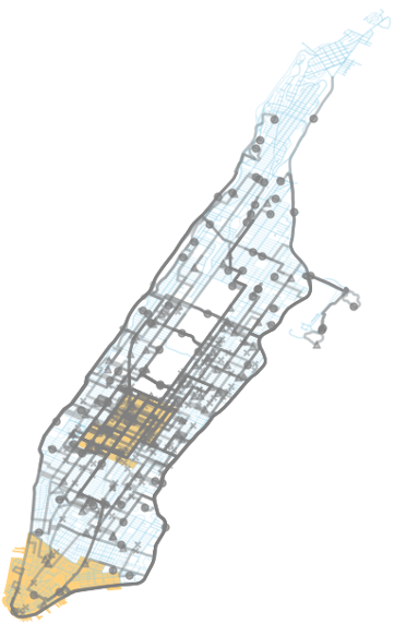
(a) CV routes

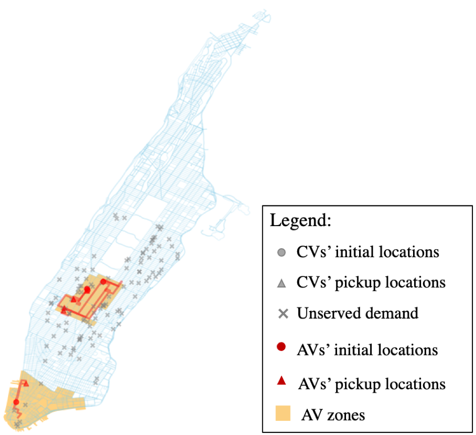
(b) AV routes

Figure 8: Optimal trip assignment and routes in mixed autonomy, high-capacity SRAMF.

The remainder of this section compares two approximation algorithms with a benchmark IP method with regard to the total run times and optimality gap. The computation time comparison is to validate the polynomial-time reduction in terms of the network size, and the optimality-gap comparison is to examine those proved approximation ratios.

5.2.1 Computation times.

The reported computation time includes solving for the near-optimal selection of vehicles and exact assignment in each scenario. Since the same hypergraph is generated beforehand and used throughout all algorithms, we do not report them in this comparison. Two parameters that determine the size of the shareability graph is $|S_{A}|$ (the size of the augmented set) and the number of hyperedges (the number of decision variables in each scenario). Table 2 shows how the total run time grows with the increasing size of the hypergraph. The computation time of LSLPR and MMO algorithms are shown in Table 2.

Note that a significant difference between the proposed algorithms and the exact solver is that these tailored algorithms add vehicles from the set $S_{A}$ sequentially. A parallel-computing scheme can significantly reduce the total run time of approximation algorithms because the evaluation of each scenario can be carried out simultaneously. The exact approach (viz., IP solver) cannot reduce the total run time since it must solve the stochastic program (2) across all samples. The results report the LSLPR and MMO algorithms under a finite-computing-resource (at most eight threads per time) and an infinite-computing-resource setting. The infinite computing resource means that we can evaluate all pairs of vehicles in the active set in LSLPR or the dual variables for all hyperedges in MMO simultaneously. The reported run time is the maximal runtime per iteration. In our experiments, we were able to achieve times close to the reported MMO infinite computing setting, because that can be achieved by evaluating all drivers in $S_{A}\setminus S_{R}$ in parallel. The LSLRP limit is much harder to achieve as the number of potential swaps is combinatorial, however, the computation time will always improve when additional resources are used. The number of hyperedges is the maximum number of hyperedges per scenario.

5.2.2 Optimality gaps.

The optimality gaps of algorithms are compared with the IP benchmark model. Let the objective of the IP solver be $OPT$ and the approximation algorithm’s solution be $ALG$. The optimality gap is measured by $(OPT-ALG)/OPT$. Table 2 shows how the optimality gaps grow with the increasing network size under various supply-demand ratios.

Table 2: Summary of Numerical Results for High-Capacity SRAMF

Demand- supply ratio	$S_{A}$	$S_{B}$	Total # IP variables (hyperedges $\times$ samples)	# of samples	Benchmark	LSLPR			MMO
					IP runtime (second)	LSLPR runtime (8- thread) (second)	LSLPR runtime (max- thread) (second)	Opt. Gap	MMO (8- thread) (second)	MMO (max- thread) (second)	Opt. Gap
1.78	10	115	366550	50	1177	384	20	0.2%	38	16	0.4%
1.78	15	115	372050	50	1332	383	19	0.9%	51	19	0.8%
1.78	20	115	384650	50	1470	337	23	0.7%	58	15	0.8%
1.78	25	115	392500	50	1354	357	24	0.9%	72	26	0.8%
1.78	30	115	403000	50	1464	548	31	0.5%	82	15	0.9%
1.78	35	115	403250	50	1448	599	27	0.4%	97	17	1.0%
1.83	10	115	385450	50	1425	460	29	0.3%	48	15	0.1%
1.83	15	115	407100	50	1516	509	63	0.1%	60	17	0.0%
1.83	20	115	427400	50	1730	449	33	0.5%	77	19	0.3%
1.83	25	115	433950	50	1817	483	35	0.3%	91	22	0.7%
1.83	30	115	458550	50	2027	566	31	0.7%	104	21	0.8%
1.83	35	115	478000	50	2373	565	44	0.5%	137	31	1.2%
1.87	10	115	356250	50	1180	353	26	0.7%	87	65	0.3%
1.87	15	115	375050	50	1350	398	12	0.5%	66	34	0.1%
1.87	20	115	383100	50	1509	455	55	1.0%	78	38	0.1%
1.87	25	115	408650	50	1650	488	18	1.0%	128	70	0.3%
1.87	30	115	427350	50	1690	536	35	1.0%	105	32	0.3%
1.87	35	115	435950	50	1795	535	77	1.3%	141	42	0.3%
1.93	10	115	579800	50	4468	1011	196	0.4%	121	63	0.2%
1.93	15	115	619000	50	6411	1036	58	0.5%	250	140	0.4%
1.93	20	115	651850	50	11243	1237	204	0.2%	224	72	0.3%
1.93	25	115	692250	50	11820	1318	28	0.4%	390	167	0.2%
1.93	30	115	734800	50	5432	1453	99	0.8%	397	86	0.6%
1.93	35	115	845950	50	7038	1830	64	0.6%	516	133	0.4%
2.02	10	115	593200	50	4348	998	50	0.6%	226	182	1.0%
2.02	15	115	662350	50	5843	1792	157	0.2%	175	93	1.0%
2.02	20	115	860950	50	9802	2177	210	0.2%	442	214	1.0%
2.02	25	115	1123050	50	16787	3508	300	0.5%	609	201	0.9%
2.02	30	115	1212400	50	22141	4143	198	0.6%	1234	477	0.4%
2.02	35	115	1243050	50	20920	6327	161	0.4%	1362	487	0.5%

- The demand-supply ratio is the average trip requests over the total number of vehicles ($K+|S_{B}|$); $K=5$.

- 8-thread and max-thread are the number of parallel programs; they are not feasible for the IP benchmark.

- The max-thread runtimes assume enough threads to evaluate all potential swaps or drivers at once:

In LSLRP, max threads = 150; in MMO, max threads = 30.

The overall performance of the proposed approximation algorithms is surprisingly satisfactory. The optimality gap is below 2% throughout all experiments. These results confirm that those approximation ratios proven for the worst-case, $\frac{1}{p^{2}}$ or $\frac{e-1}{(2e+o(1))p\ln p}$, are loose with the real-world trip data. In other words, the performance degradation of these approximation algorithms is negligible when implementing them in shared mobility systems.

5.2.3 Sensitivity analysis.

Three sensitivity analyses conducted in the sensitivity analysis are a) distribution of hyperedge values, b) vehicle number and capacity, and c) sample size. They test how the performance of these approximation algorithms is affected based on changes in input data and model assumptions. We discuss them individually in this section.

Hyperedge value distribution.  The first set of sensitivity analyses aims to check algorithms’ performance degrades with different supply and demand distributions. By replacing the empirical hyperedge values with randomly generated hyperedge values, this analysis examines the robustness of these algorithms. Figure 9 shows the runtime and optimality gaps with uniformly generated hyperedge values (see two distributions in Figure 6c). This uniform distribution represents that the customers’ trust in AV technology is the dominating factor in the hyperedge value such that $v_{e}=\sum_{j\in t}u_{j}+\sum_{j\in t}\tilde{u}_{ij}-c(i,t)\approx\sum_{j\in t}\tilde{u}_{ij}$ for each $e\in E(\xi)$ and the joint utility function follows a uniform distribution.

The runtime of random hyperedge values is smaller than those of real-world data, and the optimality gaps stay low across most instances. This is mainly because the empirical hyperedge values are more concentrated around specific values (i.e., the average trip length). Hence it is more difficult to find the best vehicle from the augmented set. In this case, the local-search-based algorithms are more efficient with more uniformly distributed values.

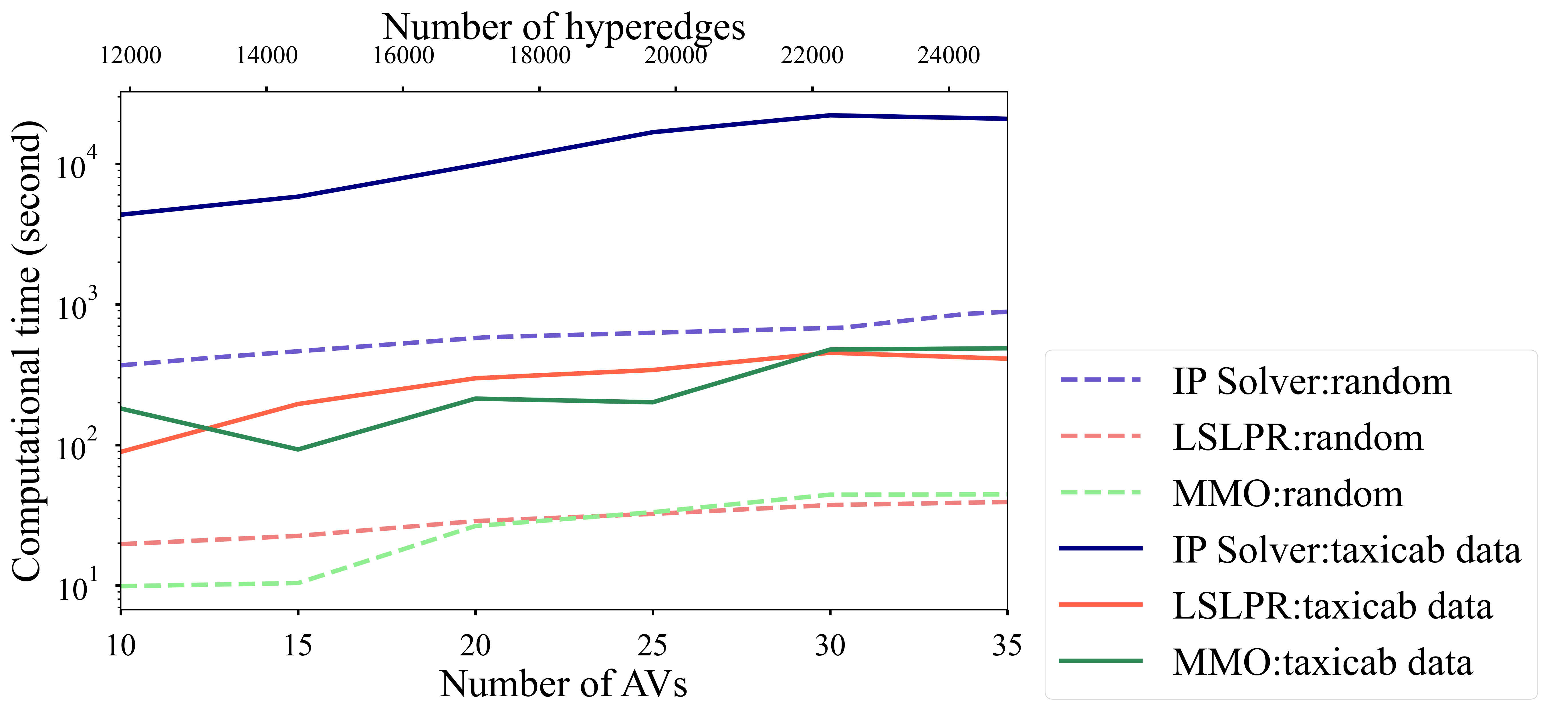
(a) Computation time comparison

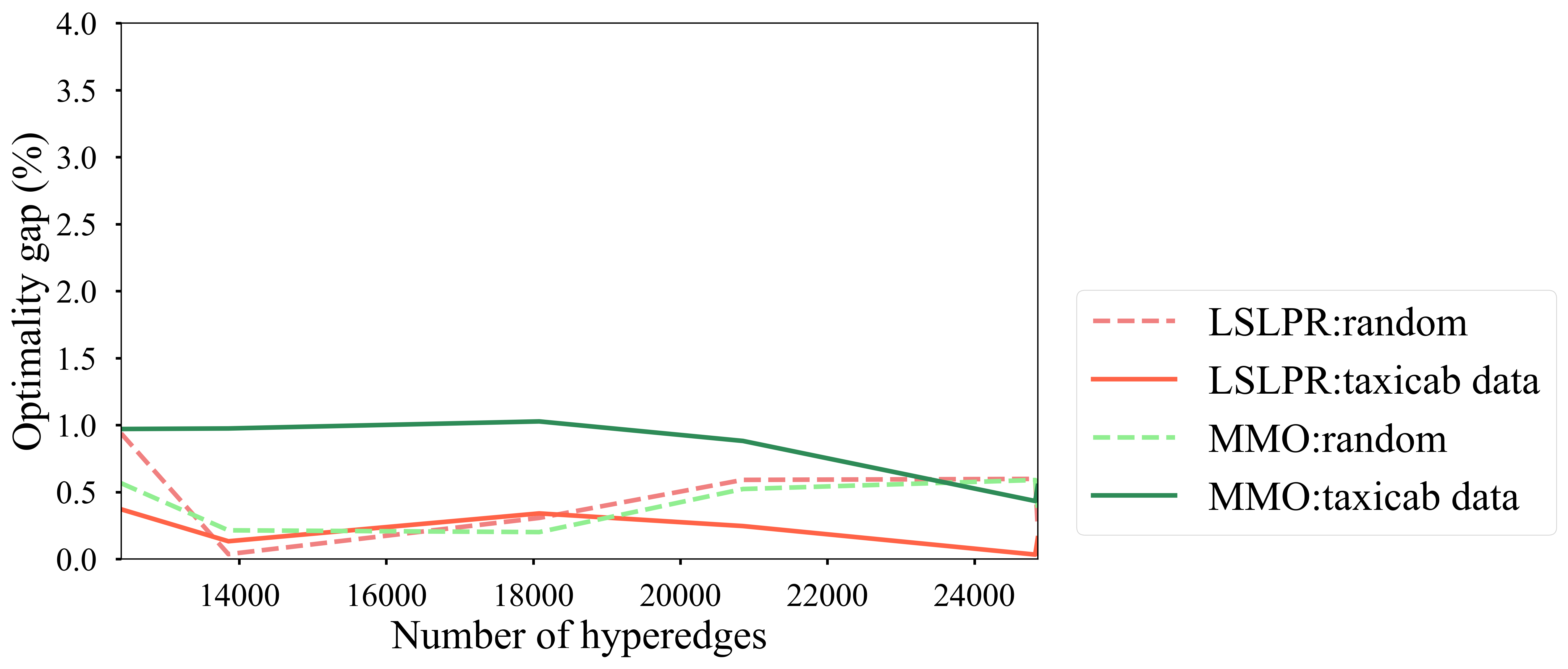
(b) Optimality gap comparison

Figure 9: Impact of input distribution on computation time and optimality gap.

Vehicle capacity.  AVs are the mass transport carriers in the mixed autonomy numerical experiment, whose capacity is up to ten requests and each request may contain more than one passenger. CVs have a fixed capacity of three throughout the experiments. Recall that $p$ bounds the vehicle capacity, Table 3 shows how the vehicle capacity affects the approximation ratios. Observe that the vehicle capacity is not the bottleneck of the performance. Since the number of hyperedges increases with the increasing vehicle capacity, the IP benchmark’s computational time increases. However, we observe that the number of hyperedges plateaus above a certain capacity. This is due to the method of construction of the shareability graph, as described in Section 5.1. In order for a high capacity trip to exist, all subset trips must also exist. This leads to a combinatorially decreasing number of hyperedges with large trip set sizes, unless an even larger set of compatible trips exist. At the density of requests chosen in this experiment in the AV zones, we do not see these large sets of compatible trips. The optimality gaps of both approximation algorithms are not evidently affected by the AV capacity.

Table 3: Impact of vehicle capacity on computation time and optimality gap

Number of AV locations	AV capacity $C_{AV}$	Number of hyperedges	Runtime of IP (second)	Optimality gap of LSLPR (%)	Optimality gap of MMO (%)
35	2	8121	220	0.62	1.12
35	4	11396	288	0.80	0.88
35	6	12048	299	0.99	0.43
35	8	12068	298	1.00	0.03
35	10	12070	301	1.00	0.02

Sample size.  Although SAA guarantees a uniform convergence to the optimal value, it is not clear how the number samples affect the computation times and the optimality gaps. The results of running the same experiments with increasing sample size are summarized in Table 4. This table reports the runtime with unlimited computational resources (i.e., evaluating all scenarios in parallel). The cases with finite multithreading can refer to Figure 6.

Table 4: Impact of sample size on computation time and optimality gap

Number of samples	Number of AV locations	AV capacity	Avg number of hyperedges	Runtime of IP (second)	Runtime of LSLPR (second)	Optimality gap (%)
10	20	5	3100	14	2	3.23
25	20	5	3100	104	5	1.63
50	20	5	3100	445	12	2.03
75	20	5	3100	907	15	2.01
100	20	5	3100	2088	25	0.91
150	20	5	3100	4076	38	3.15
200	20	5	3100	7485	109	1.01

5.3 Numerical Results for Mid-Capacity SRAMF

In Setting 2, a relatively large fleet of electric AVs ($|S_{A}|=114$) and CVs ($|S_{B}|=60$ serve the travel demand in tandem over the entire city area. The results are summarized in Table 5. We also show the optimal assignment and routes in Figure 10.

Table 5: Summary of Numerical Results for Mid-Capacity SRAMF

Demand- supply ratio	S_A	S_B	K	Total # IP variables (hyperedges $\times$ samples)	# of samples	Benchmark	LSLPR			MMO
						IP runtime (second)	LSLPR runtime (36- thread) (second)	LSLPR runtime (max- thread) (second)	Opt. Gap	MMO (36- thread) (second)	MMO (max- thread) (second)	Opt. Gap
22.7	114	60	30	8468768	20	2656	718	213	0.011%	263	87.6	0.11%
34.1	114	60	30	18124448	20	5622	1238	336	0.015%	573	191	0.08%
45.5	114	60	30	31516528	20	8934	3814	2151	0.001%	1050	350	0.05%
22.7	114	60	30	12572544	30	5322	672	267	0.037%	381	127	0.48%
34.1	114	60	30	27495912	30	11559	983	446	0.036%	838	279	0.26%
45.5	114	60	30	47274792	30	19763	1913	1504	0.013%	1457	485	0.14%
22.7	114	60	60	8195056	20	2608	2665	9.26	0.007%	469	227	0.20%
34.1	114	60	60	17905712	20	6277	4898	55.9	0.004%	1022	520	0.11%
45.5	114	60	60	31516528	20	11080	28051	72.0	0.004%	1998	1620	0.076%
22.7	114	60	60	12867024	30	5599	3811	56.7	0.005%	649	544	0.39%
34.1	114	60	60	27147312	30	11220	34360	79.0	0.001%	1516	1210	0.14%
45.5	114	60	60	47274792	30	DNF	DNF	DNF	-	2962	1407	-

- 36-thread and max-thread are the number of parallel programs; they are not feasible for the IP benchmark.

- The max-thread runtimes assume enough threads to evaluate all potential swaps or drivers at once:

In LSLRP, max threads = 3420; in MMO, max threads = 114).

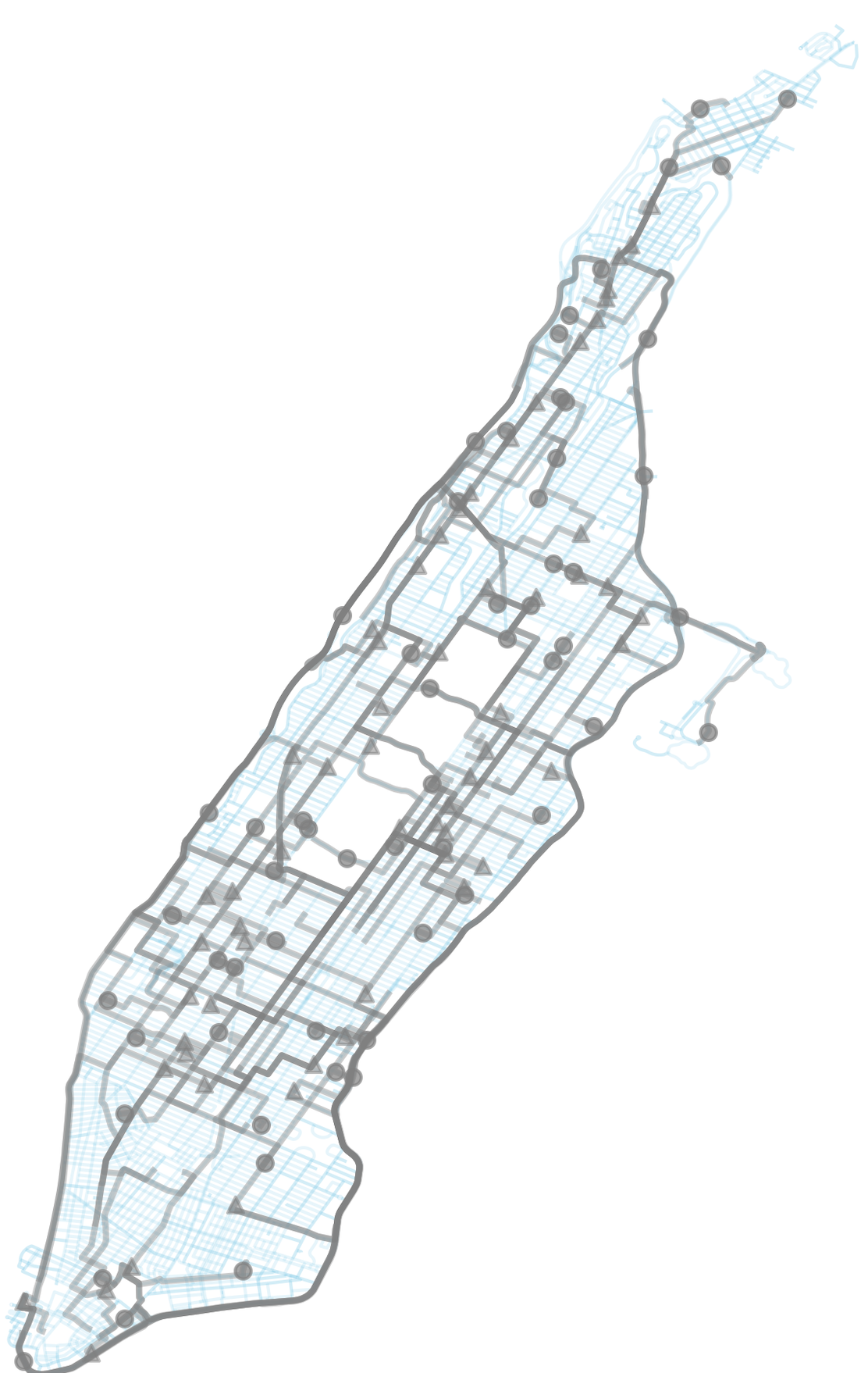
(a) CV routes

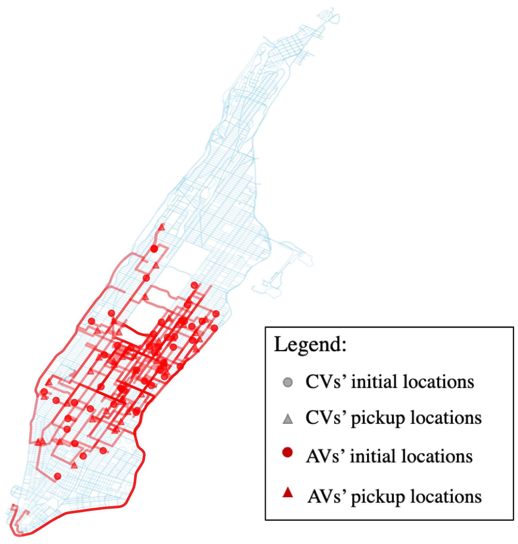
(b) AV routes

Figure 10: Optimal trip assignment and routes in mixed autonomy mid-capacity scenario.

5.3.1 Computation times.

At low sample sizes, the runtime of solving the IP is fairly competitive with the approximation algorithms. Gurobi is a powerful and heavily optimized solver, so this is not very surprising. However, the advantage of MMO and LSLRP at higher sample sizes is clear because they can leverage parallel computation resources.

The runtime of LSLRP varies widely as the swap order greatly affects the runtime. In the $K=60$ case, we occasionally observe very long runtimes for the LSLRP algorithm. This is primarily due to the number of swaps that the algorithm has to evaluate in order to guarantee that it has found a solution. If the algorithm randomly finds a good swap, finding another one that further improves the objective value becomes increasingly difficult. This can lead to the algorithm evaluating a combinatorial number of swaps but the quality of approximation almost attains the optimality.

5.4 Limitations

Since this work focuses on offline algorithms, the limitations of the current experiments include:

1. The system does not allow alternative pickups and dropoffs in trip planning, i.e., the total number of requests is no greater than vehicle capacity in each trip clique.

2. The penalties of balking trips or carryover supply or demand are not directly considered, but can be incorporated into the hyperedge value as discussed in Section 3.1.

The computational time increases linearly with the sample size. The optimality gaps are small across different sample sizes. The algorithm can use a large sample size when the stochasticity in the platform is of major interest and has access to abundant computational resources.

6 Conclusion

SRAMF is a generic formulation for operating shared mobility platforms with blended workforces or mixed autonomy traffic. This paper proposes mid-capacity and high-capacity approximation algorithms for joint fleet sizing and trip assignment in ride-pooling platforms. Widely used real-time ride-pooling frameworks (Alonso-Mora et al. 2017, Simonetto, Monteil, and Gambella 2019) can integrate these approximation algorithms to accelerate the vehicle dispatching process and improve the quality of service with mixed fleets. We give provable guarantees for their worst-case performance and test their average performance in numerical experiments.

To close this paper, we point out several promising future research avenues to address the following limitations. First, we focus on the SRAMF problem in the face of a simple uncertainty structure (i.e., two-stage decision). Since the demand forecast can be time-varying and the vehicle repositioning decisions should adapt to revealing scenarios, extending our framework to a multi-stage setting would be interesting. Second, the construction of hypergraph remains a computational challenge in the worst-case, hence developing efficient reformulation for updated batches of potential matchings may provide computational advantages. Finally, the current trip assignment does not consider cancellation and re-assignment after dispatching vehicles to passengers. Considering these factors in practice may improve the stability of ride-pooling algorithms.

The work described in this paper was partly supported by research grants from the National Science Foundation (CMMI-1854684; CMMI-1904575; CMMI-1940766; CCF-2006778) and Ford-UM Faculty Research Alliance.

7 Summary of Notation

Table 6: Summary of notation and acronyms

Notation	Description
$S_{A}$, $S_{B}$	Augmented set and basis set of vehicles
$\xi$	Randomly generated scenario
$\ell\in[N]$	Index for sampled scenarios and the total number of samples
$D(\xi)$	Set of demand in scenario $\xi$
$E(\xi)$	Set of hyperedges in scenario $\xi$
$G$	Shareability graph, a hypergraph consists of supply and demand vertices and hyperedges
$e$	Each hyperedge $e=\{i,J\}_{i\in S,J\subseteq D}$ is a potential trip where vehicle $i$ serves requests $J$
$u_{j}$	The expected profit of request $j$
$\tilde{u}_{ij}$	Utility gained from matching request $j$ with preferred vehicle type $i$
$c(i,t)$	Travel cost for vehicle $i$ to serve trip $t$
$\alpha$	Approximation ratio
$n$	Total number of vehicles such that $|S_{A}|=n_{A}$ and $|S_{B}|=n_{B}$
$K$	Maximum number of vehicles allowed from the augmented set
$C_{i}$	Capacity of vehicle $i\in S_{A}\cup S_{B}$
$w_{i}$	Number of passengers in request $j$
$p$	Maximum capacity of hyperedge, $p=\max_{i\in S_{A}\cup S_{B}}\{1+C_{i}\}$
$j$	Index for travel demand $j\in D(\xi)$
$w_{j}$	Size of travel demand $j\in D(\xi)$
$E_{i,\xi}$	Set of hyperedges contains vertex $i\in S_{B}\cup S_{R}$ in scenario $\xi$
$t$	Trip is a set of demand following the shortest pickup-and-then-dropoff order
$v_{e}$	Value of hyperedge $e\in E(\xi)$
$nb(e)$	Neighboring hyperedges $e^{\prime}\in E(\xi)$ intersecting with $e$
$x_{e}$	Decision variable for hyperedge $e$, $x_{e}\in\{0,1\}$
$\bar{x}_{e}$	Decision variable for fractional assignment, $x_{e}\in[0,1]$
$y_{i}$	Decision variable for vehicle $i\in[S_{A}]$, $y_{i}\in\{0,1\}$
$v^{*}(\cdot)$	Optimal value of the exact GAP
$Q(y,\xi)$	Optimal value of the assignment in scenario $\xi$
$v_{\max}$	Maximal hyperedge value for all $e\in E$
$v_{\min}$	Minimal hyperedge value for all $e\in E$ such that $v_{e}>0$
$\mathcal{I}$	Independent set as a union of hyperedges satisfying the set-packing constraint
$S_{O}$	Optimal choice of vehicles for SRAMF $S_{O}\subset S_{A}$
$S_{R}$	Choice of vehicles from the algorithm $S_{R}\subset S_{A}$
$\mathcal{L}$	The bijection between $S_{R}$ and $S_{O}$
$\hat{v}(\cdot)$	The objective value of fractional assignment
$\boldsymbol{z}$	Optimal LP solutions to $\hat{v}(S_{O})$
$F_{i}$	Hyperedges intersect with vehicle $i$
$H_{d}$	Hyperedges intersect with demand $d$
$\bot$	Dummy hyperedge in LSLPR
$\Delta_{d}(e,f)$	Decomposition mapping between hyperedge $e$ and $f$
$U_{i_{1}i_{2}}$	Marginal value function with $i_{1}\in S_{R}$ and $i_{2}\in S_{O}$
$\hat{v}_{ON}$	Objective value of the online algorithm
$u_{g,\xi}$	Dual variable in the MMO algorithm for $g\in e$ and scenario $\xi$
$\Gamma_{e}$	$\Gamma_{e}=\sum_{g}u_{g,\xi}$ as the left side of dual constraints
$\boldsymbol{c}_{e}$	Row of cost coefficient in the dual covering problem with entry $c_{e}(g,\xi)$
$M$	The augmented set is partitioned into $M$ subsets
$\epsilon$	Error tolerance (for stopping criteria)
$\delta$	Error tolerance (for sample average approximation) or constant in MMO update subroutine
$OPT$	Optimal value of the SRAMF problem
$ALG$	Objective value of solving SRAMF by approximation algorithms
Acronym	Description
CV/AV	Conventional/automated vehicle
GAP	General assignment problem
LP	Linear program
IP	Integer program
LSLPR	Local-search linear-program-relaxation algorithm
MMO	Max-min online algorithm
SAA	Sample average approximation
SRAMF	Stochastic ride-pooling assignment with mixed fleets
VRP	Vehicle routing problem
DVRP	Dynamic vehicle routing problem

8 Performance Analysis of Construction of Shareability Graphs

The main idea of recent ride-pooling assignment papers (Santi et al. 2014, Alonso-Mora et al. 2017, Simonetto, Monteil, and Gambella 2019) is to separate the problem into two parts: 1) constructing the shareability graph and compatible requests and vehicles, and 2) optimally assigning those trips to vehicles by solving GAP. This paper primarily focuses on algorithms and approximation bounds for the stochastic extension to the second part, but we acknowledge the importance and difficulty of the first task and describe them in detail below for completeness.

8.1 Procedure for Constructing Shareability Graphs

$D(\xi)$ is a set of all trip requests revealed in scenario $\xi$, and this section omits $\xi$ when there is no confusion because the hyperedges for scenarios are generated separately. We consider a number of parameters to be given by the customer or externally dictated to the platform (based on desired service parameters). These include, for each customer $j$, the maximum waiting time, $\omega_{j}$, and allowable delay, $r_{j}$.

• (Constraint I) Travel time from vehicle location to pick-up of customer $j$ in order must be less than $\omega_{j}$.

• (Constraint II) Travel time from origin to destination of customer $j$ in order must be less than $r_{j}$.

Additionally, as defined in the setting, the hyperedge weight consists of three parts: value of trip requests $\sum_{j}u_{j}$, preference of the vehicle type $\tilde{u}_{sj}$, and travel cost of delivering all trip requests in a single trip. We take a three-request clique $(j_{1},j_{2},j_{3})$ as an example. Let $t_{k}=\{O_{j_{1}},O_{j_{2}},\ldots,D_{j_{2}},D_{j_{3}}\}$ be a specific ordered sequence of origins and destinations and $SP(t_{k})$ be the shortest path route connecting them. Let $T_{e}=\cup_{k}t_{k}$. Note that this is slightly less demanding than finding all feasible Hamiltonian paths if we enforce that in all trips, the origins must be picked up before any destination is visited. Let $c(s,e)=\min_{t_{k}\in T_{e}}v(t_{k})$ where $c(t_{k})$ is the cost of serving all requests following the shortest-path $SP(t_{k})$. We define a set function $f(e)$ that takes a hyperedge consisting of a vehicle $s$ and a potential combination of trips, $T_{e}$, as below:

$$f(e)=\begin{cases}0&\text{ if }\forall t_{k}\in T_{e},\,SP(t_{k})\text{ violates constraints I and II}\\ c(s,e)&\text{ otherwise}\end{cases}.$$

The bottleneck of computation time is still finding vehicle routes that satisfy the given constraints by solving a constrained VRP problem, which is NP-hard. Therefore, all heuristic methods can only minimize this bottleneck as much as possible by reducing the number of combinations to check at each step. For example, Ke et al. (2021) suggested a reformulation for finding $c(s,e)$ to avoid enumerating all possible paths.

We combine multiple heuristic methods in literature to construct the shareability graph. First, we need to identify the valid single customer trips for a given vehicle $s$. Let $D_{s}$ be the demand that can be served by vehicle $s$ in a single trip within the allowable pickup time. We may further reduce the number of trips by planning on a spatiotemporal graph and examining compatible trips’ cliques. By testing trips in order of increasing size and only considering a trip if all subsets of trips (where one request is removed from the trip) are feasible, we reduce the number of candidate trips by orders of magnitude. This heuristic generates the shareability graph in Figure 2 in which a set of requests is tested for trip compatibility only if every subset of that set of requests is also compatible.

Lemma 8.1

(Alonso-Mora et al. (2017)) A trip associated with the hyperedge $e$ is feasible for vehicle $s$ only if, for all $j\sim e,j\in D_{s}$, hyperedges (subtrips) $e^{\prime}=e\backslash\{j\}$ are feasible.

The heuristic reduces the candidate hyperedge sets by leveraging the topological relationship between matchable trips of size $k$ and $k+1$ (see Figure 11), without eliminating potentially feasible trips. The hypergraph can then be constructed in order of increasing capacity to minimize the number of request sets tested. Additionally, we adopt the following rules to further reduce the number of candidate trips:

1. Since only hyperedges with nonnegative edge weights are of interest, we remove all the trips from the candidate set subject to $f(e)<=0$.

2. If a vehicle v is not feasible for trip $t_{k}$ at time $\tau$, it will not be feasible for $t_{k}$ at any time $\tau^{\prime}>\tau$ (Liu and Samaranayake 2020).

Let $C_{k}(D)$ be the set of combinations of size $k$ of the elements of the set $D$. This process is summarized as follows:

Data: Vehicle locations and requests (request time, pick-up, drop-off, preferred vehicle type, acceptable delay)

Result: Set of hyperedges, $E$, each containing a vehicle, $s$, and a set of compatible requests for that vehicle to serve in one trip. Hyperedge values are $v_{e}$ for all $e\in E$.

Initialize $E=\varnothing$

for $s\in S_{A}\cup S_{B}$ do

       Identify candidate passengers

       $D_{s}^{1}\leftarrow\{e\in D\mid f((s,e))>0\}$

       Add hyperedges of size one

       $E_{k}\leftarrow\bigcup_{e\in D_{s}^{1}}(s,e)$

       for $k=2,\ldots,c$ do

             for Demand set $d\in C_{k}(D_{s}^{k-1})$ do

                   Add trips of size k if all subsets exist and value greater than 0

                   if $(s,e^{\prime})\in E_{k-1}\forall i\in C_{k-1}(d)$ and $f((s,e^{\prime}))>0$ then

                         $E_{k}\leftarrow E_{k}\cup(s,d)$

                         $D_{s}^{k}\leftarrow D_{s}^{k}\cup d$

                  

            

      

$E=\bigcup_{k=1}^{p-1}E_{k}$

Return hyperedges $E$ and their values $v_{e}$

Algorithm 5 Construction of Shareability Graph

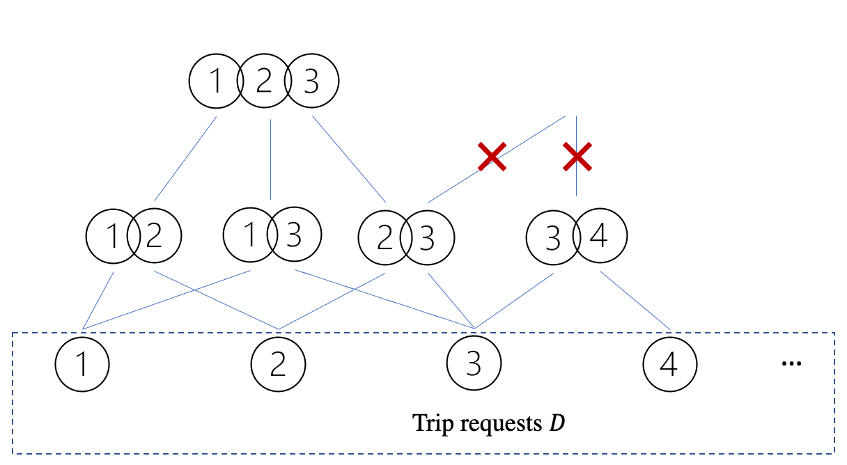
Figure 11: Topological relationship between cliques of matchable requests. In this example, (2,3,4) is not a valid combination of requests because the (2,4) combination was not valid.

8.2 Performance and Complexity Analysis of the Hypergraph Construction Procedure

8.2.1 Optimality analysis.

The two-step ride-pooling assignment that first constructs the hypergraph and then solves GAP obtains the exact optimal solution of solving the joint VRP and enjoys the computational advantage for large fleets. Since this work focuses on stochastic assignment, the optimality analysis does not consider the errors of computing hyperedge values. The following results from Alonso-Mora et al. (2017) provide positive guarantees for returning a feasible set of hyperedges in the shareability graph: without enumerating all trip combinations:

1. $v^{*}$ from solving GAP on the shareability graph obtains the optimal value for ride-pooling for an arbitrary batch of supply and demand.

2. The construction of the shareability graph is anytime optimal, i.e., given additional computational resources, the set of hyperedges is only expanded to allow for improved matching.

The second property guarantees using a capacity bound, the threshold of which is derived below, as an early stopping criterion in generating the hypergraph will still provide satisfactory results. Solving GAP on this reduced shareability graph can guarantee anytime optimality such that the output is near-optimal for the original problem with high probability.

8.2.2 Computational complexity analysis.

We consider a fixed sample of demand $D$ and vehicles $S$ in this section as the hyperedges of each scenario can be generated in parallel. The realized demand has size $|D|=d$.

Lemma 8.2

In the worst case, where all demand is compatible and can be served by all vehicles, the runtime is $O(|S|d^{p-1})$.

While in the worst-case runtime is large, this scenario only arises when all trips are compatible for ride-pooling, which is unlikely in practice. Therefore, we consider the Erdos-Renyi model in which an arbitrary pair of demand is matchable (i.e., satisfy the conditions above) with probability $q$. Empirical studies showed that $q$ was often a small number ($<0.1$) over a large area (Ke et al. 2021).

Lemma 8.3 (Bollobás and Erdös (1976))

The expected number of cliques of size $k$ is ${d\choose k}q^{{k\choose 2}}$.

For example, with $d=1000$ and $q=0.1$, the expected number of cliques of size $3$ (each vehicle deliver at most two requests in a single trip) is $500$. Often we observe the size of complete cliques of compatible trips to be less than 10, our maximum tested capacity, and the total number of hyperedges is manageable.

Lemma 8.4 (Matula (1976))

As $d\rightarrow\infty$, the maximal clique size $\rho$ takes on one of at most two values around $\frac{2\log d}{log1/q}$ with probability tending to one, i.e. with $b=1/q$, $\lfloor 2\log_{b}d\rfloor<\rho<\lceil 2\log_{b}d\rceil$.

Therefore, we only need to consider hyperedges with size less than $p^{*}=\min\{p,\rho+1\}$ (i.e., the height of the cliques’ graph in Figure 11). We have the following theorem for the runtime of constructing shareability graphs.

Theorem 8.5

In the average case that the demand and supply profiles satisfying the random geometric graph conditions, the runtime is $O(|S|d^{p^{*}-1})$.

Proof 8.6

Proof: The expected number of hyperedges connected to vehicle $s$, $E_{s,\max}$, is bounded by

$$E_{s,\max} ={d\choose 1}1^{2}+{d\choose 2}2^{2}q+\dots+{d\choose(p^{*}-1)}(p^{*}-1)^{2}q^{(p^{*}-2)}$$

$$\leq ed+\left(\frac{ed}{2}\right)^{2}2^{2}q+\dots+\left(\frac{ed}{p^{*}-1}\right)^{p^{*}-1}(p^{*}-1)^{2}q^{(p^{*}-2)}$$

$$=ed+\frac{1}{q}\left[\left(\frac{eqd}{2}\right)^{2}2^{2}+\dots+\left(\frac{eqd}{p^{*}-1}\right)^{p^{*}-1}(p^{*}-1)^{2}\right]=O(d^{p^{*}-1}),$$

where $e$ is the Euler’s number.

9 Supplementary Results for Approximation Algorithms

9.1 Proof for Sample Average Approximation in SRAMF

Proof 9.1

Proof: We denote the optimal value of the SRAMF problem (2) as $v^{*}$ and the optimal value of problem for the objective from Algorithm 2 as $\hat{v}(S_{O})$. Let $\delta$ be the upper bound of the optimality gap $v^{*}-\hat{v}(S_{O})$. We assume that $\mathbb{E}[Q(y,\xi)]=\Omega(m^{-2})$ for any $\xi$ where $m$ is a given constant. The main task is to show that:

1. $\mathbb{E}[\hat{v}(S_{O})]=\Omega(m^{2})$ with the sample size $N=\frac{m^{4}}{\delta^{2}}$.

2. $Pr(\hat{v}(S_{O})\notin[(1-\delta)v^{*},(1+\delta)v^{*}])\leq\exp(-\frac{\delta^{2}}{2}\mathbb{E}[\hat{v}(S_{O})])$.

Let $D(\xi)<D$ for all $\xi$. For any selection of vehicles in $S_{A}$ denoted by $y\in Y$, $\mathbb{E}[Q(y,\xi)^{2}]<\infty$, because we can choose $K$ vertices in $S_{A}$ with maximum number of $D$ edges. The upper bound of of hyperedge value $v_{ij}$ is $v_{\max}$. Thus we have $\mathbb{E}[Q(y,\xi)^{2}]<K^{2}|v_{\max}|^{2}D^{2}<\infty$. Without loss of generality, we draw the following observations from the standard stochastic programming literature (Pagnoncelli, Ahmed, and Shapiro 2009):

1. $\hat{v}(S_{O})\to v^{*}$ as $N\to\infty$;

2. $\mathbb{E}[\hat{v}(S_{O})]\geq v^{*}$.

Since $N$ samples are i.i.d., we can use the Chernoff bound on the measure:

$$Pr(\hat{v}(S_{O})\notin[(1-\delta)v^{*},(1+\delta)v^{*}])\leq\exp(-\frac{\delta^{2}}{2}\mathbb{E}[\hat{v}(S_{O})]).$$

Setting $N=m^{4}/\delta^{2}$ and using the assumption that $\mathbb{E}[Q(y,\xi)]=\Omega(m^{-2})$, by Jensen’s inequality, we have:

$$\delta^{2}\mathbb{E}[\hat{v}(S_{O})]\geq\delta^{2}N\cdot E[Q(y,\xi)],$$

i.e., $\delta^{2}\cdot\mathbb{E}[\hat{v}(S_{O})]=\Omega(m^{2})$. We have

$$Pr\Big{(}\hat{v}(S_{O})\notin[(1-\delta)v^{*},(1+\delta)v^{*}]\Big{)}\leq\exp(-\Omega(m^{2})),$$

which achieves the second task as

$${\color[rgb]{0,0,0}Pr\left((\frac{1}{2}-\epsilon)\hat{v}(S_{O})<(\frac{1}{2}-\epsilon)(1-\delta)v^{*}\right)+Pr\left((\frac{1}{2}-\epsilon)\hat{v}(S_{O})>(\frac{1}{2}-\epsilon)(1+\delta)v^{*}\right)}$$

$$\leq Pr\left(\hat{v}(S_{R})<(\frac{1}{2}-\epsilon)(1-\delta)v^{*}\right)+Pr\left(\hat{v}(S_{R})>(\frac{1}{2}-\epsilon)(1+\delta)v^{*}\right)$$

$$\leq \exp(-\Omega(m^{2})).$$

The first inequality is because $\frac{1}{p^{2}}\hat{v}(S_{O})\leq\hat{v}(S_{R})\leq\hat{v}(S_{O})$. This concludes the approximation ratio for LSLPR algorithm for the stochastic counterpart of the ride-pooling problem. $\square$

9.2 Proof for Lemma 4.1

We use a network flow formulation to prove the existence of the mapping $\Delta_{d}:H^{\prime}_{d}\times H^{\prime}_{d}\rightarrow\mathbb{R}_{+}$. Consider a bipartite graph with nodes $L=\{\ell_{e}:e\in H^{\prime}_{d}\}$ and $R=\{r_{f}:f\in H^{\prime}_{d}\}$, and arcs $L\times R$. There is an additional source node $s$, and arcs from $s$ to each $L$-node and arcs from each $R$-node to $s$. Every arc $(i,j)$ in this network has a lower bound $\alpha(i,j)$ and an upper bound $\beta(i,j)$. The goal is to find a circulation $z$ such that $\alpha(i,j)\leq z(i,j)\leq\beta(i,j)$ for all arcs $(i,j)$. Recall that a circulation is an assignment of non-negative values to the arcs of the network so that the in-flow equals the out-flow at every node. The lower/upper bounds are set as follows.

1. For each arc $(i,j)\in L\times R$, we have $\alpha(i,j)=0$ and $\beta(i,j)=\infty$.

2. For each arc $(s,\ell_{e})$ where $e\in H^{\prime}_{d}$, we have $\alpha(s,\ell_{e})=\beta(s,\ell_{e})=x_{e}$.

3. For each arc $(r_{f},s)$ where $f\in H^{\prime}_{d}$, we have $\alpha(r_{f},s)=\beta(r_{f},s)=z_{f}$.

Recall that $\boldsymbol{x}$ and $\boldsymbol{z}$ are the LP solutions corresponding to $\hat{v}(S_{R})$ and $\hat{v}(S_{O})$.

Given any circulation $z$, we define $\Delta_{d}(e,f)=z(\ell_{e},r_{f})$ for all $e,f\in H^{\prime}_{d}$. Then, it is easy to see that all 3 conditions in Lemma 4.6 are satisfied.

It just remains to prove the existence of some circulation. By Hoffman’s circulation theorem (Hoffman 2003), there is a circulation if and only if

$$\alpha\left(\delta^{-}(T)\right)\leq\beta\left(\delta^{+}(T)\right),\qquad\forall T\mbox{ subset of nodes}.$$ (17)

Above, $\delta^{-}(T)$ denotes all arcs from a node outside $T$ to a node inside $T$; similarly, $\delta^{+}(T)$ denotes all arcs from a node inside $T$ to a node outside $T$. This condition can be verified using the following cases:

• $T\cap L\neq\varnothing$ and $T\cap R\neq R$. In this case, there is some arc from $L\times R$ in $\delta^{+}(T)$, so the RHS in (17) is $\infty$, which is clearly satisfies the condition.

• $T\cap L=\varnothing$. If source $s\not\in T$ then $\alpha(\delta^{-}(T))=0$; so (17) is clearly true. If source $s\in T$ then $\beta(\delta^{+}(T))\geq\sum_{e\in H^{\prime}_{d}}x_{e}=1$ as all of $L$ lies outside $T$, and clearly $\alpha(\delta^{-}(T))\leq 1$; so (17) holds.

• $T\cap R=R$. If $s\in T$ then $\alpha(\delta^{-}(T))=0$; so (17) is clearly true. If source $s\not\in T$ then $\beta(\delta^{+}(T))\geq\sum_{f\in H^{\prime}_{d}}z_{f}=1$ as all of $R$ lies inside $T$, and clearly $\alpha(\delta^{-}(T))\leq 1$; so (17) holds.

9.3 Supplementary Results for MMO Algorithm

Recall that $\hat{v}(S_{R})=\sum_{\xi}\hat{v}(S_{R},\xi)$ where $\hat{v}(S_{R},\xi)$ is defined as the LP in (4). So, we can write $\hat{v}(S_{R})$ as the following LP:

$$\hat{v}(S_{R})=\operatorname*{maximize}_{x} \frac{1}{N}\sum_{\xi}\sum_{e\in E(\xi)}v_{e}x^{\xi}_{e}$$ (18)

$$s.t. \sum_{e\in E(\xi):j\in e}x^{\xi}_{e}\leq 1 \forall j\in D(\xi)\quad\forall\xi$$

$$\sum_{e\in E(\xi):i\in e}x^{\xi}_{e}\leq 1 \forall i\in S_{A}\cup S_{B}\quad\forall\xi$$

$$x^{\xi}_{e}=0 \forall e\sim S_{A}\setminus S_{R}\quad\forall\xi$$

$$x^{\xi}_{e}\geq 0 \forall e\in E(\xi)\quad\forall\xi.$$

For any vehicle $i$ and scenario $\xi$, set $F_{i,\xi}\subseteq E(\xi)$ denotes all the hyperedges incident to $i$ in scenario $\xi$. Note that all variables $x^{\xi}_{e}$ with $e\sim S_{A}\setminus S_{R}$ are set to zero. So, it suffices to consider the LP with variables $x^{\xi}_{e}$ for $e\in F_{i,\xi}$ and $i\in S_{B}\cup S_{R}$.

We now consider the dual of the above LP (which has the same optimal value by strong duality). Let $G=S_{A}\cup S_{B}\cup\left(\cup_{\xi}D(\xi)\right)$ denote a combined groundset consisting of all vehicles and demands from all scenarios. The dual variables are $u_{g,\xi}$ for all $g\in G$ and scenarios $\xi$. The dual LP is:

$$\hat{v}(S_{R})\,\,= \,\,\operatorname*{minimize}_{u}\sum_{\xi}\sum_{g\in G}u_{g,\xi}$$

$$s.t.\,\,\sum_{g\in e}u_{g,\xi}\geq\frac{v_{e}}{N}, \forall e\in F_{i,\xi},\quad\forall\xi,\quad\forall i\in S_{R}\cup S_{B}$$

$$\qquad\boldsymbol{u}\geq 0.$$

References

- Alonso-Mora et al. (2017) Alonso-Mora J, Samaranayake S, Wallar A, Frazzoli E, Rus D, 2017 On-demand high-capacity ride-sharing via dynamic trip-vehicle assignment. Proceedings of the National Academy of Sciences 114(3):462–467.
- Arkin and Hassin (1998) Arkin EM, Hassin R, 1998 On local search for weighted k-set packing. Mathematics of Operations Research 23(3):640–648.
- Ashlagi et al. (2018) Ashlagi I, Burq M, Dutta C, Jaillet P, Saberi A, Sholley C, 2018 Maximum weight online matching with deadlines. arXiv preprint arXiv:1808.03526 .
- Benjaafar et al. (2021) Benjaafar S, Wu S, Liu H, Gunnarsson EB, 2021 Dimensioning on-demand vehicle sharing systems. Management Science .
- Bollobás and Erdös (1976) Bollobás B, Erdös P, 1976 Cliques in random graphs. Mathematical Proceedings of the Cambridge Philosophical Society, volume 80, 419–427 (Cambridge University Press).
- Buchbinder et al. (2014) Buchbinder N, Chen S, Gupta A, Nagarajan V, Naor J, 2014 Online packing and covering framework with convex objectives. arXiv preprint arXiv:1412.8347 .
- Castro et al. (2020) Castro F, Frazier P, Ma H, Nazerzadeh H, Yan C, 2020 Matching queues, flexibility and incentives. arXiv preprint arXiv:2006.08863 .
- Chan and Lau (2012) Chan YH, Lau LC, 2012 On linear and semidefinite programming relaxations for hypergraph matching. Mathematical programming 135(1):123–148.
- Chekuri and Khanna (2005) Chekuri C, Khanna S, 2005 A polynomial time approximation scheme for the multiple knapsack problem. SIAM Journal on Computing 35(3):713–728.
- Chen et al. (2017a) Chen D, Ahn S, Chitturi M, Noyce DA, 2017a Towards vehicle automation: Roadway capacity formulation for traffic mixed with regular and automated vehicles. Transportation research part B: methodological 100:196–221.
- Chen et al. (2017b) Chen Z, He F, Yin Y, Du Y, 2017b Optimal design of autonomous vehicle zones in transportation networks. Transportation Research Part B: Methodological 99:44–61.
- Dong and Ibrahim (2020) Dong J, Ibrahim R, 2020 Managing supply in the on-demand economy: Flexible workers, full-time employees, or both? Operations Research 68(4):1238–1264.
- Dong et al. (2021) Dong T, Xu Z, Luo Q, Yin Y, Wang J, Ye J, 2021 Optimal contract design for ride-sourcing services under dual sourcing. Transportation Research Part B: Methodological 146:289–313.
- Erdmann, Dandl, and Bogenberger (2021) Erdmann M, Dandl F, Bogenberger K, 2021 Combining immediate customer responses and car–passenger reassignments in on-demand mobility services. Transportation Research Part C: Emerging Technologies 126:103104.
- Feige et al. (2007) Feige U, Jain K, Mahdian M, Mirrokni V, 2007 Robust combinatorial optimization with exponential scenarios. International Conference on Integer Programming and Combinatorial Optimization, 439–453 (Springer).
- Fleischer et al. (2006) Fleischer L, Goemans MX, Mirrokni VS, Sviridenko M, 2006 Tight approximation algorithms for maximum general assignment problems. Proceedings of the seventeenth annual ACM-SIAM symposium on Discrete algorithm, 611–620.
- Füredi, Kahn, and Seymour (1993) Füredi Z, Kahn J, Seymour PD, 1993 On the fractional matching polytope of a hypergraph. Combinatorica 13(2):167–180.
- Geng et al. (2019) Geng X, Li Y, Wang L, Zhang L, Yang Q, Ye J, Liu Y, 2019 Spatiotemporal multi-graph convolution network for ride-hailing demand forecasting. Proceedings of the AAAI conference on artificial intelligence, volume 33, 3656–3663.
- Gupta and Nagarajan (2014) Gupta A, Nagarajan V, 2014 Approximating sparse covering integer programs online. Mathematics of Operations Research 39(4):998–1011.