Model Reduction of Parametric Differential-Algebraic Systems by Balanced Truncation

Abstract

We deduce a procedure to apply balanced truncation to parameter-dependent differential-algebraic systems. For that we solve multiple projected Lyapunov equations for different parameter values to compute the Gramians that are required for the truncation procedure. As this process would lead to high computational costs if we perform it for a large number of parameters, we combine this approach with the reduced basis method that determines a reduced representation of the Lyapunov equation solutions for the parameters of interest. Residual-based error estimators are then used to evaluate the quality of the approximations. After introducing the procedure for a general class of differential-algebraic systems we turn our focus to systems with a specific structure, for which the method can be applied particularly efficiently. We illustrate the efficiency of our approach on several models from fluid dynamics and mechanics.

We propose a new method that reduces parametric differential-algebraic equations by combining projection methods for differential-algebraic equations and the reduced basis methods for Lyapunov equations. To apply the reduced basis method new error estimators are invented. The performance of our new method is illustrated for several examples.

1 Introduction

In the modeling of various industrial processes one often obtains systems of differential-algebraic equations (DAEs) that are of high dimension. Typical examples are electrical circuits, thermal and diffusion processes, multibody systems, and specific discretized partial differential equations [19, 18]. Often, these systems are further dependent on parameters that can describe physical properties such as material constants and which are often subject to optimization. The resulting parameter-dependent differential-algebraic systems have the form

$$\frac{\mathrm{d}}{\mathrm{d}t}\mathbf{E}(\mu){\mathbf{z}}(t) =\mathbf{A}(\mu)\mathbf{z}(t)+\mathbf{B}(\mu)\mathbf{u}(t),$$ (1a)

$$\mathbf{y}(t) =\mathbf{C}(\mu)\mathbf{z}(t),$$ (1b)

where $\mathbf{E}(\mu),\,\mathbf{A}(\mu)\in\mathbb{R}^{N,N}$, $\mathbf{B}(\mu)\in\mathbb{R}^{N,m}$, and $\mathbf{C}(\mu)\in\mathbb{R}^{p,N}$ are dependent on parameters $\mu\in\mathcal{D}$, where $\mathcal{D}\subset\mathbb{R}^{d}$. The input, the state, and the output are denoted by $\mathbf{u}(t)\in\mathbb{R}^{m}$, $\mathbf{z}(t)\in\mathbb{R}^{N}$ and $\mathbf{y}(t)\in\mathbb{R}^{p}$ for $t\in[0,\infty)$. The matrix $\mathbf{E}(\mu)$ can be a singular. However, throughout this paper, we assume uniform regularity, i. e., the pencil $s\mathbf{E}(\mu)-\mathbf{A}(\mu)$, which is a matrix polynomial in the variable $s$, is assumed to be regular for all $\mu\in\mathcal{D}$, that is $\det(s\mathbf{E}(\mu)-\mathbf{A}(\mu))$ is not the zero polynomial for all $\mu\in\mathcal{D}$. Moreover, we assume that the system under consideration is uniformly asymptotically stable, i. e., the system (or the pencil $s\mathbf{E}(\mu)-\mathbf{A}(\mu)$) is asymptotically stable for all $\mu\in\mathcal{D}$, meaning that all finite eigenvalues of the pencil $s\mathbf{E}(\mu)-\mathbf{A}(\mu)$ have negative real part for all $\mu\in\mathcal{D}$. Throughout the derivations provided in this work we assume that $\mathbf{E}(\cdot)$, $\mathbf{A}(\cdot)$, $\mathbf{B}(\cdot)$, and $\mathbf{C}(\cdot)$ are affine in the parameter $\mu$, i. e.,

$$\begin{split}\mathbf{E}(\mu)&=\mathbf{E}_{0}+\sum_{k=1}^{n_{\mathbf{E}}}\Theta_{k}^{\mathbf{E}}(\mu)\mathbf{E}_{k},\quad\mathbf{A}(\mu)=\mathbf{A}_{0}+\sum_{k=1}^{n_{\mathbf{A}}}\Theta_{k}^{\mathbf{A}}(\mu)\mathbf{A}_{k},\\ \mathbf{B}(\mu)&=\mathbf{B}_{0}+\sum_{k=1}^{n_{\mathbf{B}}}\Theta_{k}^{\mathbf{B}}(\mu)\mathbf{B}_{k},\quad\mathbf{C}(\mu)=\mathbf{C}_{0}+\sum_{k=1}^{n_{\mathbf{C}}}\Theta_{k}^{\mathbf{C}}(\mu)\mathbf{C}_{k},\end{split}$$ (2)

where all $\Theta_{k}^{\mathbf{E}},\,\Theta_{k}^{\mathbf{A}},\,\Theta_{k}^{\mathbf{B}},\,\Theta_{k}^{\mathbf{C}}:\mathcal{D}\to\mathbb{R}$ are parameter-dependent continuous functions and $\mathbf{E}_{k}$, $\mathbf{A}_{k}$, $\mathbf{B}_{k}$, $\mathbf{C}_{k}$ are parameter-independent matrices. For reasons of computational efficiency, we always assume that $n_{\mathbf{E}},\,n_{\mathbf{A}},\,n_{\mathbf{B}},\,n_{\mathbf{C}}\ll N$ and we also assume that the number of inputs and outputs is small compared to the dimension of the states, i. e., $m,\,p\ll N$. For ease of notation, it is sometimes handy to put the matrices $\mathbf{E}_{0}$, $\mathbf{A}_{0}$, $\mathbf{B}_{0}$, and $\mathbf{C}_{0}$ into the sums in (2) and multiply them with the factors $\Theta_{0}^{\mathbf{E}}=\Theta_{0}^{\mathbf{A}}=\Theta_{0}^{\mathbf{B}}=\Theta_{0}^{\mathbf{C}}\equiv 1$. The model (1) is also referred to as the full-order model (FOM). Often, one also considers the input/output mapping of the system in the frequency domain. This relation is typically expressed by the transfer function $\boldsymbol{\mathcal{G}}(\mu,s):=\mathbf{C}(\mu)(s\mathbf{E}(\mu)-\mathbf{A}(\mu))^{-1}\mathbf{B}(\mu).$

Because of the high state-space dimension $N$ of (1) it is useful to apply reduction methods to extract the essential information of the system and its solution. More precisely, we want to determine a (uniformly regular and asymptotically stable) reduced-order model (ROM)

$$\begin{split}\frac{\mathrm{d}}{\mathrm{d}t}\mathbf{E}_{\mathrm{R}}(\mu){\mathbf{z}}_{\mathrm{R}}(t)&=\mathbf{A}_{\mathrm{R}}(\mu)\mathbf{z}_{\mathrm{R}}(t)+\mathbf{B}_{\mathrm{R}}(\mu)\mathbf{u}(t),\\ \mathbf{y}_{\mathrm{R}}(t)&=\mathbf{C}_{\mathrm{R}}(\mu)\mathbf{z}_{\mathrm{R}}(t),\end{split}$$ (3)

with $\mathbf{E}_{\mathrm{R}}(\mu),\,\mathbf{A}_{\mathrm{R}}(\mu)\in\mathbb{R}^{r,r}$, $\mathbf{B}_{\mathrm{R}}(\mu)\in\mathbb{R}^{r,m}$, and $\mathbf{C}_{\mathrm{R}}\in\mathbb{R}^{p,r}$, where $r\ll N$. The reduced state and output are $\mathbf{z}_{\mathrm{R}}(t)\in\mathbb{R}^{r}$ and $\mathbf{y}_{\mathrm{R}}(t)\in\mathbb{R}^{p}$. The aim is to determine the surrogate model in such a way that the output of the ROM well-approximates the output of the FOM for all admissible inputs $\mathbf{u}(\cdot)$ and all parameters $\mu\in\mathcal{D}$. In terms of the transfer function this means that the error $\left\|\boldsymbol{\mathcal{G}}(\mu,\cdot)-\boldsymbol{\mathcal{G}}_{\mathrm{R}}(\mu,\cdot)\right\|$ is sufficiently small in an appropriate norm for all $\mu\in\mathcal{D}$, where $\boldsymbol{\mathcal{G}}_{\mathrm{R}}(\mu,s)$ denotes the transfer function of the ROM.

For parameter-independent problems, i. e.,

$$\mathbf{E}(\mu)\equiv\mathbf{E},\quad\mathbf{A}(\mu)\equiv\mathbf{A},\quad\mathbf{B}(\mu)\equiv\mathbf{B},\quad\mathbf{C}(\mu)\equiv\mathbf{C},\quad\boldsymbol{\mathcal{G}}(\mu,s)\equiv\boldsymbol{\mathcal{G}}(s),$$

there are several classes of model order reduction techniques. Examples are singular value based approaches like balanced truncation [41, 57, 12] and Hankel norm approximations [25]. Additionally, there are Krylov subspace-based methods such as the iterative rational Krylov algorithm (IRKA) [28, 29, 12, 23] and moment matching as well as data-driven methods such as the Loewner framework [39, 26, 9]. Corresponding methods for parameter-dependent systems are introduced in [11, 8, 24].

In this article we focus on balanced truncation which is one of the most popular reduction techniques. This is mainly due to the guaranteed asymptotic stability of the ROM, the existence of an error bound, and appealing numerical techniques for the involved Lyapunov equations [21, 14, 48, 52]. Within balanced truncation, Lyapunov equations corresponding to the original system need to be solved. The solutions of these equations are called Gramians. They describe the input-to-state and state-to-output behavior and are used to construct projection matrices for the reduction. The multiplication of the system matrices with these projection matrices then results in a ROM.

All the above-mentioned methods focus on the case $\mathbf{E}=I_{N}$ and are, however, not directly applicable in the DAE case. Even if the problem is not parameter-dependent, there are several challenges that one has to face (here we assume for simplicity, that the problem is parameter-independent):

1. Since the matrix $\mathbf{E}$ is typically singular, the transfer function $\boldsymbol{\mathcal{G}}(s)$ is possibly improper, i. e., it may have a polynomial part which is unbounded for growing values of $|s|$. If the reduced transfer function $\boldsymbol{\mathcal{G}}_{\mathrm{R}}(s)$ does not match this polynomial part, then the error transfer function $\boldsymbol{\mathcal{G}}(s)-\boldsymbol{\mathcal{G}}_{\mathrm{R}}(s)$ is not an element of the rational Hardy spaces $\mathcal{RH}_{\infty}^{p,m}$ or $\mathcal{RH}_{2}^{p,m}$ (see, e. g, [63] for a definition) and the output error cannot be bounded by the input norm. Thus, a model reduction scheme for DAEs must preserve the polynomial part of its transfer function. This is addressed in [40, 54, 29].

2. In balanced truncation, one has to solve two large-scale Lyapunov equations. In the DAE case, one has to consider a generalization of these – so-called projected Lyapunov equations. Thereby, the Lyapunov equations are projected onto the left and right deflating subspaces corresponding to the finite or infinite eigenvalues of the matrix pencil $s\mathbf{E}-\mathbf{A}$. This involves specific projectors which are hard to form explicitly and that might destroy the sparsity structure of the coefficient matrices. However, for DAE systems of special structure, the projectors are of a particular form which can be exploited from the numerical point of view. For details, we refer to [56, 31, 47, 13].

Besides the approaches mentioned above, some of the issues in model reduction of DAEs are also addressed in [1, 5]. There, the authors introduce an index-aware model order reduction scheme that splits the DAE system into a differential and an algebraic part. However, in this method it is often difficult to maintain sparsity of the system matrices, and hence, it is in general not feasible for many systems with large dimensions. Also data-driven approaches have been recently extended to differential-algebraic systems, see, e. g., [3, 27]. Finally, we would like to mention [15] which provides an overview of model order reduction for DAE systems.

Different approaches for parametric model reduction have been developed as well. Besides others, there exist two main classes of such methods. First, one could determine global bases for the projection spaces for the entire parametric model, e. g., by concatenating the local bases for different parameter values, see, e. g., [7]. Second, there exist approaches for constructing local bases for a specific parameter value by combining local basis information of several prereduced models at different parameter values, e. g., by interpolating between different models [22, 24]. We also refer to [10] for an extensive survey on such methods.

However, to the best of our knowledge, none of the techniques presented in [10] has already been extended to the case of DAE systems. Therefore, the motivation of this paper is to develop a first method for this purpose based on balanced trunction. If we aim to reduce a parameter-dependent system by balanced truncation in a naive fashion, we would have to solve the Lyapunov equations for each individual parameter of interest which is computationally prohibitive. To avoid these computational costs, for the case $\mathbf{E}=I_{N}$, the authors in [51] apply some interpolation techniques to approximate the Gramians for all admissible parameters. The authors in [52], on the other hand, apply the reduced basis method which is a well-established method to reduce parameter-dependent partial differential equations [32, 45]. Using this method, the authors determine the approximate subspaces in which the solutions of the corresponding Lyapunov equations are contained in.

In this paper we extend the reduced basis method to the case of DAE systems where the parametric projected Lyapunov equations are only solved for few sampling parameters. Then, based on these solutions, a reduced subspace in which the Lyapunov equation solutions for all $\mu\in\mathcal{D}$ approximately live, is constructed. The latter steps form the computationally expensive offline phase. After that, using the reduced basis representation, the Lyapunov equations can be solved much more efficiently for all $\mu\in\mathcal{D}$ in the online phase. A crucial question in the offline phase is the choice of the sample parameters. Usually, a grid of test parameters is selected. For these, the error is quantified using a posteriori error estimators. Then new samples are taken at those parameters at which the error estimator estimates the largest error.

In this paper we generalize the reduced basis balanced truncation method of [52] to differential-algebraic systems with a focus on structured systems from specific application areas. The main problems we solve in this paper are the following:

1. We derive error estimators for parameter-dependent projected Lyapunov equations. These can be improved if the given system is uniformly strictly dissipative. Since this condition is not always satisfied, we discuss transformations to achieve this for systems of a particular index 3 structure.

2. We discuss in detail how the polynomial part of parameter-dependent transfer functions of DAE systems can be extracted by efficiently approximating their Markov parameters.

3. We apply this approach to several application problems and illustrate its effectiveness.

Our method also follows the paradigm of decomposing the procedure into an offline and online phase. In the offline phase we approximate the image spaces of controllability and obervability Gramians that are the solutions of projected Lyapunov equations. These approximate image spaces are then used in the online phase, to determine approximations of the Gramians, and hence, the reduced order model, efficiently for all required parameters. The online phase can be performed for any parameter $\mu\in\mathcal{D}$. Due to the reduced dimension obtained by the offline phase, this step is very fast and can be performed repeatedly for all required parameters. Moreover, in this work, we introduce new error estimators, which are used in the offline phase to assess the quality of the reduction.

This paper is organized as follows. In Section 2, two model problems are introduced that motivate the method presented in this paper. In Section 3, we review existing concepts and approaches that will be used later in this paper. Thereby, in Subsection 3.1, we recall projection techniques to decouple the differential and algebraic equations in (1). Afterwards, in Subsection 3.2, we consider model order reduction by balanced truncation for DAE systems. We further address the numerical challenges that arise in computing the solutions of the required Lyapunov equations. Since solving Lyapunov equations for every requested parameter leads to high computational costs, in Section 4 the reduced basis method is presented, which was first applied to standard Lyapunov equations in [52]. We derive two error estimators for our method, one of them is motivated by the estimator from [52], the other one is an adaption of the estimator presented in [48]. Here we also discuss the treatment of the algebraic part of the system that may lead to polynomial parts in the transfer function. Finally, in Section 5, we evaluate the method of this paper by applying it to our model problems from Section 2.

2 Model problems

2.1 Problem 1: Stokes-like DAEs

The first example is the system

$$\begin{split}\frac{\mathrm{d}}{\mathrm{d}t}\begin{bmatrix}E(\mu)&0\\ 0&0\end{bmatrix}\begin{bmatrix}x(t)\\ {\lambda}(t)\end{bmatrix}&=\begin{bmatrix}A(\mu)&G(\mu)\\ G(\mu)^{\mathrm{T}}&0\end{bmatrix}\begin{bmatrix}x(t)\\ \lambda(t)\end{bmatrix}+\begin{bmatrix}B_{1}(\mu)\\ B_{2}(\mu)\end{bmatrix}u(t),\\ y(t)&=\begin{bmatrix}C_{1}(\mu)&C_{2}(\mu)\end{bmatrix}\begin{bmatrix}x(t)\\ \lambda(t)\end{bmatrix},\end{split}$$ (4)

which arises, e. g., if we discretize the incompressible Navier-Stokes equation. The parameter-independent version is presented in [40, 54]. The system matrices are dependent on a parameter $\mu\in\mathcal{D}$, where $\mathcal{D}\subset\mathbb{R}^{d}$ is the parameter domain. For fluid-flow problems, the matrices $E(\mu),\,A(\mu)\in\mathbb{R}^{n,n}$ represent the masses and the discretized Laplace operator. Naturally, it holds that $E(\mu)=E(\mu)^{\mathrm{T}}>0$ and $A(\mu)=A(\mu)^{\mathrm{T}}<0$ for all $\mu\in\mathcal{D}$, where $H>0$ ($H\geq 0$) denotes a positive (semi)definite matrix $H$ and correspondingly $H<0$ ($H\leq 0$) denotes a negative (semi)definite matrix. The discrete gradient is given by $G(\mu)\in\mathbb{R}^{n,q}$ which we assume to be of full column rank for all $\mu\in\mathcal{D}$. The matrices $B_{1}(\mu)\in\mathbb{R}^{n,m},\,B_{2}(\mu)\in\mathbb{R}^{q,m}$ and $C_{1}(\mu)\in\mathbb{R}^{p,n},\,C_{2}(\mu)\in\mathbb{R}^{p,q}$ are the input and the output matrices, respectively. The state of the system at time $t$ is given by $x(t)\in\mathbb{R}^{n}$ and $\lambda(t)\in\mathbb{R}^{q}$. The vectors $u(t)\in\mathbb{R}^{m}$ and $y(t)\in\mathbb{R}^{p}$ are the input and output of the system.

In view of (2) we assume that the symmetry and definitess of $E(\cdot)$ and $A(\cdot)$ is represented in the affine parameter structure as

$$E(\mu)=\sum_{k=0}^{n_{E}}\Theta_{k}^{E}(\mu)E_{k}\quad\text{and}\quad A(\mu)=\sum_{k=0}^{n_{A}}\Theta_{k}^{A}(\mu)A_{k},$$

where $\Theta_{k}^{E}(\cdot)$, $\Theta_{k}^{A}(\cdot)$ are positive parameter-dependent continuous functions with the convention $\Theta_{0}^{E}=\Theta_{0}^{A}\equiv 1$. Furthermore, $E_{0}=E_{0}^{\mathrm{T}}>0$, $A_{0}=A_{0}^{\mathrm{T}}<0$, $E_{k}=E_{k}^{\mathrm{T}}\geq 0$, $A_{k}=A_{k}^{\mathrm{T}}\leq 0$ for $k\geq 1$ are parameter-independent matrices. Moreover, for reasons of computational efficiency, we always assume that $n_{E},\,n_{A}\ll n$.

2.2 Problem 2: Mechanical systems

The second system we consider is of the form

$$\begin{split}\frac{\mathrm{d}}{\mathrm{d}t}\begin{bmatrix}I_{n_{x}}&0&0\\ 0&M(\mu)&0\\ 0&0&0\end{bmatrix}\begin{bmatrix}x_{1}(t)\\ x_{2}(t)\\ \lambda(t)\end{bmatrix}&=\begin{bmatrix}0&I_{n_{x}}&0\\ -K(\mu)&-D(\mu)&G(\mu)\\ G(\mu)^{\mathrm{T}}&0&0\end{bmatrix}\begin{bmatrix}x_{1}(t)\\ x_{2}(t)\\ \lambda(t)\end{bmatrix}+\begin{bmatrix}0\\ B_{x}(\mu)\\ 0\end{bmatrix}u(t),\\ y(t)&=\begin{bmatrix}C_{x}(\mu)&0&0\end{bmatrix}\begin{bmatrix}x_{1}(t)\\ x_{2}(t)\\ \lambda(t)\end{bmatrix},\end{split}$$ (5)

which results from a linearization of the spring-mass-damper model presented in [40]. The mass, damping, and stiffness matrices $M(\mu),\,D(\mu),\,K(\mu)\in\mathbb{R}^{n_{x},n_{x}}$ are assumed to be symmetric and positive definite for all $\mu\in\mathcal{D}$. The matrices $B_{x}(\mu)\in\mathbb{R}^{n_{x},m}$ and $C_{x}(\mu)\in\mathbb{R}^{p,n_{x}}$ are the input and the output matrices. The matrix $G(\mu)\in\mathbb{R}^{n_{x},q}$ reflects algebraic constraints on the system and is of full column rank. In this example, the state includes the displacement $x_{1}(t)\in\mathbb{R}^{n_{x}}$, the velocity $x_{2}(t)\in\mathbb{R}^{n_{x}}$, and Lagrange multiplier $\lambda(t)\in\mathbb{R}^{q}$.

For convenience, we also define

$$\begin{split}E(\mu)&:=\begin{bmatrix}I_{n_{x}}&0\\ 0&M(\mu)\end{bmatrix},\quad A(\mu):=\begin{bmatrix}0&I_{n_{x}}\\ -K(\mu)&-D(\mu)\end{bmatrix},\quad B(\mu):=\begin{bmatrix}0\\ B_{x}(\mu)\end{bmatrix},\\ C(\mu)&:=\begin{bmatrix}C_{x}(\mu)&0\end{bmatrix},\quad n:=2n_{x}.\end{split}$$ (6)

Then with this notation, we can write the mechanical system similarly as in (4) with the difference that the off-diagonal blocks of the state matrix are not the transposes of each other.

Similarly to the first model problem, we assume that $M(\cdot)$, $D(\cdot)$, and $K(\cdot)$ can be written as

$$M(\mu)=\sum_{k=0}^{n_{M}}\Theta_{k}^{M}(\mu)M_{k},\quad D(\mu)=\sum_{k=0}^{n_{D}}\Theta_{k}^{D}(\mu)D_{k},\quad\text{and}\quad K(\mu)=\sum_{k=0}^{n_{K}}\Theta_{k}^{K}(\mu)K_{k},$$

where $\Theta_{k}^{M}(\cdot)$, $\Theta_{k}^{D}(\cdot)$, $\Theta_{k}^{K}(\cdot)$ are positive parameter-dependent continuous functions using the convention $\Theta_{0}^{M}=\Theta_{0}^{D}=\Theta_{0}^{K}\equiv 1$. Furthermore, $M_{0}=M_{0}^{\mathrm{T}}>0$, $D_{0}=D_{0}^{\mathrm{T}}>0$, $K_{0}=K_{0}^{\mathrm{T}}>0$ and $M_{k}=M_{k}^{\mathrm{T}}\geq 0$, $D_{k}=D_{k}^{\mathrm{T}}\geq 0$, $K_{k}=K_{k}^{\mathrm{T}}\geq 0$ for $k\geq 1$ are parameter-independent matrices with $n_{M},\,n_{D},\,n_{K}\ll n_{x}$.

3 Preliminaries

3.1 Decoupling of differential and algebraic equations

In this section we briefly describe the projection technique for decoupling the algebraic constraints in DAEs of the form (1) from the remaining differential equations for a fixed parameter $\mu\in\mathcal{D}$ and under the assumptions of regularity and asymptotic stability. Therefore, for simplicity of presentation, we omit $\mu$ in this section. The details of this can be found in [54, 55, 31, 47].

As shown in [17] there exist regular matrices $\mathbf{W},\leavevmode\nobreak\ \mathbf{T}\in\mathbb{R}^{N,N}$ that transform the system matrices into quasi-Weierstraß form, that is

$$\mathbf{E}=\mathbf{W}\begin{bmatrix}I_{N_{\mathrm{f}}}&0\\ 0&\mathbf{N}\end{bmatrix}\mathbf{T},\qquad\mathbf{A}=\mathbf{W}\begin{bmatrix}\mathbf{J}&0\\ 0&I_{N_{\infty}}\end{bmatrix}\mathbf{T},$$ (7)

where $\mathbf{J}\in\mathbb{R}^{{N_{\mathrm{f}}},{N_{\mathrm{f}}}}$ and $\mathbf{N}\in\mathbb{R}^{N_{\infty},N_{\infty}}$ is nilpotent with nilpotency index $\nu$ that coincides with the (Kronecker) index of the DAE system (1). Here, ${N_{\mathrm{f}}}$ is the number of the finite eigenvalues of the matrix pencil $s\mathbf{E}-\mathbf{A}$ and $N_{\infty}$ is the number of the infinite ones. Accordingly, spectral projectors onto the left and right deflating subspace of $s\mathbf{E}-\mathbf{A}$ corresponding to the ${N_{\mathrm{f}}}$ finite eigenvalues are defined as

$$\boldsymbol{\Pi}_{\mathrm{l}}:=\mathbf{W}\begin{bmatrix}I_{N_{\mathrm{f}}}&0\\ 0&0\end{bmatrix}\mathbf{W}^{-1},\qquad\boldsymbol{\Pi}_{\mathrm{r}}:=\mathbf{T}^{-1}\begin{bmatrix}I_{N_{\mathrm{f}}}&0\\ 0&0\end{bmatrix}\mathbf{T}.$$

We define

$$\mathbf{F}_{\mathbf{J}}(t) :=\mathbf{T}^{-1}\begin{bmatrix}\mathrm{e}^{\mathbf{J}t}&0\\ 0&0\end{bmatrix}\mathbf{W}^{-1},\quad t\in\mathbb{R}\qquad\text{and}$$

$$\mathbf{F}_{\mathbf{N}}(k) :=\mathbf{T}^{-1}\begin{bmatrix}0&0\\ 0&-\mathbf{N}^{k}\end{bmatrix}\mathbf{W}^{-1},\quad k=0,\,\dots,\,\nu-1$$

to derive the states

$$\mathbf{z}_{\mathrm{p}}(t):=\int_{0}^{t}\mathbf{F}_{\mathbf{J}}(t-\tau)\mathbf{B}\mathbf{u}(\tau)\,\mathrm{d}\tau,\qquad\mathbf{z}_{\mathrm{i}}(t):=\sum_{k=0}^{\nu-1}\mathbf{F}_{\mathbf{N}}(k)\mathbf{B}\mathbf{u}^{(k)}(t),$$

under the assumption that the input $\mathbf{u}(\cdot)$ is sufficiently smooth and that the consistency conditions are satisfied, i. e., we assume that $\mathbf{z}_{\mathrm{i}}(0):=\sum_{k=0}^{\nu-1}\mathbf{F}_{\mathbf{N}}(k)\mathbf{B}\mathbf{u}^{(k)}(0)$. They satisfy $\mathbf{z}(t)=\mathbf{z}_{\mathrm{p}}(t)+\mathbf{z}_{\mathrm{i}}(t)$ such that $\mathbf{z}(t)$ solves equation (1a). We refer to $\mathbf{z}_{\mathrm{p}}(t)$ and $\mathbf{z}_{\mathrm{i}}(t)$ as differential and algebraic states. These states are associated with the proper and improper controllability Gramians

$$\mathbf{P}_{\mathrm{p}}=\int_{0}^{\infty}\mathbf{F}_{\mathbf{J}}(t)\mathbf{B}\mathbf{B}^{\mathrm{T}}\mathbf{F}_{\mathbf{J}}(t)^{\mathrm{T}}\,\mathrm{d}t,\qquad\mathbf{P}_{\mathrm{i}}=\sum_{k=0}^{\nu-1}\mathbf{F}_{\mathbf{N}}(k)\mathbf{B}\mathbf{B}^{\mathrm{T}}\mathbf{F}_{\mathbf{N}}(k)^{\mathrm{T}},$$ (8)

respectively. They span the reachable subspaces of the differential and algebraic states. Analogously, the proper and improper observability Gramians

$$\mathbf{Q}_{\mathrm{p}}=\int_{0}^{\infty}\mathbf{F}_{\mathbf{J}}(t)^{\mathrm{T}}\mathbf{C}^{\mathrm{T}}\mathbf{C}\mathbf{F}_{\mathbf{J}}(t)\,\mathrm{d}t,\qquad\mathbf{Q}_{\mathrm{i}}=\sum_{k=0}^{\nu-1}\mathbf{F}_{\mathbf{N}}^{\mathrm{T}}(k)\mathbf{C}^{\mathrm{T}}\mathbf{C}\mathbf{F}_{\mathbf{N}}(k)$$

span the corresponding observability spaces. The proper Gramians are obtained by solving the projected continuous-time Lyapunov equations

$$\mathbf{E}\mathbf{P}_{\mathrm{p}}\mathbf{A}^{\mathrm{T}}+\mathbf{A}\mathbf{P}_{\mathrm{p}}\mathbf{E}^{\mathrm{T}} =-\boldsymbol{\Pi}_{\mathrm{l}}\mathbf{B}\mathbf{B}^{\mathrm{T}}\boldsymbol{\Pi}_{\mathrm{l}}^{\mathrm{T}},\qquad\mathbf{P}_{\mathrm{p}}=\boldsymbol{\Pi}_{\mathrm{r}}\mathbf{P}_{\mathrm{p}}\boldsymbol{\Pi}_{\mathrm{r}}^{\mathrm{T}},$$ (9)

$$\mathbf{E}^{\mathrm{T}}\mathbf{Q}_{\mathrm{p}}\mathbf{A}+\mathbf{A}^{\mathrm{T}}\mathbf{Q}_{\mathrm{p}}\mathbf{E} =-\boldsymbol{\Pi}_{\mathrm{r}}^{\mathrm{T}}\mathbf{C}^{\mathrm{T}}\mathbf{C}\boldsymbol{\Pi}_{\mathrm{r}},\qquad\mathbf{Q}_{\mathrm{p}}=\boldsymbol{\Pi}_{\mathrm{l}}^{\mathrm{T}}\mathbf{Q}_{\mathrm{p}}\boldsymbol{\Pi}_{\mathrm{l}}$$ (10)

and the improper ones by solving the discrete-time Lyapunov equations

$$\mathbf{A}\mathbf{P}_{\mathrm{i}}\mathbf{A}^{\mathrm{T}}-\mathbf{E}\mathbf{P}_{\mathrm{i}}\mathbf{E}^{\mathrm{T}} =(I_{N}-\boldsymbol{\Pi}_{\mathrm{l}})\mathbf{B}\mathbf{B}^{\mathrm{T}}(I_{N}-\boldsymbol{\Pi}_{\mathrm{l}})^{\mathrm{T}},\qquad 0=\boldsymbol{\Pi}_{\mathrm{r}}\mathbf{P}_{\mathrm{i}}\boldsymbol{\Pi}_{\mathrm{r}}^{\mathrm{T}},$$ (11)

$$\mathbf{A}^{\mathrm{T}}\mathbf{Q}_{\mathrm{i}}\mathbf{A}-\mathbf{E}^{\mathrm{T}}\mathbf{Q}_{\mathrm{i}}\mathbf{E} =(I_{N}-\boldsymbol{\Pi}_{\mathrm{r}})^{\mathrm{T}}\mathbf{C}^{\mathrm{T}}\mathbf{C}(I_{N}-\boldsymbol{\Pi}_{\mathrm{r}}),\qquad 0=\boldsymbol{\Pi}_{\mathrm{l}}^{\mathrm{T}}\mathbf{Q}_{\mathrm{i}}\boldsymbol{\Pi}_{\mathrm{l}}.$$ (12)

In Subsection 3.2.2 we will describe how these projected Lyapunov equations can be solved.

In practice, the projectors $\boldsymbol{\Pi}_{\mathrm{l}}$ and $\boldsymbol{\Pi}_{\mathrm{r}}$ are computationally expensive to form and even more expensive to compute with as they are dense matrices of large dimension in general. To determine them, the derivations from [34] can be applied, however they are not numerically stable since a Jordan canonical form needs to be computed. On the other hand, the methods presented in [4], [20], or [37] might be used to generate the differential and algebraic state spaces, however, they involve the determination of matrix kernels which are based on matrix decompositions. Suitable parts of the matrices involved in these decompositions are then used to determine the projection matrices $\boldsymbol{\Pi}_{\mathrm{l}}$ and $\boldsymbol{\Pi}_{\mathrm{r}}$. They are in general not of a sparse structure and, therefore, not applicable if we consider matrices of large dimensions. Hence, if possible, it is advantageous to determine the projection matrices analytically. In many application fields this is possible because the matrices $\mathbf{E}$ and $\mathbf{A}$ are of special structure that can be utilized for this purpose. The examples in Section 2 have such a numerically advantageous structure. Further examples can be found in [56, 37].

3.2 Model reduction of differential-algebraic systems

The aim of this section is to review methods to reduce the DAE system (1) for a fixed parameter. We utilize balanced truncation modified for projected systems which is presented in Subsection 3.2.1. Afterwards, in Subsection 3.2.2, we summarize the ADI and Smith methods to solve the involved projected Lyapunov equations. Finally, in Subsection 3.2.3, we present an alternative approach to approximate the algebraic parts of the system (potentially leading to polynomial parts in the transfer function) which is inspired by [49].

3.2.1 Balanced truncation

The aim of this subsection is to find a reduced system

$$\begin{split}\frac{\mathrm{d}}{\mathrm{d}t}\mathbf{E}_{\mathrm{R}}\mathbf{z}_{\mathrm{R}}(t)&=\mathbf{A}_{\mathrm{R}}\mathbf{z}_{\mathrm{R}}(t)+\mathbf{B}_{\mathrm{R}}\mathbf{u}(t),\\ \mathbf{y}_{\mathrm{R}}(t)&=\mathbf{C}_{\mathrm{R}}\mathbf{z}_{\mathrm{R}}(t),\end{split}$$ (13)

with $\mathbf{E}_{\mathrm{R}},\,\mathbf{A}_{\mathrm{R}}\in\mathbb{R}^{r,r},\,\mathbf{B}_{\mathrm{R}}\in\mathbb{R}^{r,m},\,\mathbf{C}_{\mathrm{R}}\in\mathbb{R}^{p,r}$, $r\ll N$ which approximates the input/output behavior of the original system (1) (for a fixed parameter).

Since the different Gramians are positive semidefinite, there exist factorizations

$$\mathbf{P}_{\mathrm{p}}=\mathbf{R}_{\mathrm{p}}\mathbf{R}_{\mathrm{p}}^{\mathrm{T}},\quad\mathbf{P}_{\mathrm{i}}=\mathbf{R}_{\mathrm{i}}\mathbf{R}_{\mathrm{i}}^{\mathrm{T}},\quad\mathbf{Q}_{\mathrm{p}}=\mathbf{S}_{\mathrm{p}}\mathbf{S}_{\mathrm{p}}^{\mathrm{T}},\quad\mathbf{Q}_{\mathrm{i}}=\mathbf{S}_{\mathrm{i}}\mathbf{S}_{\mathrm{i}}^{\mathrm{T}}$$

with factors $\mathbf{R}_{\mathrm{p}},\,\mathbf{R}_{\mathrm{i}},\,\mathbf{S}_{\mathrm{p}},\,\mathbf{S}_{\mathrm{i}}\in\mathbb{R}^{N,N}$. We consider the singular value decompositions

$$\mathbf{S}_{\mathrm{p}}^{\mathrm{T}}\mathbf{E}\mathbf{R}_{\mathrm{p}} =\mathbf{U}_{\mathrm{p}}\boldsymbol{\Sigma}_{\mathrm{p}}\mathbf{V}_{\mathrm{p}}^{\mathrm{T}}=\begin{bmatrix}\mathbf{U}_{\mathrm{p},1}&\mathbf{U}_{\mathrm{p},2}\end{bmatrix}\begin{bmatrix}\boldsymbol{\Sigma}_{\mathrm{p},1}&0\\ 0&\boldsymbol{\Sigma}_{\mathrm{p},2}\end{bmatrix}\begin{bmatrix}\mathbf{V}_{\mathrm{p},1}^{\mathrm{T}}\\ \mathbf{V}_{\mathrm{p},2}^{\mathrm{T}}\end{bmatrix},$$

$$\mathbf{S}_{\mathrm{i}}^{\mathrm{T}}\mathbf{A}\mathbf{R}_{\mathrm{i}} =\mathbf{U}_{\mathrm{i}}\boldsymbol{\Sigma}_{\mathrm{i}}\mathbf{V}_{\mathrm{i}}^{\mathrm{T}}=\begin{bmatrix}\mathbf{U}_{\mathrm{i},1}&\mathbf{U}_{\mathrm{i},2}\end{bmatrix}\begin{bmatrix}\boldsymbol{\Sigma}_{\mathrm{i},1}&0\\ 0&0\end{bmatrix}\begin{bmatrix}\mathbf{V}_{\mathrm{i},1}^{\mathrm{T}}\\ \mathbf{V}_{\mathrm{i},2}^{\mathrm{T}}\end{bmatrix},$$ (14)

where the matrix $\boldsymbol{\Sigma}_{\mathrm{p}}=\mathrm{diag}(\sigma_{1},\dots,\sigma_{N})$ is a diagonal matrix with nonincreasing nonnegative entries that are the proper Hankel singular values and $\boldsymbol{\Sigma}_{\mathrm{i},1}$ is a diagonal matrix including the improper nonzero Hankel singular values. With the matrix $\boldsymbol{\Sigma}_{\mathrm{p},1}$ which contains the $r_{\mathrm{p}}$ largest Hankel singular values and $\boldsymbol{\Sigma}_{\mathrm{i},1}\in\mathbb{R}^{r_{\mathrm{i}},r_{\mathrm{i}}}$ we construct the left and right projection matrices

$$\mathbf{W}_{\mathrm{R}}:=\begin{bmatrix}\mathbf{S}_{\mathrm{p}}\mathbf{U}_{\mathrm{p},1}\boldsymbol{\Sigma}_{\mathrm{p},1}^{-\frac{1}{2}}&\mathbf{S}_{\mathrm{i}}\mathbf{U}_{\mathrm{i},1}\boldsymbol{\Sigma}_{\mathrm{i},1}^{-\frac{1}{2}}\end{bmatrix}\quad\text{and}\quad\mathbf{T}_{\mathrm{R}}:=\begin{bmatrix}\mathbf{R}_{\mathrm{p}}\mathbf{V}_{\mathrm{p},1}\boldsymbol{\Sigma}_{\mathrm{p},1}^{-\frac{1}{2}}&\mathbf{R}_{\mathrm{i}}\mathbf{V}_{\mathrm{i},1}\boldsymbol{\Sigma}_{\mathrm{i},1}^{-\frac{1}{2}}\end{bmatrix}$$

that balance the system, reduce the differential subsystem, and generate a minimal realization of the algebraic subsystem.

We obtain the reduced system (13) by setting

$$\begin{split}\mathbf{E}_{\mathrm{R}}:=&{}\mathbf{W}_{\mathrm{R}}^{\mathrm{T}}\mathbf{E}\mathbf{T}_{\mathrm{R}}:=\begin{bmatrix}I_{r_{\mathrm{p}}}&0\\ 0&\mathbf{N}_{\mathrm{R}}\end{bmatrix},\qquad\mathbf{A}_{\mathrm{R}}:=\mathbf{W}_{\mathrm{R}}^{\mathrm{T}}\mathbf{A}\mathbf{T}_{\mathrm{R}}:=\begin{bmatrix}\mathbf{J}_{\mathrm{R}}&0\\ 0&I_{r_{\mathrm{i}}}\end{bmatrix},\\ \mathbf{B}_{\mathrm{R}}:=&{}\begin{bmatrix}\mathbf{B}_{\mathrm{R},1}\\ \mathbf{B}_{\mathrm{R},2}\end{bmatrix}:=\mathbf{W}_{\mathrm{R}}^{\mathrm{T}}\mathbf{B},\qquad\mathbf{C}_{\mathrm{R}}:=\begin{bmatrix}\mathbf{C}_{\mathrm{R},1}&\mathbf{C}_{\mathrm{R},2}\end{bmatrix}:=\mathbf{C}\mathbf{T}_{\mathrm{R}}.\end{split}$$ (15)

The generated reduced system has decoupled differential and algebraic states.

If $\sigma_{r_{\mathrm{p}}}>\sigma_{r_{\mathrm{p}}+1}$, then the ROM is asymptotically stable and one can estimate the output error of the reduced system by

$${\|\mathbf{y}-\mathbf{y}_{\mathrm{R}}\|}_{L^{2}([0,\infty),\mathbb{R}^{p})}\leq{\|\boldsymbol{\mathcal{G}}-\boldsymbol{\mathcal{G}}_{\mathrm{R}}\|}_{\infty}{\|\mathbf{u}\|}_{L^{2}([0,\infty),\mathbb{R}^{m})}\leq\left(2\sum_{j=r_{\mathrm{p}}+1}^{n}\sigma_{j}\right){\|\mathbf{u}\|}_{L^{2}([0,\infty),\mathbb{R}^{m})},$$ (16)

where $\boldsymbol{\mathcal{G}}(s):=\mathbf{C}\left(s\mathbf{E}-\mathbf{A}\right)^{-1}\mathbf{B}\in\mathcal{RH}_{\infty}^{p,m}$ and $\boldsymbol{\mathcal{G}}_{\mathrm{R}}(s):=\mathbf{C}_{\mathrm{R}}\left(s\mathbf{E}_{\mathrm{R}}-\mathbf{A}_{\mathrm{R}}\right)^{-1}\mathbf{B}_{\mathrm{R}}\in\mathcal{RH}_{\infty}^{p,m}$ are the transfer functions of the original and the reduced system [2, Theorem 7.9]. The $\mathcal{H}_{\infty}$-norm is defined as ${\|\boldsymbol{\mathcal{G}}\|}_{\infty}:=\sup_{\omega\in\mathbb{R}}\sigma_{\max}(\boldsymbol{\mathcal{G}}(\mathrm{i}\omega))$ where $\sigma_{\max}(\cdot)$ denotes the maximum singular value of its matrix argument.

Remark 1.

In the balancing procedure outlined above, it is important that the number of inputs and outputs is very small compared to the state-space dimension, i. e., $m,\,p\ll N$, which we assume throughout this work. In this case, the Gramians will typically have low numerical rank [53], which ensures that a low-rank approximation of the Gramians is possible and numerically efficient and that the FOM can be well-approximated by a ROM of low order. Balanced truncation model reduction is also possible in the case that one of the dimensions $m$ or $p$ is large while the other one is small, see, e. g., [14, 44]. However, in this case, the numerical procedure is based on the approximation of an integral by quadrature. Our method cannot be generalized to this more general situation in a straightforward manner, but we believe that it would be an interesting topic for future research.

3.2.2 Solving projected Lyapunov equations

The aim of this subsection is to present numerical techniques to solve the projected Lyapunov equations (9) and (11) in order to approximate the Gramians of system (1). For standard systems with $\mathbf{E}=I_{N}$, there are several methods to solve the corresponding Lyapunov equations. If small-scale matrices are considered, the Bartels-Stewart algorithm [6] or Hammarling’s method [30] are used. These methods however, are inefficient in the case of large matrices. In typical applications of practical relevance, the solution of a Lyapunov equation is often of very low numerical rank. So it is desired to compute low-rank factors of these solutions directly. State-of-the-art methods are the ADI method [43, 35], the sign function method [12] or Krylov subspace methods [50]. In the literature there are also several extensions to projected Lyapunov equations such as [31, 56].

In this section, we utilize the ADI method to solve the projected continuous-time Lyapunov equation (9) and the generalized Smith method to solve the discrete-time Lyapunov equation (11). Here we follow the ideas from [56].

We can use the following lemma from [56] to derive an equation that is equivalent to the projected continuous-time Lyapunov equation (9).

Lemma 3.1.

Let the matrix pencil $s\mathbf{E}-\mathbf{A}$ with $\mathbf{E},\,\mathbf{A}\in\mathbb{R}^{N,N}$ be regular and asymptotically stable. Let further the matrix $\mathbf{A}$ be nonsingular and $\mathbf{B}\in\mathbb{R}^{N,m}$. Assume that the left and right spectral projectors onto the finite spectrum of $s\mathbf{E}-\mathbf{A}$ are denoted by $\boldsymbol{\Pi}_{\mathrm{l}},\,\boldsymbol{\Pi}_{\mathrm{r}}\in\mathbb{R}^{N,N}$. If $p\in\mathbb{C}$ with $\operatorname{Re}(p)<0$ is not an eigenvalue of the pencil $s\mathbf{A}-\mathbf{E}$, then the projected discrete-time Lyapunov equation

$$\mathbf{P}_{\mathrm{p}}=\mathbf{S}(p)\mathbf{R}(p)\mathbf{P}_{\mathrm{p}}\mathbf{R}(p)^{\mathrm{H}}\mathbf{S}(p)^{\mathrm{H}}-2\mathrm{Re}(p)\mathbf{S}(p)\boldsymbol{\Pi}_{\mathrm{l}}\mathbf{B}\mathbf{B}^{\mathrm{T}}\boldsymbol{\Pi}_{\mathrm{l}}^{\mathrm{T}}\mathbf{S}(p)^{\mathrm{H}},\qquad\mathbf{P}_{\mathrm{p}}=\boldsymbol{\Pi}_{\mathrm{r}}\mathbf{P}_{\mathrm{p}}\boldsymbol{\Pi}_{\mathrm{r}}^{\mathrm{T}}$$ (17)

with

$$\mathbf{S}(p):=(\mathbf{E}+p\mathbf{A})^{-1}\qquad\text{and}\qquad\mathbf{R}(p):=\mathbf{E}-\overline{p}\mathbf{A}$$ (18)

is equivalent to the projected continuous-time Lyapunov equation (9), i. e., their solution sets coincide.

Lemma 3.1 motivates the ADI iteration

$$\begin{split}\mathbf{P}_{0}&:=0,\\ \mathbf{P}_{k}&:=\mathbf{S}(p_{k})\mathbf{R}(p_{k})\mathbf{P}_{k-1}\mathbf{R}(p_{k})^{\mathrm{H}}\mathbf{S}(p_{k})^{\mathrm{H}}-2\mathrm{Re}(p_{k})\mathbf{S}(p_{k})\boldsymbol{\Pi}_{\mathrm{l}}\mathbf{B}\mathbf{B}^{\mathrm{T}}\boldsymbol{\Pi}_{\mathrm{l}}^{\mathrm{T}}\mathbf{S}(p_{k})^{\mathrm{H}},\quad k=1,\,2,\,\ldots.\end{split}$$ (19)

As shown in [56] the following proposition provides the convergence of the iteration (19).

Proposition 3.2.

Let the matrix pencil $s\mathbf{E}-\mathbf{A}$ with $\mathbf{E},\,\mathbf{A}\in\mathbb{R}^{N,N}$ be regular and asymptotically stable (i. e., all its finite eigenvalues have negative real part) and let $\mathbf{B}\in\mathbb{R}^{N,m}$. Assume that the left and right spectral projectors onto the finite spectrum of $s\mathbf{E}-\mathbf{A}$ are denoted by $\boldsymbol{\Pi}_{\mathrm{l}},\,\boldsymbol{\Pi}_{\mathrm{r}}\in\mathbb{R}^{N,N}$. Suppose that we have given a sequence of shift parameters ${(p_{k})}_{k\geq 0}$ with $\operatorname{Re}(p_{k})<0$ for all $k\geq 0$ and with $p_{k+\ell}=p_{k}$ for some $\ell\geq 1$ and all $k=0,\,1,\,2,\,\ldots$. Then the iteration (19) converges to the solution $\mathbf{P}_{\mathrm{p}}$ of the projected Lyapunov equation (9).

Remark 2.

The periodicity of the shift parameters ensures that they fulfill a non-Blaschke condition that is sufficient for the convergence of the ADI iteration [38].

To work with the ADI iteration more efficiently, our aim is to compute low-rank factors of $\mathbf{P}_{\mathrm{p}}$, i. e., we aim to compute a tall and skinny matrix $\mathbf{Z}$ such that $\mathbf{P}_{\mathrm{p}}\approx\mathbf{Z}\mathbf{Z}^{\mathrm{H}}$. We can represent the iteration (19) by the low-rank factors of $\mathbf{P}_{k}=\mathbf{Z}_{k}\mathbf{Z}_{k}^{\mathrm{H}}$ with

$$\mathbf{Z}_{k} =\begin{bmatrix}\kappa(p_{k})\mathbf{S}(p_{k})\boldsymbol{\Pi}_{\mathrm{l}}\mathbf{B}&\mathbf{S}(p_{k})\mathbf{R}(p_{k})\mathbf{Z}_{k-1}\end{bmatrix}$$

$$=\big{[}\kappa(p_{k})\mathbf{S}(p_{k})\boldsymbol{\Pi}_{\mathrm{l}}\mathbf{B}\quad\kappa(p_{k-1})\mathbf{S}(p_{k})\mathbf{R}(p_{k})\mathbf{S}(p_{k-1})\boldsymbol{\Pi}_{\mathrm{l}}\mathbf{B}$$

$$\hskip 150.0pt\ldots\quad\kappa(p_{1})\mathbf{S}(p_{k})\mathbf{R}(p_{k})\cdot\ldots\cdot\mathbf{S}(p_{2})\mathbf{R}(p_{2})\mathbf{S}(p_{1})\boldsymbol{\Pi}_{\mathrm{l}}\mathbf{B}\big{]},$$

where $\kappa(p_{k})=\sqrt{-\mathrm{Re}(p_{k})}$ and $\mathbf{Z}_{0}$ is chosen as the empty matrix in $\mathbb{R}^{N,0}$. We note that the following properties hold for all $j,\,k=0,\,1,\,2,\ldots$:

$$\begin{split}&\mathbf{S}(p_{k})\mathbf{A}\mathbf{S}(p_{j})=\mathbf{S}(p_{j})\mathbf{A}\mathbf{S}(p_{k}),\qquad\mathbf{R}(p_{k})\mathbf{A}^{-1}\mathbf{R}(p_{j})=\mathbf{R}(p_{j})\mathbf{A}^{-1}\mathbf{R}(p_{k}),\\ &\mathbf{S}(p_{k})\mathbf{R}(p_{j})=\mathbf{A}^{-1}\mathbf{R}(p_{j})\mathbf{S}(p_{k})\mathbf{A}.\end{split}$$ (20)

We further define

$$\mathbf{B}_{0}:=\kappa(p_{k})\mathbf{S}(p_{k})\boldsymbol{\Pi}_{\mathrm{l}}\mathbf{B}\qquad\text{and}\qquad\mathbf{F}_{j}:=\frac{\kappa(p_{j})}{\kappa(p_{j-1})}\mathbf{S}(p_{j})\mathbf{R}(p_{j+1}),\quad j=1,\,\ldots,\,k.$$

Using (20), we obtain

$$\mathbf{Z}_{k} =\begin{bmatrix}\mathbf{B}_{0}&\mathbf{F}_{k-1}\mathbf{B}_{0}&\ldots&\mathbf{F}_{1}\cdot\ldots\cdot\mathbf{F}_{k-1}\mathbf{B}_{0}\end{bmatrix}.$$

It remains to solve the discrete-time Lvapunov equation (11). Under the assumption that $\mathbf{A}$ is nonsingular, (11) is equivalent to the transformed discrete-time Lyapunov equation

$$\mathbf{P}_{\mathrm{i}}-\mathbf{A}^{-1}\mathbf{E}\mathbf{P}_{\mathrm{i}}\mathbf{E}^{\mathrm{T}}\mathbf{A}^{-\mathrm{T}}=\mathbf{A}^{-1}(I_{N}-\boldsymbol{\Pi}_{\mathrm{l}})\mathbf{B}\mathbf{B}^{\mathrm{T}}(I_{N}-\boldsymbol{\Pi}_{\mathrm{l}})^{\mathrm{T}}\mathbf{A}^{-\mathrm{T}},\qquad 0=\boldsymbol{\Pi}_{\mathrm{r}}\mathbf{P}_{\mathrm{i}}\boldsymbol{\Pi}_{\mathrm{r}}^{\mathrm{T}}.$$

This equation could be solved with the Smith method [56]. Since $\mathbf{A}^{-1}(I_{N}-\boldsymbol{\Pi}_{\mathrm{l}})=(I_{N}-\boldsymbol{\Pi}_{\mathrm{r}})\mathbf{A}^{-1}$ and the matrix $(I_{N}-\boldsymbol{\Pi}_{\mathrm{r}})\mathbf{A}^{-1}\mathbf{E}=\mathbf{A}^{-1}\mathbf{E}(I_{N}-\boldsymbol{\Pi}_{\mathrm{r}})$ is nilpotent with the nilpotency index $\nu$ of the matrix $\mathbf{N}$ of the quasi-Weierstrass form of the pencil $s\mathbf{E}-\mathbf{A}$, the iteration stops after $\nu$ steps. This leads to the unique solution

$$\mathbf{P}_{\mathrm{i}}=\sum_{k=0}^{\nu-1}(\mathbf{A}^{-1}\mathbf{E})^{k}(I_{N}-\boldsymbol{\Pi}_{\mathrm{r}})\mathbf{A}^{-1}\mathbf{B}\mathbf{B}^{\mathrm{T}}\mathbf{A}^{-\mathrm{T}}(I_{N}-\boldsymbol{\Pi}_{\mathrm{r}})^{\mathrm{T}}((\mathbf{A}^{-1}\mathbf{E})^{\mathrm{T}})^{k}.$$

We note that we have to solve multiple linear systems with the matrix $\mathbf{A}$ to obtain the solution $\mathbf{P}_{\mathrm{i}}$. Therefore, we can utilize the sparse LU decomposition to do this efficiently. Instead of computing the full matrix $\mathbf{P}_{\mathrm{i}}$ we can also generate the low-rank factors $\mathbf{P}_{\mathrm{i}}=\mathbf{Y}\mathbf{Y}^{\mathrm{T}}$ as

$$\mathbf{Y}=\begin{bmatrix}(I-\boldsymbol{\Pi}_{\mathrm{r}})\mathbf{A}^{-1}\mathbf{B}&\mathbf{A}^{-1}\mathbf{E}(I-\boldsymbol{\Pi}_{\mathrm{r}})\mathbf{A}^{-1}\mathbf{B}&\ldots&(\mathbf{A}^{-1}\mathbf{E})^{\nu-1}(I-\boldsymbol{\Pi}_{\mathrm{r}})\mathbf{A}^{-1}\mathbf{B}\end{bmatrix}.$$

Remark 3.

In many relevant applications, the solution $\mathbf{P}_{\mathrm{i}}$ can be explicitly calculated by making use of specific block structures in $s\mathbf{E}-\mathbf{A}$. Moreover, the improper Hankel singular values are often zero (namely, when the FOM’s transfer function is strictly proper) in which case we do not have to solve the improper Lyapunov equations at all, see also [55].

3.2.3 Alternative approach to determine the algebraic parts

Since the reduced basis method presented later in this paper is applied only to the differential part of the system, in this section we discuss ways to construct reduced representations of the algebraic part. One way is to use the reduction provided by the improper Gramians as explained in Subsection 3.2.1. This is a suitable choice for parameter-independent problems. However, it is difficult to build a reduced representation for parameter-dependent problems, if the improper part depends on parameters. Then the discrete-time Lyapunov equations have to be solved for each parameter value of interest in the online phase which can be too expensive. For this reason, in this subsection, we present an alternative approach that is also viable in the parametric setting and allows an efficient evaluation in the online phase (see also Subsection 4.3).

Our method is inspired by [49] in which the polynomial part of the transfer functions of DAE systems of index at most two is approximated, but the methodology can also be extended to systems of even higher index. Consider the transfer function $\boldsymbol{\mathcal{G}}(s)$ of system (1) (for a fixed parameter) which can be decomposed into its strictly proper part and a polynomial part

$$\boldsymbol{\mathcal{G}}(s)=\boldsymbol{\mathcal{G}}_{\mathrm{sp}}(s)+\boldsymbol{\mathcal{G}}_{\mathrm{poly}}(s),$$

where the polynomial part is given as

$$\boldsymbol{\mathcal{G}}_{\mathrm{poly}}(s)=-\sum_{k=0}^{\nu-1}\mathbf{C}\mathbf{T}^{-1}\begin{bmatrix}0&0\\ 0&\mathbf{N}^{k}\end{bmatrix}\mathbf{W}^{-1}\mathbf{B}s^{k},$$

with $\mathbf{T}$, $\mathbf{W}$, and $\mathbf{N}$ with index of nilpotency $\nu$ as in (7), see [54] for the details. Hence, for $\mathbf{W}^{-1}\mathbf{B}=:\begin{bmatrix}\mathbf{B}_{1}\\ \mathbf{B}_{2}\end{bmatrix}$ and $\mathbf{C}\mathbf{T}^{-1}=:\begin{bmatrix}\mathbf{C}_{1}&\mathbf{C}_{2}\end{bmatrix}$ partioned conforming to the partioning of (7), the polynomial part can be rewritten as

$$\boldsymbol{\mathcal{G}}_{\mathrm{poly}}(s)=-\sum_{k=0}^{\nu-1}\mathbf{C}_{2}\mathbf{N}^{k}\mathbf{B}_{2}s^{k},$$

where $\mathbf{M}_{k}=-\mathbf{C}_{2}\mathbf{N}^{k}\mathbf{B}_{2}$, $k=0,\,\ldots,\,\nu-1$ denote the $k$-th Markov parameters of the transfer function. As shown in [3], the strictly proper part $\boldsymbol{\mathcal{G}}_{\mathrm{sp}}(\mathrm{i}\omega)$ converges to zero for $\omega\to\infty$. For this reason we can approximate the Markov parameters if we consider sufficiently large values of $\omega\in\mathbb{R}$. We exemplify the methodology for a few cases.

The index one case

In this case we simply have

$$\mathbf{M}_{0}\approx\boldsymbol{\mathcal{G}}(\mathrm{i}\omega)$$

for a sufficiently large value of $\omega\in\mathbb{R}$ and moreover, $\mathbf{M}_{k}=0$ for $k\geq 1$.

The index two case

In this case, $\mathbf{M}_{k}=0$ for $k\geq 2$ and hence $\boldsymbol{\mathcal{G}}_{\mathrm{poly}}(s)=\mathbf{M}_{0}+\mathbf{M}_{1}s$. By inserting $\mathrm{i}\omega\in\mathrm{i}\mathbb{R}$ we obtain that

$$\mathrm{Re}\left(\boldsymbol{\mathcal{G}}_{\mathrm{poly}}(\mathrm{i}\omega)\right)=\mathbf{M}_{0},\qquad\mathrm{Im}\left(\boldsymbol{\mathcal{G}}_{\mathrm{poly}}(\mathrm{i}\omega)\right)=\omega\mathbf{M}_{1}.$$

Hence, for sufficiently large values $\omega\in\mathbb{R}$ we can approximate

$$\mathbf{M}_{0}\approx\mathrm{Re}\left(\boldsymbol{\mathcal{G}}(\mathrm{i}\omega)\right)\qquad\text{and}\qquad\mathbf{M}_{1}\approx\frac{\mathrm{Im}\left(\boldsymbol{\mathcal{G}}(\mathrm{i}\omega)\right)}{\omega}.$$

The index three case

In the index three case, we approximate the polynomial part of the form $\boldsymbol{\mathcal{G}}_{\mathrm{poly}}(s)=\mathbf{M}_{0}+\mathbf{M}_{1}s+\mathbf{M}_{2}s^{2}.$ Inserting $\mathrm{i}\omega\in\mathrm{i}\mathbb{R}$ into the polynomial part of the transfer function $\boldsymbol{\mathcal{G}}_{\mathrm{poly}}$ provides a real and an imaginary part

$$\mathrm{Re}\left(\boldsymbol{\mathcal{G}}_{\mathrm{poly}}(\mathrm{i}\omega)\right)=\mathbf{M}_{0}-\omega^{2}\mathbf{M}_{2},\qquad\mathrm{Im}\left(\boldsymbol{\mathcal{G}}_{\mathrm{poly}}(\mathrm{i}\omega)\right)=\omega\mathbf{M}_{1}.$$

Then the Markov parameters are approximated by

$$\mathbf{M}_{2}\approx\frac{\mathrm{Re}\left(\boldsymbol{\mathcal{G}}(\mathrm{i}\omega_{1})-\boldsymbol{\mathcal{G}}(\mathrm{i}\omega_{2})\right)}{\omega_{2}^{2}-\omega_{1}^{2}},\quad\mathbf{M}_{1}\approx\frac{\mathrm{Im}\left(\boldsymbol{\mathcal{G}}(\mathrm{i}\omega)\right)}{\omega},\quad\mathbf{M}_{0}\approx\mathrm{Re}\left(\boldsymbol{\mathcal{G}}(\mathrm{i}\omega)\right)+\omega^{2}\mathbf{M}_{2}$$

for sufficiently large $\omega$, $\omega_{1}$, and $\omega_{2}$ with $\omega_{1}\neq\omega_{2}$.

System realization from Markov parameters

If the polynomial part $\boldsymbol{\mathcal{G}}_{\mathrm{poly}}(s)=\sum_{k=0}^{\nu-1}\mathbf{M}_{k}s^{k}$ has been extracted and all Markov parameters $\mathbf{M}_{k}$, $k=0,\,\ldots,\,\nu-1$ have been determined we can realize it by a DAE system as follows. Assume that $\mathbf{M}_{k}=\mathbf{U}_{k}\boldsymbol{\Sigma}_{k}\mathbf{V}_{k}^{\mathrm{T}}$ are compact SVDs of $\mathbf{M}_{k}$ with positive definite $\boldsymbol{\Sigma}_{k}\in\mathbb{R}^{r_{k},r_{k}}$ for all $k=1,\,\ldots,\,\nu-1$. Then for $k=1,\,\ldots,\,\nu-1$ we define the matrices

$$\widehat{\mathbf{B}}_{k}:=\begin{bmatrix}0\\ \vdots\\ 0\\ \mathbf{V}_{k}^{\mathrm{T}}\end{bmatrix}\in\mathbb{R}^{k\cdot r_{k},m},\quad\widehat{\mathbf{C}}_{k}:=\begin{bmatrix}-\mathbf{U}_{k}&0&\cdots&0\end{bmatrix}\in\mathbb{R}^{p,k\cdot r_{k}}$$

and

$$\widehat{\mathbf{E}}_{k}:=\begin{bmatrix}0&\boldsymbol{\Sigma}_{k}^{\frac{1}{k}}&&\\ &\ddots&\ddots&\\ &&\ddots&\boldsymbol{\Sigma}_{k}^{\frac{1}{k}}\\ &&&0\end{bmatrix}\in\mathbb{R}^{k\cdot r_{k},k\cdot r_{k}},\quad\text{so that}\quad\widehat{\mathbf{E}}_{k}^{k}=\begin{bmatrix}0&\cdots&0&\boldsymbol{\Sigma}_{k}\\ &\ddots&&0\\ &&\ddots&\vdots\\ &&&0\end{bmatrix}.$$

This yields

$$\widehat{\mathbf{C}}_{k}\left(s\widehat{\mathbf{E}}_{k}-I_{k\cdot r_{k}}\right)^{-1}\widehat{\mathbf{B}}_{k} =-\sum_{j=0}^{k}\widehat{\mathbf{C}}_{k}\widehat{\mathbf{E}}_{k}^{j}\widehat{\mathbf{B}}_{k}s^{j}=-\widehat{\mathbf{C}}_{k}\widehat{\mathbf{E}}_{k}^{k}\widehat{\mathbf{B}}_{k}s^{k}=\mathbf{M}_{k}s^{k}.$$

Now we obtain an overall realization of the algebraic part of the system as

$$\frac{\mathrm{d}}{\mathrm{d}t}\begin{bmatrix}\widehat{\mathbf{E}}_{1}&&\\ &\ddots&\\ &&\widehat{\mathbf{E}}_{\nu-1}\end{bmatrix}\begin{bmatrix}\mathbf{z}_{1}(t)\\ \vdots\\ \mathbf{z}_{\nu-1}(t)\end{bmatrix} =\begin{bmatrix}\mathbf{z}_{1}(t)\\ \vdots\\ \mathbf{z}_{\nu-1}(t)\end{bmatrix}+\begin{bmatrix}\widehat{\mathbf{B}}_{1}\\ \vdots\\ \widehat{\mathbf{B}}_{k}\end{bmatrix}\mathbf{u}(t),$$

$$\widehat{\mathbf{y}}(t) =\begin{bmatrix}\widehat{\mathbf{C}}_{1}&\ldots&\widehat{\mathbf{C}}_{k}\end{bmatrix}\begin{bmatrix}\mathbf{z}_{1}(t)\\ \vdots\\ \mathbf{z}_{\nu-1}(t)\end{bmatrix}+\mathbf{M}_{0}\mathbf{u}(t).$$

4 Reduced basis method

In this section, we return to the problem of reducing parameter-dependent systems. Since the solution of the Lyapunov equations is the most expensive part of balanced truncation, we aim to limit the number of Lyapunov equation solves. To achieve this, the reduced basis method presented by Son and Stykel in [52] can be applied. Besides the regularity and asymptotic stability of the matrix pencil $s\mathbf{E}(\mu)-\mathbf{A}(\mu)$ for all $\mu\in\mathcal{D}$ we impose the following assumption on the problem (1) for the rest of the paper.

Assumption 4.1.

We assume that $\mathcal{D}\subset\mathbb{R}^{d}$ is a bounded and connected domain. We assume further that the matrix-valued functions $\mathbf{E}(\cdot)$, $\mathbf{A}(\cdot)$, $\mathbf{B}(\cdot)$, $\mathbf{C}(\cdot)$ in (1) as well as the left and right spectral projector functions $\boldsymbol{\Pi}_{\mathrm{l}}(\cdot)$ and $\boldsymbol{\Pi}_{\mathrm{r}}(\cdot)$ on the deflating subspace associated with the finite eigenvalues of $(s\mathbf{E}-\mathbf{A})(\cdot)$ depend continuously on the parameter $\mu$.

Assumption 4.1 ensures that the solutions of the parameter-dependent projected Lyapunov equations also depend continuously on $\mu\in\mathcal{D}$. Then, also the ROM depends continuously on $\mu$ for a fixed reduced order.

In practice, many examples are continuously parameter-dependent, e. g., in electrical circuits, the resistances can be continuously dependent on the temperature. Moreover, inductances and capacitances may be assumed continuous if one wishes to tune them within a parameter optimization. In other examples, for instance, mechanical systems, the parameters may represent (continuously varying) material constants. On the other hand, there are also examples where the dependence on the parameters is not continuous. This is, for example, the case for electrical circuits in which the network topology changes by switching. These discontinuities are often known since, in practice, the user has insight into the considered problem. In this case, the parameter domain could be decomposed into several subdomains, on which the reduction can be performed separately.

In the following we will focus on the reduction of the differential part of the DAE system (1). The main idea consists of finding a reduced representation of the solutions of the Lyapunov equations (9) of the form

$$\mathbf{P}_{\mathrm{p}}(\mu)\approx\mathbf{Z}(\mu)\mathbf{Z}(\mu)^{\mathrm{H}}\quad\text{with}\quad\mathbf{Z}(\mu)=\mathbf{V}(\mu)\widetilde{\mathbf{Z}}(\mu)\quad\forall\,\mu\in\mathcal{D},$$ (21)

where $\mathbf{V}(\mu)\in\mathbb{R}^{N,r_{\mathbf{V}}}$ has orthonormal columns with $\boldsymbol{\Pi}_{\mathrm{r}}(\mu)\mathbf{V}(\mu)=\mathbf{V}(\mu)$ and where $\boldsymbol{\Pi}_{\mathrm{r}}(\mu)$ denotes the projector onto the right deflating subspace of $s\mathbf{E}(\mu)-\mathbf{A}(\mu)$ for the parameter value $\mu$. Under the assumption that $\mathbf{V}(\mu)^{\mathrm{T}}\mathbf{E}(\mu)\mathbf{V}(\mu)$ is invertible and the pencil $s\mathbf{V}(\mu)^{\mathrm{T}}\mathbf{E}(\mu)\mathbf{V}(\mu)-\mathbf{V}(\mu)^{\mathrm{T}}\mathbf{A}(\mu)\mathbf{V}(\mu)$ is regular and asymptotically stable (This condition can be guaranteed a priori by the strict dissipativity assumptions in Subsection 4.2.), the low-rank factor $\widetilde{\mathbf{Z}}(\mu)$ solves the reduced Lyapunov equation

$$\mathbf{V}(\mu)^{\mathrm{T}}\mathbf{E}(\mu)\mathbf{V}(\mu)\widetilde{\mathbf{Z}}(\mu)\widetilde{\mathbf{Z}}(\mu)^{\mathrm{H}}\mathbf{V}(\mu)^{\mathrm{T}}\mathbf{A}(\mu)^{\mathrm{T}}\mathbf{V}(\mu)\\ +\mathbf{V}(\mu)^{\mathrm{T}}\mathbf{A}(\mu)\mathbf{V}(\mu)\widetilde{\mathbf{Z}}(\mu)\widetilde{\mathbf{Z}}(\mu)^{\mathrm{H}}\mathbf{V}(\mu)^{\mathrm{T}}\mathbf{E}(\mu)^{\mathrm{T}}\mathbf{V}(\mu)=-\mathbf{V}(\mu)^{\mathrm{T}}\boldsymbol{\Pi}_{\mathrm{l}}(\mu)\mathbf{B}(\mu)\mathbf{B}(\mu)^{\mathrm{T}}\boldsymbol{\Pi}_{\mathrm{l}}(\mu)^{\mathrm{T}}\mathbf{V}(\mu).$$ (22)

The equation $\boldsymbol{\Pi}_{\mathrm{r}}(\mu)\mathbf{V}(\mu)=\mathbf{V}(\mu)$ replaces the condition

$$\boldsymbol{\Pi}_{\mathrm{r}}(\mu)\big{(}\mathbf{V}(\mu)\widetilde{\mathbf{Z}}(\mu)\big{)}\big{(}\mathbf{V}(\mu)\widetilde{\mathbf{Z}}(\mu)\big{)}^{\mathrm{H}}\boldsymbol{\Pi}_{\mathrm{r}}(\mu)^{\mathrm{T}}=\big{(}\mathbf{V}(\mu)\widetilde{\mathbf{Z}}(\mu)\big{)}\big{(}\mathbf{V}(\mu)\widetilde{\mathbf{Z}}(\mu)\big{)}^{\mathrm{H}}.$$

In practice, we aim to determine a matrix $\mathbf{V}_{\mathrm{glob}}\in\mathbb{R}^{N,r_{\mathrm{glob}}}$ with $N\gg r_{\mathrm{glob}}$ that contains the information of $\mathbf{V}(\mu)$ for all $\mu\in\mathcal{D}$ globally. When we have determined such a $\mathbf{V}_{\mathrm{glob}}$, we set

$$\mathbf{V}(\mu)=\operatorname{orth}\big{(}\boldsymbol{\Pi}_{\mathrm{r}}(\mu)\mathbf{V}_{\mathrm{glob}}\big{)},$$ (23)

where $\operatorname{orth}(\boldsymbol{\Pi}_{\mathrm{r}}(\mu)\mathbf{V}_{\mathrm{glob}})$ denotes the orthonormalized columns of $\boldsymbol{\Pi}_{\mathrm{r}}(\mu)\mathbf{V}_{\mathrm{glob}}$. If the matrix $\mathbf{V}_{\mathrm{glob}}$ has been found, then the ROM for a particular parameter $\mu\in\mathcal{D}$ can be determined very efficiently in the so-called online phase, where one simply solves (22) with (21) and (23) to determine the two Gramians and then projects the system as in Subsection 3.2.1.

The computation of the reduced basis $\mathbf{V}_{\mathrm{glob}}$ is done beforehand in the offline phase. There, we solve the full-order Lyapunov equation only for those parameters, where their solutions are currently approximated worst to enrich the current reduced basis. A posteriori error estimators are employed on a test parameter set to find these points efficiently.

We determine $\mathbf{V}_{\mathrm{glob}}$ by considering a test parameter set $\mathcal{D}_{\mathrm{Test}}\subset\mathcal{D}$. We begin by computing a low-rank factor $\mathbf{Z}(\mu_{1})$ in $\mu_{1}\in\mathcal{D}_{\mathrm{Test}}$ such that $\mathbf{P}_{\mathrm{p}}(\mu_{1})=\mathbf{Z}(\mu_{1})\mathbf{Z}(\mu_{1})^{\mathrm{H}}$ solves the projected Lyapunov equation

$$\mathbf{E}(\mu)\mathbf{P}_{\mathrm{p}}(\mu)\mathbf{A}(\mu)^{\mathrm{T}}+\mathbf{A}(\mu)\mathbf{P}_{\mathrm{p}}(\mu)\mathbf{E}(\mu)^{\mathrm{T}}=-\boldsymbol{\Pi}_{\mathrm{l}}(\mu)\mathbf{B}(\mu)\mathbf{B}(\mu)^{\mathrm{T}}\boldsymbol{\Pi}_{\mathrm{l}}(\mu)^{\mathrm{T}},\\ \boldsymbol{\Pi}_{\mathrm{r}}(\mu)\mathbf{P}_{\mathrm{p}}(\mu)\boldsymbol{\Pi}_{\mathrm{r}}(\mu)^{\mathrm{T}}=\mathbf{P}_{\mathrm{p}}(\mu)$$ (24)

for $\mu=\mu_{1}$.

The first reduced basis is then given by $\mathbf{V}_{\mathrm{glob}}:=\operatorname{orth}(\mathbf{Z}(\mu_{1}))$. Next we determine the test parameter $\mu_{2}\in\mathcal{D}_{\mathrm{Test}}$ for which the solution $\mathbf{P}_{\mathrm{p}}(\mu_{2})$ of the Lyapunov equation (24) is approximated worst by using (21), (22), and (23). For that, one of the error estimators $\Delta_{\mathbf{V}}(\mu)$ presented in Subsection 4.1 is utilized. For this parameter $\mu_{2}$, we solve the projected Lyapunov equation (24) with $\mu=\mu_{2}$ to obtain the low-rank factor $\mathbf{Z}(\mu_{2})$. Then we define the new reduced basis by setting $\mathbf{V}_{\mathrm{glob}}:=\operatorname{orth}([\mathbf{V}_{\mathrm{glob}},\,\mathbf{Z}(\mu_{2})])$. This procedure is repeated until the error estimator $\Delta_{\mathbf{V}}$ is smaller than a prescribed tolerance for every test parameter in $\mathcal{D}_{\mathrm{Test}}$. This method results in Algorithm 1.

Algorithm 1 Reduced basis method for projected Lyapunov equations (offline phase)

1:Dynamical system (1), test parameter set $\mathcal{D}_{\mathrm{Test}}$, tolerance $\mathrm{Tol}$.

2:Reduced basis matrix $\mathbf{V}_{\mathrm{glob}}$

3:Choose any $\mu_{1}\in\mathcal{D}_{\mathrm{Test}}$.

4:Solve the projected Lyapunov equation (24) for $\mu=\mu_{1}$ to obtain $\mathbf{Z}(\mu_{1})$.

5:Set $\mathcal{M}:=\{\mu_{1}\}$.

6:Set $\mathbf{V}_{\mathrm{glob}}:=\operatorname{orth}(\mathbf{Z}(\mu_{1}))$.

7:Set $\widehat{\mu}:=\operatorname{arg\,max}_{\mu\in\mathcal{D}_{\mathrm{Test}}\setminus\mathcal{M}}\Delta_{\mathbf{V}}(\mu)$.

8:Set $\Delta_{\mathbf{V}}^{\max}:=\Delta_{\mathbf{V}}(\widehat{\mu})$.

9:while $\Delta_{\mathbf{V}}^{\max}>\mathrm{Tol}$ do

10:     Solve the projected Lyapunov equation (24) for $\mu=\widehat{\mu}$ to obtain $\mathbf{Z}(\widehat{\mu})$.

11:     Set $\mathcal{M}:=\mathcal{M}\cup\{\widehat{\mu}\}$.

12:     Set $\mathbf{V}_{\mathrm{glob}}:=\operatorname{orth}([\mathbf{V}_{\mathrm{glob}},\,\mathbf{Z}(\widehat{\mu})])$.

13:     Set $\widehat{\mu}:=\operatorname{arg\,max}_{\mu\in\mathcal{D}_{\mathrm{Test}}\setminus\mathcal{M}}\Delta_{\mathbf{V}}(\mu)$.

14:     Set $\Delta_{\mathbf{V}}^{\max}:=\Delta_{\mathbf{V}}(\widehat{\mu})$.

15:end while

Remark 4.

Under the assumption that the projected Lyapunov equations (9), (10) are solved exactly for all parameters $\mu\in\mathcal{D}$ using the reduced Lyapunov equations of the form (22), the $\mathcal{H}_{\infty}$ error bound (16) is also valid in the entire parameter domain. Unfortunately, this bound is no longer valid if numerical approximation errors affect the numerically computed Gramians which is already the case in the parameter-independent case. A general and in-depth analysis of the effect of such errors on the Hankel singular values is still an open problem. On the other hand, the numerically computed Hankel singular values can still be used to obtain an approximate error bound.

4.1 Error estimation

We want to estimate the error $\mathfrak{E}(\mu):=\mathbf{P}_{\mathrm{p}}(\mu)-\mathbf{Z}(\mu)\mathbf{Z}(\mu)^{\mathrm{H}}$ with the help of the residual

$$\mathfrak{R}(\mu):=\mathbf{A}(\mu)\mathbf{Z}(\mu)\mathbf{Z}(\mu)^{\mathrm{H}}\mathbf{E}(\mu)^{\mathrm{T}}+\mathbf{E}(\mu)\mathbf{Z}(\mu)\mathbf{Z}(\mu)^{\mathrm{H}}\mathbf{A}(\mu)^{\mathrm{T}}+\boldsymbol{\Pi}_{\mathrm{l}}(\mu)\mathbf{B}(\mu)\mathbf{B}(\mu)^{\mathrm{T}}\boldsymbol{\Pi}_{\mathrm{l}}(\mu)^{\mathrm{T}}.$$

Lemma 4.2.

Let $\mu\in\mathcal{D}$ be given. Let the matrix pencil $s\mathbf{E}(\mu)-\mathbf{A}(\mu)$ with $\mathbf{E}(\mu),\,\mathbf{A}(\mu)\in\mathbb{R}^{N,N}$ be regular and asymptotically stable. Assume that the left and right spectral projectors onto the finite spectrum of $s\mathbf{E}(\mu)-\mathbf{A}(\mu)$ are denoted by $\boldsymbol{\Pi}_{\mathrm{l}}(\mu),\,\boldsymbol{\Pi}_{\mathrm{r}}(\mu)\in\mathbb{R}^{N,N}$. Let the controllability Gramian $\mathbf{P}_{\mathrm{p}}(\mu)\in\mathbb{R}^{N,N}$ be defined as in (8) and let it be approximated as described in equation (21). Then the error $\mathfrak{E}(\mu):=\mathbf{P}_{\mathrm{p}}(\mu)-\mathbf{Z}(\mu)\mathbf{Z}(\mu)^{\mathrm{H}}$ solves the projected error equation

$$\begin{split}\mathbf{A}(\mu)\mathfrak{E}(\mu)\mathbf{E}(\mu)^{\mathrm{T}}+\mathbf{E}(\mu)\mathfrak{E}(\mu)\mathbf{A}(\mu)^{\mathrm{T}}&=-\mathfrak{R}(\mu)\\ &=-\boldsymbol{\Pi}_{\mathrm{l}}(\mu)\mathfrak{R}(\mu)\boldsymbol{\Pi}_{\mathrm{l}}(\mu)^{\mathrm{T}},\qquad\mathfrak{E}(\mu)=\boldsymbol{\Pi}_{\mathrm{r}}(\mu)\mathfrak{E}(\mu)\boldsymbol{\Pi}_{\mathrm{r}}(\mu)^{\mathrm{T}}.\end{split}$$ (25)

Proof.

The condition

$$\mathfrak{E}(\mu)=\boldsymbol{\Pi}_{\mathrm{r}}(\mu)\mathfrak{E}(\mu)\boldsymbol{\Pi}_{\mathrm{r}}(\mu)^{\mathrm{T}}$$

follows from $\mathbf{P}_{\mathrm{p}}(\mu)=\boldsymbol{\Pi}_{\mathrm{r}}(\mu)\mathbf{P}_{\mathrm{p}}(\mu)\boldsymbol{\Pi}_{\mathrm{r}}(\mu)^{\mathrm{T}}$ and $\mathbf{Z}(\mu)=\boldsymbol{\Pi}_{\mathrm{r}}(\mu)\mathbf{Z}(\mu)$. For the remaining equation we consider its left-hand side

$$\mathbf{A}(\mu)\mathfrak{E}(\mu)\mathbf{E}(\mu)^{\mathrm{T}}+\mathbf{E}(\mu)\mathfrak{E}(\mu)\mathbf{A}(\mu)^{\mathrm{T}}$$

$$=\mathbf{A}(\mu)\mathbf{P}_{\mathrm{p}}(\mu)\mathbf{E}(\mu)^{\mathrm{T}}+\mathbf{E}(\mu)\mathbf{P}_{\mathrm{p}}(\mu)\mathbf{A}(\mu)^{\mathrm{T}}-\mathbf{A}(\mu)\mathbf{Z}(\mu)\mathbf{Z}(\mu)^{\mathrm{H}}\mathbf{E}(\mu)^{\mathrm{T}}-\mathbf{E}(\mu)\mathbf{Z}(\mu)\mathbf{Z}(\mu)^{\mathrm{H}}\mathbf{A}(\mu)^{\mathrm{T}}$$

$$=-\boldsymbol{\Pi}_{\mathrm{l}}(\mu)\mathbf{B}(\mu)\mathbf{B}(\mu)^{\mathrm{T}}\boldsymbol{\Pi}_{\mathrm{l}}(\mu)^{\mathrm{T}}-\mathbf{A}(\mu)\mathbf{Z}(\mu)\mathbf{Z}(\mu)^{\mathrm{H}}\mathbf{E}(\mu)^{\mathrm{T}}-\mathbf{E}(\mu)\mathbf{Z}(\mu)\mathbf{Z}(\mu)^{\mathrm{H}}\mathbf{A}(\mu)^{\mathrm{T}}.$$

With $\boldsymbol{\Pi}_{\mathrm{l}}(\mu)\mathbf{A}(\mu)=\mathbf{A}(\mu)\boldsymbol{\Pi}_{\mathrm{r}}(\mu)$, $\boldsymbol{\Pi}_{\mathrm{l}}(\mu)\mathbf{E}(\mu)=\mathbf{E}(\mu)\boldsymbol{\Pi}_{\mathrm{r}}(\mu)$ and $\mathbf{Z}(\mu)=\boldsymbol{\Pi}_{\mathrm{r}}(\mu)\mathbf{Z}(\mu)$ we obtain

$$\mathbf{A}(\mu)\mathfrak{E}(\mu)\mathbf{E}(\mu)^{\mathrm{T}}+\mathbf{E}(\mu)\mathfrak{E}(\mu)\mathbf{A}(\mu)^{\mathrm{T}}$$

$$=-\boldsymbol{\Pi}_{\mathrm{l}}(\mu)\mathbf{B}(\mu)\mathbf{B}(\mu)^{\mathrm{T}}\boldsymbol{\Pi}_{\mathrm{l}}(\mu)^{\mathrm{T}}-\boldsymbol{\Pi}_{\mathrm{l}}(\mu)\mathbf{A}(\mu)\mathbf{Z}(\mu)\mathbf{Z}(\mu)^{\mathrm{H}}\mathbf{E}(\mu)^{\mathrm{T}}\boldsymbol{\Pi}_{\mathrm{l}}(\mu)^{\mathrm{T}}$$

$$\hskip 240.0pt-\boldsymbol{\Pi}_{\mathrm{l}}(\mu)\mathbf{E}(\mu)\mathbf{Z}(\mu)\mathbf{Z}(\mu)^{\mathrm{H}}\mathbf{A}(\mu)^{\mathrm{T}}\boldsymbol{\Pi}_{\mathrm{l}}(\mu)^{\mathrm{T}}$$

which proves the statement. ∎

Similarly to [52], we consider the linear system

$$\boldsymbol{\mathcal{L}}(\mu)\mathbf{x}(\mu)=\mathbf{b}(\mu),\quad\mathbf{x}(\mu)=\boldsymbol{\Pi}_{\mathrm{r}}^{\otimes}(\mu)\mathbf{x}(\mu)$$

with

$$\begin{split}\boldsymbol{\mathcal{L}}(\mu)&:=-\mathbf{A}(\mu)\otimes\mathbf{E}(\mu)-\mathbf{E}(\mu)\otimes\mathbf{A}(\mu),\\ \mathbf{x}(\mu)&:=\mathrm{vec}\left(\mathbf{P}_{\mathrm{p}}(\mu)\right),\quad\mathbf{b}(\mu):=\mathrm{vec}\left(\boldsymbol{\Pi}_{\mathrm{l}}(\mu)\mathbf{B}\mathbf{B}^{\mathrm{T}}\boldsymbol{\Pi}_{\mathrm{l}}(\mu)^{\mathrm{T}}\right),\quad\boldsymbol{\Pi}_{\mathrm{r}}^{\otimes}(\mu):=\boldsymbol{\Pi}_{\mathrm{r}}(\mu)\otimes\boldsymbol{\Pi}_{\mathrm{r}}(\mu),\end{split}$$ (26)

where the operator $\otimes$ denotes the Kronecker product and $\mathrm{vec}$ the vectorization operator that stacks the columns of the matrix on top of one another. This linear system is equivalent to the projected Lyapunov equation (24). We note that $\boldsymbol{\mathcal{L}}(\mu)$ is a singular matrix and that the unique solvability is enforced by the additional restriction given by the projection with $\boldsymbol{\Pi}_{\mathrm{r}}^{\otimes}(\mu)$.

Using the linear system representation and the abbreviations $\mathbf{e}(\mu):=\operatorname{vec}(\mathfrak{E}(\mu))$, $\mathbf{r}(\mu):=\operatorname{vec}(\mathfrak{R}(\mu))$, we can rewrite the error equation (25) as

$$\boldsymbol{\mathcal{L}}(\mu)\mathbf{e}(\mu)=\mathbf{r}(\mu),\quad\mathbf{e}(\mu)=\boldsymbol{\Pi}_{\mathrm{r}}^{\otimes}(\mu)\mathbf{e}(\mu).$$

This equation is equivalent to

$$\boldsymbol{\Pi}_{\mathrm{l}}^{\otimes}(\mu)\boldsymbol{\mathcal{L}}(\mu)\boldsymbol{\Pi}_{\mathrm{r}}^{\otimes}(\mu)\mathbf{e}(\mu)=\boldsymbol{\Pi}_{\mathrm{l}}^{\otimes}(\mu)\mathbf{r}(\mu)=\mathbf{r}(\mu),\quad\text{where}\quad\boldsymbol{\Pi}_{\mathrm{l}}^{\otimes}(\mu):=\boldsymbol{\Pi}_{\mathrm{l}}(\mu)\otimes\boldsymbol{\Pi}_{\mathrm{l}}(\mu).$$ (27)

Due to the unique solvability of the latter, we obtain

$$\mathbf{e}(\mu)=\left(\boldsymbol{\Pi}_{\mathrm{l}}^{\otimes}(\mu)\boldsymbol{\mathcal{L}}(\mu)\boldsymbol{\Pi}_{\mathrm{r}}^{\otimes}(\mu)\right)^{\dagger}\mathbf{r}(\mu),$$

where $(\cdot)^{\dagger}$ denotes the Moore-Penrose inverse. Then we can estimate

$$\begin{split}\left\|\mathfrak{E}(\mu)\right\|_{\mathrm{F}}&=\left\|\mathbf{e}(\mu)\right\|_{2}\\ &\leq\big{\|}\left(\boldsymbol{\Pi}_{\mathrm{l}}^{\otimes}(\mu)\boldsymbol{\mathcal{L}}(\mu)\boldsymbol{\Pi}_{\mathrm{r}}^{\otimes}(\mu)\right)^{\dagger}\big{\|}_{2}\left\|\mathbf{r}(\mu)\right\|_{2}\\ &=\frac{1}{\sigma_{\min}^{+}\left(\boldsymbol{\Pi}_{\mathrm{l}}^{\otimes}(\mu)\boldsymbol{\mathcal{L}}(\mu)\boldsymbol{\Pi}_{\mathrm{r}}^{\otimes}(\mu)\right)}\left\|\mathfrak{R}(\mu)\right\|_{\mathrm{F}}\leq\frac{1}{\alpha(\mu)}\left\|\mathfrak{R}(\mu)\right\|_{\mathrm{F}}=:\Delta_{\mathbf{V}}^{(1)}(\mu).\end{split}$$ (28)

Here, $\sigma_{\min}^{+}(\cdot)$ denotes the smallest positive singular value of its matrix argument and $\alpha(\mu)$ is an easily computable lower bound of $\sigma_{\min}^{+}\left(\boldsymbol{\Pi}_{\mathrm{l}}^{\otimes}(\mu)\boldsymbol{\mathcal{L}}(\mu)\boldsymbol{\Pi}_{\mathrm{r}}^{\otimes}(\mu)\right)$. The bound $\Delta_{\mathbf{V}}^{(1)}(\mu)$ is the first possible error estimator that provides a rather conservative bound in practice.

To improve the estimator (28), we consider the error bound presented in [48]. Assume that $\widehat{\mathfrak{E}}(\mu)\approx\mathfrak{E}(\mu)$ is an error estimate that is not necessarily an upper bound. An error bound $\Delta_{\mathbf{V}}^{(2)}(\mu)$ is derived by

$$\begin{split}{\big{\|}\mathfrak{E}(\mu)\big{\|}}_{\mathrm{F}}&={\big{\|}\mathfrak{E}(\mu)+\widehat{\mathfrak{E}}(\mu)-\widehat{\mathfrak{E}}(\mu)\big{\|}}_{\mathrm{F}}\leq{\big{\|}\widehat{\mathfrak{E}}(\mu)\big{\|}}_{\mathrm{F}}+{\big{\|}\mathfrak{E}(\mu)-\widehat{\mathfrak{E}}(\mu)\big{\|}}_{\mathrm{F}}\\ &\leq\big{\|}\widehat{\mathfrak{E}}(\mu)\big{\|}_{\mathrm{F}}+\frac{1}{\alpha(\mu)}{\big{\|}\widehat{\mathfrak{R}}(\mu)\big{\|}}_{\mathrm{F}}:=\Delta_{\mathbf{V}}^{(2)}(\mu),\end{split}$$ (29)

where the residual $\widehat{\mathfrak{R}}(\mu)$ is defined as

$$\widehat{\mathfrak{R}}(\mu):=\mathbf{A}(\mu)\left(\mathbf{Z}(\mu)\mathbf{Z}(\mu)^{\mathrm{H}}+\widehat{\mathfrak{E}}(\mu)\right)\mathbf{E}(\mu)^{\mathrm{T}}\\ \ +\mathbf{E}(\mu)\left(\mathbf{Z}(\mu)\mathbf{Z}(\mu)^{\mathrm{H}}+\widehat{\mathfrak{E}}(\mu)\right)\mathbf{A}(\mu)^{\mathrm{T}}+\boldsymbol{\Pi}_{\mathrm{l}}(\mu)\mathbf{B}(\mu)\mathbf{B}(\mu)^{\mathrm{T}}\boldsymbol{\Pi}_{\mathrm{l}}(\mu)^{\mathrm{T}}.$$

It remains to obtain an error estimate $\widehat{\mathfrak{E}}(\mu)$ for all $\mu\in\mathcal{D}_{\mathrm{Test}}$. To do so, we solve the error equation (25) approximately by modifying the projected ADI iteration from Section 3.2.2 and the reduced basis method in Algorithm 1.

The right-hand side of the error equation (25) can be written as the product $\mathbf{B}_{\mathrm{l}}(\mu)\mathbf{B}_{\mathrm{r}}(\mu)^{\mathrm{H}}$, where

$$\mathbf{B}_{\mathrm{l}}(\mu) :=\boldsymbol{\Pi}_{\mathrm{l}}(\mu)\begin{bmatrix}\mathbf{A}(\mu)\mathbf{Z}(\mu)&\mathbf{E}(\mu)\mathbf{Z}(\mu)&\mathbf{B}(\mu)\end{bmatrix},$$

$$\mathbf{B}_{\mathrm{r}}(\mu) :=\boldsymbol{\Pi}_{\mathrm{l}}(\mu)\begin{bmatrix}\mathbf{E}(\mu)\mathbf{Z}(\mu)&\mathbf{A}(\mu)\mathbf{Z}(\mu)&\mathbf{B}(\mu)\end{bmatrix}.$$

For simplicity of notation we consider the modified ADI iteration for the parameter-independent case such that $\mathfrak{E}(\mu)\equiv\mathfrak{E}$, $\mathbf{B}_{\mathrm{l}}(\mu)\equiv\mathbf{B}_{\mathrm{l}}$, $\mathbf{B}_{\mathrm{r}}(\mu)\equiv\mathbf{B}_{\mathrm{r}}$, and $\boldsymbol{\Pi}_{\mathrm{l}}(\mu)\equiv\boldsymbol{\Pi}_{\mathrm{l}}$. Analogously to the derivation in Section 3.2.2 (and under the same conditions), it can be shown that the iteration

$$\mathfrak{E}_{k}=\mathbf{Z}_{\mathrm{l},k}(\mathbf{Z}_{\mathrm{r},k})^{\mathrm{H}} =\mathbf{S}(p_{k})\mathbf{R}(p_{k})\mathfrak{E}_{k-1}\mathbf{R}(p_{k})^{\mathrm{H}}\mathbf{S}(p_{k})^{\mathrm{H}}-2\mathrm{Re}(p_{k})\mathbf{S}(p_{k})\mathbf{B}_{\mathrm{l}}\mathbf{B}_{\mathrm{r}}^{\mathrm{T}}\mathbf{S}(p_{k})^{\mathrm{H}}$$

$$=\mathbf{S}(p_{k})\mathbf{R}(p_{k})\mathbf{Z}_{\mathrm{l},k-1}(\mathbf{Z}_{\mathrm{r},k-1})^{\mathrm{H}}\mathbf{R}(p_{k})^{\mathrm{H}}\mathbf{S}(p_{k})^{\mathrm{H}}-2\mathrm{Re}(p_{k})\mathbf{S}(p_{k})\mathbf{B}_{\mathrm{l}}\mathbf{B}_{\mathrm{r}}^{\mathrm{T}}\mathbf{S}(p_{k})^{\mathrm{H}}$$

converges to the solution $\mathfrak{E}$ of (25), where $\mathbf{S}(p_{k})$ and $\mathbf{R}(p_{k})$ are defined as in (18) for a shift parameter $p_{k}\in\mathbb{C}$ with $\operatorname{Re}(p_{k})<0$. The factors $\mathbf{Z}_{\mathrm{l},k}$ and $\mathbf{Z}_{\mathrm{r},k}$ can be written as

$$\mathbf{Z}_{\mathrm{l},k} =\begin{bmatrix}\mathbf{B}_{\mathrm{l},0}&\mathbf{F}_{k-1}\mathbf{B}_{\mathrm{l},0}&\ldots&\mathbf{F}_{1}\cdot\ldots\cdot\mathbf{F}_{k-1}\mathbf{B}_{\mathrm{l},0}\end{bmatrix},$$

$$\mathbf{Z}_{\mathrm{r},k} =\begin{bmatrix}\mathbf{B}_{\mathrm{r},0}&\mathbf{F}_{k-1}\mathbf{B}_{\mathrm{r},0}&\ldots&\mathbf{F}_{1}\cdot\ldots\cdot\mathbf{F}_{k-1}\mathbf{B}_{\mathrm{r},0}\end{bmatrix},$$

where

$$\mathbf{B}_{\mathrm{l},0}:=\kappa(p_{k})\mathbf{S}(p_{k})\boldsymbol{\Pi}_{\mathrm{l}}\mathbf{B}_{\mathrm{l}},\quad\mathbf{B}_{\mathrm{r},0}:=\kappa(p_{k})\mathbf{S}(p_{k})\boldsymbol{\Pi}_{\mathrm{l}}\mathbf{B}_{\mathrm{r}}\quad\text{ and }\quad\mathbf{F}_{j}:=\frac{\kappa(p_{j})}{\kappa(p_{j-1})}\mathbf{S}(p_{j})\mathbf{R}(p_{j+1})$$

for $j=1,\dots,k$ and with $\kappa(p_{j})=\sqrt{-2\mathrm{Re}(p_{j})}$.

We include the modified projected ADI iteration into the reduced basis method presented in Algorithm 1 by solving the error equation (25) in Step 4 and 10 to obtain the the two factors $\mathbf{Z}_{\mathrm{l}}(\mu),\;\mathbf{Z}_{\mathrm{r}}(\mu)$ with $\mathbf{Z}_{\mathrm{l}}(\mu)\mathbf{Z}_{\mathrm{r}}(\mu)^{\mathrm{H}}\approx\mathfrak{E}(\mu)$. The orthonormal basis computation in Step 6 and 12 is replaced by $\mathbf{V}_{\mathrm{glob}}:=\operatorname{orth}([\mathbf{V}_{\mathrm{glob}},\,\mathbf{Z}_{\mathrm{l}}(\mu)])$. Note that here, the columns of $\mathbf{Z}_{\mathrm{l}}(\mu)$ and $\mathbf{Z}_{\mathrm{r}}(\mu)$ span the same subspace. As error estimator we use $\Delta_{\mathbf{V}}^{(1)}$. After we have determined the orthonormal basis, we solve equation (25) on the corresponding subspace to get an approximate error $\widehat{\mathfrak{E}}(\mu)$, that we use for the error estimator $\Delta_{\mathbf{V}}^{(2)}(\mu)$.

Remark 5.

If the factor $\mathbf{Z}(\mu)\in\mathbb{R}^{N,n_{\mathbf{Z}}}$ is already of large dimension $n_{\mathbf{Z}}$, the right-hand side of the error equation (25) described by $\mathbf{B}_{\mathrm{l}}(\mu)$ and $\mathbf{B}_{\mathrm{r}}(\mu)$ is of even larger rank $2n_{\mathbf{Z}}+m$, and hence, the solution $\mathfrak{E}(\mu)$ cannot in general be well-represented by low-rank factors. This means that the error space basis might be large which leads to a time consuming error estimation.

4.2 Strictly dissipative systems

For the model examples from Section 2 we can make use of their structure to derive the bound $\alpha(\mu)$ in a computationally advantageous way. Therefore, we will impose an additional assumption on the matrix pencils $sE(\mu)-A(\mu)$ in (4) and (6) that is formed from submatrices of $\mathbf{E}(\mu)$ and $\mathbf{A}(\mu)$.

Definition 4.3.

The set $\{sE(\mu)-A(\mu)\in\mathbb{R}[s]^{n,n}\;|\;\mu\in\mathcal{D}\}$ of matrix pencils is called uniformly strictly dissipative, if

$$E(\mu)=E(\mu)^{\mathrm{T}}>0\quad\text{ and }\quad A^{S}(\mu):=\frac{1}{2}\big{(}{A(\mu)+A(\mu)^{\mathrm{T}}}\big{)}<0\quad\forall\,\mu\in\mathcal{D}.$$

We will consider this condition for our motivating examples from Section 2 and determine a corresponding lower bound $\alpha(\mu)$.

4.2.1 Stokes-like systems

We consider the Stokes-like system (4). Here, the pencil set $\{sE(\mu)-A(\mu)\;|\;\mu\in\mathcal{D}\}$ is naturally uniformly strictly dissipative.

As shown in [55] the projection matrices are given as

$$\boldsymbol{\Pi}_{\mathrm{l}}(\mu)=\boldsymbol{\Pi}_{\mathrm{r}}(\mu)^{\mathrm{T}}=\begin{bmatrix}\Pi(\mu)&-\Pi(\mu)A(\mu)E(\mu)^{-1}G(\mu)(G(\mu)^{\mathrm{T}}E(\mu)^{-1}G(\mu))^{-1}\\ 0&0\end{bmatrix}$$ (30)

where

$$\Pi(\mu)=I_{n}-G(\mu)(G(\mu)^{\mathrm{T}}E(\mu)^{-1}G(\mu))^{-1}G(\mu)^{\mathrm{T}}E(\mu)^{-1}.$$ (31)

Even though for the Stokes-like system in (4) we have $A^{S}(\mu)=A(\mu)<0$ for all $\mu\in\mathcal{D}$, in this section we will already treat the more general case of a uniformly strictly dissipative set of matrix pencils $sE(\mu)-A(\mu)$ with nonsymmetric $A(\mu)$ as this case will arise later in Subsubsection 4.2.2.

We continue finding a value for $\alpha(\mu)$.

Theorem 4.4.

Let $\mu\in\mathcal{D}$ be given and consider the Stokes-like system (4). Let $A^{S}(\mu)$, $\boldsymbol{\mathcal{L}}(\mu)$, $\boldsymbol{\Pi}_{\mathrm{r}}^{\otimes}(\mu)$, $\boldsymbol{\Pi}_{\mathrm{l}}^{\otimes}(\mu)$ be defined as in Definition 4.3, (26), (27) with $\boldsymbol{\Pi}_{\mathrm{l}}(\mu)=\boldsymbol{\Pi}_{\mathrm{r}}(\mu)^{\mathrm{T}}$ as in (30), respectively. Then the bound

$$\sigma_{\min}^{+}\left(\boldsymbol{\Pi}_{\mathrm{l}}^{\otimes}(\mu)\boldsymbol{\mathcal{L}}(\mu)\boldsymbol{\Pi}_{\mathrm{r}}^{\otimes}(\mu)\right)\geq 2\lambda_{\min}(E(\mu))\lambda_{\min}\big{(}-A^{S}(\mu)\big{)}$$

is satisfied, where $\lambda_{\min}(\cdot)$ denotes the minimum eigenvalue of its (symmetric) matrix arguments.

Proof.

Let $\Pi(\mu)$ be as in (31). Making use of the condition $\Pi(\mu)G(\mu)=0$, we can deduce

$$\boldsymbol{\Pi}_{\mathrm{l}}^{\otimes}(\mu)\boldsymbol{\mathcal{L}}(\mu)\boldsymbol{\Pi}_{\mathrm{r}}^{\otimes}(\mu) =-\left(\boldsymbol{\Pi}_{\mathrm{l}}(\mu)\begin{bmatrix}A(\mu)&G(\mu)\\ G(\mu)^{\mathrm{T}}&0\end{bmatrix}\boldsymbol{\Pi}_{\mathrm{r}}(\mu)\right)\otimes\left(\boldsymbol{\Pi}_{\mathrm{l}}(\mu)\begin{bmatrix}E(\mu)&0\\ 0&0\end{bmatrix}\boldsymbol{\Pi}_{\mathrm{r}}(\mu)\right)$$

$$\hskip 50.0pt-\left(\boldsymbol{\Pi}_{\mathrm{l}}(\mu)\begin{bmatrix}E(\mu)&0\\ 0&0\end{bmatrix}\boldsymbol{\Pi}_{\mathrm{r}}(\mu)\right)\otimes\left(\boldsymbol{\Pi}_{\mathrm{l}}(\mu)\begin{bmatrix}A(\mu)&G(\mu)\\ G(\mu)^{\mathrm{T}}&0\end{bmatrix}\boldsymbol{\Pi}_{\mathrm{r}}(\mu)\right)$$

$$=-\begin{bmatrix}\Pi(\mu)A(\mu)\Pi(\mu)^{\mathrm{T}}&0\\ 0&0\end{bmatrix}\otimes\begin{bmatrix}\Pi(\mu)E(\mu)\Pi(\mu)^{\mathrm{T}}&0\\ 0&0\end{bmatrix}$$

$$\hskip 50.0pt-\begin{bmatrix}\Pi(\mu)E(\mu)\Pi(\mu)^{\mathrm{T}}&0\\ 0&0\end{bmatrix}\otimes\begin{bmatrix}\Pi(\mu)A(\mu)\Pi(\mu)^{\mathrm{T}}&0\\ 0&0\end{bmatrix}$$

Define $\Pi^{\otimes}(\mu):=\Pi(\mu)\otimes\Pi(\mu)$ and the matrix

$$L(\mu):=-A(\mu)\otimes E(\mu)-E(\mu)\otimes A(\mu).$$

Denoting the smallest positive eigenvalue of a symmetric matrix by $\lambda_{\min}^{+}(\cdot)$, Corollary 3.1.5 from [33] and the eigenvalue properties of the Kronecker product, given in [33, 36] (see also [52]) as well as a Rayleigh quotient argument lead to the estimate

$$\sigma_{\min}^{+}\left(\boldsymbol{\Pi}_{\mathrm{l}}^{\otimes}(\mu)\boldsymbol{\mathcal{L}}(\mu)\boldsymbol{\Pi}_{\mathrm{r}}^{\otimes}(\mu)\right) =\sigma_{\min}^{+}\left(\Pi^{\otimes}(\mu)L(\mu)\Pi^{\otimes}(\mu)^{\mathrm{T}}\right)$$

$$\geq\lambda_{\min}^{+}\left(\frac{1}{2}\Pi^{\otimes}(\mu)\left(L(\mu)+L(\mu)^{\mathrm{T}}\right)\Pi^{\otimes}(\mu)^{\mathrm{T}}\right)$$

$$=\min_{v\in\operatorname{im}\Pi^{\otimes}(\mu)^{\mathrm{T}},\,{\|v\|}_{2}=1}\frac{1}{2}v^{\mathrm{T}}\Pi^{\otimes}(\mu)\left(L(\mu)+L(\mu)^{\mathrm{T}}\right)\Pi^{\otimes}(\mu)^{\mathrm{T}}v$$

$$=\min_{v\in\operatorname{im}\Pi^{\otimes}(\mu)^{\mathrm{T}},\,{\|v\|}_{2}=1}\frac{1}{2}v^{\mathrm{T}}\left(L(\mu)+L(\mu)^{\mathrm{T}}\right)v$$

$$\geq\min_{v\in\mathbb{R}^{n^{2}},\,{\|v\|}_{2}=1}\frac{1}{2}v^{\mathrm{T}}\left(L(\mu)+L(\mu)^{\mathrm{T}}\right)v$$

$$=\lambda_{\min}\left(\frac{1}{2}\left(L(\mu)+L(\mu)^{\mathrm{T}}\right)\right)=2\lambda_{\min}(E(\mu))\lambda_{\min}\big{(}-A^{S}(\mu)\big{)}.$$

∎

Since computing the eigenvalues of $E(\mu)$ and $A(\mu)$ for all requested parameters $\mu$ can be expensive, there are several ways to find cheap lower bounds of $2\lambda_{\min}(E(\mu))\lambda_{\min}\big{(}-A^{S}(\mu)\big{)}$, some of which are derived in [52]. Based on these bounds, we can, e. g., estimate

$$2\lambda_{\min}(E(\mu))\lambda_{\min}\big{(}-A^{S}(\mu)\big{)} \geq 2\min_{k=0,\ldots,n_{E}}\frac{\Theta_{k}^{E}(\mu)}{\Theta_{k}^{E}(\bar{\mu})}\lambda_{\min}(E(\bar{\mu}))\min_{k=0,\ldots,n_{A}}\frac{\Theta_{k}^{A}(\mu)}{\Theta_{k}^{A}(\bar{\mu})}\lambda_{\min}\big{(}-A^{S}(\bar{\mu})\big{)}$$ (32)

$$=:\alpha(\mu),$$

where $\bar{\mu}$ is an arbitrary fixed parameter in $\mathcal{D}$ and where we make use of the convention that $\Theta_{0}^{E}=\Theta_{0}^{A}\equiv 1$. Here we compute the eigenvalues of $E(\bar{\mu})$ and $A^{S}(\bar{\mu})$ only once to find a lower bound $\alpha(\mu)$ of $\sigma_{\min}^{+}\left(\boldsymbol{\Pi}_{\mathrm{l}}^{\otimes}(\mu)\boldsymbol{\mathcal{L}}(\mu)\boldsymbol{\Pi}_{\mathrm{r}}^{\otimes}(\mu)\right)$ for every parameter $\mu\in\mathcal{D}$.

4.2.2 Mechanical systems

Next we turn to the mechanical system from Subsection 2.2. There, the corresponding matrix pencil set

$$\left\{s\begin{bmatrix}I_{n_{x}}&0\\ 0&M(\mu)\end{bmatrix}-\begin{bmatrix}0&I_{n_{x}}\\ -K(\mu)&-D(\mu)\end{bmatrix}\in\mathbb{R}[s]^{2n_{x},2n_{x}}\;\bigg{|}\;\mu\in\mathcal{D}\right\}$$

is not uniformly strictly dissipative. However, it can be made uniformly strictly dissipative by appropriate generalized state-space transformations as we will show now.

Here we apply a transformation presented in [22, 42]. We observe that by adding productive zeros and for an auxiliary function $\gamma:\mathcal{D}\to(0,\infty)$ yet to be chosen, the system (5) is equivalent to the system

$$\frac{\mathrm{d}}{\mathrm{d}t}K(\mu)x(t)+\gamma(\mu)\frac{\mathrm{d}^{2}}{\mathrm{d}t^{2}}M(\mu)x(t) =-\gamma(\mu)K(\mu)x(t)+\frac{\mathrm{d}}{\mathrm{d}t}K(\mu)x(t)$$

$$-\gamma(\mu)\frac{\mathrm{d}}{\mathrm{d}t}D(\mu)x(t)+\gamma(\mu)G(\mu)\lambda(t)+\gamma(\mu)B_{x}u(t),$$

$$\gamma(\mu)\frac{\mathrm{d}}{\mathrm{d}t}M(\mu)x(t)+\frac{\mathrm{d}^{2}}{\mathrm{d}t^{2}}M(\mu)x(t) =-K(\mu)x(t)+\gamma(\mu)\frac{\mathrm{d}}{\mathrm{d}t}M(\mu)x(t)$$

$$\hskip 50.0pt-\frac{\mathrm{d}}{\mathrm{d}t}D(\mu)x(t)+G(\mu)\lambda(t)+B_{x}(\mu)u(t),$$

$$0 =\gamma(\mu)G(\mu)^{\mathrm{T}}x(t),$$

$$0 =\frac{\mathrm{d}}{\mathrm{d}t}G(\mu)^{\mathrm{T}}x(t),$$

where $x(t)$ is equal to $x_{1}(t)$ and $\frac{\mathrm{d}}{\mathrm{d}t}x(t)$ equal to $x_{2}(t)$ from system (5). The last equation is a direct consequence from the equation above and poses no extra restrictions. These equations can be written as first-order system. By defining the matrices

$$E(\mu) :=\begin{bmatrix}K(\mu)&\gamma(\mu)M(\mu)\\ \gamma(\mu)M(\mu)&M(\mu)\end{bmatrix},\quad A(\mu):=\begin{bmatrix}-\gamma(\mu)K(\mu)&K(\mu)-\gamma(\mu)D(\mu)\\ -K(\mu)&-D(\mu)+\gamma(\mu)M(\mu)\end{bmatrix},$$ (33)

$$B(\mu) :=\begin{bmatrix}\gamma(\mu)B_{x}(\mu)\\ B_{x}(\mu)\end{bmatrix},$$

and replacing $G(\mu)$ by $\begin{bmatrix}\gamma(\mu)G(\mu)&0\\ 0&G(\mu)\end{bmatrix}$, we generate a system in the form (4) such that we can apply the methods from Subsection 4.2.1 for this kind of system in the following, if $\gamma(\mu)$ is chosen properly. This is possible, because even if $A(\mu)$ is unsymmetric, the projector $\Pi(\mu)$ in (31) will be the same in both left and right spectral projectors $\boldsymbol{\Pi}_{\mathrm{l}}(\mu)$ and $\boldsymbol{\Pi}_{\mathrm{r}}(\mu)$ and hence, the estimate in Theorem 4.4 is still valid. Only an estimation of the form (32) is not possible, since the matrices $E(\mu)$ and $A^{S}(\mu)$ cannot be written as affine decompositions in which all summands are positive or negative semidefinite, respectively. So in our numerical experiments we make use of Theorem 4.4 directly.

Theorem 4.5.

Consider the mechanical system (5). Then the matrix pencil set $\{sE(\mu)-A(\mu)\;|\;\mu\in\mathcal{D}\}$ with $E(\mu)$ and $A(\mu)$ defined in (33) is uniformly strictly dissipative, if $0<\gamma(\mu)<\gamma^{*}(\mu)$ with

$$\gamma^{*}(\mu)=\frac{\lambda_{\min}(D(\mu))}{\lambda_{\max}(M(\mu))+\frac{1}{4}\lambda_{\max}(D(\mu))^{2}\lambda_{\max}(K(\mu)^{-1})}$$

is satisfied for all $\mu\in\mathcal{D}$.

Proof.

As shown in [42], the pencil set $\{sE(\mu)-A(\mu)\;|\;\mu\in\mathcal{D}\}$ is uniformly strictly dissipative, if we choose $\gamma(\mu)>0$ such that

$$\gamma(\mu)<\lambda_{\min}\left(D(\mu)\left(M(\mu)+\frac{1}{4}D(\mu)K(\mu)^{-1}D(\mu)\right)^{-1}\right)\quad\forall\,\mu\in\mathcal{D}.$$

Using the estimate $\lambda_{\min}(XY)\geq\lambda_{\min}(X)\lambda_{\min}(Y)$ for symmetric and positive definite matrices $X$ and $Y$ of conforming dimension [62, Theorem 4], we arrive at the choice for $\gamma(\mu)$ given by

$$\gamma(\mu)\lambda_{\max}\left(M(\mu)+\frac{1}{4}\;D(\mu)K(\mu)^{-1}D(\mu)\right)<\lambda_{\min}(D(\mu))\quad\forall\,\mu\in\mathcal{D}.$$ (34)

Because of the symmetry and positive definiteness of $D(\mu)K(\mu)^{-1}D(\mu)$ and the submultiplicativity of the norm we obtain

$$\lambda_{\max}\left(D(\mu)K(\mu)^{-1}D(\mu)\right) =\left\|D(\mu)K(\mu)^{-1}D(\mu)\right\|_{2}$$

$$\leq{\|D(\mu)\|}_{2}^{2}\cdot\big{\|}K(\mu)^{-1}\big{\|}_{2}=\lambda_{\max}(D(\mu))^{2}\cdot\lambda_{\max}(K(\mu)^{-1}).$$

By Weyl’s lemma [33, 36], we also have

$$\lambda_{\max}\left(M(\mu)+\frac{1}{4}D(\mu)K(\mu)^{-1}D(\mu)\right)\leq\lambda_{\max}(M(\mu))+\frac{1}{4}\lambda_{\max}\big{(}D(\mu)K(\mu)^{-1}D(\mu)\big{)}.$$

Therefore, condition (34) is satisfied, if we choose $\gamma(\mu)$ such that

$$\gamma(\mu)\left(\lambda_{\max}(M(\mu))+\frac{1}{4}\;\lambda_{\max}(D(\mu))^{2}\lambda_{\max}\big{(}K(\mu)^{-1}\big{)}\right)<\lambda_{\min}(D(\mu))\quad\forall\,\mu\in\mathcal{D}.$$

This can be achieved by the choice

$$\gamma(\mu)<\frac{\lambda_{\min}(D(\mu))}{\lambda_{\max}(M(\mu))+\frac{1}{4}\lambda_{\max}(D(\mu))^{2}\lambda_{\max}(K(\mu)^{-1})}.$$ (35)

∎

To avoid computing the eigenvalues of $M(\mu),\,D(\mu),\,K(\mu)$ for every parameter $\mu$, we further use the estimates

$$\lambda_{\max}(D(\mu)) \leq\lambda_{\max}(D_{0})+\sum_{k=1}^{n_{D}}\Theta_{k}^{D}(\mu)\lambda_{\max}(D_{k})=\sum_{k=0}^{n_{D}}\Theta_{k}^{D}(\mu)\lambda_{\max}(D_{k}),$$

$$\lambda_{\min}(D(\mu)) \geq\lambda_{\min}(D_{0})+\sum_{k=1}^{n_{D}}\Theta_{k}^{D}(\mu)\lambda_{\min}(D_{k})=\sum_{k=0}^{n_{D}}\Theta_{k}^{D}(\mu)\lambda_{\min}(D_{k}),$$

that are a consequence of Weyl’s lemma. Similar estimates are also valid for $M(\mu)$ and $K(\mu)$. Then we can further estimate $\gamma(\mu)$ as

$$\gamma(\mu)<\gamma^{*}(\mu)=\frac{\sum_{k=0}^{n_{D}}\Theta_{k}^{D}(\mu)\lambda_{\min}(D_{k})}{\sum_{k=0}^{n_{M}}\Theta_{k}^{M}(\mu)\lambda_{\max}(M_{k})+\frac{1}{4}\left(\sum_{k=0}^{n_{D}}\Theta_{k}^{D}(\mu)\lambda_{\max}(D_{k})\right)^{2}/\left(\sum_{k=0}^{n_{K}}\Theta_{k}^{K}(\mu)\lambda_{\min}(K_{k})\right)},$$ (36)

while ensuring that we can choose $\gamma(\mu)>0$ for all $\mu\in\mathcal{D}$.

The benefit of the above estimate is that the extremal eigenvalues of the matrices $M_{k}$, $D_{k}$, and $K_{k}$ have to be computed only once in the beginning and otherwise, its evaluation is cheap, since $\Theta_{k}^{M}(\cdot)$, $\Theta_{k}^{D}(\cdot)$, $\Theta_{k}^{K}(\cdot)$ are scalar-valued functions.

4.3 Treatment of the algebraic parts

The goal of this subsection is to discuss the reduction of the algebraic part of the system which is potentially also parameter-dependent. To do so, we first precompute specific matrices in the offline phase which will later be used to efficiently construct the Markov parameters in the online phase for a particular parameter configuration and then determine a reduced representation of the algebraic subsystem using the construction from the last paragraph in Subsection 3.2.3. In order for this construction to be efficient, we assume that the parameter influence has an additional low-rank structure, i. e., with regard to the affine decomposition (2), we assume that $\mathbf{E}_{k}$, $\mathbf{A}_{k}$, $\mathbf{B}_{k}$, and $\mathbf{C}_{k}$ are low-rank matrices for $k\geq 1$, i. e., they admit low-rank factorizations

$$\begin{split}\mathbf{E}_{k}&=\mathbf{U}_{\mathbf{E},k}\mathbf{V}_{\mathbf{E},k}^{\mathrm{T}},\quad k=1,\,\ldots,\,n_{\mathbf{E}},\\ \mathbf{A}_{k}&=\mathbf{U}_{\mathbf{A},k}\mathbf{V}_{\mathbf{A},k}^{\mathrm{T}},\quad k=1,\,\ldots,\,n_{\mathbf{A}}.\end{split}$$ (37)

To determine the Markov parameters, for a fixed set of sample points $\omega_{i}\in\mathbb{R}$, $i=1,\,\ldots,\,n_{\mathrm{S}}$, we aim to evaluate $\boldsymbol{\mathcal{G}}(\mu,\mathrm{i}\omega_{i})$ efficiently for all needed parameters $\mu\in\mathcal{D}$. In other words, we aim for an efficient procedure to evaluate the transfer function $\boldsymbol{\mathcal{G}}(\mu,\mathrm{i}\omega)$ for fixed value $\omega\in\mathbb{R}$ and varying $\mu$. Due to (37) and since $n_{\mathbf{E}}$ and $n_{\mathbf{A}}$ are assumed to be very small, also the matrix $\mathrm{i}\omega\sum_{k=1}^{n_{\mathbf{E}}}\Theta_{k}^{\mathbf{E}}(\mu)\mathbf{E}_{k}-\sum_{k=1}^{n_{\mathbf{A}}}\Theta_{k}^{\mathbf{A}}(\mu)\mathbf{A}_{k}$ is of low rank and we can factorize it as

$$\mathrm{i}\omega\sum_{k=1}^{n_{\mathbf{E}}}\Theta_{k}^{\mathbf{E}}(\mu)\mathbf{E}_{k}-\sum_{k=1}^{n_{\mathbf{A}}}\Theta_{k}^{\mathbf{A}}(\mu)\mathbf{A}_{k}\\ =\begin{bmatrix}\mathbf{U}_{\mathbf{E},1}^{\mathrm{T}}\\ \vdots\\ \mathbf{U}_{\mathbf{E},n_{\mathbf{E}}}^{\mathrm{T}}\\ \mathbf{U}_{\mathbf{A},1}^{\mathrm{T}}\\ \vdots\\ \mathbf{U}_{\mathbf{A},n_{\mathbf{A}}}^{\mathrm{T}}\end{bmatrix}^{\mathrm{T}}\begin{bmatrix}\mathrm{i}\omega\Theta_{1}^{\mathbf{E}}(\mu)&&&&&\\ &\ddots&&&&\\ &&\mathrm{i}\omega\Theta_{n_{\mathbf{E}}}^{\mathbf{E}}(\mu)&&&\\ &&&-\Theta_{1}^{\mathbf{A}}(\mu)&&\\ &&&&\ddots&\\ &&&&&-\Theta_{n_{\mathbf{A}}}^{\mathbf{A}}(\mu)\end{bmatrix}\begin{bmatrix}\mathbf{V}_{\mathbf{E},1}^{\mathrm{T}}\\ \vdots\\ \mathbf{V}_{\mathbf{E},n_{\mathbf{E}}}^{\mathrm{T}}\\ \mathbf{V}_{\mathbf{A},1}^{\mathrm{T}}\\ \vdots\\ \mathbf{V}_{\mathbf{A},n_{\mathbf{A}}}^{\mathrm{T}}\end{bmatrix}=:\mathbf{U}\boldsymbol{\Omega}(\mu,\mathrm{i}\omega)\mathbf{V}^{\mathrm{T}}.$$

It holds that

$$\boldsymbol{\mathcal{G}}(\mu,\mathrm{i}\omega)=\sum_{i=0}^{n_{\mathbf{C}}}\sum_{j=0}^{n_{\mathbf{B}}}\Theta_{i}^{\mathbf{C}}(\mu)\Theta_{j}^{\mathbf{B}}(\mu)\mathbf{C}_{i}\left(\mathrm{i}\omega\mathbf{E}_{0}-\mathbf{A}_{0}+\mathbf{U}\boldsymbol{\Omega}(\mu,\mathrm{i}\omega)\mathbf{V}^{\mathrm{T}}\right)^{-1}\mathbf{B}_{j}.$$

With the help of the Sherman-Morrison-Woodbury identity we obtain

$$\mathbf{C}_{i}\left(\mathrm{i}\omega\mathbf{E}_{0}-\mathbf{A}_{0}+\mathbf{U}\boldsymbol{\Omega}(\mu,\mathrm{i}\omega)\mathbf{V}^{\mathrm{T}}\right)^{-1}\mathbf{B}_{j}=\mathbf{C}_{i}\left(\mathrm{i}\omega\mathbf{E}_{0}-\mathbf{A}_{0}\right)^{-1}\mathbf{B}_{j}\\ -\mathbf{C}_{i}\left(\mathrm{i}\omega\mathbf{E}_{0}-\mathbf{A}_{0}\right)^{-1}\mathbf{U}\left(\boldsymbol{\Omega}(\mu,\mathrm{i}\omega)^{-1}+\mathbf{V}^{\mathrm{T}}\left(\mathrm{i}\omega\mathbf{E}_{0}-\mathbf{A}_{0}\right)^{-1}\mathbf{U}\right)^{-1}\mathbf{V}^{\mathrm{T}}\left(\mathrm{i}\omega\mathbf{E}_{0}-\mathbf{A}_{0}\right)^{-1}\mathbf{B}_{j}.$$

The matrices $\mathbf{C}_{i}\left(\mathrm{i}\omega\mathbf{E}_{0}-\mathbf{A}_{0}\right)^{-1}\mathbf{B}_{j}$, $\mathbf{C}_{i}\left(\mathrm{i}\omega\mathbf{E}_{0}-\mathbf{A}_{0}\right)^{-1}\mathbf{U}$, $\mathbf{V}^{\mathrm{T}}\left(\mathrm{i}\omega\mathbf{E}_{0}-\mathbf{A}_{0}\right)^{-1}\mathbf{U}$, and $\mathbf{V}^{\mathrm{T}}\left(\mathrm{i}\omega\mathbf{E}_{0}-\mathbf{A}_{0}\right)^{-1}\mathbf{B}_{j}$ are all of small dimension and they can be precomputed in the offline phase. In the online phase, the small matrix $\boldsymbol{\Omega}(\mu,\mathrm{i}\omega)^{-1}+\mathbf{V}^{\mathrm{T}}\left(\mathrm{i}\omega\mathbf{E}_{0}-\mathbf{A}_{0}\right)^{-1}\mathbf{U}$ can be formed (under the assumption that all necessary matrices are invertible) and used for small and dense system solves in order to calculate $\boldsymbol{\mathcal{G}}(\mu,\mathrm{i}\omega)$ with only little effort.

5 Numerical results

In this section, we present the numerical results for the two differential-algebraic systems from Section 2. The computations have been done on a computer with 2 Intel Xeon Silver 4110 CPUs running at 2.1 GHz and equipped with 192 GB total main memory. The experiments use MATLAB^®R2021a (9.3.0.713579) and examples and methods from M-M.E.S.S.-2.2. [46].

5.1 Problem 1: Stokes equation

We consider a system that describes the creeping flow in capillaries or porous media. It has the following structure

$$\begin{split}\frac{\mathrm{d}}{\mathrm{d}t}v(\zeta,t)&=\mu\Delta v(\zeta,t)-\nabla p(\zeta,t)+f(\zeta,t),\\ 0&=\mathrm{div}(v(\zeta,t)),\end{split}$$ (38)

with appropriate initial and boundary conditions. The position in the domain $\Omega\subset\mathbb{R}^{\ell}$ is described by $\zeta\in\Omega$ and $t\geq 0$ is the time. For simplicity, we use a classical solution concept and assume that the external force $f:\Omega\times[0,\infty)\to\mathbb{R}^{\ell}$ is continuous and that the velocities $v:\Omega\times[0,\infty)\to\mathbb{R}^{\ell}$ and pressures $p:\Omega\times[0,\infty)\to\mathbb{R}^{\ell}$ satisfy the necessary smoothness conditions. The parameter $\mu\in\mathcal{D}$ represents the dynamic viscosity. We discretize system (38) by finite differences as shown in [40, 55] and add an output equation. Then, we obtain a discretized system of the form (4), which is of index 2. The matrix $A(\mu)=\mu\cdot A\in\mathbb{R}^{n,n}$ depends on the viscosity parameter $\mu$.

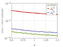
Figure 1: Error and error estimates of the approximated controllability Gramians for the Stokes system (4) after the first iteration of the reduced basis method.

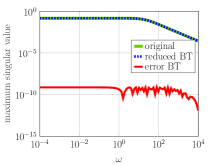
(a) Sigma plots of the original, reduced, and error transfer functions for the test parameter $\mu=1.28$.

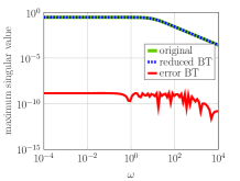
(b) Sigma plots of the original, reduced, and error transfer functions for the parameter $\mu=0.65$.

Figure 2: Results for the reduction of the Stokes system (4).

Our constant example matrices $E=I_{n},\,A,\,G,\,B_{1},\,C_{1}$ are created by the M-M.E.S.S. function $\mathtt{stokes\_FVM}$ and we choose the dimensions $n=3280,\,q=1681$, $m,\,p=1$, and the parameter set $\mathcal{D}=\left[\frac{1}{2},\,\frac{3}{2}\right]$. The test parameter set $\mathcal{D}_{\mathrm{Test}}$ consists of ten equidistant points within $\mathcal{D}$, i. e., $\mathcal{D}_{\mathrm{Test}}=\left\{\frac{1}{2}+\frac{1}{9}\cdot k\;\big{|}\;k=0,\,\ldots,\,9\right\}$. The matrices $B_{2}$ and $C_{2}$ are zero matrices. The reduced basis method from Section 4 produces bases of dimensions $24$ for both projected continuous-time Lyapunov equations. This basis generation is done in the offline phase, which takes $2.7\cdot 10^{3}$ seconds for this example. For the first iteration of the reduced basis method corresponding to the proper controllability Lyapunov equation, we evaluate the errors and their estimates from equation (28) and (29). They are presented in Figure 1, where the error is evaluated by

$$\textrm{error}\approx{\big{\|}\mathbf{P}_{\mathrm{p}}^{\mathrm{acc}}(\mu)-\mathbf{Z}(\mu)\mathbf{Z}(\mu)^{\mathrm{H}}\big{\|}}_{\mathrm{F}},$$

where $\mathbf{P}_{\mathrm{p}}^{\mathrm{acc}}(\mu)$ denotes an accurate approximation of the exact solution $\mathbf{P}_{\mathrm{p}}(\mu)$. For evaluating the error, the Lyapunov equations are also solved with the residual tolerance $10^{-15}$ to obtain an accurate estimate of the exact solution. After the first iteration step, we obtain an error that is already smaller than the tolerance $\mathrm{tol}=10^{-4}$. Additionally, we see that the error estimator $\Delta_{\mathbf{V}}^{(2)}$ provides an almost sharp bound of the actual error while $\Delta_{\mathbf{V}}^{(1)}$ leads to more conservative error bounds.

After we have determined the bases, we approximate the proper controllability and observability Gramians to apply balanced truncation in the online phase for two different parameters $\mu=1.28$ and $\mu=0.65$ where the first parameter is the eighth entry from the test parameter set $\mathcal{D}_{\mathrm{Test}}$. The reduced systems for both parameters are of dimension $r=10$ and consist only of differential states. This online phases last for $3.7\cdot 10^{-2}$ and $1.9\cdot 10^{-2}$ seconds, respectively, for this example. Figures 2a and 2b depict the transfer functions of the full and the reduced systems and the corresponding errors. We observe that the error is smaller than $10^{-8}$ for all $\omega$ in $[10^{-4},\,10^{4}]$. Additionally, in Figures 3a and 3b, we show the output $y(t)$ of the full system and the output $y_{\mathrm{R}}(t)$ of the reduced system for an input $u(t)=-2-\sin(t)$, $t\in[0,\,10]$, and the initial condition is given as $\mathbf{z}(0)=0$. We also depict the error ${\|y(t)-y_{\mathrm{R}}(t)\|}_{2}$ which is smaller than $10^{-8}$ in the entire time range. Hence, we can observe that the system behavior is well-approximated by the reduced system.

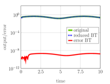
(a) Output plots of the original and reduced system and the corresponding error for the test parameter $\mu=1.28$.

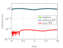
(b) Output plots of the original and reduced system and the corresponding error for the parameter $\mu=0.65$.

Figure 3: Output and output error of the original and reduced Stokes system (4)

Now, to demonstrate that the methods presented in this paper are also suitable for systems with an improper transfer function, we modify the system in such a way that the matrices $B_{2}$ and $C_{2}$ are chosen to be $B_{2}=\begin{bmatrix}0&\dots&0&1\end{bmatrix}^{\mathrm{T}}$ and $C_{2}=\begin{bmatrix}1&0&\dots&0&1\end{bmatrix}.$ That way, we obtain more complex restrictions for $G^{\mathrm{T}}x(t)$ and also evaluate the pressure described by $\lambda(t)$ to generate an output $y(t)$. We additionally assume that the external force represented by the input function $B_{1}(\mu)u(t)$ varies its magnitude depending on the viscosity of the system so that the input matrix $B_{1}(\mu)=(1+\mu)\cdot B_{1}$ is parameter-dependent, and hence, the polynomial part of the transfer function is parameter-dependent as well.

Again, in the offline phase, we execute the reduced basis method to generate bases that approximate the proper controllability and observability spaces (i. e., the image space of the corresponding proper Gramians) of this system. This phase takes $9.3\cdot 10^{3}$ seconds for this example. In Figure 4a and 4b, the errors and error estimations in the two stages of the reduced basis method corresponding to the proper controllability space are shown. For evaluating the error, the Lyapunov equations are also solved with the residual tolerance $10^{-15}$ to obtain an accurate estimate of the exact solution. We can observe that after the first iteration step, we obtain an error that is significantly larger than the tolerance $10^{-4}$ as shown in Figure 4a. Additionally, we see that the error estimator $\Delta_{\mathbf{V}}^{(2)}$ provides an almost sharp bound of the actual error while $\Delta_{\mathbf{V}}^{(1)}$ leads to more conservative error bounds. The second iteration of the reduced basis method and the corresponding errors are depicted in Figure 4b. In this case, the error as well as the estimators are smaller than the tolerance $\mathrm{tol}=10^{-4}$. The final basis projection space dimensions for the projected continuous-time Lyapunov equations are $48$ and $54$.

The next step is to use the bases to generate approximations of the system Gramians and to apply balanced truncation, which leads to a reduced system of dimension $25$ where we obtain $23$ differential states and $2$ algebraic ones for both parameters $\mu=1.28$ and $\mu=0.65$. The online phase lasts for $3.2$ and $3.1$ seconds if we use balanced truncation via the improper Gramians to reduce the improper system components and $2.4$ seconds for both parameters if we extract the polynomial part of the transfer function. However, in this example, the parameter dependency does not have a low-rank structure. Thus, for the determination of the polynomial part, it is necessary to solve one linear system of equations of full order in the online phase for each parameter of interest. Explicit formulas of the improper Gramians are also described in [55]. For a fixed parameter, also an explicit formula

$$\mathbf{S}_{\mathrm{i}}^{\mathrm{T}}\mathbf{A}\mathbf{R}_{\mathrm{i}}=\begin{bmatrix}B_{11}&C_{2}(G^{\mathrm{T}}G)^{-1}B_{2}\\ C_{2}(G^{\mathrm{T}}G)^{-1}B_{2}&0\end{bmatrix}$$ (39)

is provided with

$$B_{11}:=C_{1}G(G^{\mathrm{T}}G)^{-1}B_{2}+C_{2}(G^{\mathrm{T}}G)^{-1}G^{\mathrm{T}}B_{12},\qquad B_{12}:=B_{1}-AG(G^{\mathrm{T}}G)^{-1}B_{2},$$

compare with (14). This formula replaces the computation of the low-rank factors of the improper Gramians in the online phase. In our setting, (39) can be evaluated efficiently since all involved matrices can be precomputed and then appropriately scaled with $\mu$ in the parametric setting.

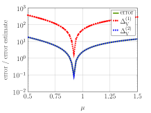
(a) First step of the reduced basis method.

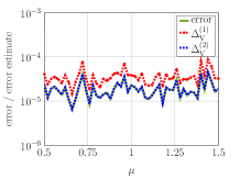
(b) Second step of the reduced basis method.

Figure 4: Error and error estimates of the approximated Gramians for the Stokes system (4) with improper parts.

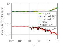
(a) Sigma plots of the original, reduced, and error transfer functions for the test parameter $\mu=1.28$.

(b) Sigma plots of the original, reduced, and error transfer functions for the parameter $\mu=0.65$.

Figure 5: Results for the reduction of the Stokes system (4) with improper parts.

We demonstrate the quality of the reduced systems by evaluating the error of the transfer functions. In the following, we denote the reduced system (error system) with an algebraic part generated by balanced truncation as reduced BT (error BT) and the reduced system (error system) with an algebraic part obtained by approximating the polynomial part of the transfer function as reduced TF (error TF). We show the sigma plot of the original and reduced transfer function as well as the error for two parameters. The first parameter, depicted in Figure 5a, is $\mu=1.28\in\mathcal{D}_{\mathrm{Test}}$ that is an element from the test parameter set and hence we already know that the error estimators $\Delta_{1/2}(\mu)$ are smaller than the tolerance and the proper controllability space is well-approximated. The second parameter is $\mu=0.65\in\mathcal{D}$, and the corresponding results are shown in Figure 5b. The polynomial part of the transfer function is clearly observable since it does not tend to zero for growing values of $\omega$. We observe that for both parameters, the error is smaller than $10^{-5}$ in the entire frequency band $[10^{-4},\,10^{6}]$ and that the parameter chosen from the test parameter set does not lead to significantly better approximations than an arbitrarily chosen parameter from the parameter set $\mathcal{D}$. This allows the conclusion that the basis $\mathbf{V}_{\mathrm{glob}}$ approximates the proper controllability space well — for all parameters in $\mathcal{D}$. Additionally, we can observe that both procedures to approximate the improper part of the system lead to satisfactory results.

Finally, to illustrate that the output $y$ is well approximated by the reduced output $y_{\mathrm{R}}$, in Figure 6a and 6b we evaluate the norms of the output error ${\|y(t)-y_{\mathrm{R}}(t)\|}_{2}$ for $t\in[0,\,100]$ for the test parameter $\mu=1.28$ and the parameter $\mu=0.65$. We choose the input function $u(t)=5-5\cdot\mathrm{cos}(t)$ and the initial condition $\mathbf{z}(0)=\begin{bmatrix}x(0)\\ \lambda(0)\end{bmatrix}=0$, in such a way that the consistency conditions are satisfied. We obtain an output error that is smaller than $10^{-5}$ for all $t\in[0,\,100]$ for both evaluated parameters. Again, we observe that both approximations of the algebraic part of the system lead to results of similar quality.

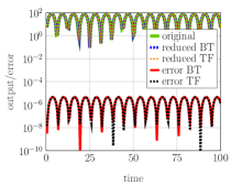
(a) Output plots of the original and reduced system and the corresponding error for the test parameter $\mu=1.28$.

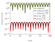
(b) Output plots of the original and reduced system and the corresponding error for the parameter $\mu=0.65$.

Figure 6: Output and output error of the original and reduced Stokes system (4) with improper parts

5.2 Problem 2: Mechanical system

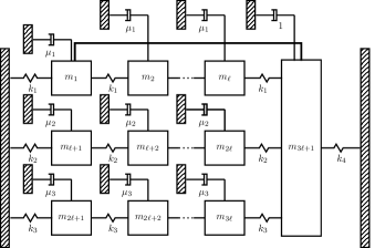
Figure 7: Constrained mass-damper-spring system including three chains of masses that are connected by the mass $m_{3\ell+1}$.

As an example for system (5), we consider a constrained mass-spring-damper system which is depicted in Figure 7 and which is similar to the one considered in [61]. The matrices are generated using the function triplechain_MSD from the M-M.E.S.S.-2.2. toolbox, see [46] where the mass matrix $M$ is built as

$$M=\begin{bmatrix}M_{1}&&&\\ &M_{2}&&\\ &&M_{3}&\\ &&&m_{0}\\ \end{bmatrix},\qquad M_{i}=m_{i}\cdot I_{\ell}\in\mathbb{R}^{\ell,\ell},\quad i=1,\,2,\,3$$

for $m_{1}=m_{2}=m_{3}=m_{0}=1$. The stiffness matrix is built as

$$K=\begin{bmatrix}K_{11}&&&\kappa_{1}\\ &K_{22}&&\kappa_{2}\\ &&K_{33}&\kappa_{3}\\ \kappa_{1}^{\mathrm{T}}&\kappa_{2}^{\mathrm{T}}&\kappa_{3}^{\mathrm{T}}&k_{1}+k_{2}+k_{3}+k_{0}\end{bmatrix},\quad K_{ii}=k_{i}\begin{bmatrix}2&-1&&&\\ -1&2&-1&&\\ &\ddots&\ddots&\ddots&\\ &&-1&2&-1\\ &&&-1&2\end{bmatrix}\in\mathbb{R}^{\ell,\ell},$$

with $\kappa_{i}=\begin{bmatrix}0&\dots&0&k_{i}\end{bmatrix}^{\mathrm{T}}$ and $k_{1}=k_{2}=k_{3}=k_{0}=1$. We set $\ell=200$ so that the dimension of $M$ and $K$ is $n=601$ and the matrix $G\in\mathbb{R}^{n,1}$ is a zero matrix except for the entries $G_{1,1}=1$ and $G_{n,1}=-1$. Hence, the first and the last mass are additionally connected by a rigid structure, as shown in Figure 7. Hence, the first-order system is of dimension $2n+2=1204$ after applying the transformation presented in Subsubsection 4.2.2. The input matrix $B_{x}\in\mathbb{R}^{n,1}$ is chosen as a zero matrix with one nonzero entry $(B_{x})_{450,1}=1.$ The output matrix $C_{x}\in\mathbb{R}^{1,n}$ is given by $C_{x}=B_{x}^{\mathrm{T}}$.

These systems occur in the field of damping optimization, see [16, 59, 61, 60], where the damping matrix $D\in\mathbb{R}^{n,n}$ consists of an internal damping $D_{\mathrm{int}}$ and some external dampers that need to be optimized. In our example, we choose Rayleigh damping as a model for the internal damping, i. e., $D_{\mathrm{int}}=\eta M+\rho K$, where we set $\eta=0.01$ and $\rho=0.02$. To describe the external damping, we assume that every mass is connected to a grounded damper, where the masses $m_{1},\,\ldots,\,m_{\ell}$ are connected by dampers with viscosity $\mu_{1}$, the masses $m_{\ell+1},\,\ldots,\,m_{2\ell}$ by dampers with viscosity $\mu_{2}$ and the masses $m_{2\ell+1},\,\ldots,\,m_{3\ell}$ by dampers with viscosity $\mu_{3}$ as depicted in Figure 7. The mass $m_{3\ell+1}$ is connected to a grounded damper with fixed viscosity $1$. The external dampers can be described by the matrices

$$F_{1}=\begin{bmatrix}I_{\ell}&\\ &0_{2\ell+1,2\ell+1}\end{bmatrix},\quad F_{2}=\begin{bmatrix}0_{\ell,\ell}&&\\ &I_{\ell}&\\ &&0_{\ell+1,\ell+1}\end{bmatrix},\quad F_{3}=\begin{bmatrix}0_{2\ell,2\ell}&&\\ &I_{\ell}&\\ &&0\end{bmatrix},\quad F_{4}=\begin{bmatrix}0_{3{\ell},3\ell}&\\ &1\end{bmatrix},$$

where $0_{n_{1},n_{2}}$ denotes the zero matrix in $\mathbb{R}^{n_{1},n_{2}}$. Therefore, the overall damping matrix can then be constructed as

$$D(\mu) :=D_{\mathrm{int}}+\mu_{1}F_{1}+\mu_{2}F_{2}+\mu_{3}F_{3}+F_{4},$$

where $\mu=[\mu_{1},\mu_{2},\mu_{3}]\in\mathcal{D}$ are the viscosities of the dampers, which are optimized and thus variable in our model. This model leads to a differential-algebraic system of index 3. We generate the index-2 surrogate system as shown in Subsubsection 4.2.2 using the value $\gamma(\mu)=\frac{1}{2}\gamma^{*}(\mu)$ from (36).

We consider two parameter settings. In the first one, the system is damped more strongly, and in the second one more weakly. The latter setting is used to illustrate that the slightly damped system is more difficult to approximate by projection spaces of small dimensions, which poses a challenge from the numerical point of view. For both parameter settings, the reduced models are obtained by truncating all state variables corresponding to proper Hankel singular values with $\sigma_{\mathrm{p},k}/\sigma_{\mathrm{p},1}<10^{-8}$.

5.2.1 Setting 1: Stronger external damping

We consider the parameter set $\mathcal{D}=[0.1,1]^{3}$ and choose the test parameter set $\mathcal{D}_{\mathrm{Test}}$ to consist of 50 randomly selected parameter triples from $\mathcal{D}$. Therefore, we use the $\mathtt{rand}$ operator from MATLAB so that the $k$-th test parameter is equal to $\mu=0.1+0.9\cdot\mathtt{rand}(3,1)$ with fixed seed.

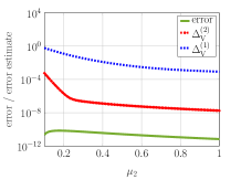
Figure 8: Error and error estimates of the approximated controllability Gramians of the mechanical system (5) with stronger external damping and $\mu_{1}=0.25$, $\mu_{3}=0.35$ after the first iteration of the reduced basis method.

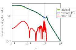
(a) Sigma plots of the original, reduced, and error transfer functions for the test parameter $\mu=\begin{bmatrix}0.2622,\,0.1175,\,0.5169\end{bmatrix}$.

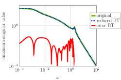
(b) Sigma plots of the original, reduced, and error transfer functions for the parameter $\mu=\begin{bmatrix}0.15,\,0.15,\,0.5\end{bmatrix}$.

Figure 9: Results for the reduction of the mechanical system (5) with stronger external damping.

In the offline phase, the approximation of the controllability and observability spaces takes $1.4\cdot 10^{4}$ seconds for this example. For the proper controllability space, we evaluate the errors and the error estimates that are depicted in Figure 8 for the first iteration of the reduced basis method. For evaluating the error, the Lyapunov equations (9) are also solved by computing the projection matrices $\boldsymbol{\Pi}_{\mathrm{l}}(\mu)$ and $\boldsymbol{\Pi}_{\mathrm{r}}(\mu)$ explicitly and solving the corresponding Lyapunov equation. Therefore, we fix the parameters $\mu_{1}=0.25$ and $\mu_{3}=0.35$ and show the errors for the varying second parameter $\mu_{2}\in[0.1,1]$. After the first iteration and for a basis of dimension $219$, the maximal error estimate $\Delta_{\mathbf{V}}^{(2)}$ is equal to $9.48\cdot 10^{-5}$. Hence, the basis approximates the proper controllability space sufficiently well. Again, we see that the error estimator $\Delta_{\mathbf{V}}^{(2)}$ approximates the error $\mathfrak{E}(\cdot)$ better than the estimation by $\Delta_{\mathbf{V}}^{(1)}$, which massively overestimates the error. Hence, we only use the error estimator $\Delta_{\mathbf{V}}^{(2)}$ to determine the basis quality.

We need two iterations of the reduced basis method to determine the respective observability subspace of dimension of $304$. Hence, we have to solve Lyapunov equations of dimensions $219$ and $304$ in the online phase to compute the Gramian approximations. We apply the online phase for the parameters $\mu=\begin{bmatrix}0.2622,\,0.1175,\,0.5169\end{bmatrix}\in\mathcal{D}_{\mathrm{Test}}\subset\mathcal{D}$ (which is rounded to 4 digits here) and $\mu=\begin{bmatrix}0.15,\,0.15,\,0.5\end{bmatrix}\in\mathcal{D}$. We obtain the two respective reduced systems of dimension $75$ and $63$, where all states are differential ones. The online phases take $6.4\cdot 10^{-1}$ and $1.3\cdot 10^{-1}$ seconds, respectively, for this example.

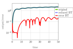
(a) Output plots of the original and reduced system and the corresponding error for the test parameter $\mu=\begin{bmatrix}0.2622,\,0.1175,\,0.5169\end{bmatrix}$.

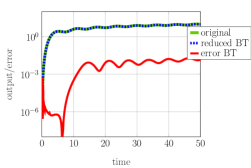
(b) Output plots of the original and reduced system and the corresponding error for the parameter $\mu=\begin{bmatrix}0.15,\,0.15,\,0.5\end{bmatrix}$.

Figure 10: Output and output error of the original and reduced system (5) with stronger external damping.

In Figure 9, we depict the original, the reduced, and the error transfer function. Additionally, we evaluate the outputs of the original and the reduced system $y$ and $y_{\mathrm{R}}$. The results are shown in Figure 10, where we observe the norm of the output error ${\|y(t)-y_{\mathrm{R}}(t)\|}_{2}$ for $t\in[0,50]$. We choose the input function $u(t)=1-1\cdot\cos(t)$ and the initial condition $\mathbf{z}(0)=\begin{bmatrix}x(0)\\ \lambda(0)\end{bmatrix}=0$, so that the consistency conditions are satisfied. We observe that the output error is smaller than $10^{-2}$ for all $t\in[0,\,50]$. Note that for damping optimization examples, the proper controllability and observability spaces are often hard to approximate by spaces of small dimensions, see [58, 11]. Hence, the tolerances are chosen rather large for this kind of example to achieve satisfying results.

5.2.2 Setting 2: Weaker external damping

Now, we consider a parameter set with viscosities of small magnitudes, that is $\mathcal{D}=[0.01,0.1]^{3}$. The test-parameter set $\mathcal{D}_{\mathrm{Test}}$ consists of 50 randomly selected parameters from $\mathcal{D}$. To generate the test parameters, we again use the $\mathtt{rand}$ operator from MATLAB so that the $k$-th parameter is equal to $\mu=0.01+0.09\cdot\mathtt{rand}(3,1)$ with fixed seed.

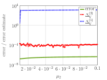
Figure 11: Error and error estimates of the approximated observability Gramians of the mechanical system (5) with weaker external damping and $\mu_{1}=0.025$, $\mu_{3}=0.035$ after the first iteration of the reduced basis method.

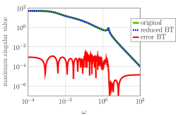
(a) Sigma plots of the original, reduced, and error transfer functions for the test parameter $\mu=\begin{bmatrix}0.0886,\,0.0972,\,0.0882\end{bmatrix}$.

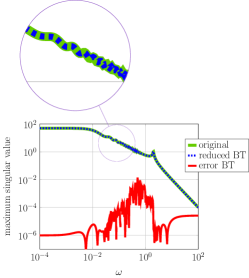
(b) Sigma plots of the original, reduced, and error transfer functions for the parameter $\mu=\begin{bmatrix}0.01,\,0.02,\,0.01\end{bmatrix}$. The magnifying glass illustrates that the reduced-order model captures the strong oscillations in the sigma plot very well.

Figure 12: Results for the reduction of the mechanical system (5) with weaker external damping.

First, we apply the offline phase of the reduced basis method that takes $6.9\cdot 10^{3}$ seconds. When computing the proper controllability space, two iterations are needed to generate a subspace of dimension $449$ that leads to error estimates $\Delta_{\mathbf{V}}^{(2)}(\mu)$ that are at most $5.6\cdot 10^{-4}$. For the proper observability space, the errors and the error estimates are illustrated in Figure 11 within the first iteration of the reduced basis method with fixed parameters $\mu_{1}=0.025$ and $\mu_{3}=0.035$ and varying $\mu_{2}\in[0.01,0.1]$. For evaluating the error, the Lyapunov equations (10) are also solved by computing the projection matrices $\boldsymbol{\Pi}_{\mathrm{l}}(\mu)$ and $\boldsymbol{\Pi}_{\mathrm{r}}(\mu)$ explicitly and solving the corresponding Lyapunov equation. After the first iteration, we determine a basis of dimension $223$ for which the maximal error estimate $\Delta_{\mathbf{V}}^{(2)}$ is equal to $5.8\cdot 10^{-4}$, and hence, sufficient accuracy is achieved. As for the first parameter setting, the error estimator $\Delta_{\mathbf{V}}^{(2)}$ approximates the error $\mathfrak{E}(\cdot)$ better than the estimation by $\Delta_{\mathbf{V}}^{(1)}$. Hence, we use the error estimator $\Delta_{\mathbf{V}}^{(2)}$ within the reduced basis method. We apply the online phase for the parameters $\mu=\begin{bmatrix}0.0886,\,0.0972,\,0.0882\end{bmatrix}\in\mathcal{D}_{\mathrm{Test}}\subset\mathcal{D}$ (which is rounded to 4 digits) and $\mu=\begin{bmatrix}0.01,\,0.02,\,0.01\end{bmatrix}\in\mathcal{D}$ to derive a reduced-order model of dimension $78$ for the first parameter and the reduced dimension $178$ for the second one. The online phases need $2.21$ and $2.04$ seconds, respectively.

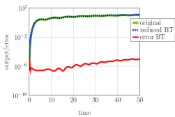
(a) Output plots of the original and reduced system and the corresponding error for the test parameter $\mu=\begin{bmatrix}0.089,\,0.097,\,0.088\end{bmatrix}$.

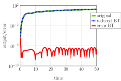
(b) Output plots of the original and reduced system and the corresponding error for the parameter $\mu=\begin{bmatrix}0.01,\,0.02,\,0.01\end{bmatrix}$.

Figure 13: Output and output error of the original and reduced mechanical system (5) with weaker external damping.

Figure 12 depicts the original, the reduced, and the error transfer function. Additionally, we evaluate the norm of the output error ${\|y(t)-y_{\mathrm{R}}(t)\|}_{2}$ for $t\in[0,50]$ in Figure 13, where the input function $u(t)=1-1\cdot\mathrm{cos}(t)$ and the initial condition $\mathbf{z}(0)=\begin{bmatrix}x(0)\\ \lambda(0)\end{bmatrix}=0$ are chosen in such a way that the consistency conditions are satisfied. We observe that the output error is smaller than $10^{-4}$ for all $t\in[0,\,50]$.

6 Conclusions

This paper has addressed the model reduction of parameter-dependent differential-algebraic systems by balanced truncation. To apply the balancing procedure we have utilized specific projectors to eliminate the algebraic constraints. This has enabled us to compute the necessary Gramians efficiently by solving projected Lyapunov equations.

To handle the parameter-dependency, we have applied the reduced basis method, which is split into the offline phase and the online phase. In the offline phase, we have computed the basis of the subspace which approximates the solution space of the parametric Lyapunov equations. To assess the quality of this subspace we have derived two error estimators. Afterwards, in the online phase, we have solved a reduced Lyapunov equation to obtain an approximation of the Gramian for a parameter value of interest efficiently. Therefore, a balanced truncation for this parameter value can also be carried out fast.

This method has been illustrated by numerical examples of index two and three. In particular, we were often able to reduce the associated Lyapunov equations to very small dimensions. We have evaluated our error estimators, where the second one can often estimate the error almost exactly.

Code availability

The code and data that has been used to generate the numerical results of this work are freely available under the DOI 10.5281/zenodo.10040792 under the 3-clause BSD license and is authored by Jennifer Przybilla.

CRediT author statement

Jennifer Przybilla: Methodology, Software, Data Curation, Writing — Original Draft, Writing — Review & Editing, Visualization; Matthias Voigt: Conceptualization, Writing — Original Draft, Writing — Review & Editing, Supervision.

References

• [1] G. Alì, N. Banagaaya, W. H. A. Schilders, and C. Tischendorf. Index-aware model order reduction for differential-algebraic equations. Math. Comput. Model. Dyn. Syst., 20(4):345–373, 2014. doi:10.1080/13873954.2013.829501.
• [2] A. C. Antoulas. Approximation of Large-Scale Dynamical Systems, volume 6 of Adv. Des. Control. SIAM Publications, Philadelphia, PA, 2005. doi:10.1137/1.9780898718713.
• [3] A. C. Antoulas, I. V. Gosea, and M. Heinkenschloss. Data-driven model reduction for a class of semi-explicit DAEs using the Loewner framework. In T. Reis and A. Ilchmann, editors, Progress in Differential-Algebraic Equations II, Differ.-Algebr. Equ. Forum, pages 185–210. Springer, 2020. doi:10.1007/978-3-030-53905-4_7.
• [4] N. Banagaaya. Index-Aware Model Order Reduction Methods for DAEs. Proefschrift, Technische Universiteit Eindhoven, The Netherlands, 2014. doi:10.6100/IR780937.
• [5] N. Banagaaya, G. Ali, and W. H. A. Schilders. Index-aware Model Order Reduction Methods, volume 2 of Atlantis Stud. Sci. Comput. Electromagn. Atlantis Press, 2016.
• [6] R. H. Bartels and G. W. Stewart. Solution of the matrix equation ${AX}+{XB}={C}$: Algorithm 432. Comm. ACM, 15:820–826, 1972. doi:10.1145/361573.361582.
• [7] U. Baur, C. A. Beattie, P. Benner, and S. Gugercin. Interpolatory projection methods for parameterized model reduction. SIAM J. Sci. Comput., 33(5):2489–2518, 2011. doi:10.1137/090776925.
• [8] U. Baur, P. Benner, and L. Feng. Model order reduction for linear and nonlinear systems: A system-theoretic perspective. Arch. Comput. Methods Eng., 21(4):331–358, 2014. doi:10.1007/s11831-014-9111-2.
• [9] C. A. Beattie, S. Gugercin, and V. Mehrmann. Structure-preserving interpolatory model reduction for port-Hamiltonian differential-algebraic systems. In C. Beattie, P. Benner, M. Embree, S. Gugercin, and S. Lefteriu, editors, Realization and Model Reduction of Dynamical Systems, pages 235–254. Springer, Cham, 2022. doi:10.1007/978-3-030-95157-3_13.
• [10] P. Benner, S. Gugercin, and K. Willcox. A survey of projection-based model reduction methods for parametric dynamical systems. SIAM Rev., 57(4):483–531, 2015. doi:10.1137/130932715.
• [11] P. Benner, P. Kürschner, Z. Tomljanović, and N. Truhar. Semi-active damping optimization of vibrational systems using the parametric dominant pole algorithm. ZAMM Z. Angew. Math. Mech., 96(5):604–619, 2016. doi:10.1002/zamm.201400158.
• [12] P. Benner, M. Ohlberger, A. Cohen, and K. Willcox, editors. Model Reduction and Approximation: Theory and Algorithms. Comput. Sci. Eng. SIAM, Philadelphia, PA, 2017. doi:10.1137/1.9781611974829.
• [13] P. Benner, J. Saak, and M. M. Uddin. Balancing based model reduction for structured index-2 unstable descriptor systems with application to flow control. Numer. Algebra Control Optim., 6(1):1–20, 2016. doi:10.3934/naco.2016.6.1.
• [14] P. Benner and A. Schneider. Balanced truncation for descriptor systems with many terminals. Max Planck Institute Magdeburg Preprints MPIMD/13-17, 2013. Available at https://csc.mpi-magdeburg.mpg.de/preprints/2013/MPIMD13-17.pdf.
• [15] P. Benner and T. Stykel. Model order reduction for differential-algebraic equations: A survey. In A. Ilchmann and T. Reis, editors, Surveys in Differential-Algebraic Equations IV, Differ.-Algebr. Equ. Forum, pages 107–160. Springer, Cham, 2017. doi:10.1007/978-3-319-46618-7_3.
• [16] P. Benner, Z. Tomljanović, and N. Truhar. Dimension reduction for damping optimization in linear vibrating systems. ZAMM Z. Angew. Math. Mech., 91(3):179–191, 2011. doi:10.1002/zamm.201000077.
• [17] T. Berger, A. Ilchmann, and S. Trenn. The quasi-Weierstraß form for regular matrix pencils. Linear Algebra Appl., 436:4052–4069, 2012. doi:10.1016/j.laa.2009.12.036.
• [18] K. E. Brenan, S. L. Campbell, and L. R. Petzold. Numerical Solution of Initial-Value Problems in Differential-Algebraic Equations. SIAM, Philadelphia, PA, 1995. doi:10.1137/1.9781611971224.
• [19] S. L. Campbell. Singular Systems of Differential Equations, volume 40 of Res. Notes Math. Pitman Advanced Publishing Program, London, 1980. doi:10.1002/nme.1620150916.
• [20] S. L. Campbell, C. D. Meyer, and N. J. Rose. Applications of the Drazin inverse to linear systems of differential equations with singular constant coefficients. Comput. Math. Appl., 31(3):411–425, 1976. doi:10.1137/0131035.
• [21] V. Druskin and V. Simoncini. Adaptive rational Krylov subspaces for large-scale dynamical systems. Systems Control Lett., 60(8):546–560, 2011. doi:10.1016/j.sysconle.2011.04.013.
• [22] R. Eid, R. Castañé-Selga, H. Panzer, T. Wolf, and B. Lohmann. Stability-preserving parametric model reduction by matrix interpolation. Math. Comput. Model. Dyn. Syst., 17(4):319–335, 2011. doi:10.1080/13873954.2011.547671.
• [23] G. Flagg, C. Beattie, and S. Gugercin. Convergence of the iterative rational Krylov algorithm. Systems Control Lett., 61(6):688–691, 2012. doi:10.1016/j.sysconle.2012.03.005.
• [24] M. Geuss, H. Panzer, and B. Lohmann. On parametric model order reduction by matrix interpolation. In Proceedings of the 12th European Control Conference, pages 3433–3438, Strasbourg, France, 2013. doi:10.23919/ECC.2013.6669829.
• [25] K. Glover. All optimal Hankel-norm approximations of linear multivariable systems and their L norms. Internat. J. Control, 39:1115–1193, 1984. doi:10.1080/00207178408933239.
• [26] I. V. Gosea, C. Poussot-Vassal, and A. C. Antoulas. Data-driven modeling and control of large-scale dynamical systems in the Loewner framework: methodology and applications. In E. Zuazua and E. Trelat, editors, Numerical Control: Part A, Handb. Numer. Anal. Elsevier, 2021.
• [27] I. V. Gosea, Q. Zhang, and A. C. Antoulas. Preserving the DAE structure in the Loewner model reduction and identification framework. Adv. Comput. Math., 46:3, 2020. doi:10.1007/s10444-020-09752-8.
• [28] S. Gugercin, A. C. Antoulas, and C. Beattie. $\mathcal{H}_{2}$ model reduction for large-scale linear dynamical systems. SIAM J. Matrix Anal. Appl., 30(2):609–638, 2008. doi:10.1137/060666123.
• [29] S. Gugercin, T. Stykel, and S. Wyatt. Model reduction of descriptor systems by interpolatory projection methods. SIAM J. Sci. Comput., 35(5):B1010–B1033, 2013. doi:10.1137/130906635.
• [30] S. J. Hammarling. Numerical solution of the stable, non-negative definite Lyapunov equation. IMA J. Numer. Anal., 2:303–323, 1982. doi:10.1093/imanum/2.3.303.
• [31] M. Heinkenschloss, D. C. Sorensen, and K. Sun. Balanced truncation model reduction for a class of descriptor systems with application to the Oseen equations. SIAM J. Sci. Comput., 30(2):1038–1063, 2008. doi:10.1137/070681910.
• [32] J. S. Hesthaven, G. Rozza, and B. Stamm. Certified Reduced Basis Methods for Parametrized Partial Differential Equations. SpringerBriefs Math. Springer, Cham, 2016. doi:10.1007/978-3-319-22470-1.
• [33] R. A. Horn and C. R. Johnson. Topics in Matrix Analysis. Cambridge University Press, Cambridge, 1991. doi:10.1017/CBO9780511840371.
• [34] P. Kunkel and V. Mehrmann. Differential-Algebraic Equations: Analysis and Numerical Solution. Textbooks in Mathematics. EMS Publishing House, Zürich, Switzerland, 2006. ISBN: 3037190175.
• [35] P. Kürschner. Efficient Low-Rank Solution of Large-Scale Matrix Equations. Dissertation, Otto-von-Guericke-Universität, Magdeburg, Germany, April 2016. URL: http://hdl.handle.net/11858/00-001M-0000-0029-CE18-2.
• [36] P. Lancaster and M. Tismenetsky. The Theory of Matrices. Academic Press, Orlando, 2nd edition, 1985. ISBN: 9780124355606.
• [37] R. März. Canonical projectors for linear differential algebraic equations. Comput. Math. Appl., 31(4/5):121–135, 1996. doi:10.1016/0898-1221(95)00224-3.
• [38] A. Massoudi, M. R. Opmeer, and T. Reis. The ADI method for bounded real and positive real Lur’e equations. Numer. Math., 135(2):431–458, 2017. doi:10.1007/s00211-016-0805-2.
• [39] A. J. Mayo and A. C. Antoulas. A framework for the solution of the generalized realization problem. Linear Algebra Appl., 425(2–3):634–662, 2007. doi:10.1016/j.laa.2007.03.008.
• [40] V. Mehrmann and T. Stykel. Balanced truncation model reduction for large-scale systems in descriptor form. In P. Benner, V. Mehrmann, and D. C. Sorensen, editors, Dimension Reduction of Large-Scale Systems, volume 45 of Lect. Notes Comput. Sci. Eng., pages 83–115. Springer, Berlin/Heidelberg, 2005. doi:10.1007/3-540-27909-1_3.
• [41] B. C. Moore. Principal component analysis in linear systems: controllability, observability, and model reduction. IEEE Trans. Automat. Control, AC–26(1):17–32, 1981. doi:10.1109/TAC.1981.1102568.
• [42] H. Panzer, T. Wolf, and B. Lohmann. A strictly dissipative state space representation of second order systems. at-Automatisierungstechnik, 60(7):392–397, 2012. doi:10.1524/auto.2012.1015.
• [43] T. Penzl. A cyclic low rank Smith method for large sparse Lyapunov equations. SIAM J. Sci. Comput., 21(4):1401–1418, 2000. doi:10.1137/S1064827598347666.
• [44] R. Pulch, A. Narayan, and T. Stykel. Sensitivity analysis of random linear differential–algebraic equations using system norms. J. Comput. Appl. Math., 397:113666, 2021. doi:10.1016/j.cam.2021.113666.
• [45] A. Quarteroni, A. Manzoni, and F. Negri. Reduced Basis Methods for Partial Differential Equations, volume 92 of La Matematica per il 3+2. Springer International Publishing, 2016. ISBN: 978-3-319-15430-5.
• [46] J. Saak, M. Köhler, and P. Benner. M-M.E.S.S.-2.2 – The Matrix Equations Sparse Solvers library, February 2022. doi:10.5281/zenodo.5938237.
• [47] J. Saak and M. Voigt. Model reduction of constrained mechanical systems in M-M.E.S.S. IFAC-PapersOnLine, 51(2):661–666, 2018. 9th Vienna International Conference on Mathematical Modelling, Vienna, 2018. doi:10.1016/j.ifacol.2018.03.112.
• [48] A. Schmidt, D. Wittwar, and B. Haasdonk. Rigorous and effective a-posteriori error bounds for nonlinear problems – Application to RB methods. Adv. Comput. Math., 46:32, 2020. doi:10.1007/s10444-020-09741-x.
• [49] P. Schwerdtner, T. Moser, V. Mehrmann, and M. Voigt. Optimization-based model order reduction of port-Hamiltonian descriptor systems. Systems Control Lett., 2023. To appear.
• [50] V. Simoncini and V. Druskin. Convergence analysis of projection methods for the numerical solution of large Lyapunov equations. SIAM J. Numer. Anal., 47(2):828–843, 2009. doi:10.1137/070699378.
• [51] N. T. Son, P.-Y. Gousenbourger, E Massart, and T. Stykel. Balanced truncation for parametric linear systems using interpolation of Gramians: a comparison of algebraic and geometric approaches. In P. Benner, T. Breiten, H. Faßbender, M. Hinze, T. Stykel, and R. Zimmermann, editors, Model Reduction of Complex Dynamical Systems, volume 171 of Internat. Ser. Numer. Math., pages 31–51. Birkhäuser, Cham, 2021. doi:10.1007/978-3-030-72983-7_2.
• [52] N. T. Son and T. Stykel. Solving parameter-dependent Lyapunov equations using the reduced basis method with application to parametric model order reduction. SIAM J. Matrix Anal. Appl., 38(2):478–504, 2017. doi:10.1137/15M1027097.
• [53] D. C. Sorenson and Y. Zhou. Bounds on eigenvalue decay rates and sensitivity of solutions to Lyapunov equations. CAAM Technical Reports TR02-07, Rice University, 2002. Available at https://repository.rice.edu/items/7d1381b1-adc7-4282-8486-430784cef15c.
• [54] T. Stykel. Gramian-based model reduction for descriptor systems. Math. Control Signals Systems, 16(4):297–319, 2004. doi:10.1007/s00498-004-0141-4.
• [55] T. Stykel. Balanced truncation model reduction for semidiscretized Stokes equation. Linear Algebra Appl., 415(2–3):262–289, 2006. doi:10.1016/j.laa.2004.01.015.
• [56] T. Stykel. Low-rank iterative methods for projected generalized Lyapunov equations. Electron. Trans. Numer. Anal., 30:187–202, 2008. URL: http://etna.mcs.kent.edu/vol.30.2008/pp187-202.dir/pp187-202.pdf.
• [57] M. S. Tombs and I. Postlethwaite. Truncated balanced realization of a stable non-minimal state-space system. Internat. J. Control, 46(4):1319–1330, 1987. doi:10.1080/00207178708933971.
• [58] Z. Tomljanović, C. Beattie, and S. Gugercin. Damping optimization of parameter dependent mechanical systems by rational interpolation. Adv. Comput. Math., 44(6):1797–1820, 2018. doi:10.1007/s10444-018-9605-9.
• [59] N. Truhar, Z. Tomljanović, and M. Puvača. Approximation of damped quadratic eigenvalue problem by dimension reduction. Appl. Math. Comput., 347:40–53, 2019. doi:10.1016/j.amc.2018.10.047.
• [60] N. Truhar and K. Veselić. An efficient method for estimating the optimal dampers’ viscosity for linear vibrating systems using Lyapunov equation. SIAM J. Matrix Anal. Appl., 31(1):18–39, 2009. doi:10.1137/070683052.
• [61] M. Ugrica. Approximation of Quadratic Eigenvalue Problem and Application to Damping Optimization. Doctoral thesis, University of Zagreb, Faculty of Science, Zagreb, Croatia, 2020. https://urn.nsk.hr/urn:nbn:hr:217:106554.
• [62] B. Wang and F. Zhang. Some inequalities for the eigenvalues of the product of positive semidefinite Hermitian matrices. Linear Algebra Appl., 160:113–118, 1992. doi:10.1016/0024-3795(92)90442-D.
• [63] K. Zhou, J. C. Doyle, and K. Glover. Robust and Optimal Control. Prentice-Hall, Upper Saddle River, NJ, 1996. ISBN: 0-13-456567-3.