Transition from metal to higher-order topological insulator driven by random flux

Abstract

Random flux is commonly believed to be incapable of driving full metal-insulator transitions in non-interacting systems. Here we show that random flux can after all induce a full metal-band insulator transition in the two-dimensional Su-Schrieffer-Heeger model. Remarkably, we find that the resulting insulator can be an extrinsic higher-order topological insulator with zero-energy corner modes in proper regimes, rather than a conventional Anderson insulator. Employing both level statistics and finite-size scaling analysis, we characterize the metal-band insulator transition and numerically extract its critical exponent as $\nu=2.48\pm 0.08$. To reveal the physical mechanism underlying the transition, we present an effective band structure picture based on the random flux averaged Green’s function.

Introduction.—Disorder, being present in most physical systems, constitutes a broad field of physics research. As one of its most salient effects, random potential disorder can induce metal-Anderson insulator transitions in various systems Anderson (1958); Evers and Mirlin (2008); Sanchez-Palencia and Lewenstein (2010); Schwartz et al. (2007); Chabé et al. (2008), prominently topological phase transitions Li et al. (2009); Groth et al. (2009); Jiang et al. (2009); Guo et al. (2010), as recently observed in cold-atom and photonic systems Meier et al. (2018); Stützer et al. (2018). Random flux is another generic type of disorder that has been widely investigated in two-dimensional (2D) electron systems Cerovski (2001); Furusaki (1999); Aronov et al. (1994); Taras-Semchuk and Efetov (2000); Sheng and Weng (1995); Liu et al. (1995); Zhang and Arovas (1994); Gade (1993); Sugiyama and Nagaosa (1993); Avishai et al. (1993); Lee and Fisher (1981); AnJ and Lin (2001); Foster and Ludwig (2008). Yet, it is believed that random flux is unable to drive a system with chiral symmetry from metal to Anderson insulator if the Fermi energy locates precisely at zero: instead it localizes all states except the ones at the band centre Cerovski (2001); Furusaki (1999). Moreover, the interplay between random flux and topology has barely been explored.

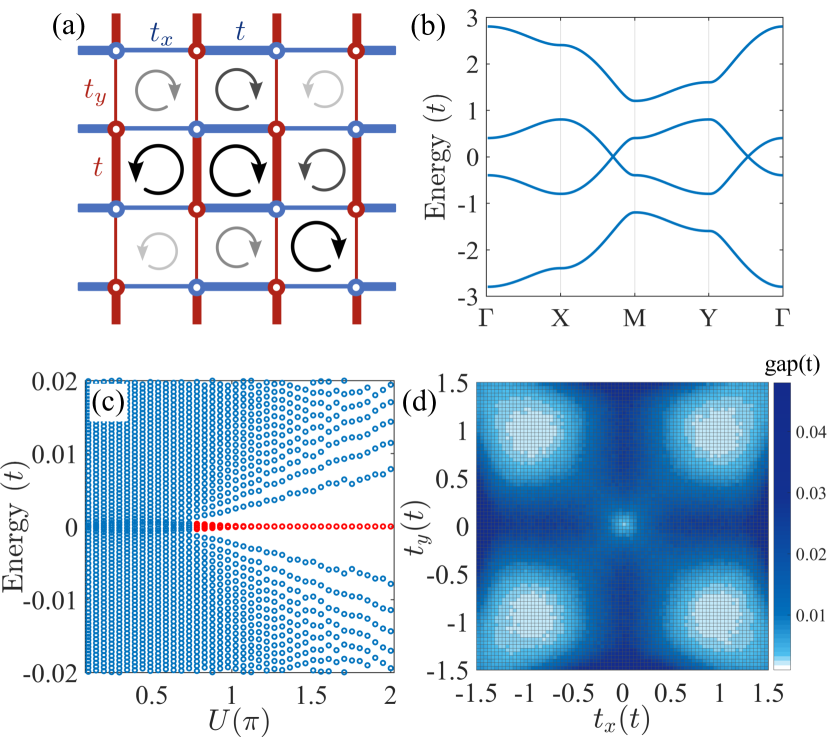
Figure 1: (a) Schematic of the 2D SSH model with random flux. Blue(red) thick and thin bonds mark dimerized hopping amplitudes in $x(y)$-direction. The round arrow (with different sizes and opacity) in each plaquette indicates the random flux. (b) Energy spectrum of the model without random flux for $(t_{x},t_{y})=(0.2t,0.6t)$. (c) Disorder-averaged spectrum as a function of $U$ for $(t_{x},t_{y})=(0.2t,0.6t)$. For large $U$, the system acquires a bulk gap that protects four zero-energy modes (red). (d) Density plot of the directly disorder-averaged gap as a function of $t_{x}$ and $t_{y}$ at $U=2\pi$. The dimension of the system is $L\equiv L_{x}=L_{y}=30$ with open (periodic) boundaries in (c) [(d)]. Here, 200 random-flux configurations are considered.

In this work, we discover a random-flux driven metal-band insulator transition. To this end, we add random flux to the 2D Su-Schrieffer-Heeger (SSH) lattice model [Fig. 1(a)] which has attracted broad interest recently Liu and Wakabayashi (2017); Benalcazar et al. (2017a, b). In the absence of random flux, this model has been realized in different physical platforms Schindler et al. (2018a); Imhof et al. (2018); Serra-Garcia et al. (2018); Xie et al. (2019); Qi et al. (2020); Peterson et al. (2018); Ni et al. (2019); Chen et al. (2019), and sparked the rapidly developing field of higher-order topological phases Langbehn et al. (2017); Song et al. (2017); Schindler et al. (2018b); Ezawa (2018); Geier et al. (2018); Trifunovic et al. (2019); Imhof et al. (2018); Serra-Garcia et al. (2018); Xie et al. (2019); Qi et al. (2020); Peterson et al. (2018); Ni et al. (2019); Chen et al. (2019); Liu et al. (2019); Luo and Zhang (2019); Ghorashi et al. (2020); Wang et al. (2020); Kudo et al. (2019); Volpez et al. (2019); Wang et al. (2019); Yan et al. (2018); Zhang et al. (2020a); Li et al. (2020); Chen et al. (2020); Yang et al. (2021); Zhang et al. (2020b); Li et al. (2020b). Importantly, the existence of a metallic phase in the clean 2D SSH model and its rich topological properties due to non-trivial inner degrees of freedom provide a promising playground for revisiting the issue of random-flux driven transitions in the context of topological band structures.

Remarkably, we find that the spectrum of the system acquires a finite bulk gap in a broad parameter range when exceeding a critical strength of random flux [Figs. 1(c) and 1(d)], thus transforming from a metallic phase to a band insulator. This metal-band insulator transition is confirmed and carefully analyzed by employing energy level statistics and finite-size scaling theory. The corresponding critical exponent is estimated to be $\nu=2.48\pm 0.08$. Interestingly, we find that the band insulator induced by random flux can be an extrinsic higher-order topological insulator (HOTI) by calculating the topological index $q_{xy}$ and identifying the corresponding boundary signatures. Furthermore, with an effective band structure picture based on the flux-averaged Green’s function, we show that the metal-band insulator transition can be attributed to the emergence of strongly momentum-dependent flux-induced terms that have a non-trivial matrix structure in the effective Hamiltonian. By contrast, such an interplay of random flux and internal degrees of freedom in the unit cell is absent in the conventional random-flux model.

2D SSH lattice with random flux.—As visualized in Fig. 1(a), the 2D SSH lattice model features dimerized hopping amplitudes along both $x$- and $y$-directions Liu and Wakabayashi (2017). In the absence of disorder, it can be described by the Hamiltonian

$$H_{0}({\bf k})= (t_{x}+t\cos k_{x})\tau_{1}\sigma_{0}-t\sin k_{x}\tau_{2}\sigma_{3}$$

$$+(t_{y}+t\cos k_{y})\tau_{1}\sigma_{1}-t\sin k_{y}\tau_{1}\sigma_{2},$$ (1)

where $\tau$ and $\sigma$ are Pauli matrices for different degrees of freedom within a unit cell; ${\bf k}=(k_{x},k_{y})$ is the 2D wave-vector; $t$ and $t_{x}$$(t_{y}$) denote the two staggered hopping strengths in $x$$(y)$-direction. For simplicity, we put the lattice constant to unity and assume $t>0$. Note that $k_{x}$ and $k_{y}$ are decoupled in Eq. (1). The total Hamiltonian can be recast as the sum of two SSH models along $x$- and $y$-directions, respectively, i.e., $H_{0}(\mathbf{k})=H_{x}(k_{x})+H_{y}(k_{y})$. The matrices $\tau_{1}\sigma_{0}$ and $\tau_{2}\sigma_{3}$ contained in $H_{x}(k_{x})$ anticommute with each other. The same holds for the matrices $\tau_{1}\sigma_{1}$ and $\tau_{1}\sigma_{2}$ contained in $H_{y}(k_{y})$. However, the two blocks commute with each other, i.e., $[H_{x}(k_{x}),H_{y}(k_{y})]=0$. As a consequence, the four energy bands of Eq. (1) are given by $E_{\eta}^{\pm}=\pm[\epsilon_{x}(k_{x})+(-1)^{\eta}\epsilon_{y}(k_{y})]$ with $\epsilon_{\alpha}(k_{\alpha})=\sqrt{t_{\alpha}^{2}+2t_{\alpha}t\cos k_{\alpha}+t^{2}}$, $\alpha\in\{x,y\}$ and $\eta\in\{1,2\}$. When $||t_{x}|-|t_{y}||<2t$, the system is in a metallic phase at low energies [Fig. 1(b)]. The model has $C_{2v}$ group symmetry in general ($t_{x}\neq t_{y}$). Moreover, it respects chiral symmetry $\gamma_{5}H_{0}({\bf k})\gamma_{5}^{-1}=-H_{0}({\bf k})$ with the chiral operator $\gamma_{5}=\tau_{3}\sigma_{0}$. In the clean case, the constituting 1D blocks along $x$- and $y$-directions are topologically nontrivial when $|t_{x}|<t$ and $|t_{y}|<t$, respectively. This property can be identified by symmetry indicators based on the symmetry representations at high-symmetry points in Brillouin zone that are described in Refs. Benalcazar et al. (2019); Krutoff et al. (2017); Po et al. (2017); Li (2). We note that there may be corner-localized bound states in the bulk continuum, while their stability needs to be protected by $C_{4v}$ symmetry Benalcazar and Cerjan (2020); Cerjan et al. (2020) which corresponds to $t_{x}=t_{y}$ in Eq. (1).

We now add random flux to the model such that each plaquette encloses a flux that has random values drawn from a uniformly distributed interval $[-U/2,U/2]$, as illustrated in Fig. 1(a). Here, $U$ is the strength of random flux within the range of $[0,2\pi]$, in units of the magnetic flux quantum $\Phi_{0}=hc/e$ Note (1). The random flux generates random Peierls phases in the hopping matrix elements. Thus, time reversal symmetry is broken. However, chiral symmetry is still preserved and plays a crucial role in the metal-insulator transition as we elaborate below. Note that when each plaquette encloses a $\pi$ flux uniformly, the system is deformed to the Benalcazar-Bernevig-Hughes (BBH) model Benalcazar et al. (2017a, b)

Metal-band insulator transition driven by random flux.—Next, we demonstrate the existence of random-flux driven metal-band insulator transitions in the 2D SSH model by employing level statistics Wigner (1951); Dyson (1962). In the presence of chiral symmetry, the model falls into the chiral unitary universality class, i.e., AIII in AZ classification Altland et al. (1997). The insulating and metallic phases can be distinguished by inverse participation ratio (IPR) Li et al. (2017); Roy et al. (2021); Padhan et al. (2022) and level spacing ratio (LSR) Yang et al. (2021); Oganesyan and Huse (2007). The IPR is defined by the eigenstates $\phi_{n}({\bf R},\zeta)$ of the system as

$$I_{n}= \sum_{{\bf R}}\sum_{\zeta=1}^{4}|\phi_{n}({\bf R},\zeta)|^{4},$$ (2)

where the sums run over all unit cells labeled by ${\bf R}$ and the inner degrees of freedom $\zeta$ within a unit cell. The subscript $n$ stands for the $n$-th state with the corresponding eigenenergy $E_{n}$ listed in ascending order. The LSR is defined in terms of the spectrum as Oganesyan and Huse (2007)

$$r_{n}=\frac{\mathrm{min}(s_{n},s_{n-1})}{\mathrm{max}(s_{n},s_{n-1})},$$ (3)

where $s_{n}\equiv E_{n+1}-E_{n}$ is the difference between two adjacent energy levels. Both the averaged IPR $\langle I\rangle$ and LSR $\langle r\rangle$ take different values in the metallic and insulating limits, thus providing important tools to characterize metal-insulator transitions.

We show below that the level statistics smoothly cross over between the two limits as the random flux drives the system from a metallic to an insulating phase. Due to the presence of chiral symmetry, the eigenenergies of the system come in pairs ($\pm E_{n}$). For illustration, we take $t_{x}=0.2t$ and $t_{y}=0.6t$ and consider an energy window containing $N_{E}$ energy levels around $E=0$. Figure 2(a) displays $\langle I\rangle$ as a function of $U$. Clearly, $\langle I\rangle$ increases monotonically from nearly zero in the small $U$ limit to finite values for large $U.$ This indicates that the system transits from a metallic (with vanishing $\langle I\rangle$) to an insulating phase (with finite $\langle I\rangle$). Concomitant with the transformation of $\langle I\rangle$, we also observe that $\langle r\rangle$ decreases smoothly from a universal value $0.6$ at small $U$ ($\simeq 0$) to another universal value $0.386$ at large $U$ ($\simeq 2\pi$), as shown in Fig. 2(b). For sufficiently large $L$, the numerical values approach the universal constants in both limits of $U$. These results agree with those obtained for the uncorrelated Poisson ensemble in the insulating phase ($\langle r\rangle_{\mathrm{ins}}\approx 0.386$) Oganesyan and Huse (2007) and the unitary ensemble in the metallic phase ($\langle r\rangle_{\mathrm{met}}\approx 0.6$) Atas et al. (2013), respectively.

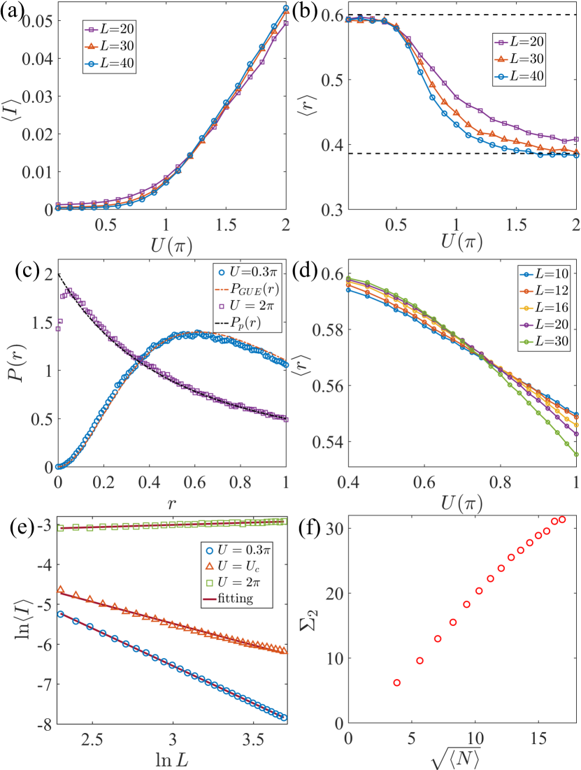
Figure 2: (a) Averaged IPR $\langle I\rangle$ as a function of $U$ for $L=20$, $30$, and $40$, respectively. (b) Averaged LSR $\langle r\rangle$ as a function of $U$ for $L=20$, $30$, and $40$, respectively. (c) Distribution of LSR $P(r)$ in different limits. (d) Averaged LSR $\langle r\rangle$ near the critical point as a function of $U$ for various $L$. (e) Scaling behavior of IPR in the metallic (blue) and insulating (green) phases, and at the critical point $U_{c}\approx 0.75\pi$ (red). (f) Number variance $\Sigma_{2}$ as a function of $\sqrt{\langle N\rangle}$ at the critical point. We consider $N_{E}=16$ and 4000 random-flux configurations in (a,b,c,e). The parameters $t_{x}=0.2t$, $t_{y}=0.6t$ and periodic boundary conditions are chosen for all plots.

To better illustrate the transition, we analyze the probability distribution $P(r)$ of LSR Not (b). As shown in Fig. 2(c), $P(r)$ also exhibits universal but different forms in the small and large $U$ regimes, respectively Not (b). For small $U$, we find that $P(r)$ can be well described by the distribution function of the Gaussian unitary ensemble (GUE) $P_{\text{GUE}}(r)=\frac{81\sqrt{3}}{2\pi}\frac{(r+r^{2})^{2}}{(1+r+r^{2})^{4}}$ Atas et al. (2013). This finding supports that the system is in a metallic phase. For large $U$, $P(r)$ instead resembles the uncorrelated Poisson distribution $P_{\text{p}}(r)=\frac{2}{(1+r)^{2}}$, which again hallmarks an insulating phase Oganesyan and Huse (2007). These results provide direct evidence that the system undergoes a metal-insulator transition by increasing $U$. This metal-insulator transition is generic for parameters fulling $||t_{x}|-|t_{y}||<2t$, $t_{x}\neq t$, and $t_{x}\neq t$ Note (3). It is, however, absent for $t_{x}=t_{y}=t$ which corresponds to the conventional random-flux model Li (2). We note that the band gap opening by random flux [see Fig. 1(c)] may modify the statistical behavior of low energy states close to the band center.

Critical exponent.—Critical exponents are keys for characterizing continuous phase transitions. To identify the critical exponent $\nu$ and critical random-flux strength $U_{c}$, we perform a finite-size scaling analysis of the averaged LSR $\langle r\rangle$ Laumann et al. (2014); Luitz et al. (2015); Luo et al. (2021). According to the single-parameter scaling theory, $\langle r\rangle$ shows a size-independent value at $U=U_{c}$. Concentrating around the zero energy, we fix the energy window to capture $10\%$ of the eigenvalues and choose the number of random-flux configurations in such a way that the total eigenvalue number reaches $5\times 10^{7}$. As shown in Fig. 2(d), $\langle r\rangle$ increases as the system size $L$ grows before the transition whereas it decreases as $L$ grows after the transition. The scaling argument near $U_{c}$ states that $\langle r\rangle$ can be described by a universal function of the form $F(f_{1}(u)L^{1/\nu},f_{2}(u)L^{-y})$ characterized by $\nu$, where $u\equiv(U-U_{c})/U_{c},$ and $y$ is an auxiliary exponent; $f_{1}(u)L^{1/\nu}$ and $f_{2}(u)L^{-y}$ stand for relevant and irrelevant length-scale corrections, respectively Slevin and Ohtsuki (2014); Luo et al. (2021). Close to $U_{c}$, we expand $f_{\eta}(u)=\sum_{j=0}^{m_{\eta}}a_{j}^{\eta}u^{j}$ with $\eta\in\{1,2\}$. Thus, $\nu$ and $U_{c}$ can be identified by fitting the Taylor expansion of the function $F$ near the critical point Slevin and Ohtsuki (2014); Luo et al. (2021). Thereby, we identify the critical exponent of the random-flux driven metal-band insulator transition as $\nu=2.48\pm 0.08$. This critical exponent is close to that of integer quantum Hall transitions with $\nu\approx 2.59$ Slevin and Ohtsuki (2009). In contrast to $\nu$ exponent , the critical strength $U_{c}$ depends explicitly on the parameters $t_{x}$ and $t_{y}$. For the parameters considered in Fig. 2(d), we find $U_{c}\approx 0.75\pi$, in accordance with the gap opening [Fig. 1(c)].

Fractal dimension and spectral rigidity.—At the critical point, the wavefunctions of the system show multifractality due to strong fluctuations Evers and Mirlin (2000); Mirlin and Evers (2000). The multifractality gives rise to one of the fractal dimensions $d_{2}$ defined through the scaling behavior $\langle I\rangle\propto L^{-d_{2}}$. Figure 2(e) displays $\ln\langle I\rangle$ as a function of $\ln L$ at small, large, and critical values of $U$, respectively. At the critical point $U=U_{c}$ (triangles), we can extract $d_{2}=1.085\pm 0.034$. At $U=0.3\pi$ (circles) and $U=2\pi$ (squares), we obtain $d_{2}=1.880\pm 0.006$ and $0.119\pm 0.008$, which are close to the values of an ideal metal (corresponding to $d_{2}=2$) and an insulator (corresponding to $d_{2}=0$), respectively.

The spectral rigidity is also related to the wavefunction multifractality. It is defined as the level number variance $\Sigma_{2}\equiv\langle N^{2}\rangle-\langle N\rangle^{2}$ in an energy window, where $\langle N\rangle$ is the disorder-averaged number of energy levels within this window. For conventional Anderson transitions, $\Sigma_{2}\propto\langle N\rangle$ at the critical point when the energy window is sufficiently large. The ratio $\chi\equiv\Sigma_{2}/\langle N\rangle$ defines the compressibility of the spectrum. It is conjectured that $d_{2}$ is related to $\chi$ by the relation $\chi=(2-d_{2})/4$ in 2D Chalker et al. (1996a, b). However, our scaling law follows instead $\Sigma_{2}\propto\sqrt{\langle N\rangle}$ [Fig. 2(f)], resembling the complex Ginibre ensemble Ginibre (1965). This behavior may be due to the fact that the random flux gives a complex matrix ensemble. Thus, $\chi$ goes to zero in the large $N$ limit, and the aforementioned conjecture fails in our system.

Effective band structure picture for the metal-band insulator transition.—To reveal the underlying mechanism, we average the Green’s function over many random-flux configurations, so as to effectively restore lattice translation-invariance and derive the self-energy $\Sigma({\bf k})$ due to the random flux Li (2); Note (6). We find that $\Sigma({\bf k})$ not only modifies the coefficient functions of the matrices in the original Hamiltonian [c.f. Eq. (1)] but also introduces additional terms associated with new matrices $\tau_{1}\sigma_{3}$ and $\tau_{2}\sigma_{0}$ (that also appear in the BBH model). This feature can be understood in terms of higher-order scattering processes induced by random flux. It is intimately related to the interplay between the internal degrees of freedom of the model and the random flux that couples directly to momentum in the system. Consequently, $\Sigma({\bf k})$ decisively depends on momentum. These observations indicate that the effective Hamiltonian $H_{\mathrm{eff}}({\bf k})\equiv H_{0}({\bf k})+\Sigma({\bf k})$ for the system with random flux can be regarded as a mixture of the 2D SSH and BBH models. Remarkably, a band gap for strong $U$ can be directly revealed by the effective band structure of $H_{\mathrm{eff}}({\bf k})$ Li (2). The critical value $U_{c}$ of random flux strength obtained here is consistent with the numerical result in Fig. 1(c). In this sense, the random flux generates a band insulator by opening an effective gap in the bulk after the transition.

Extrinsic HOTI induced by random flux.—Now, we show that in the parameter regime $|t_{x}|<t$ and $|t_{y}|<t$, the band insulator induced by random flux can be an extrinsic HOTI  Geier et al. (2018); Trifunovic et al. (2019). For concreteness, we consider $U=2\pi$. In this case, the system is an insulator with a finite energy gap, unless $|t_{x}|=|t_{y}|=t$, c.f. Fig. 1(d) Note (4). Note that the disorder-averaged flux on each plaquette is zero. The defined electric quadrupole moment $q_{xy}$ can provide a topological index to characterize the extrinsic HOTI Benalcazar et al. (2017a, b); Kang et al. (2019); Wheeler et al. (2019); Roy (2019). In the phase diagram shown in Fig. 3(a), which is similar to that of BBH model, we observe a nontrivial region (blue) with a half quantized $q_{xy}=1/2$. In the outer region (white), the system is a trivial insulator with $q_{xy}=0$. This implies that the random-flux driven higher-order topological phases can be continuously connected to that of the BBH model. The quantization of $q_{xy}$ is protected by chiral symmetry Li et al. (2020). Accordingly, a nontrivial $q_{xy}$ indicates the emergence of zero-energy modes at the corners of the system. This is confirmed numerically in Figs. 1(c) and 3(c) where four zero-energy modes clearly emerge in the nontrivial phase whereas they disappear in the trivial phase. Furthermore, we calculate the local charge density at half-filling [Fig. 3(b)]. Summing the charge density over each quadrant including a single corner, we find that the total charge takes fractional values $\pm 1/2$ as long as $L$ is large enough. These fractional corner charges provide another hallmark of the HOTI.

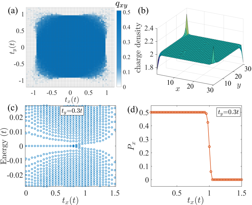
Figure 3: (a) Phase diagram of $q_{xy}$ against $t_{x}$ and $t_{y}$. The dimension of the system is $L=30$ with 30 random-flux configurations. (b) Electron charge density in the extrinsic HOTI phase at half-filling. (c) Disorder-averaged energy spectrum as a function of $t_{x}$ for $t_{y}=0.3t$ under open boundary conditions. (d) Disorder-averaged edge polarization $P_{x}$ as a function of $t_{x}$ for $t_{y}=0.3t$. $U=2\pi$ for all plots.

For a fixed strong $U$, the system transits between an extrinsic HOTI and a trivial insulator by changing $t_{x}$ or $t_{y}$. Due to its extrinsic nature, the topological phase transitions take place at the boundaries instead of the bulk of the system. To elucidate this phase transition, we calculate the effective Hamiltonian $H_{\mathrm{edge}}$ for edges in the presence of random flux via a recursive Green’s function method Peng et al. (2017); Note (5). We see the edge spectrum close and reopen around phase boundary. Alternatively, the transition can also be shown from the edge polarization of $H_{\mathrm{edge}}$ Benalcazar et al. (2017b); Resta (1998). For illustration, we consider the edge along $x$-direction and present the disorder-averaged polarization $P_{x}$ as a function of $t_{x}$ in Fig. 3(d). Near $t_{x}=t$, $P_{x}$ changes suddenly from $1/2$ to 0, indicating a topological phase transition. The results for edges along $y$-direction can be obtained similarly. We note that the system is nontrivial only if both edge Hamiltonians along $x$- and $y$-directions are nontrivial.

Discussion and conclusions.— Note that the metal-band insulator transition driven by random flux is found to also occur in the topologically trivial regime Li (2), which indicates its generality. Clearly, the random flux with zero mean is different from the case with a uniform flux, where the Hofstadter butterfly emerges Otaki and Fukui (2019); Zuo et al. (2021); Hofstadter (1976). In the limit of $t_{x}=t_{y}=t$, our system reduces to the conventional random-flux model. In this limit, we recover the well established result that the bulk states at the band center stay delocalized and no metal-insulator transition occurs Li (2). We emphasize that the random-flux driven metal-band insulator transition is distinctively different from related work in interacting systems AnJ and Lin (2001); Foster and Ludwig (2008) where the competition between (random) flux and electron-electron interaction is responsible for an interaction driven phase transition.

The 2D SSH model can be realized in different platforms such as metamaterials Serra-Garcia et al. (2018); Ni et al. (2019); Xie et al. (2019); Qi et al. (2020); Chen et al. (2019), microwave and electric circuits Peterson et al. (2018); Imhof et al. (2018); Dong et al. (2021); Zhang et al. (2021). In particular, the manipulation of effective magnetic fluxes has become experimentally accessible in sonic crystals and circuit simulators Lin et al. (2021); Li et al. (2021). Therefore, these materials may provide us with promising platforms to test our predictions by taking advantage of their high controllability.

In conclusion, based on the 2D SSH model we have revealed the first example of a metal-band insulator transition that is solely driven by random flux. We have analyzed this metal-band insulator transition by level statistics and finite-size scaling theory, and found the critical exponent as $\nu=2.48\pm 0.08$. It is shown that the emergent insulator can be an extrinsic HOTI by presenting its phase diagram and characteristic boundary signatures. We have further proposed an effective band structure picture to understand the metal-band insulator transition driven by random flux.

Supplemental material for “Transition from metal to higher-order topological insulator driven by random flux”

Appendix S1 Properties of the 2D SSH model

In this section, we present the band structure and phase diagram of the 2D Su-Schrieffer-Heeger (SSH) model in the clean limit. The Hamiltonian in momentum space is given by

$$H_{0}({\bf k})=(t_{x}+t\cos k_{x})\tau_{1}\sigma_{0}-t\sin k_{x}\tau_{2}\sigma_{3}+(t_{y}+t\cos k_{y})\tau_{1}\sigma_{1}-t\sin k_{y}\tau_{1}\sigma_{2},$$ (S1.1)

where $\tau$ and $\sigma$ are Pauli matrices for different degrees of freedom within a unit cell; ${\bf k}=\{k_{x},k_{y}\}$ is the 2D wavevector; $t$ and $t_{x}$ $(t_{y}$) denotes the two staggered hopping strengths along $x$ $(y)$ directions. We set the lattice constant to unity for simplicity. Note that $k_{x}$ and $k_{y}$ are decoupled in Eq. (S1.1). The total Hamiltonian can be recast as the sum of two SSH models along $x$ and $y$ directions, respectively, $H_{0}(\mathbf{k})=H_{x}(k_{x})+H_{y}(k_{y})$. Accordingly, the four matrix terms in Eq. (S1.1) can be divided into two groups $G_{1}=\{\tau_{1}\sigma_{0},\tau_{2}\sigma_{3}\}$ and $G_{2}=\{\tau_{1}\sigma_{1},\tau_{1}\sigma_{2}\}$. The matrices are anticommute within each group but are commute between the groups. Thus, the four energy bands of Eq. (S1.1) can be found analytically as

$$E_{\eta}^{\pm}=\pm[\epsilon_{x}(k_{x})+(-1)^{\eta}\epsilon_{y}(k_{y})],$$ (S1.2)

where $\epsilon_{\alpha}(k_{\alpha})=\sqrt{t_{\alpha}^{2}+2t_{\alpha}t\cos k_{\alpha}+t^{2}}$, $\alpha\in\{x,y\}$ and $\eta\in\{1,2\}$.

A Gapless phase with nodal lines

Due to chiral symmetry, the two bands touch each other at $E=0$, when

$$\sqrt{t_{x}^{2}+2t_{x}t\cos k_{x}+t^{2}}=\sqrt{t_{y}^{2}+2t_{y}t\cos k_{y}+t^{2}},$$ (S1.3)

which gives rise to nodal lines in the $k_{x}\text{-}k_{y}$ plane. These nodal lines are due to the independency of $H_{x}(k_{x})$ and $H_{y}(k_{y})$. Thus, they are not protected by any specific symmetries. The condition for a gapless phase is

$$|t_{x}^{2}-t_{y}^{2} |\leq 2|t_{y}t|+2|t_{x}t|,$$ (S1.4)

or more concisely,

$$||t_{x}|-|t_{y}||\leq 2|t|.$$ (S1.5)

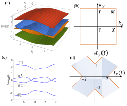
Figure S1: (a) Band structures with nodal lines for $t_{x}=0.1t$ and $t_{y}=0.3t$. (b) Brillouin zone with high symmetry points. (c) Band structure along the high symmetry lines for $t_{x}=0.1t$ and $t_{y}=0.3t$. (d) Gapless phase region (shadowed) in the ($t_{x},t_{y}$) parameter space.

B Symmetries

The 2D SSH model possesses a number of symmetries, as listed in Table 1.

Table 1: Symmetry properties of the 2D SSH model. Here, $K$ stands for the complex conjugation.

Symmetry	Operator	Operation
chiral	$\gamma_{5}=\tau_{3}\sigma_{0}$	$\gamma_{5}H_{0}({\bf k})\gamma_{5}^{-1}=-H_{0}({\bf k})$
time-reversal	$\mathcal{T}=\tau_{0}\sigma_{0}K$	$\mathcal{T}H_{0}({\bf k})\mathcal{T}^{-1}=H_{0}(-{\bf k})$
particle-hole	$\mathcal{P}=\tau_{3}\sigma_{0}K$	$\mathcal{P}H_{0}({\bf k})\mathcal{P}^{-1}=-H_{0}(-{\bf k})$
inversion	$\mathcal{I}=\tau_{0}\sigma_{1}$	$\mathcal{I}H_{0}({\bf k})\mathcal{I}^{-1}=H_{0}(-{\bf k})$
mirror $x$	$M_{x}=\tau_{1}\sigma_{0}$	$M_{x}H_{0}(k_{x},k_{y})M_{x}^{-1}=H_{0}(-k_{x},k_{y})$
mirror $y$	$M_{y}=\tau_{1}\sigma_{1}$	$M_{y}H_{0}(k_{x},k_{y})M_{y}^{-1}=H_{0}(k_{x},-k_{y})$
PT	$S=\tau_{0}\sigma_{1}K$	$SH_{0}({\bf k})S^{-1}=H_{0}({\bf k})$

In general, the 2D SSH model has $C_{2v}$ group symmetry, which includes mirror symmetries $M_{x}$ and $M_{y}$ with respect to the $x$ and $y$ axes, respectively, and $C_{2}$ rotation symmetry. The symmetry representation at the high symmetry points of the Brillouin zone witness the topological properties ((Benalcazar et al., 2019; Benalcazar and Cerjan, 2020)). The character table of the $C_{2v}$ group is listed in Table 2. There are only one-dimensional irreducible representations. At the high symmetry points, the wavefunctions form the basis of irreducible representations of the $C_{2v}$ group, as shown in Table 3. Since the Hamiltonian can be decoupled as $H_{0}(\mathbf{k})=H_{x}(k_{x})+H_{y}(k_{y})$, we can compare the representations at the $X$ ($Y$) point relative to the $\Gamma$ point to determine whether the system is topological or not along the $x$ ($y$) direction. For example, in the case 3 of Table 3, all the bands at the $X$ point have different representations relative to the $\Gamma$ point. Namely, the representation changes between $A_{(1,2)}$ $\leftrightarrow B_{(1,2)}$ when going from $X$ to $\Gamma$ points, implying a parity shift. Thus, the system is nontrivial along the $x$ direction. On the other hand, all the bands at the $Y$ point have the same representations compared to the $\Gamma$ point. Therefore, the system is trivial along the $y$ direction. Based on this method, we conclude that the system is nontrivial along $x$ ($y$) direction when $|t_{x}|<1$ ($|t_{y}|<1$). Otherwise, it is trivial. This classification is consistent with the spectrum of a ribbon along $x$ ($y$) direction, as shown in Fig. S2.

Table 2: Character table of the $C_{2v}$ group

	I	$C_{2}$	$M_{x}$	$M_{y}$
$A_{1}$	1	1	1	1
$A_{2}$	1	1	-1	-1
$B_{1}$	1	-1	1	-1
$B_{2}$	1	-1	-1	1

Table 3: Symmetry representations of the $C_{2v}$ group at the high symmetry points in the Brillouin zone. Irreducible representations $A_{1},A_{2},B_{1}$ and $B_{2}$ are all one dimensional.

	bands	$\Gamma$	$X$	$Y$
case 1: $|t_{x}|<1,|t_{y}|<1$	#1	$A_{2}$	$B_{1}$	$B_{2}$
	#2	$B_{1}$	$A_{2}$	$A_{1}$
	#3	$B_{2}$	$A_{1}$	$A_{2}$
	#4	$A_{1}$	$B_{2}$	$B_{1}$
case 2: $|t_{x}|>1,|t_{y}|>1$	#1	$A_{2}$	$A_{2}$	$A_{2}$
	#2	$B_{1}$	$B_{1}$	$B_{1}$
	#3	$B_{2}$	$B_{2}$	$B_{2}$
	#4	$A_{1}$	$A_{1}$	$A_{1}$
case 3: $|t_{x}|<1,|t_{y}|>1$	#1	$A_{2}$	$B_{1}$	$A_{2}$
	#2	$B_{1}$	$A_{2}$	$B_{1}$
	#3	$B_{2}$	$A_{1}$	$B_{2}$
	#4	$A_{1}$	$B_{2}$	$A_{1}$
case 4: $|t_{x}|>1,|t_{y}|<1$	#1	$A_{2}$	$A_{2}$	$B_{2}$
	#2	$B_{2}$	$B_{2}$	$A_{2}$
	#3	$B_{1}$	$B_{1}$	$A_{1}$
	#4	$A_{1}$	$A_{1}$	$B_{1}$

In the $C_{2v}$ group, there is no 2D irreducible representation. Consequently, the zero-energy modes stemming from nontrivial topology (for $|t_{x,y}|<1$) easily hybridize with degenerate bulk states. Thus, they are unstable. For the special case $t_{x}=t_{y}$, the system has $C_{4v}$ group symmetry. Because of the 2D irreducible representation of the $C_{4v}$ group together with chiral symmetry, the zero-energy modes are protected from the hybridization with the degenerate bulk states in this case (Benalcazar and Cerjan, 2020).

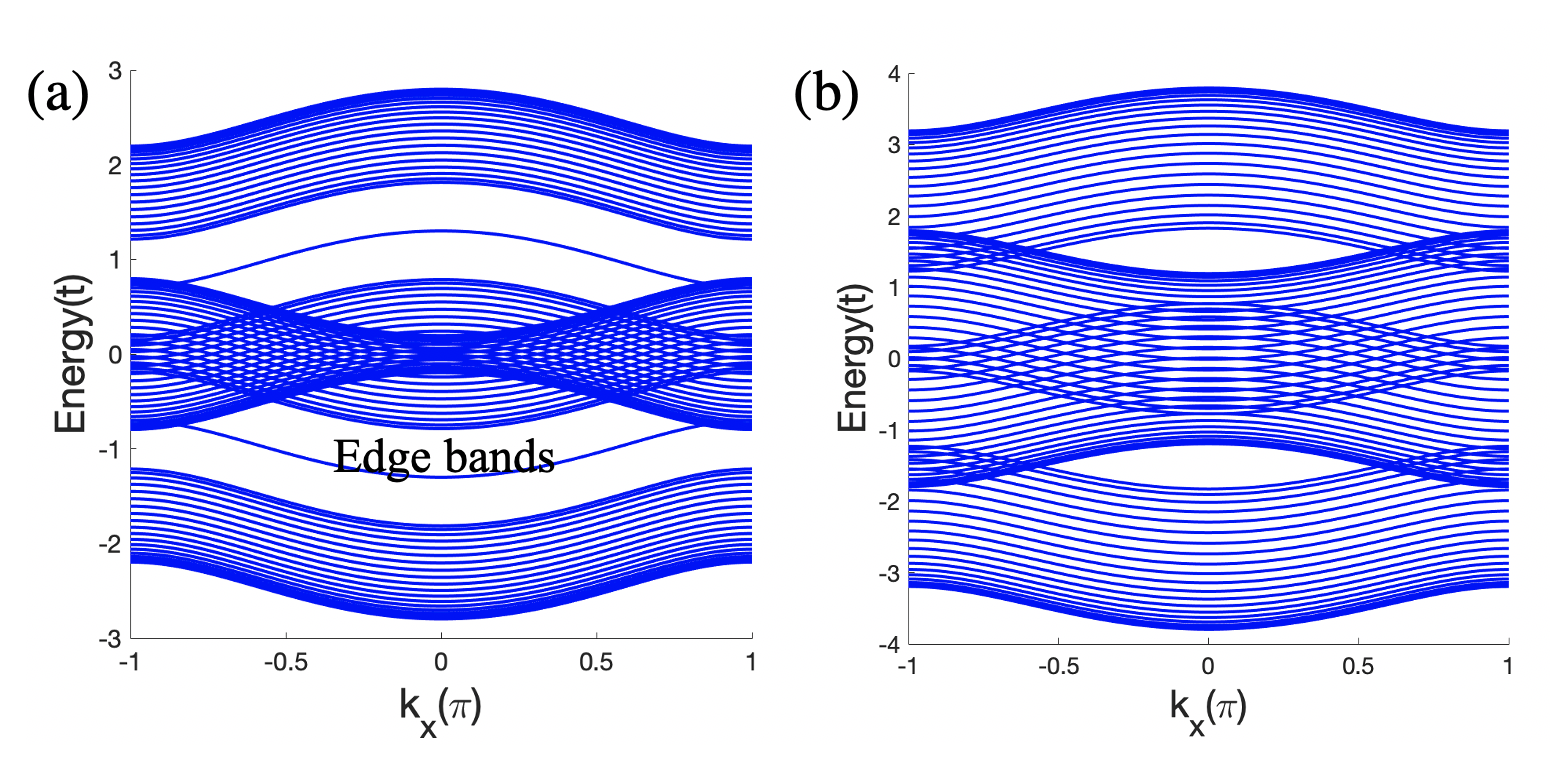
Figure S2: (a) Band structure in the $k_{x}$ direction of the model with open boundaries along the $y$ direction for $t_{x}=0.3t$ and $t_{y}=0.5t$. The system is nontrivial with edge bands (isolated lines) along the $y$ direction. (b) Band structure in the $k_{x}$ direction of the model with open boundaries along the $y$ direction for $t_{x}=0.3t$ and $t_{y}=1.5t$. The system is trivial without edge bands along $y$ direction.

Appendix S2 Metal-insulator transition in the trivial regime

In this section, we show that the metal-insulator transition by random flux also occurs in the topologically trivial regime (with $|t_{x(y)}|>t$) of the 2D SSH model. The results are displayed in Fig. S3. Clearly, the random flux opens a band gap beyond a critical random flux strength $U$, similar to the topological regime. However, there are no zero-energy corner modes in the insulating phase. Correspondingly in Fig. S3(b), the LSR is close to the value $0.6$ for small $U$ and approaches $0.386$ for large $U$. These results confirm the metal-insulator transition driven by the random flux in the topologically trivial regime.

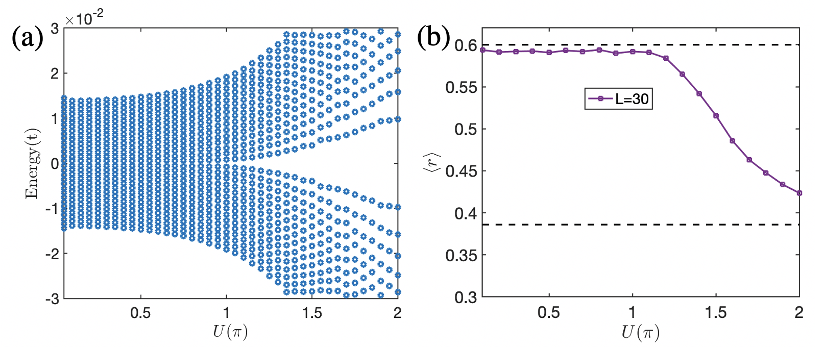
Figure S3: (a) Energy spectrum as a function of $U$ for $t_{x}=2t$ and $t_{y}=1.6t$. There are no degenerate zero-energy states in the insulating phase. 40 energy levels around zero energy are shown. (b) LSR as a function of $U$ near the band center for $t_{x}=2t$ and $t_{y}=1.6t$. We take $L=40$ ($30$) and $200(4000)$ disorder configurations in (a)[(b)]. $\langle r\rangle$ at $U=2\pi$ is still away from $0.386$ because the critical point $U_{c}$ is large and a finite size effect is significant for $L=40$ (30).

Appendix S3 Effective Hamiltonian and band structure

In this section, we derive and analyze the effective Hamiltonian $H_{\text{eff}}$ and energy spectrum of the system averaged over random flux configurations. For each random flux configuration, we can find the retarded Green’s function $G^{R}({\bf r},{\bf r}^{\prime};\omega)$ in the original basis of tight-binding model as

$$G^{R}({\bf r},{\bf r}^{\prime};\omega) =\langle{\bf r}|(\omega+i\eta-H_{\text{rand}})^{-1}|{\bf r}^{\prime}\rangle,$$ (S3.1)

where $\omega$ is frequency, $\eta$ is an infinitesimal positive number, and $H_{\text{rand}}$ is the lattice Hamiltonian with the random flux. We assume periodic boundary conditions in both $x$ and $y$ directions. Averaging over many random-flux configurations, translation invariance is effectively restored in both directions. Thus, the disorder-average Green’s function

$$G_{\mathrm{avg}}^{R}({\bf r}-{\bf r}^{\prime},\omega) =\langle G^{R}({\bf r},{\bf r}^{\prime};\omega)\rangle_{\mathrm{dis}},$$ (S3.2)

depends only on ${\bf r}-{\bf r}^{\prime}$. We perform Fourier transformation of the disorder-averaged Green’s function

$$G^{R}({\bf k},\omega) =\int d({\bf r}-{\bf r}^{\prime})G_{\mathrm{avg}}^{R}({\bf r}-{\bf r}^{\prime},\omega)e^{i{\bf k}\cdot({\bf r}-{\bf r}^{\prime})}.$$ (S3.3)

Without loss of generality, we replace ${\bf r}-{\bf r}^{\prime}$ by ${\bf r}$ and consider the discretization of ${\bf r}$ in the lattice model. Then, Eq. (S3.3) can be recast as

$$G^{R}({\bf k},\omega) =\sum_{{\bf r}}G_{\mathrm{avg}}^{R}({\bf r},\omega)e^{i{\bf k}\cdot{\bf r}}.$$ (S3.4)

This procedure allows us to derive the effective Hamiltonian as

$$H_{\mathrm{eff}}({\bf k})=-[G^{R}({\bf k},\omega=0)]^{-1}.$$ (S3.5)

The corresponding energy band structures for different representative random-flux strengths are presented in Fig. S4. First, to verify the validity of the disorder-averaged Green’s function method, we show that the results obtained for $U=0$ perfectly agree with the original energy spectrum [see Fig. S4(a)]. The two middle bands cross each other along nodal lines at zero energy. Before the metal-insulator transition, the energy spectrum remains gapless [see Fig. S4(b), the two middle bands cross each other at eight points in the Brillouin zone]. This corresponds to small random flux strengths $U<U_{c}$. Note that the critical strength is $U_{c}\approx 0.75\pi$ for the parameters we choose in the calculation. At the critical point, each two gapless points meet at the same position in the spectrum [see Fig. S4(c)]. Increasing further random flux strength $U$, the system transmits from a gapless phase to a gapped phase. This corresponds to the metal-insulator transition. For $U>U_{c}$, the system becomes fully gapped [see Fig. S4(d)]. Note that the energy may have an imaginary part (corresponding to finite lifetimes of states) due to the effective scattering by random disorder. However, this imaginary part is not important for our analysis.

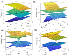
Figure S4: Effective band structures obtained by the disorder-averaged Green’s function method for four different random-flux strengths: (a) $U=0$, (b) $0.3\text{$\pi$}$, (c) $U_{c}=0.75\pi$, and (d) $1.2\pi$, respectively. $3.8\times 10^{5}$ configurations are considered. Other parameters are $L=26$, $t_{x}=0.2t$ and $t_{y}=0.6t$.

As shown by our numerical calculations (see Fig. 3 in the main text), the 2D SSH model with random flux can resemble the BBH model. The ground state of the half-filled 2D SSH model with random-flux strength $U=2\pi$ (zero mean flux on each plaquette) can be adiabatically mapped to that of the BBH model (with $\pi$ flux on each plaquette). To better understand how the random flux influences the system, we compare the 2D SSH model with the BBH model. In the clean case, the two models are given respectively by

$$H_{\mathrm{0}}({\bf k}) =(t_{x}+t\cos k_{x})\tau_{1}\sigma_{0}-t\sin k_{x}\tau_{2}\sigma_{3}+(t_{y}+t\cos k_{y})\tau_{1}\sigma_{1}-t\sin k_{y}\tau_{1}\sigma_{2},$$ (S3.6)

$$H_{\mathrm{BBH}}({\bf k}) =(t_{x}+t\cos k_{x})\tau_{1}\sigma_{3}+t\sin k_{x}\tau_{2}\sigma_{0}+(t_{y}+t\cos k_{y})\tau_{1}\sigma_{1}+t\sin k_{y}\tau_{1}\sigma_{2}.$$ (S3.7)

The two models share common matrices $\tau_{1}\sigma_{1}$ and $\tau_{1}\sigma_{2}$ (acting on the sublattice degrees of freedom). The 2D SSH model has two more matrices $\tau_{1}\sigma_{0}$ and $\tau_{2}\sigma_{3}$. Since the four matrices of the 2D SSH model do not all anticommute, the bulk system can have a gapless band structure. In contrast, the BBH model possesses two other additional matrices $\tau_{1}\sigma_{3}$ and $\tau_{2}\sigma_{0}$. Since the four matrices of the BBH model all anticommute, the bulk system has a fully gapped band structure. Thus, there are totally six different matrices in the two models.

The resemblance of our model with the BBH model implies that the self-energy $\Sigma({\bf k})$ due to the presence of random flux may be expanded in terms of

$$\Sigma({\bf k})=m_{x}\tau_{1}\sigma_{0}+m_{y}\tau_{1}\sigma_{1}+m_{p}\tau_{1}\sigma_{3}+f_{x}\tau_{2}\sigma_{3}+f_{y}\tau_{1}\sigma_{2}+f_{p}\tau_{2}\sigma_{0}.$$ (S3.8)

We choose this ansatz in the following. Thus, the effective Hamiltonian of our disorder-averaged system can be written as

$$H_{\mathrm{eff}}({\bf k}) =H_{0}({\bf k})+\Sigma({\bf k}).$$ (S3.9)

We demonstrate below that self-energy not only modifies the coefficients of the original matrices in the 2D SSH model but also introduces additional terms associated with new matrices ($\tau_{1}\sigma_{3}$ and $\tau_{2}\sigma_{0}$) to the Hamiltonian $H_{0}({\bf k})$. Importantly, it is momentum dependent and not diagonal in sublattice space. Note that $\Sigma({\bf k})$ may contain non-Hermitian components which give rise to the finite lifetimes of states. However, they are not important to our results and thus ignored.

We confirm the above ansatz by calculating $H_{\mathrm{eff}}({\bf k})$ numerically and extracting the corresponding coefficients of $\Sigma({\bf k})$, as shown in Fig. S5. Clearly, $\Sigma({\bf k})$ effectively modifies the coefficients of the four original matrices in $H_{0}({\bf k})$ and gives rise to the new terms associated with $\tau_{1}\sigma_{3}$ and $\tau_{2}\sigma_{0}$. Moreover, the coefficients in Eq. (S3.8) are highly momentum-dependent. This result indicates that the effective Hamiltonian $H_{\mathrm{eff}}({\bf k})$ can be regarded as a mixture of the 2D SSH model and the BBH model.

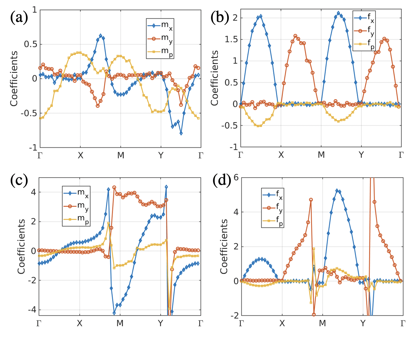
Figure S5: (a) Coefficients $m_{x,y,p}$ along the high symmetry lines for $U=0.3\pi$. (b) Coefficients $f_{x,y,p}$ along the high symmetry lines for $U=0.3\pi$. (c) Similar to (a) but for $U=1.2\pi$. (d) Similar to (b) but for $U=1.2\pi$. We choose $L=26$ and $3.8\times 10^{5}$ disorder configurations.

The modification to the original matrices and the emergence of the new matrices $\tau_{1}\sigma_{3}$ and $\tau_{2}\sigma_{0}$ in Eq. (S3.8) can be explained by the scattering of electrons by the random flux. To do so, we consider, for instance, the contribution (to the self-energy) from scattering processes of the lowest nonzero order. This contribution can be calculated as

$$\Sigma_{(2)}({\bf k})=\langle VG_{0}V\rangle_{\text{ave}},$$ (S3.10)

where $G_{0}$ is the bare Green’s function in the absence of flux and given by

$$G_{0}=\dfrac{f_{1}\Gamma_{1}+f_{2}\Gamma_{2}+f_{3}\Gamma_{3}+f_{4}\Gamma_{4}}{f_{1}^{2}+f_{2}^{2}+f_{3}^{2}+f_{4}^{2}},$$ (S3.11)

and $V$ is the modification due to the presence of random flux

$$V\equiv H_{\text{rand}}({\bf k},{\bf A})-H_{\mathrm{0}}({\bf k})=t(g_{3}\Gamma_{3}+g_{4}\Gamma_{4}).$$ (S3.12)

In the latter equation, ${\bf A}=(A_{x},A_{y})$ is the vector potential associated with the random flux. For concreteness, we choose the Landau gauge with $A_{x}=0$ and consider $\omega=0$. $\langle...\rangle_{\text{ave}}$ indicates the average over random flux configurations and the integral over internal variables; ${\bf k}$ acts as operator $-i\partial_{{\bf r}}$. We use the following shorthand notations

$$\Gamma_{1} \equiv\tau_{1}\sigma_{0},\ \ \Gamma_{2}=\tau_{2}\sigma_{3},\ \ \Gamma_{3}\equiv\tau_{1}\sigma_{1},\ \ \Gamma_{4}\equiv\tau_{1}\sigma_{2},$$

$$f_{1} \equiv-(t_{x}+t\cos k_{x}),\ \ f_{2}\equiv t\sin k_{x},\ \ f_{3}\equiv t_{y}+t\cos k_{y},\ \ f_{4}\equiv-t\sin k_{y},$$

$$g_{3} \equiv\cos(k_{y}-A_{y})-\cos k_{y},\ \ g_{4}\equiv-\sin(k_{y}-A_{y})+\sin k_{y}.$$ (S3.13)

This implies that

$$H_{0}({\bf k}) =-f_{1}\Gamma_{1}-f_{2}\Gamma_{2}+f_{3}\Gamma_{3}+f_{4}\Gamma_{4},$$

$$V({\bf k},{\bf A}) =t(g_{3}\Gamma_{3}+g_{4}\Gamma_{4}).$$ (S3.14)

Plugging Eqs. (S3.11) and (S3.12) into Eq. (S3.10), we find that

$$\Sigma_{(2)}({\bf k}) =t^{2}\langle(g_{3}\Gamma_{3}+g_{4}\Gamma_{4})(f_{1}\Gamma_{1}+f_{2}\Gamma_{2}+f_{3}\Gamma_{3}+f_{4}\Gamma_{4})\varLambda(g_{3}\Gamma_{3}+g_{4}\Gamma_{4})\rangle_{\text{ave}}$$

$$=\langle\mathcal{F}_{1}\rangle\Gamma_{1}+\langle\mathcal{F}_{2}\rangle\Gamma_{2}+\langle\mathcal{F}_{3}\rangle\Gamma_{3}+\langle\mathcal{F}_{4}\rangle\Gamma_{4}+\langle\mathcal{G}_{1}\rangle\tau_{1}\sigma_{3}+\langle\mathcal{G}_{2}\rangle\tau_{2}\sigma_{0},$$ (S3.15)

where $\varLambda=(f_{1}^{2}+f_{2}^{2}+f_{3}^{2}+f_{4}^{2})^{-1}$ and the corresponding coefficient functions are given by

$$\langle\mathcal{F}_{1}\rangle =t^{2}\langle g_{3}f_{1}\varLambda g_{3}+g_{4}f_{1}\varLambda g_{4}\rangle_{\text{ave}},$$

$$\langle\mathcal{F}_{2}\rangle =t^{2}\langle g_{3}f_{2}\varLambda g_{3}+g_{4}f_{2}\varLambda g_{4}\rangle_{\text{ave}},$$

$$\langle\mathcal{F}_{3}\rangle =t^{2}\langle g_{3}f_{3}\varLambda g_{3}+g_{3}f_{4}\varLambda g_{4}+g_{4}f_{4}\varLambda g_{3}-g_{4}f_{3}\varLambda g_{4}\rangle_{\text{ave}},$$

$$\langle\mathcal{F}_{4}\rangle =t^{2}\langle-g_{3}f_{4}\varLambda g_{3}+g_{3}f_{3}\varLambda g_{4}+g_{4}f_{3}\varLambda g_{3}+g_{4}f_{4}\varLambda g_{4}\rangle_{\text{ave}},$$

$$\langle\mathcal{G}_{1}\rangle =it^{2}\langle g_{3}f_{1}\varLambda g_{4}-g_{4}f_{1}\varLambda g_{3}\rangle_{\text{ave}},$$

$$\langle\mathcal{G}_{2}\rangle =it^{2}\langle g_{3}f_{2}\varLambda g_{4}-g_{4}f_{2}\varLambda g_{3}\rangle_{\text{ave}}.$$ (S3.16)

To derive Eq. (S3.15), we employ

$$\Gamma_{3}\Gamma_{1}\Gamma_{4} =-\Gamma_{4}\Gamma_{1}\Gamma_{3}=i\tau_{1}\sigma_{3},$$

$$\Gamma_{3}\Gamma_{2}\Gamma_{4} =-\Gamma_{4}\Gamma_{2}\Gamma_{3}=i\tau_{2}\sigma_{0}.$$ (S3.17)

Remarkably, $\Sigma_{(2)}({\bf k})$ has the same matrix structure as the ansatz, Eq. (S3.10). In a similar way, we can derive the contributions of higher order scattering processes. The emergence of the new matrices (i.e., nonzero $\langle\mathcal{G}_{1}\rangle$ and $\langle\mathcal{G}_{2}\rangle$) stems from the interplay between the intrinsic sublattice degrees of freedom and the fact that the magnetic flux couples to momentum.

Appendix S4 Conventional random flux model

In this section, we connect our results to the conventional random flux model which corresponds to $t_{x}=t_{y}=t$ in our model. For this limit, the model looses its inner degrees of freedom. Consequently, the spectrum reduces to $E({\bf k})=t(\cos k_{x}+\cos k_{y}),$ which is the spectrum of a conventional 2D electron gas.

It is known that the band center is delocalized in the conventional random flux model (Furusaki, 1999). In Fig. S6(a), we show clearly that the random flux cannot open a bulk gap around the band center at $E=0$. Correspondingly in Fig. S6(b), the LSR for states near the band center stays around $0.6$, confirming its delocalized nature. However, the states away from the band center are localized.

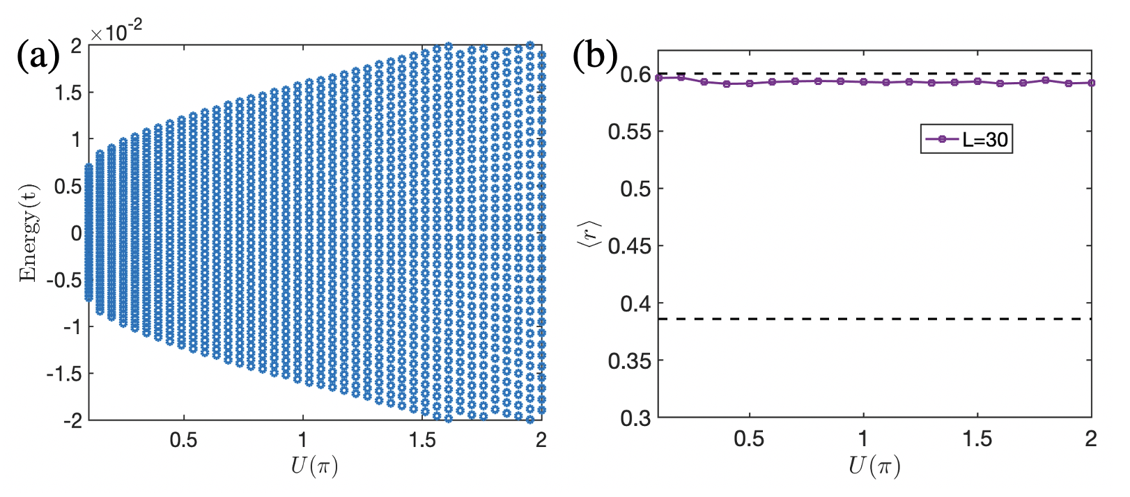
Figure S6: (a) Energy spectrum as a function of $U$ for the $t_{x}=t_{y}=t$ limit. 40 energy levels around zero energy are shown. (b) LSR as a function of $U$ near the band center for the $t_{x}=t_{y}=t$ limit . We take $L=40$ ($L=30$) and 200 (4000) disorder configurations in (a) [(b)].