Perturbations of giant magnons and single spikes in $\mathbb{R}\times S^{2}$

Abstract

Perturbations of giant magnons and single spikes in a $2+1$ dimensional $\mathbb{R}\times S^{2}$ background spacetime are analysed. Using the form of the giant magnon solution in the Jevicki-Jin gauge, the well-known Jacobi equation for small normal deformations of an embedded time-like surface are written down. Surprisingly, this equation reduces to a simple wave equation in a Minkowski background. The finiteness of perturbations and the ensuing stability of such giant magnons under small deformations are then discussed. It turns out that only the zero mode has finite deformations and is stable. Thereafter, we move on to explore the single spike solution in the Jevicki-Jin gauge. We obtain and solve the perturbation equation numerically and address stability issues.

1 Introduction

Rigidly rotating strings with cusps or spikes have been investigated earlier quite extensively in the context of cosmic strings BurdenTassie1: 1982 ; BurdenTassie2: 1982 ; BurdenTassie3: 1984 ; Burden: 1985 ; Embacher: 1992 ; rigid:1 ; rigid:2 ; rigid:3 ; Burden: 2008 ; ogawa:2008 . In its modern avatar, such rigidly rotating strings have been renamed as spiky strings. Their importance and relevance today is largely in the context of the AdS/CFT correspondence Maldacena:1997re . More than a decade ago, the spiky string solutions appeared through the seminal work of Kruczenski Kruczenski:2004wg , as a potential gravity dual to higher twist operators in string theory. The semiclassical aspect of these solutions arise through evaluating their energies, angular momenta and finding relations between them Gubser:2002tv . In providing meaningful input towards the realization of the gauge-gravity duality, the emergence of integrability on both sides have been quite useful and important. Classical and quantum integrability of the ${\cal N}$ = 4 Supersymmetric Yang-Mills (SYM) theory in the planar limit is mainly useful for the remarkable advances in understanding the theory Minahan:2002ve ; dolan ; nappi . The nonlocal conserved charges found on the string side Mandal:2002fs ; Bena:2003wd appear to have a counterpart in planar gauge theory at weak coupling within the spin-chain formulation for the dilatation operator. In this connection, Hoffman and Maldacena HM considered a special limit $(J\rightarrow\infty$, $\lambda$ = fixed, $p$ = fixed, $E-J$ = fixed), with $J$ being the angular momentum, $E$ the total energy, $p$ the momentum carried by the string in the spin chain and $\lambda$ the ‘t Hooft coupling constant. They considered operators of the form $O_{p}\sim\sum_{l}e^{ilp}(...ZZZWZZZ...)$, where the field $W$ is inserted at position $l$ along the spin-chain. In this limit, the problem of determining the spectrum on both (i.e. string and gauge theory) sides becomes simple. Such impurities are called “magnons” that propagate along the spin-chain with a conserved momentum $p$. In the large $\lambda$ limit the dispersion relation can be written in the form

$$E-J=\frac{\sqrt{\lambda}}{\pi}|\sin{\frac{p}{2}}|\,\,.$$

To describe these elementary excitations in the string theory side the authors in HM considered the string sigma model in AdS₅ $\times$ S ⁵ and have taken the large $\lambda$ limit. In this limit, the classical approximation is valid. Computing energy in this limit they found

$$E-J=\frac{\sqrt{\lambda}}{\pi}\sin{\frac{\Delta\phi}{2}}\,\,,$$

where $\Delta\phi$ represents a geometric angle in the string theory side. Now identifying $\Delta\phi=p$, one can have the perfect match between the two dispersion relations. Giant magnons can be visualised as a special limit of such spiky strings with shorter wavelengths. In ishizeki07 another limit called the single spike limit of rigidly rotating string the solution can be visualized as a string wound infinitely along the equator of $S^{2}$ with a single spike pointing towards the north pole. A large class of such spiky strings and giant magnons in various backgrounds have been studied, for example, in Kruczenski:2004wg ,Frolov:2003qc ; dorey1 ; chen1 ; chen2 ; russo ; hirano ; hofman07 ; swanson ; ishizeki07 ; arutyunov ; dorey2 ; ishizeki08 ; Biswas:2012wu ; Banerjee:2014gga ; Banerjee:2015nha . Given the above-stated importance of the spiky strings and giant magnons, it is worthwhile to look at the geometric properties of such string configurations from the world-sheet view point. Here following our earlier works bkp:2017 , bkp:2018 we study normal deformations (linearized) about the classical giant magnon solution in $\mathbb{R}\times S^{2}$ using the well-known Jacobi equations garriga: 1993 ; guven: 1993 ; frolov: 1994 ; capovilla: 1995 which govern normal deformations of an embedded surface. Earlier work in Frolov:2002av dealt with computation of quantum corrections to the energy spectrum, by expanding the supersymmetric action to quadratic order in fluctuations about the classical solution. The linearized perturbations of semiclassical strings are extremely instructive in matching the duality beyond the leading order classical solutions. The main motivations behind the perturbative solutions are multi-fold. On one hand, it helps in studying the stability properties of the string dynamics of the closed strings, and finding the quantum string corrections to the Wilson loop expectation value for the open string solutions and on the other hand, it helps us in determining the physical properties of topological defects. Apart from bkp:2017 ; bkp:2018 , related recent works on such perturbations can be found in forini:2015 ; rojas ; ida ; barik . The rest of this article is organised as follows. In Section 2, we briefly summarize the two different embeddings of the worldsheet and the rigidly rotating string solution in $\mathbb{R}\times S^{2}$. Section 3 is devoted to a study of the normal perturbations of the giant magnons in $\mathbb{R}\times S^{2}$. Section 4 is devoted to the single spike case. Our final concluding remarks appear in Section 5. Finally in the appendix we have briefly discussed the algorithm of finite difference method which we have used extensively in section 4.

2 Rigidly rotating strings in $\mathbb{R}\times S^{2}$: Kruczenski and Jevicki-Jin embeddings

The bosonic string worldsheet embedded in a $N$ dimensional curved spacetime with background metric functions $g_{ij}(x)$, is described by the well-known Nambu-Goto action given as,

$$S=-T\int d\tau\,\,d\sigma\sqrt{-\gamma}=-T\int d\tau\,\,d\sigma\sqrt{(\dot{x}\cdot x^{\prime})^{2}-\dot{x}^{2}{x^{\prime}}^{2}}\ .$$ (1)

Here $\gamma$ denotes the determinant of the induced metric $\gamma_{ab}=g_{ij}\partial_{a}x^{i}\partial_{b}x^{j}$ ($a,b=\sigma,\tau$). The $x^{i}(\tau,\sigma)$ are functions which describe the profile of the string worldsheet, as embedded in the target spacetime. Here $T$ denotes the string tension. We have used the notation: $\dot{x}=\partial_{\tau}x$,  $x^{\prime}=\partial_{\sigma}x$,   $(\dot{x}\cdot x^{\prime})=g_{ij}{\dot{x}}^{i}\,{x^{\prime}}^{j}$,  ${\dot{x}}^{2}=g_{ij}{\dot{x}}^{i}\,{\dot{x}}^{j}$ and ${x^{\prime}}^{2}=g_{ij}{x^{\prime}}^{i}\,{x^{\prime}}^{j}$.

Let us now turn to rigidly rotating strings in $\mathbb{R}\times S^{2}$ background. The three dimensional background line element is given as,

$$ds^{2}=-dt^{2}+d\theta^{2}+\sin^{2}\theta d\phi^{2}\,\,.$$ (2)

This $2+1$ dimensional spacetime is non-flat but has constant Ricci curvature. The value of $R$ is given as

$$R=2\,.$$ (3)

However this is not Einstein space for which one has

$$R_{ij}=\Lambda g_{ij}\,\,.$$ (4)

We may refer to the background space as one with constant positive curvature.

The embedding used in ishizeki07 is as follows,

$$t=\kappa\tau,\ \ \theta=\theta(\sigma),\ \ \phi=\omega\tau+\sigma\,\,.$$ (5)

Here $\omega$ and $\kappa$ are two parameters.

From the equations of motion one can arrive at the following first integral for $\theta$.

$$\theta^{\prime}=\frac{\kappa\sin\theta}{C}~{}\sqrt{\frac{\omega^{2}\sin^{2}\theta-C^{2}}{\kappa^{2}-\omega^{2}\sin^{2}\theta}}\,\,,$$ (6)

where $C$ is the integration constant.

As discussed in ishizeki07 equation (6) can have two distinct limits: 1) $|\omega|\rightarrow\kappa$ and  2) $|\omega|\rightarrow C$. Both these limits simplify the mathematical expressions. The first of these limits will give rise to the giant magnon solution which is identified by the following (magnon) dispersion relation,

$$E-J=\frac{\sqrt{\lambda}}{\pi}~{}|\sin{\frac{\Delta\phi}{2}}|\,\,.$$ (7)

In the dual field theory the $\Delta\phi$ is mapped onto momentum–hence the name ‘magnon’.

The second limit will give rise to what is called the single spike solution and described by a string wrapped around the equator, infinite number of times with a single spike pointing towards the pole of the $2$-sphere. Here we will focus on the giant magnon solution.

Here we work in the conformal gauge and use the embedding due to Jevicki and Jin (jevicki08, ), given as

$$t=\kappa\tilde{\tau}+f(\tilde{\sigma}),\hskip 7.22743pt\theta=\theta(\tilde{\sigma}),\hskip 7.22743pt\phi=\omega\tilde{\tau}+g(\tilde{\sigma})\,\,.$$ (8)

where $\tilde{\tau}$ and $\tilde{\sigma}$ are the worldsheet coordinates. We retain $\kappa$, $\omega$ as in the embedding mentioned before in equation (5).

In conformal gauge, we have the following Virasoro constraint equations

$$g_{ij}({\dot{x}}^{i}{\dot{x}}^{j}+{x^{\prime}}^{i}{x^{\prime}}^{j})=0,\hskip 21.68121ptg_{ij}{\dot{x}}^{i}{x^{\prime}}^{j}=0\ .$$ (9)

In such a gauge, the string equations of motion obtained by varying the action with respect to $x^{i}$, take the form:

$${\ddot{x}}^{i}-{x^{i^{\prime\prime}}}+\Gamma^{i}_{jk}\left({\dot{x}}^{j}{\dot{x}}^{k}-{x}^{j\prime}{x}^{k\prime}\right)=0\ .$$ (10)

Using the above ansatz and after some simplifications, we have the following equation for $\theta(\tilde{\sigma})$,

$$\theta^{\prime}=\pm\sqrt{(\kappa^{2}+a^{2})-(\omega^{2}\sin^{2}\theta+\frac{C^{2}}{\sin^{2}\theta})}\,\,,$$ (11)

which also satisfies one of the Virasoro conditions. Note that the prime on the L. H. S. above is w.r.t. $\tilde{\sigma}$.

From the other Virasoro condition (9) we have

$$\kappa~{}a=\omega~{}C\,\,.$$ (12)

Using this equation for replacing the parameter $a$, we rewrite the equation for $\theta$ as

$$\theta^{\prime}=\pm\frac{1}{\kappa\sin\theta}\sqrt{(\kappa^{2}-\omega^{2}\sin^{2}\theta)(\kappa^{2}\sin^{2}\theta-C^{2})}\,\,$$ (13)

2.1 Giant magnons in $\mathbb{R}\times S^{2}$

In the giant magnon limit $|\omega|\rightarrow\kappa$, from equation (12) we have

$$a=C\,\,.$$ (14)

Equation (11) will take the following form

$$\theta^{\prime}=\pm\frac{\cos\theta}{\sin\theta}\sqrt{\omega^{2}\sin^{2}\theta-C^{2}}\,\,.$$ (15)

The equations of motion and the Virasoro constraints give us the following conditions,

$$f^{\prime}(\tilde{\sigma})=a\hskip 14.45377pt;\hskip 14.45377ptg^{\prime}(\tilde{\sigma})=\frac{C}{\sin^{2}\theta}\,\,.$$ (16)

Integrating equation (15) we have the expression for $\theta$

$$\cos\theta=\frac{\alpha}{\cosh\alpha\omega\tilde{\sigma}}$$ (17)

where $\alpha^{2}=1-\frac{c^{2}}{\omega^{2}}$. Similarly $f(\tilde{\sigma})$ and $g(\tilde{\sigma})$ will be of the following form

$$f(\tilde{\sigma}) = C\tilde{\sigma}+b\,\,,$$ (18)

$$g(\tilde{\sigma}) = C\tilde{\sigma}\mp\tan^{-1}\left(\frac{\sqrt{1-\alpha^{2}}}{\alpha}\coth\,\omega\alpha\tilde{\sigma}\right)$$ (19)

Without loss of generality we can set $b=0$.

The relation between the two embeddings can be understood as follows. For embedding (5) the induced metric is not diagonal while for the conformal gauge it is so. The $\tau,~{}\sigma$ in the non-diagonal case are related to those in the diagonal case as follows:

$$\tau=\tilde{\tau}+\frac{f(\tilde{\sigma})}{\omega},\,\,\,\,\hskip 14.45377pt\sigma=g(\tilde{\sigma})-f(\tilde{\sigma})\,\,.$$ (20)

We can transform the derivative in the L. H. S of the equation for $\theta^{\prime}$ quoted above into a derivative w.r.t. $\sigma$ by using the above relation. It is easy to check that the equation in the Jevicki-Jin gauge goes over to that in the Kruczenski gauge. Further, using the relation between $\sigma$ and $\tilde{\sigma}$ one can convert the solution for $\theta(\tilde{\sigma})$ to the solution $\theta(\sigma)$ in the Kruczenski gauge. It is important to realise that while the $\sigma$ runs from $\theta_{0}$ to $\frac{\pi}{2}$ (or $-\theta_{0}$ to $-\frac{\pi}{2}$, $\sin\theta_{0}=\frac{C}{\omega}$), the $\tilde{\sigma}$ runs from $0$ to $\pm\infty$. The values of the spacetime coordinate $\theta$ in both gauges run from $\theta_{0}$ to $\frac{\pi}{2}$ (or their negative valued counterparts).

We now turn towards examining the stability of the above string configurations by studying their normal deformations.

3 Perturbations and stability of giant magnons in $\mathbb{R}\times S^{2}$

Before investigating the perturbation equations for our specific solutions, let us briefly recall the well-known Jacobi equations which deal with perturbations of extremal worldsheets.

3.1 Jacobi equations for extremal surfaces

Given that $x^{i}(\tau,\sigma)$ are the embedding functions and $g_{ij}$ the background metric, the tangent vectors to the worldsheet are

$$e^{i}_{\tau}=\partial_{\tau}x^{i},\hskip 14.45377pte^{i}_{\sigma}=\partial_{\sigma}x^{i},$$ (21)

Thus, the induced line element turns out to be,

$$\gamma_{ab}=g_{ij}e^{i}_{a}e^{j}_{b}\ ,$$ (22)

where the $a,b...$ denote worldsheet indices (here $\tau$, $\sigma$). The worldsheet normals $n^{i}_{(\alpha)}$ satisfy the relations

$$g_{ij}n^{i}_{(\alpha)}n^{j}_{(\beta)}=\delta_{\alpha\beta},\hskip 14.45377ptg_{ij}n^{i}_{(\alpha)}e^{j}_{a}=0\ ,$$ (23)

where $\alpha=1..,N-2$ and $N$ is the dimension of the background spacetime. The last condition holds for all $\alpha$ and $a$. Extrinsic curvature tensor components $K_{ab}^{(\alpha)}$ along each normal $n^{i}_{(\alpha)}$ of the embedded worldsheet are

$$K_{ab}^{(\alpha)}=-g_{ij}(e^{k}_{a}\nabla_{k}e^{i}_{b})n^{j(\alpha)}\ .$$ (24)

The equations of motion lead to the condition, $K^{(\alpha)}=\gamma^{ab}K_{ab}^{(\alpha)}=0$ for an extremal worldsheet. Thus extremal surfaces are those for which the trace of the extrinsic curvature tensor along each normal is zero. Normal deformations are denoted as $\phi^{(\alpha)}$ along each normal. Therefore, the deformations constitute a set of scalar fields. More explicitly, the deformation of each coordinate is

$$\delta x^{i}=\phi^{(\alpha)}n^{i}_{(\alpha)}\ ,$$ (25)

which is the perturbation of the worldsheet (i.e. $x^{i}\rightarrow x^{i}+\delta x^{i}$). For a worldsheet with $\gamma^{ab}K_{ab}^{(\alpha)}=0$ satisfying the equations of motion and the Virasoro constraints, the scalars $\phi^{i}_{(\alpha)}$ satisfy the Jacobi equations given as.

$$\frac{1}{\Omega^{2}}\left(-\frac{\partial^{2}}{\partial\tau^{2}}+\frac{\partial^{2}}{\partial\sigma^{2}}\right)\phi^{(\alpha)}+\left(M^{2}\right)^{(\alpha)}_{(\beta)}\phi^{(\beta)}=0\ ,$$ (26)

where

$$\left(M^{2}\right)^{(\alpha)}_{(\beta)}=K_{ab}^{(\alpha)}K^{ab}_{(\beta)}+R_{ijkl}e^{j}_{a}e^{l\,\,a}n^{i\,\,(\alpha)}n^{k}_{(\beta)}\ ,$$ (27)

and $\Omega^{2}(\tau,\sigma)$ is the conformal factor of the conformally flat form of the worldsheet line element. The Jacobi equations are obtained by constructing the second variation of the worldsheet action. Thus, solving these equations for the perturbation scalars one can analyse the stability properties of the extremal worldsheet. In other words, a stable worldsheet will correspond to an oscillatory character for the $\delta x^{i}$ defined above.

Note further that the Jacobi equations are like a family of coupled, variable ‘mass’ wave equations for the scalars $\phi^{(\alpha)}$. They are a generalisation of the familiar geodesic deviation equation for geodesic curves in a Riemannian geometry. Usually, these equations are quite complicated and not easily solvable, even for the simplest cases. It turns out that for the string configurations under consideration here, we do find analytical solutions.

In a more general context, the worldsheet covariant derivative does have a term arising from the extrinsic twist potential (normal fundamental form) which is given as: $\omega_{a}^{\,\,\alpha\beta}=g_{ij}\,\left(e^{k}_{a}\nabla_{k}\,n^{i\,\alpha}\right)\,n^{j\,\beta}$. For codimension one surfaces, i.e. hypersurfaces (as is the case here), the $\omega_{a}^{\alpha\beta}$ are all identically zero.

3.2 The case of giant magnons in $\mathbb{R}\times S^{2}$

We will only look at the giant magnon configurations in the $\mathbb{R}\times S^{2}$ and compute the perturbations. To proceed, we first write down the normal and the extrinsic curvature for the world sheet configurations, in the Jevicki-Jin gauge stated earlier. Below, we will use $\tilde{\sigma}$, $\tilde{\tau}$ for the Jevicki-Jin gauge.

The induced metric is given as:

$$ds^{2}=\omega^{2}\cos^{2}\theta\left(-d{\tilde{\tau}}^{2}+d{\tilde{\sigma}}^{2}\right)=\frac{\omega^{2}\alpha^{2}}{\cosh^{2}{\tilde{\sigma}}}~{}\left(-d{\tilde{\tau}}^{2}+d{\tilde{\sigma}}^{2}\right)\,\,.$$ (28)

The tangent vectors to the worldsheet are given as:

$$e^{i}_{\tilde{\tau}}=\left(\omega,~{}0,~{}\omega\right)\hskip 14.45377pt;\hskip 14.45377pte^{i}_{\tilde{\sigma}}=\left(f^{\prime},~{}\theta^{\prime},~{}g^{\prime}\right)\,\,.$$ (29)

The normal to the worldsheet is given as:

$$n^{i}=\left(\frac{\sqrt{\omega^{2}\sin^{2}\theta-C^{2}}}{\omega\cos\theta},~{}-\frac{C}{\omega\sin\theta},~{}\frac{\sqrt{\omega^{2}\sin^{2}\theta-C^{2}}}{\omega\sin^{2}\theta\cos\theta}\right)$$ (30)

The extrinsic curvature tensor which is defined as $K_{ab}^{(\alpha)}=-g_{ij}(e^{k}_{a}\nabla_{k}e^{i}_{b})n^{j(\alpha)}$, turns out to be

$$K_{ab}=\begin{pmatrix}-C\omega\cos\theta&-\omega^{2}\cos\theta\cr-\omega^{2}\cos\theta&-C\omega\cos\theta\end{pmatrix}.$$ (31)

Note that the trace of $K_{ab}$ vanishes (i.e $\gamma^{ab}K_{ab}=0$), which is the classical equation of motion. Hence the quantity $K_{ab}K^{ab}$ is given as:

$$K_{ab}K^{ab}=\frac{2(C^{2}-\omega^{2})}{\omega^{2}\cos^{2}\theta}\,\,.$$ (32)

Similarly one can write down the contribution from the Riemann tensor term in the perturbation equation as follows:

$$R_{ijkl}~{}e^{j}_{a}~{}e^{l\,\,a}~{}n^{i\,\,(\alpha)}~{}n^{k}_{(\beta)}=\frac{(\omega^{2}-C^{2})}{\omega^{2}\cos^{2}\theta}\delta^{\alpha}_{\beta}\,\,.$$ (33)

Using all of the above-stated quantities which appear in the perturbation equation and after some lengthy algebra, one arrives at the following simple equation for the perturbation scalar $\phi$

$$\left(-\partial_{\tilde{\tau}}^{2}+\partial_{\tilde{\sigma}}^{2}\right)\phi+\left(C^{2}-\omega^{2}\right)\phi=0\,\,.$$ (34)

Let us now use the ansatz

$$\phi(\tilde{\tau},\tilde{\sigma})=\epsilon e^{i\beta\tilde{\tau}}~{}P(\tilde{\sigma})\,\,,$$ (35)

where $\beta$ is the eigenvalue and $\epsilon$, a constant which we may relate to the amplitude of the perturbation. It must be emphasized that $\epsilon$ has to be small in value (i.e. $\epsilon<<1$) in order to ensure that the deformation is genuinely a small perturbation.

Equation (34) will take the following form after using the above ansatz

$$\frac{d^{2}P}{d\tilde{\sigma}^{2}}+\left(\beta^{2}+C^{2}-\omega^{2}\right)P=0\,\,.$$ (36)

Depending on the sign of $\beta^{2}+C^{2}-\omega^{2}$, equation (58) can have oscillatory or exponential general solutions given as

$$P_{1}(\tilde{\sigma}) = A\cos M\tilde{\sigma}+B\sin M\tilde{\sigma}$$ (37)

$$P_{2}(\tilde{\sigma}) = Ae^{-M\tilde{\sigma}}+Be^{M\tilde{\sigma}}$$ (38)

where $M^{2}=\beta^{2}+C^{2}-\omega^{2}=\beta^{2}-\alpha^{2}\omega^{2}$. Now $M^{2}>0$ is for the oscillatory solution and $M^{2}<0$ is for the exponential solution.

Thus, our complete solution will be of the following form

$$\phi(\tilde{\tau},\tilde{\sigma})=\epsilon~{}e^{i\beta\tilde{\tau}}P_{1,2}\,\,$$ (39)

where, one will have to choose either $P_{1}$ or $P_{2}$.

Using the solution for $\theta$ (equation (17)) we can write the equation for the normal $n^{i}$ (equation (30)) as

$$n^{i}=\left(\sinh\bar{\sigma},~{}-\frac{C}{\omega}\frac{\cosh\bar{\sigma}}{\sqrt{\cosh^{2}\bar{\sigma}-\alpha^{2}}},~{}\frac{\sinh\bar{\sigma}\cosh^{2}\bar{\sigma}}{\cosh^{2}\bar{\sigma}-\alpha^{2}}\right)\,\,.$$ (40)

Here $\bar{\sigma}=\alpha~{}\omega~{}\tilde{\sigma}$.

Notice that the $n^{0}$ and $n^{2}$ have an overall $\sinh\bar{\sigma}$ which diverges as $\bar{\sigma}$ tends to infinity. Now if we consider the solution $P_{1}(\tilde{\sigma})$ one can clearly see that $P_{1}(\tilde{\sigma})\sinh\bar{\sigma}$ will grow exponentially with $\tilde{\sigma}$ and thus we end up with an unstable solution. Hence one needs to look for the other solution $P_{2}(\tilde{\sigma})$. One can see from equation (38) that $P_{2}(\tilde{\sigma})$ has two terms, one is exponentially decaying with $\tilde{\sigma}$ while the other one is exponentially growing with $\tilde{\sigma}$. Since we are working here with an open string worldsheet, $\tilde{\sigma}$ runs from $0$ to $\infty$. We can impose a boundary condition on $\phi(\tilde{\tau},\tilde{\sigma})$ by considering that as $\tilde{\sigma}$ goes to $\infty$ the perturbation will vanish i.e: $\phi(\tilde{\tau},\tilde{\sigma})\rightarrow 0$ as $\tilde{\sigma}\rightarrow\infty$ which should follow from $P_{2}(\tilde{\sigma})\rightarrow 0$ (at $\tilde{\sigma}\rightarrow\infty$). To have $P_{2}(\tilde{\sigma})\rightarrow 0$ at $\tilde{\sigma}\rightarrow\infty$ we require $B=0$. Thus, we can safely choose the exponentially damped solution, i.e. $P_{2}\propto e^{-M\tilde{\sigma}}$. Multiplying this $P_{2}$ by $\sinh\bar{\sigma}$ would result in

$$P_{2}\sinh\bar{\sigma}=\frac{1}{2}e^{-M\tilde{\sigma}}\left(e^{\alpha\omega\tilde{\sigma}}-e^{-\alpha\omega\tilde{\sigma}}\right)=\frac{1}{2}\left(e^{-(M-\alpha\omega)\tilde{\sigma}}-e^{-(M+\alpha\omega)\tilde{\sigma}}\right)$$ (41)

From equation (41) we can say that to get an exponentially decaying solution of $\tilde{\sigma}$ one must have $M\geq\alpha\omega$ which means $\beta^{2}=\alpha^{2}\omega^{2}-M^{2}<0$. However, from equation (35) one can see that if $\beta^{2}<0$ then $\phi(\tilde{\tau},\tilde{\sigma})$ will give rise to exponentially growing (or decaying) solutions in $\tilde{\tau}$. To get a solution which is oscillatory in $\tilde{\tau}$ or independent of $\tilde{\tau}$ one must have $\alpha\omega\geq M$, which immediately leads to a solution growing exponentially with $\tilde{\sigma}$, if $\alpha\omega>M$. Thus, the only possibility to have a finite solution is $\beta=0$.

The perturbations ($\delta x^{i}=\phi^{\alpha}n^{i}_{\alpha}$) therefore, turn out to be,

$$\delta t = \phi(\tilde{\tau},\tilde{\sigma})n^{0}=\epsilon~{}Ae^{-\bar{\sigma}}\sinh\bar{\sigma}\,\,,$$ (42)

$$\delta\theta = \phi(\tilde{\tau},\tilde{\sigma})n^{1}=-\epsilon~{}Ae^{-\bar{\sigma}}\frac{C}{\omega}~{}\frac{\cosh\bar{\sigma}}{\sqrt{\cosh^{2}\bar{\sigma}-\alpha^{2}}}\,\,,$$ (43)

$$\delta\phi = \phi(\tilde{\tau},\tilde{\sigma})n^{2}=\epsilon~{}Ae^{-\bar{\sigma}}~{}\frac{\sinh\bar{\sigma}\cosh^{2}\bar{\sigma}}{\cosh^{2}\bar{\sigma}-\alpha^{2}}\,\,.$$ (44)

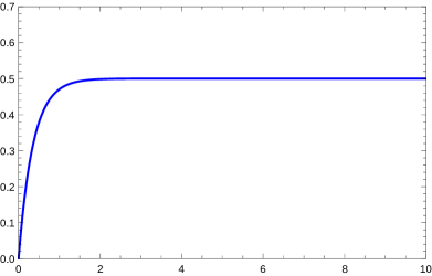
Figure 1: Plot of $\delta t$ for $A=1$,  $\omega=\sqrt{3}$,  $C=1$

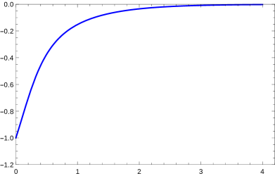
Figure 2: Plot of $\delta\theta$ for $A=1$,  $\omega=\sqrt{3}$,  $C=1$

All the perturbations are finite over the domain of $\tilde{\sigma}$. Note that there is no $\tilde{\tau}$ dependence since we have $\beta=0$. It is therefore only the zero mode of the perturbation which is stable. All higher modes will basically decay or grow in time (imaginary $\beta$). Figures 2,  2 and 4 have shown the perturbations $\delta t$,  $\delta\theta$ and  $\delta\phi$ respectively for $A=1$,  $\omega=\sqrt{3}$ and $C=1$. One can easily observe from the solutions and the figures that these perturbations are always finite. Hence the giant magnon is stable for the zero mode. Let us now try to understand how this perturbation affects the string profile. The perturbed embedding will be given as:

$$t^{\prime} = t+\delta t=\omega\tilde{\tau}+C\tilde{\sigma}+\delta t\,\,,$$ (45)

$$\theta^{\prime} = \theta+\delta\theta=\cos^{-1}\frac{\alpha}{\cosh\bar{\sigma}}+\delta\theta\,\,,$$ (46)

$$\phi^{\prime} = \phi+\delta\phi=\omega\tilde{\tau}+g(\tilde{\sigma})+\delta\phi\,\,.$$ (47)

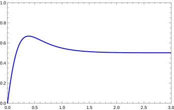
Figure 3: Plot of $\delta\phi$ for $A=1$,  $\omega=\sqrt{3}$,  $C=1$

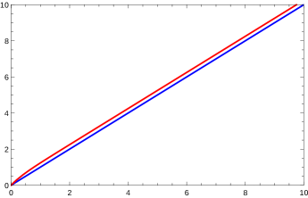
Figure 4: Plot of perturbed (red) and un-perturbed (blue) $t$- profile with $\tilde{\tau}=0$ for $A=1$,  $\omega=\sqrt{3}$,  $C=1$ and $\epsilon=0.5$

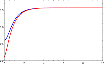
Figure 5: Plot of perturbed (red) and un-perturbed (blue) $\theta$-profile with $\tilde{\tau}=0$ for $A=1$,  $\omega=\sqrt{3}$,  $C=1$ and $\epsilon=0.5$

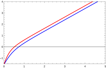
Figure 6: Plot of perturbed (red) and un-perturbed (blue) $\phi$-profile with $\tilde{\tau}=0$ for $A=1$,  $\omega=\sqrt{3}$,  $C=1$ and $\epsilon=0.5$

Figures 4,  6 and 6 describe the perturbed profiles for $t$,  $\theta$ and $\phi$ respectively for $\tilde{\tau}=0$. Here the blue curve describes the original un-perturbed profile whereas the red curve describes the perturbed profile. We have taken the amplitude of perturbation $\epsilon=0.5$. One notices clearly that over the entire domain of $\tilde{\sigma}$, the perturbed profile is finite for finite $\tilde{\sigma}$, but different from the unperturbed one. Thus, the stability of the giant magnon is guaranteed through the stability of the zero mode fluctuation, for all values of $\tilde{\tau}$.

4 Single spike solution and perturbation in $\mathbb{R}\times S^{2}$

In the single spike limit $|\omega|\rightarrow C$, from equation (12) we have

$$a=\frac{C^{2}}{\kappa}\,\,.$$ (48)

Equation (11) will take the following form

$$\theta^{\prime}=\pm\frac{1}{\kappa\sin\theta}\sqrt{(\kappa^{2}-C^{2}\sin^{2}\theta)(\kappa^{2}\sin^{2}\theta-C^{2})}\,\,.$$ (49)

The equations of motion and the Virasoro constraints give us the following conditions,

$$f^{\prime}(\tilde{\sigma})=a\hskip 14.45377pt;\hskip 14.45377ptg^{\prime}(\tilde{\sigma})=\frac{C}{\sin^{2}\theta}\,\,.$$ (50)

Integrating equation (49) we can write

$$\sigma=\pm\frac{\kappa}{\sqrt{\kappa^{2}-C^{2}}}~{}F\left(\sin^{-1}{\frac{\kappa\cos\theta}{\sqrt{\kappa^{2}-C^{2}}},~{}-\frac{C^{2}}{\kappa^{2}}}\right)\,\,.$$ (51)

Where $F$ is the elliptic integral of first kind. Now we can invert this expression by using the Jacobi elliptic functions. So the final form of $\theta$ will be

$$\cos\theta=\frac{\sqrt{\kappa^{2}-C^{2}}}{\kappa}~{}{\rm sn}(u,\tilde{\kappa})\,\,.$$ (52)

Now in equation (52) the variable $u$ and the modulus $\tilde{\kappa}$ is defined as

$$u=\pm\frac{\sqrt{\kappa^{2}-C^{2}}}{\kappa}~{}\tilde{\sigma}=\pm\sqrt{1+\tilde{\kappa}}~{}\tilde{\sigma}\hskip 14.45377pt;\hskip 14.45377pt\tilde{\kappa}=-\frac{C^{2}}{\kappa^{2}}\,\,.$$ (53)

4.1 Perturbations and stability of single spike in $\mathbb{R}\times S^{2}$

The induced metric is given as:

$$ds^{2}=(\kappa^{2}-C^{2}\sin^{2}\theta)\left(-d{\tilde{\tau}}^{2}+d{\tilde{\sigma}}^{2}\right)\,\,.$$ (54)

The tangent vectors to the worldsheet are given as:

$$e^{i}_{\tilde{\tau}}=\left(\kappa,~{}0,~{}C\right)\hskip 14.45377pt;\hskip 14.45377pte^{i}_{\tilde{\sigma}}=\left(f^{\prime},~{}\theta^{\prime},~{}g^{\prime}\right)\,\,.$$ (55)

The normal to the worldsheet is given as:

$$n^{i}=\left(\frac{C}{\kappa}\frac{\sqrt{\kappa^{2}\sin^{2}\theta-C^{2}}}{\sqrt{\kappa^{2}-C^{2}\sin^{2}\theta}},~{}-\frac{C}{\kappa\sin\theta},~{}\frac{\sqrt{\kappa^{2}\sin^{2}\theta-C^{2}}}{\sin^{2}\theta\sqrt{\kappa^{2}-C^{2}\sin^{2}\theta}}\right)$$ (56)

The extrinsic curvature tensor which is defined as $K_{ab}^{(\alpha)}=-g_{ij}(e^{k}_{a}\nabla_{k}e^{i}_{b})n^{j(\alpha)}$, turns out to be

$$K_{ab}=\begin{pmatrix}-\frac{C^{3}}{\kappa}\cos\theta&-C\kappa\cos\theta\cr-C\kappa\cos\theta&-\frac{C^{3}}{\kappa}\cos\theta\end{pmatrix}.$$ (57)

Using all of the above-stated quantities which appear in the perturbation equation and after some lengthy algebra, one arrives at the following simple equation for the perturbation scalar $\phi$

$$\left(-\partial_{\tilde{\tau}}^{2}+\partial_{\tilde{\sigma}}^{2}\right)\phi+\left(\frac{(\kappa^{4}-C^{4})(\kappa^{2}-C^{2}-C^{2}\sin^{2}\theta)}{\kappa^{2}(\kappa^{2}-C^{2}+C^{2}\cos^{2}\theta)}\right)\phi=0\,\,.$$ (58)

Let us now use the same ansatz as before

$$\phi(\tilde{\tau},\tilde{\sigma})=\epsilon e^{i\beta\tilde{\tau}}~{}P(\tilde{\sigma})\,\,,$$ (59)

where $\beta$ is the eigenvalue and $\epsilon$, a constant which we may relate to the amplitude of the perturbation. It must be emphasized that $\epsilon$ has to be small in value (i.e. $\epsilon<<1$) in order to ensure that the deformation is genuinely a small perturbation.

Using the previous ansatz to separate the $\tilde{\tau}$ and $\tilde{\sigma}$ part and exploiting equation (52) we can write down the equation for $P(\tilde{\sigma})$ as

$$\frac{d^{2}P}{du^{2}}+\left(\tilde{\beta}^{2}+\frac{(1-\tilde{\kappa})(1+\tilde{\kappa}~{}{\rm sn}^{2}u)}{(1+\tilde{\kappa})(1-\tilde{\kappa}~{}{\rm sn}^{2}u)}\right)P=0$$ (60)

Where $\tilde{\beta}$ is defined as $\tilde{\beta}^{2}=\frac{\beta^{2}\kappa^{2}}{\kappa^{2}-C^{2}}=\frac{\beta^{2}}{1+\tilde{\kappa}}$.

We can examine the nature of the potential $V(u)=\frac{(1-\tilde{\kappa})(1+\tilde{\kappa}~{}{\rm sn}^{2}u)}{(1+\tilde{\kappa})(1-\tilde{\kappa}~{}{\rm sn}^{2}u)}$ graphically by plotting it explicitly. Before that some points need to be mentioned: 1) Since $\tilde{\sigma}$ runs from $0$ to $\pm\infty$ so is $u$ except at $\tilde{\kappa}=-1$ where $u=0$ , one can see that from eqn (53), which is clearly justified from the condition of Lorenzian signature of the induced metric, 2) From (53) one can see that $-1<\tilde{\kappa}\leq 0$.

Plots of $V(u)$ have been shown in figures (7). Figure (7) shows the nature of the potential $V(u)$ in general for three different values of $\tilde{\kappa}$: 1) $\tilde{\kappa}=-0.05$ which is shown by the blue curve, 2)$\tilde{\kappa}=-0.1$ which is shown by the green curve and 3) $\tilde{\kappa}=-0.5$ which is shown by the red curve. From all these three curves one can see that the potential is of periodic nature.

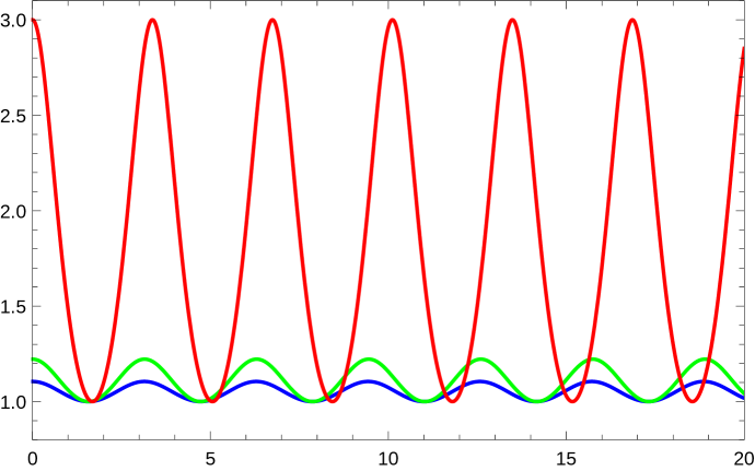
Figure 7: Plot of $V(u)$ for three different values of $\tilde{\kappa}$: 1) $\tilde{\kappa}=-0.05$ (blue), 2) $\tilde{\kappa}=-0.1$ (green) & 3) $\tilde{\kappa}=-0.5$ (red)

4.2 Solution of the perturbation equation

We have solved the perturbation equation (60) numerically using the finite difference method. We transform the above differential equation into a set of algebraic equations represented in the form of a matrix. We compute the eigenvalues and eigen-vectors for different cases. Here we consider mainly three different cases: 1) $\tilde{\kappa}=-0.05$, 2) $\tilde{\kappa}=-0.1$ and 3) $\tilde{\kappa}=-0.5$. The corresponding potential functions are shown in Figure 7 (the blue, green and red curves respectively).

Table 1: Eigenvalues for $\tilde{\kappa}=-0.05$

$\tilde{\kappa}$	N	$\lambda_{0}$	$\lambda_{1}$	$\lambda_{2}$	$\lambda_{3}$	$\lambda_{4}$
	$150$	$-1.05231984$	$2.94240006$	$2.94271174$	$14.91869654$	$14.91869660$
	$200$	$-1.05231981$	$2.94265559$	$2.94296730$	$14.92278399$	$14.92278406$
	$250$	$-1.05231980$	$2.94277387$	$2.94308559$	$14.92467619$	$14.92467625$
$-0.05$	$300$	$-1.05231980$	$2.94283812$	$2.94314984$	$14.92570412$	$14.92570418$
	$350$	$-1.05231979$	$2.94287686$	$2.94318859$	$14.92632395$	$14.92632401$
	$400$	$-1.05231979$	$2.94290201$	$2.94321374$	$14.92672626$	$14.92672632$
	$450$	$-1.05231979$	$2.94291925$	$2.94323098$	$14.92700209$	$14.92700215$
	$500$	$-1.05231979$	$2.94293158$	$2.94324331$	$14.92719939$	$14.92719945$

Table 2: Eigenvalues for $\tilde{\kappa}=-0.1$

$\tilde{\kappa}$	N	$\lambda_{0}$	$\lambda_{1}$	$\lambda_{2}$	$\lambda_{3}$	$\lambda_{4}$
	$150$	$-1.10987439$	$2.87095432$	$2.87219004$	$14.80231858$	$14.80231957$
	$200$	$-1.10987429$	$2.87120887$	$2.87244469$	$14.80639068$	$14.80639168$
	$250$	$-1.10987425$	$2.87132670$	$2.87256257$	$14.80827577$	$14.80827677$
$-0.1$	$300$	$-1.10987422$	$2.87139071$	$2.87262660$	$14.80929984$	$14.80930084$
	$350$	$-1.10987421$	$2.87142930$	$2.87266521$	$14.80991735$	$14.80991835$
	$400$	$-1.10987420$	$2.87145435$	$2.87269027$	$14.81031815$	$14.81031915$
	$450$	$-1.10987419$	$2.87147153$	$2.87270745$	$14.81059294$	$14.81059394$
	$500$	$-1.10987418$	$2.87148381$	$2.87271974$	$14.81078949$	$14.81079049$

Table 3: Eigenvalues for $\tilde{\kappa}=-0.5$

$\tilde{\kappa}$	N	$\lambda_{0}$	$\lambda_{1}$	$\lambda_{2}$	$\lambda_{3}$	$\lambda_{4}$
	$150$	$-2.00227136$	$1.65322654$	$1.65625830$	$12.02953349$	$12.03027567$
	$200$	$-2.00226233$	$1.65345610$	$1.65647916$	$12.03309099$	$12.03383350$
	$250$	$-2.00225814$	$1.65356236$	$1.65658139$	$12.03473785$	$12.03548050$
$-0.5$	$300$	$-2.00225587$	$1.65362008$	$1.65663693$	$12.03563250$	$12.03637524$
	$350$	$-2.00225450$	$1.65365488$	$1.65667041$	$12.03617197$	$12.03691476$
	$400$	$-2.00225361$	$1.65367747$	$1.65669215$	$12.03652211$	$12.03726494$
	$450$	$-2.00225300$	$1.65369296$	$1.65670705$	$12.03676218$	$12.03750502$
	$500$	$-2.00225256$	$1.65370404$	$1.65671770$	$12.03693389$	$12.03767675$

Table 4: $\Delta\lambda$ for $\tilde{\kappa}=-0.05$

$\Delta\lambda$	$\Delta\lambda_{0}$	$\Delta\lambda_{1}$	$\Delta\lambda_{2}$	$\Delta\lambda_{3}$	$\Delta\lambda_{4}$
$|\lambda(200)-\lambda(150)|$	$3.0\times 10^{-8}$	$2.55\times 10^{-4}$	$2.55\times 10^{-4}$	$4.1\times 10^{-3}$	$4.1\times 10^{-3}$
$|\lambda(250)-\lambda(200)|$	$1.0\times 10^{-8}$	$1.2\times 10^{-4}$	$1.2\times 10^{-4}$	$1.9\times 10^{-3}$	$1.9\times 10^{-3}$
$|\lambda(300)-\lambda(250)|$	$0.0\times 10^{-8}$	$0.6\times 10^{-4}$	$0.64\times 10^{-4}$	$1.0\times 10^{-3}$	$1.0\times 10^{-3}$
$|\lambda(350)-\lambda(300)|$	$0.0\times 10^{-8}$	$0.30\times 10^{-4}$	$0.38\times 10^{-4}$	$0.6\times 10^{-3}$	$0.62\times 10^{-3}$
$|\lambda(400)-\lambda(350)|$	$0.0\times 10^{-8}$	$0.2\times 10^{-4}$	$0.25\times 10^{-4}$	$0.4\times 10^{-3}$	$0.4\times 10^{-3}$
$|\lambda(450)-\lambda(400)|$	$0.0\times 10^{-8}$	$0.17\times 10^{-4}$	$0.17\times 10^{-4}$	$0.27\times 10^{-3}$	$0.27\times 10^{-3}$
$|\lambda(500)-\lambda(450)|$	$0.0\times 10^{-8}$	$0.12\times 10^{-4}$	$0.12\times 10^{-4}$	$0.19\times 10^{-3}$	$0.19\times 10^{-3}$

Table 5: $\Delta\lambda$ for $\tilde{\kappa}=-0.1$

$\Delta\lambda$	$\Delta\lambda_{0}$	$\Delta\lambda_{1}$	$\Delta\lambda_{2}$	$\Delta\lambda_{3}$	$\Delta\lambda_{4}$
$|\lambda(200)-\lambda(150)|$	$1.0\times 10^{-7}$	$2.5\times 10^{-4}$	$2.54\times 10^{-4}$	$4.1\times 10^{-3}$	$4.1\times 10^{-3}$
$|\lambda(250)-\lambda(200)|$	$0.4\times 10^{-7}$	$1.17\times 10^{-4}$	$1.2\times 10^{-4}$	$1.9\times 10^{-3}$	$1.9\times 10^{-3}$
$|\lambda(300)-\lambda(250)|$	$0.3\times 10^{-7}$	$0.64\times 10^{-4}$	$0.64\times 10^{-4}$	$1.0\times 10^{-3}$	$1.0\times 10^{-3}$
$|\lambda(350)-\lambda(300)|$	$0.1\times 10^{-7}$	$0.38\times 10^{-4}$	$0.38\times 10^{-4}$	$0.6\times 10^{-3}$	$0.61\times 10^{-3}$
$|\lambda(400)-\lambda(350)|$	$0.1\times 10^{-7}$	$0.25\times 10^{-4}$	$0.25\times 10^{-4}$	$0.4\times 10^{-3}$	$0.4\times 10^{-3}$
$|\lambda(450)-\lambda(400)|$	$0.1\times 10^{-7}$	$0.17\times 10^{-4}$	$0.17\times 10^{-4}$	$0.27\times 10^{-3}$	$0.27\times 10^{-3}$
$|\lambda(500)-\lambda(450)|$	$0.1\times 10^{-7}$	$0.12\times 10^{-4}$	$0.12\times 10^{-4}$	$0.19\times 10^{-3}$	$0.2\times 10^{-3}$

Table 6: $\Delta\lambda$ for $\tilde{\kappa}=-0.5$

$\Delta\lambda$	$\Delta\lambda_{0}$	$\Delta\lambda_{1}$	$\Delta\lambda_{2}$	$\Delta\lambda_{3}$	$\Delta\lambda_{4}$
$|\lambda(200)-\lambda(150)|$	$9.0\times 10^{-6}$	$2.3\times 10^{-4}$	$2.2\times 10^{-4}$	$3.6\times 10^{-3}$	$3.6\times 10^{-3}$
$|\lambda(250)-\lambda(200)|$	$4.2\times 10^{-6}$	$1.0\times 10^{-4}$	$1.0\times 10^{-4}$	$1.6\times 10^{-3}$	$1.65\times 10^{-3}$
$|\lambda(300)-\lambda(250)|$	$2.27\times 10^{-6}$	$0.6\times 10^{-4}$	$0.6\times 10^{-4}$	$0.9\times 10^{-3}$	$0.9\times 10^{-3}$
$|\lambda(350)-\lambda(300)|$	$1.37\times 10^{-6}$	$0.35\times 10^{-4}$	$0.33\times 10^{-4}$	$0.54\times 10^{-3}$	$0.54\times 10^{-3}$
$|\lambda(400)-\lambda(350)|$	$0.9\times 10^{-6}$	$0.22\times 10^{-4}$	$0.22\times 10^{-4}$	$0.35\times 10^{-3}$	$0.35\times 10^{-3}$
$|\lambda(450)-\lambda(400)|$	$0.6\times 10^{-6}$	$0.15\times 10^{-4}$	$0.14\times 10^{-4}$	$0.24\times 10^{-3}$	$0.24\times 10^{-3}$
$|\lambda(500)-\lambda(450)|$	$0.44\times 10^{-6}$	$0.11\times 10^{-4}$	$0.1\times 10^{-4}$	$0.17\times 10^{-3}$	$0.17\times 10^{-3}$

The first few eigenvalues for this three different cases are listed below. The eigenvalues are denoted by $\lambda$ and $\lambda=\tilde{\beta}^{2}$ and $N$ denotes the number of points we have taken during the computation. One can see from the above tables of eigenvalues that as we increase the number of points, the eigenvalues are converging. To understand it in a better way, we can construct a quantity like $\Delta\lambda=|\lambda_{0}(200)-\lambda_{0}(150)|$ i.e. taking differences between two subsequent rows corresponding to different number of points for same set of eigenvalues. We have shown these differences in table (4), (5) and (6). We can see from the tables that as we increase the number of points, difference between the eigenvalues corresponding to subsequent number of points will decrease accordingly.

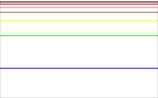
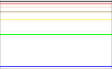
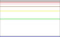
Figure 8: Eigenvalue $\lambda_{4}$ is shown for three different cases of $\tilde{\kappa}$ where different colored lines correspond $N=150$ (blue), $N=200$ (green), $N=250$ (yellow), $N=300$ (brown), $N=350$ (pink), $N=400$ (red) and $N=450$ (black)

To get a clear notion about this fact we have shown, in Figure 8, the eigenvalue $\lambda_{4}$ for three cases $\tilde{\kappa}=-0.05$, $\tilde{\kappa}=-0.1$ and $\tilde{\kappa}=-0.5$.

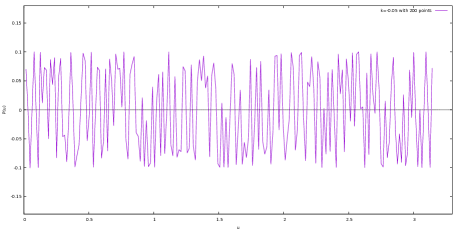
Figure 9: $P(u)$ vs $u$ plot corresponding to $\lambda_{0}$ with $\tilde{\kappa}=-0.05$ for $N=200$ points

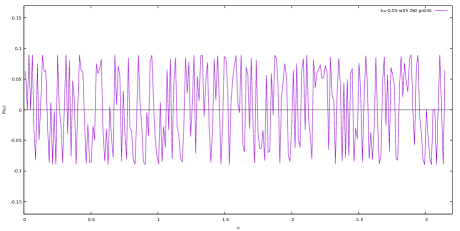
Figure 10: $P(u)$ vs $u$ plot corresponding to $\lambda_{0}$ with $\tilde{\kappa}=-0.05$ for $N=250$ points

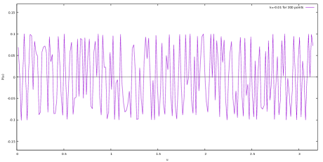
Figure 11: $P(u)$ vs $u$ plot corresponding to $\lambda_{0}$ with $\tilde{\kappa}=-0.1$ for $N=200$ points

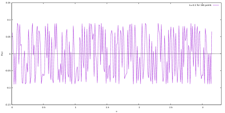
Figure 12: $P(u)$ vs $u$ plot corresponding to $\lambda_{0}$ with $\tilde{\kappa}=-0.1$ for $N=250$ points

In each of these cases we plot $\lambda_{4}$ for different number of points. Each horizontal coloured line represents $\lambda_{4}$ corresponding to $N=150,200,...$ etc. For all three cases colored lines correspond $N=150$ (blue), $N=200$ (green), $N=250$ (yellow), $N=300$ (brown), $N=350$ (pink), $N=400$ (red) and $N=450$ (black). From this plot we can now clearly understand that as we increase number of points, difference between $\lambda$ (which we have denoted as $\delta\lambda$) will decrease gradually i.e in the above diagram the blue line ($\lambda_{4}$ corresponding to $N=150$) is far apart from the green line ($\lambda_{4}$ corresponding to $N=200$). However the pink line ($N=350$) and red line ($N=400$) almost coincide and hence proves the idea of convergence. If we look at the lower eigenvalues (like $\lambda_{0}$, $\lambda_{1}$, $\lambda_{2}$, $\lambda_{3}$) we can see that the convergence is far better for them (clearly visible from table (4), (5) and (6).

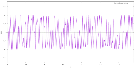
Figure 13: $P(u)$ vs $u$ plot corresponding to $\lambda_{0}$ with $\tilde{\kappa}=-0.5$ for $N=200$ points

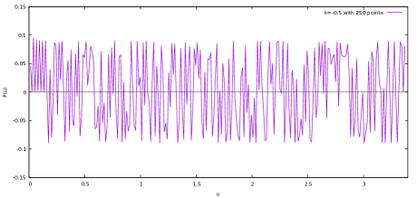
Figure 14: $P(u)$ vs $u$ plot corresponding to $\lambda_{0}$ with $\tilde{\kappa}=-0.5$ for $N=250$ points

We also show some of the solutions $P(u)$ corresponding to $\lambda_{0}$. In figures (10)-(14) plots of $P(u)$ vs $u$ for different cases are displayed. Figures (10) and (10) represent $P(u)$ vs $u$ plot for $\tilde{\kappa}=-0.05$ and for $N=200$ and $N=250$ points respectively. Similarly figures (12) and (12) are for $\tilde{\kappa}=-0.1$ and for $N=200$ and $N=250$ points respectively. So are figures (14) and (14) for $\tilde{\kappa}=-0.5$ and $N=200$ and $N=250$ points respectively. We can see clearly that all of them are oscillatory finite everywhere, with no divergences) in nature.

4.3 The full solution

In the previous section we have mainly discussed the solution of the perturbation equation (60) i.e $P(u)$. Let us now discuss the nature of $\phi(\tilde{\tau},\tilde{\sigma})$ i.e the ansatz in eqn (59). From $\phi(\tilde{\tau},\tilde{\sigma})$ we construct the normal deformations $\delta x^{i}=n_{(\alpha)}^{i}\phi^{(\alpha)}(\tilde{\tau},\tilde{\sigma})$. The normal $n^{i}$ is shown in the equation 56. Using eqn 52 and 53 we can write the normal (eqn 30) in the following form

$$\begin{split}n^{i}&=\Big{(}\frac{\sqrt{\tilde{\kappa}(1+\tilde{\kappa})}~{}{\rm cn}u}{\sqrt{-1-\tilde{\kappa}~{}{\rm cn}^{2}u+\tilde{\kappa}^{2}~{}{\rm sn}^{2}u}},-\frac{\sqrt{\tilde{\kappa}}}{\sqrt{-{\rm cn}^{2}u-\tilde{\kappa}^{2}{\rm sn}^{2}u}},\\ &~{}~{}~{}~{}~{}~{}~{}~{}\frac{{\rm cn}u}{{\rm cn}^{2}u-\tilde{\kappa}~{}{\rm sn}^{2}u}~{}\frac{\sqrt{1+\tilde{\kappa}}}{\sqrt{1+\tilde{\kappa}~{}{\rm cn}^{2}u-\tilde{\kappa}^{2}~{}{\rm sn}^{2}u}}\Big{)}\end{split}$$ (61)

The normals for three different $\kappa$ ($-0.05,~{}-0.1,~{}-0.5$) are shown in the following figures (15), (16) and (17). We can see from these plots that the normals are oscillatory in nature. We have already shown in the previous section that $P(u)$ is oscillatory in nature. To get a notion about the full solutions we need to include another quantity – $e^{i\beta\tilde{\tau}}$ which depends on the worldsheet time $\tilde{\tau}$, as shown in eqn 59. We can see from tables 1, 2 and 3 that $\lambda_{0}$ is negative for all the cases and $\lambda_{0}=\tilde{\beta}^{2}$ and $\tilde{\beta}^{2}=\frac{\beta^{2}}{1+\tilde{\kappa}}$.

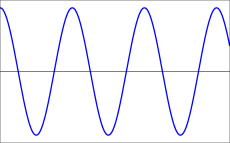
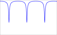
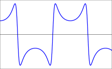
Figure 15: Three components of the normal for $\tilde{\kappa}=-0.05$

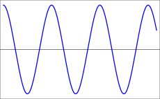
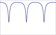
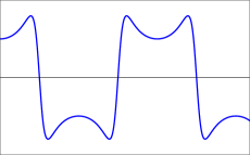
Figure 16: Three components of the normal for $\tilde{\kappa}=-0.1$

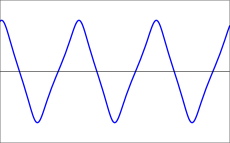
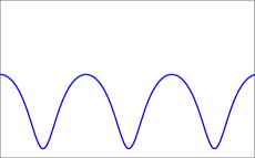
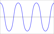
Figure 17: Three components of the normal for $\tilde{\kappa}=-0.5$

Since $1+\tilde{\kappa}$ is always positive $\beta^{2}<0$. So $\beta=\pm i\eta$ with $\eta>0$. So depending on the sign of $\beta$ we have two cases: 1) When $\beta$ is positive i.e $\beta=+i\eta$ we have the solution like $\delta x^{i}=\Big{(}\epsilon~{}P(u)~{}n^{i}\Big{)}e^{-\eta\tilde{\tau}}$ which means the perturbation will decreasing exponentially with worldsheet time $\tilde{\tau}$ and we have decaying mode. 2) When $\beta$ is negative i.e $\beta=-i\eta$ we have the solution like $\delta x^{i}=\Big{(}\epsilon~{}P(u)~{}n^{i}\Big{)}e^{\eta\tilde{\tau}}$ which means now we have a exponentially decaying perturbations with respect to worldsheet time. In these two cases $\Big{(}\epsilon~{}P(u)~{}n^{i}\Big{)}$ remains oscillatory as we have noted above.

4.4 Analytic solution

Here we develop an analytic solution of eqn 60 in a certain limit. We mainly focus on the small $\tilde{\kappa}$ limit where the potential $V(u)$ reduces to following form,

$$V(u)\equiv\frac{(1-\tilde{\kappa})(1+\tilde{\kappa}~{}{\rm sn}^{2}u)}{(1+\tilde{\kappa})(1-\tilde{\kappa}~{}{\rm sn}^{2}u)}\approx\frac{1-\tilde{\kappa}}{1+\tilde{\kappa}}\Big{(}1+2\tilde{\kappa}\sin^{2}u\Big{)}\equiv\tilde{V}(u)$$ (62)

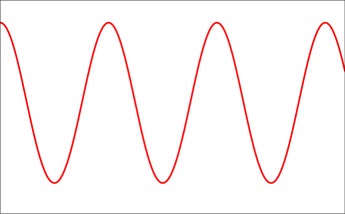
Figure 18: Plot of original potential $V(u)$ for $\tilde{\kappa}=-0.05$

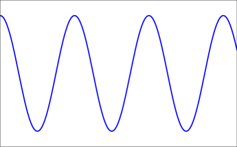
Figure 19: Plot of reduced potential $\tilde{V}(u)$ for $\tilde{\kappa}=-0.05$

We consider only the linear order terms in $\tilde{\kappa}$ and have neglected higher orders. We know at $\tilde{\kappa}=0$, ${\rm sn}~{}u=\sin u$. Thus, at very small value of $\tilde{\kappa}$ ($\tilde{\kappa}=-0.05$) ${\rm sn}~{}u$ behaves almost like a $\sin$ function i.e ${\rm sn}~{}(u,\tilde{\kappa}^{2})\equiv\sin u$. We have shown in figure (20) the original potential $V(u)$ and in figure (19) the approximated potential $\tilde{V}(u)$ for $\tilde{\kappa}=-0.05$. We can see that both of them are of identical nature which confirms the validity of our approximation. Using the approximated potential $\tilde{V}(u)$ the perturbation equation 60 will reduce to the following form,

$$\frac{d^{2}P}{du^{2}}+\Big{(}\tilde{\beta}^{2}+\frac{1-\tilde{\kappa}}{1+\tilde{\kappa}}(1+2\tilde{\kappa}\sin^{2}u)\Big{)}P=0$$ (63)

After some algebraic manipulation one can write the above equation in the following final form

$$\frac{d^{2}P}{du^{2}}+\Big{(}a-2q\cos 2u\Big{)}P=0$$ (64)

where the parameters $a$ and $2q$ are defined as

$$a=\tilde{\beta}^{2}+\frac{1-\tilde{\kappa}}{1+\tilde{\kappa}}+\frac{\tilde{\kappa}(1-\tilde{\kappa})}{1+\tilde{\kappa}}\,\,\,,\,\,\,2q=\frac{\tilde{\kappa}(1-\tilde{\kappa})}{1+\tilde{\kappa}}$$ (65)

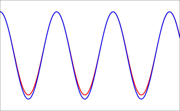
Figure 20: Plot of original potential $V(u)$ (red) with the reduced one $\tilde{V}(u)$ (blue) for $\tilde{\kappa}=-0.05$

Equation 64 is the Mathieu equation. We know the solutions of eqn 64 analytically as well as numerically. A general solution of equation 64 will be

$$P(u)=\sum_{m=0}^{\infty}\Big{(}A_{m}\cos mu+B_{m}\sin mu\Big{)}$$ (66)

with $B_{0}=0$. One can clearly see that the solution is oscillatory in nature. First few roots/characteristic values of this equation can be calculated as power series of parameter $q$

$$a_{0}(q)=-\frac{q^{2}}{2}+\frac{7q^{4}}{128}-\frac{29q^{6}}{2304}+...$$ (67)

$$a_{2}(q)=4+\frac{5q^{2}}{12}-\frac{763q^{4}}{13824}+.....$$ (68)

$$a_{4}(q)=16+\frac{q^{2}}{30}+\frac{433q^{4}}{864000}+...$$ (69)

First few eigenvalues/roots are shown in table 8. Roots almost match and both the cases follow the nature that $a_{r}\sim r^{2}$ as $q\to 0$. So, from table 8 we can say that our numerical method is appropriate and is tested here via an analytic approximation. Let us calculate $\tilde{\beta}^{2}$ from the analytical result. It turns out to be

$$\tilde{\beta}^{2}=-\frac{1-\tilde{\kappa}}{1+\tilde{\kappa}}-\frac{\tilde{\kappa}(1-\tilde{\kappa})}{1+\tilde{\kappa}}-a_{0}=-1.05038$$ (70)

Which from the numerics is $\tilde{\beta}^{2}=-1.05039$. From table 1 one can see that the corresponding value of $\tilde{\beta}^{2}=-1.05231979$. In table 8 we have shown the comparison between the analytical and numerical values for some more values of $\tilde{\beta}^{2}$. These values match quite well with the original un-approximated case of table 1. We believe this confirms the validity of the numerical results discussed in the previous section.

Table 7: Characteristic values calculated analytically and numerically

$a$	${\rm analytic~{}~{}value}$	${\rm numerical~{}~{}value}$
$a_{0}$	$-0.00038172$	$-0.000387367$
$a_{2}$	$4.00032$	$3.94217$
$a_{4}$	$16.00$	$15.0859$

Table 8: Comparison of $\tilde{\beta}^{2}$ values

$\tilde{\beta}^{2}$	${\rm analytic~{}~{}value}$	${\rm numerical~{}~{}value}$
$\tilde{\beta}^{2}_{0}$	$-1.05038$	$-1.05039$
$\tilde{\beta}^{2}_{2}$	$2.95032$	$2.89217$
$\tilde{\beta}^{2}_{4}$	$14.95$	$14.0359$

5 Concluding remarks

In this paper, first we have shown that the giant magnons in $2+1$ dimensional $\mathbb{R}\times S^{2}$ background are stable against normal perturbations. Using the Jevicki-Jin embedding we were able to reduce the perturbation equation into the wave equation in Minkowski background. The stability is demonstrated through the finite, zero mode deviations from the original profile under small deformations. We have shown this explicitly by solving the perturbation equations and by evaluating the effect of perturbations on the embedding.

Next we have studied normal deformations for single spike solutions in $\mathbb{R}\times S^{2}$. We have solved the perturbation equation numerically by using finite difference method and discussed the stability issue extensively through plots. In the end we have shown that under certain approximation the perturbation eqn reduced to the familiar Mathieu eqn. Here we have used our previous numerical method (based on the finite difference method) and have shown that the numerical result matches quite well with the analytical result. This agreement justifies the validity of the numerical results we have discussed so far. We have shown that single spike solution in this background is largely stable modulo a particular case which we have mentioned in the previous sections.

The giant magnons in $2+1$ dimensions can easily be extended to $3+1$ dimensions (i.e. for $\mathbb{R}\times S^{3}$) and hence it will be interesting to study their stability under similar normal perturbations.

A further study could be to look at the effect of the perturbations in the dual field theory side. It will be interesting to know how these perturbations are eventually related to the dual field theory operators.

Appendix A Finite difference method

Here we briefly introduce the method we have used to solve the perturbation equation (60) in the context of single spike. The finite-difference methods are a class of numerical techniques for solving differential equations by approximating derivatives with finite differences. Let us consider an interval and divide it into $n$ - sub-intervals each with size $\Delta$. According to this method one can write the quantity $\frac{d^{2}P}{du^{2}}$ in the following discretized way

$$\frac{d^{2}P}{du^{2}}=\frac{1}{\Delta^{2}}\Big{(}P(u_{i+1})-2P(u_{i})+P(u_{i-1})\Big{)}$$ (71)

where $P(u_{i})$ is the value of the function at $i$-th point. So using eqn 71 one can write eqn 60 in the following set of equations

$$\frac{1}{\Delta^{2}}\Big{(}P_{2}-2P_{1}+P_{0}\Big{)}+V_{1}P_{1} =\lambda P_{1}$$ (72)

$$\frac{1}{\Delta^{2}}\Big{(}P_{3}-2P_{2}+P_{1}\Big{)}+V_{2}P_{2} =\lambda P_{2}$$ (73)

$$\frac{1}{\Delta^{2}}\Big{(}P_{4}-2P_{3}+P_{2}\Big{)}+V_{3}P_{3} =\lambda P_{3}$$ (74)

$$\vdots$$

$$\frac{1}{\Delta^{2}}\Big{(}P_{n}-2P_{n-1}+P_{n-2}\Big{)}+V_{n-1}P_{n-1} =\lambda P_{n-1}$$ (75)

Here $P_{i}\equiv P(u_{i})$, $V_{i}\equiv V(u_{i})$ and $\lambda=-\tilde{\beta}^{2}$. Since $P(u)$ is periodic so $P_{0}=P_{n}$. Let us consider a special case of $n=4$ here. We get the following set of equations

$$\frac{1}{\Delta^{2}}\Big{(}P_{2}-2P_{1}+P_{4}\Big{)}+V_{1}P_{1} =\lambda P_{1}$$ (76)

$$\frac{1}{\Delta^{2}}\Big{(}P_{3}-2P_{2}+P_{1}\Big{)}+V_{2}P_{2} =\lambda P_{2}$$ (77)

$$\frac{1}{\Delta^{2}}\Big{(}P_{4}-2P_{3}+P_{2}\Big{)}+V_{3}P_{3} =\lambda P_{3}$$ (78)

$$\frac{1}{\Delta^{2}}\Big{(}P_{1}-2P_{4}+P_{3}\Big{)}+V_{4}P_{4} =\lambda P_{4}$$ (79)

We have used the fact $P_{0}=P_{4}$ and $P_{5}=P_{1}$ due to periodicity. Above set of equations can be written in the matrix form as follows

$$\bf M~{}P=\lambda~{}P$$ (80)

where matrix $\bf M$ is the following form

$${\bf M}=\begin{pmatrix}-\frac{2}{\Delta^{2}}+V_{1}&\frac{1}{\Delta^{2}}&0&\frac{1}{\Delta^{2}}\\ \frac{1}{\Delta^{2}}&-\frac{2}{\Delta^{2}}+V_{2}&\frac{1}{\Delta^{2}}&0\\ 0&\frac{1}{\Delta^{2}}&-\frac{2}{\Delta^{2}}+V_{3}&\frac{1}{\Delta^{2}}\\ \frac{1}{\Delta^{2}}&0&\frac{1}{\Delta^{2}}&-\frac{2}{\Delta^{2}}+V_{4}\end{pmatrix}$$ (81)

where $\bf P$ is $4\times 1$ column matrix of ${\bf P}=\Big{(}P_{0},~{}P_{1},~{}P_{2},~{}P_{3}\Big{)}$. We have considered three cases $\tilde{\kappa}=-0.05,~{}-0.1~{}\&-0.5$ and compute the eigenvalues ($\lambda$) and eigenfunctions (${\bf P}$) for certain number of points ($150,~{}200,~{}250$) for each cases in section 4.2.

References

- (1) C. J. Burden and L. J. Tassie, “Some exotic mesons and glueballs from the string model,” Phys. Letts. B 110, 64 (1982).
- (2) C. J. Burden and L. J. Tassie, “Rotating strings, glueballs and exotic mesons,” Aust. Jr. Phys. 35, 223 (1982).
- (3) C. J. Burden and L. J. Tassie, “ Additional rigidly rotating solutions in the string model of hadrons,” Aust. Jr. Phys. 37, 1 (1984).
- (4) C. J. Burden, “Gravitational radiation from a particular class of cosmic strings,” Phys. Letts. B, 164, 277 (1985).
- (5) F. Embacher, “Rigidly rotating cosmic strings,” Phys. Rev. D 46, 3659 (1992); Erratum Phys. Rev. D 47, 4803 (1993).
- (6) H. de Vega and I. L. Egusquiza, “ Planetoid string solutions in axisymmetric spacetimes”, Phys. Rev. D 54, 7513 (1996) [arXiv:hep-th/9607056].
- (7) V. Frolov, S. Hendy and J. P. de Villiers, “ Rigidly rotating strings in stationary axisymmetric spacetimes”, Class. Qtm. Grav. 14, 1099 (1997) [arXiv:hep-th/9612199].
- (8) S. Kar and S. Mahapatra, “ Planetoid strings: solutions and perturbations”, Class. Qtm. Grav. 15, 1421 (1998) [arXiv:hep-th/9701173].
- (9) C. J. Burden, “Comment on “Stationary rotating strings as relativistic particle mechanics”,” Phys. Rev. D 78, 128301 (2008).
- (10) K. Ogawa, H. Ishihara, H. Kozaki, H. Nakano and S. Saito, “ Stationary rotating strings as relativistic particle mechanics ”, Phys. Rev. D 78, 023525 (2008) [arXiv:gr-qc/0803.4072].
- (11) J. M. Maldacena, “The Large N limit of superconformal field theories and supergravity,” Int. J. Theor. Phys. 38, 1113 (1999) [Adv. Theor. Math. Phys. 2, 231 (1998)] [hep-th/9711200].
- (12) M. Kruczenski, “Spiky strings and single trace operators in gauge theories,” JHEP 0508, 014 (2005) [arXiv:hep-th/0410226].
- (13) S. S. Gubser, I. R. Klebanov and A. M. Polyakov, Nucl. Phys. B 636, 99 (2002) [hep-th/0204051].
- (14) J. A. Minahan and K. Zarembo, “The Bethe ansatz for =4 super Yang-Mills,” JHEP 0303, 013 (2003) [hep-th/0212208].
- (15) L. Dolan, C. R. Nappi and E. Witten, “A Relation between approaches to integrability in superconformal Yang-Mills theory,” JHEP 0310, 017 (2003) [arXiv:hep-th/0308089].
- (16) L. Dolan, C. R. Nappi and E. Witten, “Yangian symmetry in superconformal Yang-Mills theory,” [arXiv:hep-th/0401243]
- (17) G. Mandal, N. V. Suryanarayana and S. R. Wadia, “Aspects of semiclassical strings in AdS(5),” Phys. Lett. B 543, 81 (2002) [hep-th/0206103].
- (18) I. Bena, J. Polchinski and R. Roiban, “Hidden symmetries of the AdS(5) x S**5 superstring,” Phys. Rev. D 69, 046002 (2004) [hep-th/0305116].
- (19) D. M. Hofman, J. M. Maldacena, “Giant Magnons,” J. Phys. A39, 13095, (2006).
- (20) S. Frolov and A. A. Tseytlin, “Multispin string solutions in AdS(5) x S**5,” Nucl. Phys. B 668, 77 (2003) [hep-th/0304255].
- (21) N. Dorey, “Magnon bound states and the AdS/CFT correspondence,” J. Phys., A39, 13119-13128, doi:10.1088/0305-4470/39/41/S18.
- (22) H. Y. Chen, N. Dorey, K. Okamura, “Dyonic giant magnons,” JHEP, 09, 024, doi:10.1088/1126-6708/2006/09/024.
- (23) H. Y. Chen, N. Dorey, K. Okamura, “On the scattering of magnon bound states,” JHEP, 11, 035, doi:10.1088/1126-6708/2006/11/035.
- (24) M. Kruczenski, J. Russo, A. A. Tseytlin, “Spiky strings and giant magnons on ,” JHEP, 10, 002, doi:10.1088/1126-6708/2006/10/002.
- (25) S. Hirano, “Fat magnon,” JHEP, 04, 010, doi:10.1088/1126-6708/2007/04/010.
- (26) D. M. Hofman, J. M. Maldacena, “Reflecting magnons,” JHEP, 11, 063. doi:10.1088/1126-6708/2007/11/063.
- (27) J. M. Maldacena, I. Swanson, “Connecting giant magnons to the pp-wave: An interpolating limit of .” Phys. Rev., D76, 026002. doi:10.1103/PhysRevD.76.026002.
- (28) R. Ishizeki and M. Kruczenski, “Single spike solutions for strings on and ,” Phys. Rev. D 76, 126006 (2007) [arXiv:0705.2429 [hep-th]].
- (29) G. Arutyunov, S. Frolov, M. Zamaklar, “Finite-size effects from giant magnons,” Nucl.Phys., B778, 1-35, doi:10.1016/j.nuclphysb.2006.12.026.
- (30) N. Dorey, K. Okamura, “Singularities of the magnon boundstate S-Matrix,” JHEP, 03, 037. doi:10.1088/1126-6708/2008/03/037.
- (31) R. Ishizeki, M. Kruczenski, A. Tirziu and A. A. Tseytlin, “Spiky strings in and their AdS-pp-wave limits,” Phys. Rev. D 79, 026006 (2009) [arXiv:0812.2431 [hep-th]].
- (32) S. Biswas and K. L. Panigrahi, “Spiky Strings on I-brane,” JHEP 1208, 044 (2012) [arXiv:1206.2539 [hep-th]].
- (33) A. Banerjee, K. L. Panigrahi and P. M. Pradhan, “Spiky strings on with NS-NS flux,” Phys. Rev. D 90, no. 10, 106006 (2014) [arXiv:1405.5497 [hep-th]].
- (34) A. Banerjee, S. Bhattacharya and K. L. Panigrahi, “Spiky strings in -deformed ,” JHEP 1506, 057 (2015) [arXiv:1503.07447 [hep-th]].
- (35) S. Bhattacharya, S. Kar and K. L. Panigrahi, “Perturbations of spiky strings in flat spacetimes”, JHEP 01, 116 (2017) [arXiv:hep-th/1610.09180].
- (36) S. Bhattacharya, S. Kar and K. L. Panigrahi, “Perturbations of spiky strings in , JHEP 06, 089 (2018) [arXiv:hep-th/1804.07544].
- (37) J. Garriga and A. Vilenkin, “Black holes from nucleating strings,” Phys. Rev. D 47 3265 (1993) [arXiv:hep-ph/9208212].
- (38) J. Guven, “Perturbations of a topological defect as a theory of coupled scalar fields in curved space interacting with an external vector potential,” Phys. Rev. D 48, 5562 (1993) [arXiv:gr-qc/9304033].
- (39) V. Frolov and A. L. Larsen, “Propagation of perturbations along strings”, Nucl. Phys. B 414, 129 (1994) [arXiv:hep-th/9303001].
- (40) R. Capovilla and J. Guven, “Geometry of deformations of relativistic membranes,” Phys. Rev. D 51, 6736 (1995) [arXiv:gr-qc/9411060].
- (41) S. Frolov and A. A. Tseytlin, “Semiclassical quantization of rotating superstring in AdS(5) x S**5,” JHEP 0206, 007 (2002) [hep-th/0204226].
- (42) V. Forini, V. Giangreco, M. Puletti, L. Griguolo, D. Seminara, E. Vescovi, “Remarks on the geometrical properties of semiclassically quantized strings”, J. Phys A: Math. Theor., 48, 475401 (2015) [arXiv:1507.01883 [hep-th]].
- (43) E. Rojas, “Covariant perturbations in the gonihedric string model”, Int. J. Mod. Phys., A32(32), 1750192.
- (44) M. Hasegawa and D. Ida, “Instability of stationary closed strings winding around flat torus in five-dimensional Schwarzschild spacetimes”, Phys. Rev. D98(4).
- (45) S. P. Barik, K. L. Panigrahi, “Purturbations of Pulsating strings”, arXiv:1708.05202[hep-th].
- (46) A. Jevicki and K. Jin, “Solitons and AdS string solutions”, Int. Jr. Mod. Phys. A 23, 2289 (2008) [arXiv:0804.0412 [hep-th]].
- (47) Y-M. Chiang, A. Ching and C-Y. Tsang, “Symmetries of the Darboux equation”, [arXiv:1509.03995 [math]] (to appear in Kumamoto Journal of Mathematics).