Fast Newton method solving KLR based on Multilevel Circulant Matrix with log-linear complexity

Abstract

Kernel logistic regression (KLR) is a conventional nonlinear classifier in machine learning. With the explosive growth of data size, the storage and computation of large dense kernel matrices is a major challenge in scaling KLR. Even the nyström approximation is applied to solve KLR, it also faces the time complexity of $O(nc^{2})$ and the space complexity of $O(nc)$, where $n$ is the number of training instances and $c$ is the sampling size. In this paper, we propose a fast Newton method efficiently solving large-scale KLR problems by exploiting the storage and computing advantages of multilevel circulant matrix (MCM). Specifically, by approximating the kernel matrix with an MCM, the storage space is reduced to $O(n)$, and further approximating the coefficient matrix of the Newton equation as MCM, the computational complexity of Newton iteration is reduced to $O(n\log n)$. The proposed method can run in log-linear time complexity per iteration, because the multiplication of MCM (or its inverse) and vector can be implemented the multidimensional fast Fourier transform (mFFT). Experimental results on some large-scale binary-classification and multi-classification problems show that the proposed method enables KLR to scale to large scale problems with less memory consumption and less training time without sacrificing test accuracy.

1 Introduction

Kernel logistic regression (KLR) is a log-linear model with direct probabilistic interpretation and can be naturally extended to multi-class classification problems [jaakkola1999probabilistic]. It is widely used in many fields, including automatic disease diagnosis [choudhury2021predicting], detecting fraud [TJLT201908008], landslide susceptibility mapping [hong2015spatial], etc. But it is difficult to scale to large-scale problems due to its high space and time complexity. A key issue in extending KLR to large-scale problems is the storage and computation of the kernel matrix, which is usually intensive. In particular, when Newton method is used to solve KLR, the inverse operation of the Hessian matrix in each iteration requires $O(n^{3})$ time and requires $O(n^{2})$ space to store the kernel matrix.

A number of researchers have been working to make KLR feasible for large-scale problems [zhu2005kernel, sugiyama2010computationally, keerthi2005fast]. They mainly start from the following two aspects: sparsity of solutions or decomposing the original problem into subproblems. Inspired by the sparsity of support vector machine (SVM), Zhu and Hastie [zhu2005kernel] proposed the import vector machine (IVM) algorithm to reduced the time complexity of the binary classification of KLR to $O(n^{2}s^{2})$, where $s$ is the number of import points. IVM is still difficult to calculate for large-scale problems although the complexity has been reduced. Inspired by sequence minimum optimization algorithm (SMO) solving SVM, Keerthi et al. [keerthi2005fast] proposed a fast dual algorithm for solving KLR. By continuously decomposing the original problem into subproblems, the fast dual algorithm only updates two variables per iteration. However, the time cost of iteratively updating values in the fast dual algorithm is increased by the introduction of the kernel matrix calculation. In short, existing methods still make it difficult to scale KLR to large-scale problems.

In this paper, we focus on kernel approximation to accelerate large-scale KLR inspired by the excellent performance of kernel approximation in learning problems [NIPS2000_19de10ad, lei2020improved, jia2020large, chen2021fast]. A great deal of work has been done on kernel approximation. The commonly used kernel approximation methods include Nyström method [li2014large, calandriello2016analysis, NIPS2015_f3f27a32, NIPS2017_a03fa308, kumar2012sampling, gittens2016revisiting], random feature [NIPS2007_013a006f, he2019fast, pmlr-v28-le13, feng2015random, xiong8959408kui, dao2017gaussian, munkhoeva2018quadrature, Zhuli2021towards, liu2020random], multilevel circulant matrix (MCM) [song2009approximation, song2010approximation, ding2011approximate, edwards2013approximate, ding2017approximate, ding2020approximate], and so on.

Nyström method is the classical kernel matrix approximation, whose outstanding feature is the sampling of data before large-scale matrix operations. After the Nyström method successfully and efficiently solves large-scale Gaussian processes [NIPS2000_19de10ad], a number of sampling methods with strong theoretical guarantees have been proposed to satisfy the desired approximation with fewer sampling points. Among these sampling methods, the leverage score sampling technique [NIPS2015_f3f27a32] is the most widely used in practical applications. Recursive ridge leverage scores (RRLS) [NIPS2017_a03fa308] finds a more accurate kernel approximation in less time by employing a fast recursive sampling scheme. However, in [yin2019sketch] the authors pointed out that the Nyström approximation is very sensitive to inhomogeneities in the sample.

The random feature is constructed randomly from a nonlinear mapping of the input space to the Hilbert space, that is, the direct approximation of the kernel function without calculating the elements in the kernel matrix. Rahimi and Recht [NIPS2007_013a006f] proposed the random feature map of shifted invariant kernel functions based on Fourier transform. In order to speed up feature projection, Feng et al. [feng2015random] proposed structured random matrices, signed Circulant Random Matrix (CRM), to project input data. The feature mapping can be done in $O(nD\log d)$ time by using the fast Fourier Transform (FFT), where $d$ and $D$ represent the dimensions of the input data and the random feature space, respectively. Li et al. [Zhuli2021towards] provided the first unified risk analysis of learning with random Fourier features and proposed leverage score random feature mapping which needs $O(nD^{2}+D^{3})$ time to generate refined random features. Obviously, when $d$ or $D$ is very large, the feature mapping is costly.

The idea of MCM approximate kernel matrix was first proposed by Song and Xu [song2010approximation] and many theoretical results are proven. By approximated the kernel matrix with MCM, researchers have developed many applications in different machine learning areas, such as the kernel ridge regression [edwards2013approximate], automatic kernel selection problem [ding2017approximate] and least squares support vector machines [ding2020approximate], where the approximated kernel matrix is stored in $O(n)$ and the computational complexity of the corresponding algorithms is only $O(n\log n)$. Since MCM can save a lot of memory and has certain computing advantages, we choose MCM approximation to speed up KLR.

In the works [edwards2013approximate, ding2017approximate, ding2020approximate], the core problem is to solve a system of linear equations $(\boldsymbol{K}+n\lambda\boldsymbol{I}){\boldsymbol{d}}={\boldsymbol{b}}$, where $\boldsymbol{K}$ is a kernel matrix or the linear combination of multiple kernel matrices and $\lambda$ is the regularized parameter. If $\boldsymbol{K}$ is approximated by an MCM, then $(\boldsymbol{K}+n\lambda\boldsymbol{I})$ is MCM too, hence the system of linear equations can be solved in $O(n\log n)$ time by the multidimensional fast Fourier transform (mFFT) owing to the advantages of MCM. When applying MCM directly to KLR, it faces to solve a system of linear equations $\left({\boldsymbol{K}}^{\top}\boldsymbol{\Lambda}\boldsymbol{K}+n\lambda\boldsymbol{K}\right)\boldsymbol{d}=\boldsymbol{b}.$ Only approximated $\boldsymbol{K}$ as an MCM, the coefficient matrix of the system of linear equations is still not an MCM. Hence it cannot be solved in $O(n\log n)$ and still suffers from high computational complexity. In this case, the most efficient scheme to solve it is to run conjugate gradient method $T$ loops with the computational complexity $O(Tn\log n)$. Since $T=O(n)$ for conjugate gradient method [hestenes1952methods], this scheme is still insufferable for large-scale problems.

In this work, to effectively solve KLR with large-scale training samples, we firstly simplify the resulted Newton equation, then approximate the kernel matrix by MCM as [edwards2013approximate, ding2017approximate, ding2020approximate] did. Further we approximate the coefficient matrix of the simplified Newton equation as an MCM too. Hence, we propose a fast Newton method based on MCM which can efficient solve large-scale KLR with $O(n)$ space complexity and $O(n\log n)$ computational complexity. Many experimental results support that the proposed method can make KLR problem scalable.

The rest of the paper is organized as follows. In Section 2, we review KLR and MCM. In Section 3, we present the fast Newton method based on MCM approximation for solving KLR. We report experimental results in Section LABEL:section:4. Section LABEL:section:5 concludes this paper.

2 Preliminaries

In this section, we review KLR and MCM and introduce some interesting properties of MCM.

2.1 Kernel Logistic Regression

Given the training set $\mathbb{D}=\{(\boldsymbol{x}_{i},\boldsymbol{y}_{i}),i=1,\ldots,n\}$, where $\boldsymbol{x}_{i}\in\mathcal{X}\in\mathbb{R}^{d}$ is the input data and $\boldsymbol{y}_{i}\in\{0,1\}$ is the output targets corresponding to the input. A reproducing kernel Hibert space $\mathbb{H}$ is defined by a kernel function $\kappa(\boldsymbol{x},\boldsymbol{z})=\left<\varphi(\boldsymbol{x}),\varphi(\boldsymbol{z})\right>$ with $\varphi:\mathbb{R}^{d}\mapsto\mathbb{H}$, which measures the inner product between the input vectors in the feature space. Then a traditional logistic regression model [cawley2004efficient] is constructed in the feature space as follows

$$\min_{\boldsymbol{w}\in\mathbb{H}}\frac{\lambda}{2}{\|\boldsymbol{w}\|}^{2}-\frac{1}{n}(\boldsymbol{y}^{\top}\ln\boldsymbol{p}+(\boldsymbol{1}-\boldsymbol{y})^{\top}\ln(\boldsymbol{1}-\boldsymbol{p})),$$ (1)

where $\boldsymbol{p}_{i}=1/(1+e^{-\left<\boldsymbol{w},\varphi(\boldsymbol{x}_{i})\right>})$ is the posterior probability estimation of $\boldsymbol{y}_{i}=1$, $\lambda>0$ is the regularization parameter, and $\boldsymbol{1}$ is the all-one vector.

By the representer theorem [scholkopf2001generalized], the solution to the optimization problem (1) can be represented as

$$\boldsymbol{w}=\sum_{i=1}^{n}\boldsymbol{\alpha}_{i}\varphi\left(\boldsymbol{x}_{i}\right),$$ (2)

where $\boldsymbol{\alpha}\in\mathbb{R}^{n}$. Then plugging (2) in (1), we can get the following KLR model

$$\mathop{\min}\limits_{\boldsymbol{\alpha}\!\in{\mathbb{R}^{n}}}\!F(\boldsymbol{\alpha})\!=\!\frac{\lambda}{2}{\boldsymbol{\alpha}\!^{\top}}\boldsymbol{K}\!\boldsymbol{\alpha}\!-\!\frac{1}{n}({\boldsymbol{y}\!^{\top}}\!\ln\boldsymbol{p}\!+\!{{(\boldsymbol{1}\!-\!\boldsymbol{y})}\!^{\top}}\!\ln(\boldsymbol{1}\!-\!\boldsymbol{p})),$$ (3)

where $\boldsymbol{K}$ is the kernel matrix satisfying $\boldsymbol{K}_{i,j}=\kappa(\boldsymbol{x}_{i},\boldsymbol{x}_{j})$, ${\boldsymbol{p}}_{i}=1/({{1+{e^{-\boldsymbol{K}(i,\cdot)\boldsymbol{\alpha}}}}})$, and $\boldsymbol{K}(i,\cdot)$ denotes the $i$-th row of the kernel matrix.

KLR is a convex optimization problem, which can be solved by Newton method [dennis1996numerical] with quadratic convergence rate. However, Newton method requires $O(n^{3})$ time complexity and $O(n^{2})$ space complexity for each iteration, which is not feasible for large-scale data sets. Therefore, we need a more effective method to solve KLR.

2.2 Multilevel Circulant Matrix Approximation

Here we introduce the concept of MCM and some of its interesting properties, and analyze its computational advantages.

To facilitate representation, we introduce the notion of multilevel indexing [song2010approximation]. In order to construct a $q$-level circulant matrix of level order $\boldsymbol{q}$, it is necessary to decompose $n\in\mathbb{N}$ into the product of $q\in\mathbb{N}$ positive integers, that is, $n=n_{0}n_{1}\cdots n_{q-1}$. We denote $\boldsymbol{q}:=\left[n_{0},n_{1},\ldots,n_{q-1}\right]\in\mathbb{N}^{q}$. Then, multilevel indexing $[\boldsymbol{q}]$ of the $q$-level circulant matrix is defined as follows

$$[\boldsymbol{q}]\!:=\!\left[n_{0}\right]\!\times\!\left[n_{1}\right]\!\times\!\cdots\!\times\![n_{q-1}]\!\in\mathbb{R}^{n\times q}\!,$$ (Cartesian product)

where $[n_{q-j}]:=\{0,1,\ldots,n_{q-j}\},j=1,2,\ldots,q$.

According to [tyrtyshnikov1996unifying], if a matrix $\boldsymbol{K}_{\boldsymbol{q}}$ consists of $n_{0}\times n_{0}$ blocks and each block $(q-1)$-level circulant matrix of level order $[n_{1},\ldots,n_{q-1}]$, then $\boldsymbol{K}_{\boldsymbol{q}}$ is called a $q$-level circulant matrix. In other words, an MCM is a matrix that can be partitioned into blocks, which are further partitioned into smaller blocks. Specifically, $\boldsymbol{K}_{\boldsymbol{q}}=[\boldsymbol{K}_{\boldsymbol{i},\boldsymbol{j}}:\boldsymbol{i},\boldsymbol{j}\in[\boldsymbol{q}]]$ is called a $q$-level circulant matrix if for any $\boldsymbol{i}=({\boldsymbol{i}}_{0},{\boldsymbol{i}}_{1},\ldots,{\boldsymbol{i}}_{q-1})\in[\boldsymbol{q}]$, $\boldsymbol{j}=({\boldsymbol{j}}_{0},{\boldsymbol{j}}_{1},\ldots,{\boldsymbol{j}}_{q-1})\in[\boldsymbol{q}]$,

$$\boldsymbol{K}_{\boldsymbol{i},\boldsymbol{j}}=\boldsymbol{k}_{{\boldsymbol{i}}_{0}-\bmod\left({\boldsymbol{j}}_{0},n_{0}\right),\ldots,{\boldsymbol{i}}_{q-1}-\bmod({\boldsymbol{j}}_{q-1},n_{q-1})},$$

where $\boldsymbol{k}$ is the first column of $\boldsymbol{K}_{\boldsymbol{q}}$. Then a $q$-level circulant matrix $\boldsymbol{K}_{\boldsymbol{q}}$ is fully determined by its first column. So we write ${\boldsymbol{K}_{\boldsymbol{q}}}={circ_{\boldsymbol{q}}}[{\boldsymbol{k}}]$.

The computational advantages of MCM are analyzed in detail in [davis1979circulant], and the key conclusions are restated as follows.

Lemma 1.

[davis1979circulant] Suppose that $\boldsymbol{K}_{\boldsymbol{q}}$ is an MCM of level order $\boldsymbol{q}$ and $\boldsymbol{k}$ is its first column. Then $\boldsymbol{K}_{\boldsymbol{q}}$ is a $q$-level circulant matrix of level order $\boldsymbol{q}$ if and only if

$$\boldsymbol{K}_{\boldsymbol{q}}=\frac{1}{n}\boldsymbol{\phi}^{*}\operatorname{diag}(\boldsymbol{\phi}\boldsymbol{k})\boldsymbol{\phi},$$ (4)

where $\boldsymbol{\phi}=\boldsymbol{F}_{n_{0}}\otimes\boldsymbol{F}_{n_{1}}\otimes\cdots\otimes\boldsymbol{F}_{n_{q-1}}$, $\boldsymbol{A}\otimes\boldsymbol{B}$ denotes the Kronecker product of $\boldsymbol{A}$ and $\boldsymbol{B}$, and $\boldsymbol{F}_{n_{q-j}}=[e^{(2\pi i/n_{q-j})st}:s,t\in[n_{q-j}]]$, $j=1,2,\ldots,q$ with $i$ being the imaginary unit.

Theorem 1.

[davis1979circulant] Assume that $\boldsymbol{A}_{\boldsymbol{q}}$ and $\boldsymbol{B}_{\boldsymbol{q}}$ are both MCM of level order $\boldsymbol{q}$, then $\boldsymbol{A}_{\boldsymbol{q}}+\boldsymbol{B}_{\boldsymbol{q}}$ is also an MCM of level order $\boldsymbol{q}$.

Theorem 2.

[davis1979circulant] Assume that $\boldsymbol{A}_{\boldsymbol{q}}$ is an invertible MCM of level order $\boldsymbol{q}$ and $\boldsymbol{a}$ is the first column of $\boldsymbol{A}_{\boldsymbol{q}}$, $\boldsymbol{\nu}=\boldsymbol{\phi}\boldsymbol{a}$ is the vector of eigenvalues, then $\boldsymbol{A}_{\boldsymbol{q}}^{-1}$ is also an MCM, and $\boldsymbol{A}_{\boldsymbol{q}}^{-1}=(1/n)\boldsymbol{\phi}^{*}(\operatorname{diag}({\boldsymbol{\nu}}))^{-1}\boldsymbol{\phi}$.

The following Algorithm 1 proposed in [song2009approximation] can construct an MCM $\boldsymbol{K}_{\boldsymbol{q}}$ from a kernel function to approximate the kernel matrix $\boldsymbol{K}$.

Algorithm 1 Construction of an MCM [song2009approximation]

1:a kernel function $\kappa$, a sequence of positive numbers $\boldsymbol{h}=({\boldsymbol{h}_{0}},{\boldsymbol{h}_{1}},\ldots,{\boldsymbol{h}_{q-1}})\in{\mathbb{R}^{q}}$, level order $\boldsymbol{q}\in{\mathbb{N}^{q}}$.

2:$\boldsymbol{K}_{\boldsymbol{q}}$.

3:Calculate ${\boldsymbol{t}_{\boldsymbol{i}}}=\kappa\left({\|[{{{\boldsymbol{i}}_{s}}{{\boldsymbol{h}}_{s}}:s\in[q]}]\|_{2}}\right)$, $\forall\boldsymbol{i}\in[\boldsymbol{q}]$.

4:Let ${\boldsymbol{D}_{\boldsymbol{i},s}}=\left\{{\begin{array}[]{*{20}{c}}{\{0\},}\\ {\{{\boldsymbol{i}_{s}},{\boldsymbol{q}_{s}}-{\boldsymbol{i}_{s}}\},}\\ \end{array}}\right.\begin{array}[]{*{20}{c}}{{\boldsymbol{i}_{s}}=0,}\\ {1\leqslant{\boldsymbol{i}_{s}}\leqslant{\boldsymbol{q}_{s}}-1,}\\ \end{array}$ and ${\boldsymbol{D}_{\boldsymbol{i}}}={\boldsymbol{D}_{\boldsymbol{i},0}}\times{\boldsymbol{D}_{\boldsymbol{i},1}}\times\cdots\times{\boldsymbol{D}_{\boldsymbol{i},q-1}}$, $\forall\boldsymbol{i}\in[\boldsymbol{q}]$ and $\forall s\in[q]$.

5:Calculate $\boldsymbol{k}_{\boldsymbol{i}}=\sum\limits_{\boldsymbol{j}\in{\boldsymbol{D}_{\boldsymbol{i}}}}{\boldsymbol{t}_{\boldsymbol{j}}}$.

6:return $\boldsymbol{K}_{\boldsymbol{q}}=circ_{\boldsymbol{q}}[\boldsymbol{k}]$.

For $\boldsymbol{K}_{\boldsymbol{q}}$ generated by Algorithm 1, only $O(n)$ is required to store it since we only need to store the first column. By Lemma 1, $\boldsymbol{K}_{\boldsymbol{q}}\boldsymbol{x}$ is equivalent to implementing $(1/n)\boldsymbol{\phi}^{*}\operatorname{diag}(\boldsymbol{\phi}\boldsymbol{k})\boldsymbol{\phi}\boldsymbol{x}$, which can be realized efficiently in $O(n\log n)$ using the mFFT. According to Theorem 2, ${\boldsymbol{K}_{\boldsymbol{q}}^{-1}}\boldsymbol{x}$ is equivalent to implementing $(1/n)\boldsymbol{\phi}^{*}(\operatorname{diag}(\boldsymbol{\phi}\boldsymbol{k}))^{-1}\boldsymbol{\phi}\boldsymbol{x}$, which also can be realized efficiently in $O(n\log n)$. In addition to its advantages in computation and space storage, MCM approximation also does not require any sampling techniques. Next, we will design a fast and effective method to solve KLR based on MCM.

3 Fast Newton Method Based on MCM Approximation

In this section, we first simplify the Newton equation of KLR, then approximate the coefficient matrix of the simplified Newton equation as an MCM, finally propose a fast Newton method based on MCM approximation.

3.1 Simplify the Newton equation

KLR is a convex optimization problem [boyd2004convex], and the local optimal solution must be the global optimal solution. For convex optimization issues, Newton method with at least quadratic convergence can be used to solve them. The gradient and Hessian are obtained by differentiating (3) with respect to $\boldsymbol{\alpha}$. The gradient is

$$\nabla F(\boldsymbol{\alpha})=\lambda\boldsymbol{K}\boldsymbol{\alpha}-\frac{1}{n}{\boldsymbol{K}}(\boldsymbol{y}-\boldsymbol{p}),$$ (5)

and the Hessian of (3) is

$${\nabla^{2}}F(\boldsymbol{\alpha})=\frac{1}{n}{\boldsymbol{K}^{\top}}\boldsymbol{\Lambda}\boldsymbol{K}+\lambda\boldsymbol{K},$$ (6)

where $\boldsymbol{\Lambda}$ is a diagonal matrix with $\boldsymbol{\Lambda}_{ii}={\boldsymbol{p}_{i}}(1-{\boldsymbol{p}_{i}})$. Based on the (5) and (6), we need to solve the following Newton equation

$$\left({\boldsymbol{K}^{\top}}\boldsymbol{\Lambda}\boldsymbol{K}+n\lambda\boldsymbol{K}\right){\boldsymbol{d}}={\boldsymbol{K}}(\boldsymbol{y}-\boldsymbol{p}-n\lambda\boldsymbol{\alpha}),$$ (7)

to update the current solution. Obviously, in order to compute the Newton direction $\boldsymbol{d}$, the computational complexity is $O({n^{3}})$ per iteration, which is prohibitively expensive for large-scale problems. In order to reduce the computational cost, we first simplify the Newton equation. Since the kernel matrix is symmetric, we have

$$\boldsymbol{K}(\boldsymbol{\Lambda}\boldsymbol{K}+n\lambda\boldsymbol{I}){\boldsymbol{d}}=\boldsymbol{K}(\boldsymbol{y}-\boldsymbol{p}-n\lambda\boldsymbol{\alpha}).$$ (8)

If the kernel matrix $K$ is positive definite, we can simplify (8) as

$$(\boldsymbol{\Lambda}\boldsymbol{K}+n\lambda\boldsymbol{I}){\boldsymbol{d}}=\boldsymbol{y}-\boldsymbol{p}-n\lambda\boldsymbol{\alpha}.$$ (9)

If the kernel matrix $\boldsymbol{K}$ is positive semidefinite, then the solution to (8) is not necessarily unique, but the unique solution of (9) is the solution of (8). Therefore, we can use the solution of (9) as the Newton direction.

Replacing $\boldsymbol{K}$ in (9) with $\boldsymbol{K}_{\boldsymbol{q}}$ generated by Algorithm 1, we can further obtain the following approximated Newton equation

$$(\boldsymbol{\Lambda}\boldsymbol{K}_{\boldsymbol{q}}+n\lambda\boldsymbol{I}){\bar{\boldsymbol{d}}}=\boldsymbol{y}-\bar{\boldsymbol{p}}-n\lambda\boldsymbol{\alpha},$$ (10)

where $\bar{\boldsymbol{p}}_{i}=1/({{1+{e^{-\boldsymbol{K}_{\boldsymbol{q}}(i,\cdot)\boldsymbol{\alpha}}}}}$) and $\boldsymbol{K}_{\boldsymbol{q}}(i,\cdot)$ is the $i$-th row of $\boldsymbol{K}_{\boldsymbol{q}}$.

If solving (10) by the conjugate gradient method [hestenes1952methods] to obtain an approximated Newton direction, the time complexity of each iteration is $O(n\log n)$ due to the use of mFFT.

In this case, the most efficient scheme to solve (10) is to run conjugate gradient method $T$ loops with the computational complexity $O(Tn\log n)$. Since $T=O(n)$ for conjugate gradient method [hestenes1952methods], this scheme is still insufferable for large-scale problems. Then we expect to find a more efficient way to calculate the Newton direction.

3.2 Approximate the Coefficient Matrix of Newton Equation using MCM

In this section, we approximate the coefficient matrix of equation (10) as an MCM, then we can calculate the Newton direction more efficiently.

According to Theorem 2, if we can approximate $\boldsymbol{\Lambda}\boldsymbol{K}_{\boldsymbol{q}}+n\lambda\boldsymbol{I}$ with an MCM, then we can directly calculate ${\bar{\boldsymbol{d}}}$ in $O(n\log n)$ time by using mFFT. Obviously, we only need to approximate $\boldsymbol{\Lambda}\boldsymbol{K}_{\boldsymbol{q}}$ since $n\lambda\boldsymbol{I}$ is already an MCM. To this end, we solve the least squared problem

$$\min_{\boldsymbol{A}_{\boldsymbol{q}}\in\mathbb{A}_{\boldsymbol{q}}}\quad\|\boldsymbol{\Lambda}\boldsymbol{K}_{\boldsymbol{q}}-\boldsymbol{A}_{\boldsymbol{q}}\|_{F}^{2},$$ (11)

where $\mathbb{A}_{\boldsymbol{q}}$ is the set of MCM of level order $\boldsymbol{q}$. Here we use the Frobenius Norm for simplicity, and the other norms of matrix can be used.

By working out the optimality condition of the problem (11), we obtain the following proposition.

Proposition 1.

The optimal solution of the problem (11) is

$$\boldsymbol{A}_{\boldsymbol{q}}=\tau\boldsymbol{K}_{\boldsymbol{q}},$$ (12)

where $\tau=(1/n)\sum_{i=1}^{n}{\boldsymbol{\Lambda}_{ii}}$.

Proof: Let $\boldsymbol{k}$ be the first column of $\boldsymbol{K}_{\boldsymbol{q}}$ and $\boldsymbol{a}$ be the first column of $\boldsymbol{A}_{\boldsymbol{q}}$, where $\boldsymbol{k}=(\boldsymbol{k}_{1},\boldsymbol{k}_{2},\ldots,\boldsymbol{k}_{n})$ and $\boldsymbol{a}=(\boldsymbol{a}_{1},\boldsymbol{a}_{2},\ldots,\boldsymbol{a}_{n})$. According to the built-in periodicity of $\boldsymbol{K}_{\boldsymbol{q}}$ and $\boldsymbol{A}_{\boldsymbol{q}}$, the problem (11) is equivalent to

$$\min_{a_{j}\in\mathbb{R}}\quad\sum_{i=1}^{n}\sum_{j=1}^{n}{(\boldsymbol{\Lambda}_{ii}\boldsymbol{k}_{j}-\boldsymbol{a}_{j})^{2}}.$$ (13)

The first-order optimality conditions of the problem (13) is

$$\sum_{i=1}^{n}{(\boldsymbol{\Lambda}_{ii}\boldsymbol{k}_{j}-\boldsymbol{a}_{j})}=0,j=1,2,\ldots,n.$$

Hence, the optimal solution of the problem (13) is

$$\boldsymbol{a}_{j}=\frac{1}{n}\sum_{i=1}^{n}{\boldsymbol{\Lambda}_{ii}}\boldsymbol{k}_{j},j=1,2,\ldots,n.$$

Thus the optimal solution of the problem (11) is (12), which proves the proposition.

According to Proposition 1, we replace $\boldsymbol{\Lambda}\boldsymbol{K}_{\boldsymbol{q}}$ in (10) with $\boldsymbol{A}_{\boldsymbol{q}}=\tau\boldsymbol{K}_{\boldsymbol{q}}$, and get the following equation

$$(\tau\boldsymbol{K}_{\boldsymbol{q}}+n\lambda\boldsymbol{I}){\tilde{\boldsymbol{d}}}=\boldsymbol{y}-\tilde{\boldsymbol{p}}-n\lambda\boldsymbol{\alpha},$$ (14)

where $\tilde{\boldsymbol{p}}_{i}=1/({{1+{e^{-\boldsymbol{K}_{\boldsymbol{q}}(i,\cdot)\boldsymbol{\alpha}}}}})$.

Then, we can obtain the following approximate Newton direction

$$\tilde{\boldsymbol{d}}=\frac{1}{\tau}{({\boldsymbol{K}_{\boldsymbol{q}}}+\tilde{\tau}\boldsymbol{I})^{-1}}(\boldsymbol{y}-\tilde{\boldsymbol{p}}-n\lambda\boldsymbol{\alpha}),$$ (15)

where $\tilde{\tau}={n\lambda}/{\tau}$.

According to the nice properties of MCM, the cost of calculating the approximated Newton direction (15) is $O(n\log n)$, which is much less than $O(n^{2}\log n)$ and $O(n^{3})$.

To illustrate the effectiveness of using the approximated Newton direction (15), we compare the fast Newton method based on MCM approximation with the Newton method based on (9) and the Newton method based on (10) experimentally. A $2$-dimensional separable dataset for nonlinear classification was randomly sampled, which comprised 3375 training samples and 625 test samples. The training samples of class $1$ are plotted as lightskyblue plus ($\color[rgb]{0.53125,0.80859375,0.98046875}{+}$), and the training samples of class $0$ are plotted as lightpink circle ($\color[rgb]{1,0.71484375,0.7578125}{\circ}$). The solid black lines are the classification boundaries; the cyan dashed line and the magenta dashed line are the lines with predicted probabilities of 0.25 and 0.75, respectively (Fig. 1).

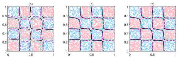
Figure 1: Nonlinear classification experiments. $(a)$ Newton method based equation (9). $(b)$ Newton method based equation (10). $(c)$ Newton method based equation (15). The training samples of class $1$ are plotted as lightskyblue plus ($\color[rgb]{0.53125,0.80859375,0.98046875}{+}$), and the training samples of class $0$ are plotted as lightpink circle ($\color[rgb]{1,0.71484375,0.7578125}{\circ}$). The solid black lines are the classification boundaries; the cyan dashed line and the magenta dashed line are the lines with predicted probabilities of 0.25 and 0.75, respectively. The test accuracies for the corresponding methods are 0.9585, 0.9584 and 0.9584 on 625 test samples, and the training time for the corresponding methods are 109.63s, 7.49s and 0.05s on 3375 train samples.

In Fig. 1, it can be seen that the classification boundaries of the three Newton methods are almost the same. From the contour line of the predicted probability, the first method has more samples with the predicted probability between 0.25 and 0.75 than the latter two methods. The test accuracies for the corresponding methods are 0.9585, 0.9584 and 0.9584 on 625 test samples, and the training time for the corresponding methods are 109.63s, 7.49s and 0.05s on 3375 train samples. This validates the efficiency of the fast Newton method based on the MCM approximation.

3.3 Fast Newton Method

We are now ready to develop a fast Newton method based on MCM approximation, which can reduce the time and space complexity more succinctly and effectively.

The main work of Newton method is the calculation of Newton direction. According to Theorem 1, $\boldsymbol{K}_{\boldsymbol{q}}+\tilde{\tau}\boldsymbol{I}$ is an MCM. By Theorem 2, we have

$${({\boldsymbol{K}_{\boldsymbol{q}}}+\tilde{\tau}\boldsymbol{I})^{-1}}=\frac{1}{n}{\boldsymbol{\phi}^{*}}(diag(\boldsymbol{v}+\tilde{\tau}\boldsymbol{1}))^{-1}\boldsymbol{\phi},$$

where $\boldsymbol{v}=\boldsymbol{\phi}\boldsymbol{k}$ is the vector of eigenvalues.

Then we rewrite (15) as follows:

$$\tilde{\boldsymbol{d}}\!=\!\frac{1}{n\tau}{\boldsymbol{\phi}^{*}}(diag(\boldsymbol{v}+\tilde{\tau}\boldsymbol{1}))^{-1}\boldsymbol{\phi}(\boldsymbol{y}\!-\!\tilde{\boldsymbol{p}}\!-\!n\lambda\boldsymbol{\alpha}).$$ (16)

In addition, replacing $\boldsymbol{K}$ with $\boldsymbol{K}_{\boldsymbol{q}}$ generated by Algorithm 1, we note the approximations of the objective function (3) and its gradient (5) as follows.

$$\tilde{F}(\boldsymbol{\alpha})\! =\frac{\lambda}{2}\!{\boldsymbol{\alpha}^{\top}\!}{\boldsymbol{K}\!_{\boldsymbol{q}}\!}\boldsymbol{\alpha}\!-\!\frac{1}{n}\!({\boldsymbol{y}^{\top}\!}\ln\tilde{\boldsymbol{p}}\!+{(\boldsymbol{1}-\boldsymbol{y})\!^{\top}\!}\ln(\boldsymbol{1}\!-\tilde{\boldsymbol{p}}\!)),$$ (17)

$$\nabla\tilde{F}(\boldsymbol{\alpha}) ={\boldsymbol{K}_{\boldsymbol{q}}}(\lambda\boldsymbol{\alpha}-\frac{1}{n}(\boldsymbol{y}-\tilde{\boldsymbol{p}})).$$ (18)

Now we present the detailed flow of the Fast Newton method based on MCM approximation in Algorithm 3.3.

Algorithm 2 Fast Newton method based on MCM

1:Training set $\mathbb{D}$, parameters $\sigma$, $\lambda$, ${T}$, $\varepsilon$, $\delta\in(0,1)$, $\beta\in(0,0.5)$ and given an initial $\boldsymbol{\alpha}_{0}$.

2:$\boldsymbol{\alpha}$.

3:Calculate $[\boldsymbol{k}_{\boldsymbol{i}}:\boldsymbol{i}\in[\boldsymbol{q}]]$ according to Algorithm 1.

4:Calculate $\boldsymbol{v}=\boldsymbol{\phi}[\boldsymbol{k}_{\boldsymbol{i}}:\boldsymbol{i}\in[\boldsymbol{q}]]$ by mFFT.

5:Calculate $\tilde{\boldsymbol{p}}$, $\nabla\tilde{F}({\boldsymbol{\alpha}_{0}})$ and $\tilde{F}({\boldsymbol{\alpha}_{0}})$.

6:while $t\leqslant T_{max}$ and $\text{ ∇}\tilde{\text{F}}\text{(}\text{α}\text{\_t) }\text{ > }\text{ε }\text{do}\text{<div id="alg2.l7nest" class="ltx\_listingline ltx\_markedasmath"> <span class="ltx\_tag ltx\_tag\_listingline"><span id="alg2.l7.1.1.1nest" class="ltx\_text" style="font-size:80\%;">7:</span></span><span id="alg2.l7.2nest" class="ltx\_text ltx\_font\_italic"> </span>Calculate </div>}\text{η}\text{= (1/}\text{τ}\text{)(}\text{y}\text{ - }\tilde{\text{p}}\text{- n}\text{λ}\text{α}\text{\_t)}.\text{8:88 Calculate}\text{δ}\text{= }\text{ϕη}\mathrm{b}\mathrm{y}\mathrm{m}\mathrm{F}\mathrm{F}\mathrm{T}.\text{9:99 Calculate}\text{ζ}\text{= (diag(}\text{v}\text{ + }\widetilde{\text{τ}}\text{1}\text{))^-1}\text{δ}.\text{10:1010 Calculate}\tilde{\text{d}}\text{= }\frac{\text{1}}{\text{n}}\text{ϕ}\text{^*}\text{ζ}\mathrm{u}\mathrm{s}\mathrm{i}\mathrm{n}\mathrm{g}\mathrm{i}\mathrm{n}\mathrm{v}\mathrm{e}\mathrm{r}\mathrm{s}\mathrm{e}\mathrm{m}\mathrm{F}\mathrm{F}\mathrm{T}.\text{11:1111 (Armijolines}$