Classifier construction in Boolean networks using algebraic methods

Abstract

We investigate how classifiers for Boolean networks (BNs) can be constructed and modified under constraints. A typical constraint is to observe only states in attractors or even more specifically steady states of BNs. Steady states of BNs are one of the most interesting features for application. Large models can possess many steady states. In the typical scenario motivating this paper we start from a Boolean model with a given classification of the state space into phenotypes defined by high-level readout components. In order to link molecular biomarkers with experimental design, we search for alternative components suitable for the given classification task. This is useful for modelers of regulatory networks for suggesting experiments and measurements based on their models. It can also help to explain causal relations between components and phenotypes. To tackle this problem we need to use the structure of the BN and the constraints. This calls for an algebraic approach. Indeed we demonstrate that this problem can be reformulated into the language of algebraic geometry. While already interesting in itself, this allows us to use Gröbner bases to construct an algorithm for finding such classifiers. We demonstrate the usefulness of this algorithm as a proof of concept on a model with 25 components.

Keywords: Boolean networks, Algebraic geometry, Gröbner bases, Classifiers.

1 Motivation

For the analysis of large regulatory networks so called Boolean networks (BNs) are used among other modeling frameworks [32, 1, 26]. They have been applied frequently in the past [22, 34, 18, 3]. In this approach interactions between different components of the regulatory networks are modeled by logical expressions. Formally, a Boolean network is simply a Boolean function $f:\{0,1\}^{n}\rightarrow\{0,1\}^{n}$, $n\in\mathbb{N}$. This Boolean function contains the information about the interactions of the components in the network. It is then translated into a so called state transition graph (STG). There are several slightly different formalisms for the construction of the STG of a BN. In all cases, the resulting state transition graph is a directed graph over the set of vertices $\{0,1\}^{n}$. The vertices of the STG are also called states in the literature about Boolean networks.

Modelers of regulatory networks are frequently – if not to say almost always – confronted with uncertainties about the exact nature of the interactions among the components of the network. Consequently, in many modeling approaches models may exhibit alternative behaviors. In so called asynchronous Boolean networks for example each state in the state transition graph can have many potential successor states (see e.g. [9]). More fundamentally, alternative models are constructed and then compared with each other (see e.g. [33, 37]).

To validate or to refine such models we need to measure the real world system and compare the results with the model(s). However, in reality for networks with many components it is not realistic to be able to measure all the components. In this scenario there is an additional step in the above procedure in which the modeler first needs to select a set of components to be measured which are relevant for the posed question. This scenario motivates our problem here. How can a modeler decide which components should be measured? It is clear that the answer depends on the question posed to the model and on the prior knowledge or assumptions assumed to be true.

When formalizing this question we are confronted with the task to find different representations of partially defined Boolean functions. In the field of logical analysis of data (LAD) a very similar problem is tackled [4, 2, 23, 11]. Here a list of binary vectorized samples needs to be extended to a Boolean function – a so called theory (see e.g. [11, p. 160]). In the literature of LAD this problem is also referred to as the Extension-Problem [11, p. 161 and p. 170]. Here reformulations into linear integer programs are used frequently [11]. However, they are more tailored to the case where the partially defined Boolean functions are defined explicitly by truth tables. In contrast to the scenario in LAD in our case the sets are typically assumed to be given implicitly (e.g. by so called readout components).

A common assumption in the field of Boolean modeling is that attractors play an important role. Attractors of BNs are thought to capture the long term behavior of the modeled regulatory network. Of special interest among these attractors are steady states (defined by $f(x)=x$ for a BN $f$). Consequently, a typical scenario is that the modeler assumes to observe only states of the modeled network which correspond to states belonging to attractors or even only steady states of the STG. The state space is then often partitioned by so-called readout components into phenotypes.

Our first contribution will be a reformulation of the above problem into the language of algebraic geometry. For this purpose we focus on the case of classification into two phenotypes. This is an important special case. Solutions to the more general case can be obtained by performing the algorithm iteratively. The two sets of states $A_{1}$ and $A_{2}$ in $\{0,1\}^{n}$ describing the phenotypes will be defined by some polynomial equations in the components of the network. This algebraic reformulation is possible since we can express the Boolean function $f:\{0,1\}^{n}\rightarrow\{0,1\}^{n}$ with polynomials over $\mathbb{F}_{2}[x_{1},\dots,x_{n}]$ – the polynomial ring over the finite field of cardinality two (see 2). In this way we relate the problem to a large well-developed theoretical framework. Algebraic approaches for the construction and analysis of BNs and chemical reaction systems have been used in the past already successfully (see e.g. [24, 40, 27]). Among other applications they have been applied to the control of BNs [30] and to the inference of BNs from data [38, 41].

Our second contribution will be to use this algebraic machinery to construct a new algorithm to find alternative classifiers. To our knowledge this is the first algorithm that is able to make use of the implicit description of the sets that should be classified. For this algorithm we use Gröbner bases. Gröbner bases are one of the most important tools in computational algebraic geometry and they have been applied in innumerous applications, e.g. cryptography [17], statistics [15], robotics [7], biological dynamical systems [14, 25, 30, 39]. Specialized algorithms for the computations of Gröbner bases have been developed for the Boolean case and can be freely accessed [5]. They are able to deal with with systems of Boolean polynomials with up to several hundreds variables [5] using a specialized data structure (so called zero-suppressed binary decision diagram (ZDD) [29]). Such approaches are in many instances competitive with conventional solvers for the Boolean satisfiability problem (SAT-solvers) [5].

Our paper is structured in the following way. We start by giving the mathematical background used in the subsequent sections in 2. In 3 we formalize our problem. We then continue in 4 to give a high-level description of the algorithm we developed for this problem. More details about the used data structures and performance can be found in 5. As a proof of concept we investigate in 6 a BN of $25$ components modeling cell-fate decision [8]. We conclude the paper with discussing potential ways to improve the algorithm.

2 Mathematical background

In the course of this paper we need some concepts and notation used in computational algebraic geometry. For our purposes, we will give all definitions for the field of cardinaliy two denoted by $\mathbb{F}_{2}$ even though they apply to a much more general setting. For a more extensive and general introduction to algebraic geometry and Gröbner bases we refer to [12].

We denote the ring of polynomials in $x_{1},\dots,x_{n}$ over $\mathbb{F}_{2}$ with $\mathbb{F}_{2}[x_{1},\dots,x_{n}]$. For $n\in\mathbb{N}$, let $[n]:=\{1,\dots,n\}$. Given $\alpha=(\alpha_{1},\dots,\alpha_{n})\in\mathbb{Z}_{\geq 0}^{n}$, we denote by $x^{\alpha}$ the monomial $\prod_{i}x_{i}^{\alpha_{i}}$ in $\mathbb{F}_{2}[x_{1},\dots,x_{n}]$. For $f_{1},\dots,f_{k}$ in $\mathbb{F}_{2}[x_{1},\dots,x_{n}]$ we denote with $\langle f_{1},\dots,f_{k}\rangle$ a so-called ideal in $\mathbb{F}_{2}[x_{1},\dots,x_{n}]$ – a subset of polynomials which is closed under addition and multiplication with elements in $\mathbb{F}_{2}[x_{1},\dots,x_{n}]$ – generated by these polynomials. The set of Boolean functions – that is the set of functions from $\mathbb{F}_{2}^{n}$ to $\mathbb{F}_{2}$ – will be denoted by $\mathbb{B}(n)$. When speaking about Boolean functions and polynomials in $\mathbb{F}_{2}[x_{1},\dots,x_{n}]$ we need to take into account that the set of polynomials $\mathbb{F}_{2}[x_{1},\dots,x_{n}]$ does not coincide with the set of Boolean functions. This is the case since the so-called field polynomials $x_{1}^{2}-x_{1}$, $\dots$, $x_{n}^{2}-x_{n}$ evaluate to zero over $\mathbb{F}_{2}^{n}$ [20]. Consequently, there is not a one-to-one correspondence between polynomials and Boolean functions. However, we can say that any two polynomials whose difference is a sum of field polynomials corresponds to the same Boolean function (see e.g. [10]). In other words we can identify the ring of Boolean functions $\mathbb{B}(n)$ with the quotient ring $\mathbb{F}_{2}[x_{1},\dots,x_{n}]/\langle x_{1}^{2}-x_{1},\dots,x_{n}^{2}-x_{n}\rangle$. We will denote both objects with $\mathbb{B}(n)$. A canonical system of representatives of $\mathbb{B}(n)$ is linearly spanned by the the square-free monomials in $\mathbb{F}_{2}[x_{1},\dots,x_{n}]$. Hence, in what follows when we talk about a Boolean function $f\in\mathbb{B}(n)$ as a polynomial in the variables $x_{1},\dots,x_{n}$ we refer to the unique polynomial in $\mathbb{F}_{2}[x_{1},\dots,x_{n}]$ which involves only monomials that are square-free and agrees with $f$ as a Boolean function.

Since we are interested in our application in subsets of $\mathbb{F}_{2}^{n}$, we need to explain their relationship to the polynomial ring $\mathbb{F}_{2}[x_{1},\dots,x_{n}]$. This relationship is established using the notion of the vanishing ideal. Instead of considering a set $B\subseteq\mathbb{F}_{2}^{n}$ we will look at its vanishing ideal $\mathcal{I}(B)$ in $\mathbb{B}(n)$. The vanishing ideal of $B$ consists of all Boolean functions which evaluate to zero on $B$. Conversely, for an ideal $\mathcal{I}$ in $\mathbb{B}(n)$ we denote with $\mathcal{\mathcal{V}}(\mathcal{I})$ the set of points in $\mathbb{F}_{2}^{n}$ for which every Boolean function in $\mathcal{I}$ evaluates to zero. Due to the Boolean Nullstellensatz (see [35, 19]) there is an easy relation between a set $B\subseteq\mathbb{F}_{2}^{n}$ and its vanishing ideal $\mathcal{I}(B)$: For an ideal $\mathcal{I}$ in $\mathbb{B}(n)$ such that $\mathcal{\mathcal{V}}(\mathcal{I})\not=\emptyset$ and for any polynomial $h\in\mathbb{B}(n)$ it holds

$$h\in\mathcal{I}\Leftrightarrow\forall v\in\mathcal{\mathcal{V}}(\mathcal{I}):h(v)=0.$$

In this paper, we will consider Boolean functions whose domain is restricticted to certain states (e.g. attractors or steady states). Hence, there are different Boolean functions that behave in the same way when we restrict their domain.

Example 1.

Consider the set $B:=\{000,110,101,011\}$. Consider the Boolean function $f:=x_{1}$ and $g:=x_{2}+x_{3}$. Both Boolean functions are different, i.e., $f(1,1,1)=1$ and $g(1,1,1)=0$, but they agree over $B$.

$$\begin{array}[]{c | c | c | c | c}&000&110&101&011\\ \hline\cr f&0&1&1&0\\ g&0&1&1&0\end{array}.$$

Note that $\mathcal{I}(B)=\langle x_{1}+x_{2}+x_{3}\rangle$, that is, the ideal $\mathcal{I}(B)$ is generated by the Boolean function $x_{1}+x_{2}+x_{3}$ since it is the unique Boolean function vanishing only on $B$. ∎

Given a set $B$, we write $\mathbb{B}(n)/\mathcal{I}(B)$ to refer to the set of all the different Boolean functions on $B$. As we saw in the previous example, different Boolean functions agree on $B$. Hence, we will be interested in how to obtain certain representatives of the Boolean function in $\mathbb{B}(n)/\mathcal{I}(B)$ algorithmically. In our application, the set $\mathbb{B}(n)/\mathcal{I}(B)$ will become the set of all possible classifiers we can construct that differ on $B$. To obtain specific representatives of a Boolean function in $\mathbb{B}(n)/\mathcal{I}(B)$ we will use Gröbner bases. A Gröbner basis of an ideal is a set of generators of the ideal with some extra properties related to monomial orderings. A monomial ordering is a total ordering on the set of monomials in $\mathbb{F}_{2}[x_{1},\dots,x_{n}]$ satisfying some additional properties to ensure the compatibility with the algebraic operations in $\mathbb{F}_{2}[x_{1},\dots,x_{n}]$ (see [12, p. 69] for details).

For any polynomial in $p\in\mathbb{F}_{2}[x_{1},\dots,x_{n}]$ and monomial ordering $\prec$, we denote the initial monomial of $p$ by $in_{\prec}(p)$, that is the largest monomial appearing in $p$ with respect to $\prec$. We are interested in specific orderings – the lexicographical orderings – on these monomials. As we will see, the usage of lexicographical orderings in the context of our application will allow us to look for classifiers which are optimal in a certain sense.

Definition 2.1 ([12, p. 70]).

Let $\alpha=\begin{pmatrix}\alpha_{1}&\dots&\alpha_{n}\end{pmatrix}$ and $\beta=\begin{pmatrix}\beta_{1}&\dots&\beta_{n}\end{pmatrix}$ be two elements in $\mathbb{Z}_{\geq 0}^{n}$. Given a permutation $\sigma$ of $\{1,\dots,n\}$, we say $x^{\alpha}\succ_{lex(\sigma)}x^{\beta}$ if there is $k\in[n]$ such that

$$(\forall i<k:\,\alpha_{\sigma(i)}=\beta_{\sigma(i)})\text{ and }\alpha_{\sigma(k)}>\beta_{\sigma(k)}.$$

Definition 2.2 ([36, p. 1]).

Let $\prec$ be any monomial ordering. For an ideal $\mathcal{I}\subseteq\mathbb{F}_{2}[x_{1},\dots,x_{n}]$ we define its initial ideal as the ideal

$$in_{\prec}(\mathcal{I}):=\langle in_{\prec}(f)|f\in\mathcal{I}\rangle.$$

A finite subset $G\subseteq\mathcal{I}$ is a Gröbner basis for $\mathcal{I}$ with respect to $\prec$ if $in_{\prec}(\mathcal{I})$ is generated by $\{in_{\prec}(g)|g\in G\}$. If no element of the Gröbner basis $G$ is redundant, then $G$ is minimal. It is called reduced if for any two distinct elements $g,g^{\prime}\in G$ no monomial in $g^{\prime}$ is divisible by $in_{\prec}(g)$. Given an ideal and a monomial ordering, there is a unique minimal reduced Gröbner basis involving only monic polynomials; we denote it by $G_{\prec}(\mathcal{I})$. Every monomial not lying in $in_{\prec}(\mathcal{I})$ is called standard monomial.

We can extend the monomial orderings to partial orderings of polynomials on $\mathbb{F}_{2}[x_{1},\dots,x_{n}]$. Consider polynomials $f,g\in\mathbb{F}_{2}[x_{1},\dots,x_{n}]$ and a monomial ordering $\succ$. We say that $f\succ g$ if $in_{\prec}(f)\succ in_{\prec}(g)$ or $f-in_{\prec}(f)\succ g-in_{\prec}(g)$. The division algorithm rewrites every polynomial $f\in\mathbb{F}_{2}[x_{1},\dots,x_{n}]$ modulo $\mathcal{I}$ uniquely as a linear combination of these standard monomials [12, Ch. 2]. The result of this algorithm is called Normal form. For the convenience of the reader, we state this in the following lemma and definition.

Lemma 2.1 (Normal form).

Given a monomial ordering $\succ$, $f\in\mathbb{B}(n)$ and an ideal $\mathcal{I}$ there is a unique $g\in\mathbb{B}(n)$ such that $f$ and $g$ represent the same Boolean function in $\mathbb{B}(n)/\mathcal{I}$ and $g$ is minimal with respect to the ordering $\succ$ among all the Boolean functions equivalent to $f$ in $\mathbb{B}(n)/\mathcal{I}$. We call $g$ the normal form of $f$ modulo $I$ denoted by $\mathrm{NF}_{\mathcal{I}}(\succ,f)$.

Example 2 (Cont.).

Consider the permutation $\sigma$ of $\{1,2,3\}$ such that $\sigma(i):=4-i$. Then, $\mathrm{NF}_{\mathcal{I}}(\succ_{\sigma},f)=\mathrm{NF}_{\mathcal{I}}(\succ_{\sigma},g)=x_{1}$. Hence, if we choose a “good” monomial ordering, we can get simpler Boolean functions involving less variables. ∎

3 Algebraic formalization

As discussed in 1, we start with the assumption that we are given a set of Boolean vectors $B$ in $\mathbb{F}_{2}^{n}$ representing the observable states. In our applications these states are typically attractors or steady states of a BN. We also assume that our set $B$ is partitioned into a set of phenotypes, i.e. $B=A_{1}\cup\cdots\cup A_{k}$. Our goal is then to find the components that allow us to decide for a vector in $B$ to which set $A_{i}$, $i\in[k]$, it belongs. For a set of indices $I\subseteq[n]$ and $x\in\mathbb{F}_{2}^{n}$, let us denote with $\text{proj}^{I}(x)$ the projection of $x$ onto the components $I$. Our problem could be formalized in the following way.

Problem 3.1 (State-Discrimination-Problem).

For a given partition of non-empty sets $A_{1},\dots,A_{k}$ ($k\geq 2$) of states $B\subseteq\{0,1\}^{n}$, find the sets of components $\emptyset\not=I\subseteq[n]$ such that $\text{proj}^{I}(A_{1}),\dots,\text{proj}^{I}(A_{k})$ forms a partition of $\text{proj}^{I}(B)$.

Clearly, since the sets $A_{1},\dots,A_{k}$ form a partition of $B$, we can decide for each state $x$ in $B$ to which set $A_{i}$ it belongs. If $I\subseteq[n]$ is a solution to 3.1, this decision can be only based on $\text{proj}^{I}(x)$ as $\text{proj}^{I}(A_{1}),\dots,\text{proj}^{I}(A_{k})$ form a partition of $\text{proj}^{I}(B)$. As we discussed in 1, 3.1 is equivalent to Extension-Problem [11, p. 161 and p. 170]. However, in our case the sets in 3.1 are typically given implicitly. That is, we are given already some information about the structure of the sets in the above problem. This calls for an algebraic approach. We consider the case in 3.1 where $k$ equals two. This is an important special case since many classification problems consist of two sets (e.g. healthy and sick). Furthermore, solutions to the more general case can be obtained by considering iteratively the binary case (see also the case study in 6).

Let $\mathcal{I}(B)\subseteq\mathbb{F}_{2}[x_{1},\dots,x_{n}]$ be the vanishing ideal of a set $B\subseteq\mathbb{F}_{2}^{n}$. Let $f:\mathbb{F}_{2}^{n}\rightarrow\mathbb{F}_{2}$ be a Boolean function which can be identified with an element in $\mathbb{B}(n):=\mathbb{F}_{2}[x_{1},\dots,x_{n}]\big{/}\langle x_{1}^{2}-x_{1},\dots,x_{n}^{2}-x_{n}\rangle$. We want to find representatives of $f$ in $\mathbb{B}(n)\big{/}\mathcal{I}(B)$ which depend on a minimal set of variables with respect to set inclusion or cardinality. We express this in the following form:

Problem 3.2.

For $f\in\mathbb{B}(n)$ and $B\subseteq\mathbb{F}_{2}^{n}$, find the representatives of $f$ in $\mathbb{B}(n)\big{/}\mathcal{I}(B)$ which depend on a set of variables satisfying some minimality criterion.

It is clear that 3.2 is equivalent to 3.1 for the case $k=2$ since due to the Boolean Strong Nullstellensatz (see [35]) a Boolean function $f$ is zero on $B$ if and only if $f$ is in $\mathcal{I}(B)$. Therefore, all Boolean functions which are in the same residue class as $f$ agree with it as Boolean functions on $B$ and vice versa. The sets of variables each representative depends on are the solutions to 3.2. The representatives are then the classifiers.

Here we will focus on solutions of 3.2 which are minimal with respect to set inclusion or cardinality. However, also other optimality criteria are imaginable. For example one could introduce some weights for the components. Let us illustrate 3.2 with a small example.

Example 3.

Consider the set $B=\{000,111,011,101\}\subset\mathbb{F}_{2}^{3}$. Then $\mathcal{I}(B)\subseteq\mathbb{B}(3)$ is given by $\langle\overbrace{x_{1}x_{2}+x_{1}+x_{2}+x_{3}}^{=:f}\rangle$ since $f$ is the unique Boolean function that is zero on $B$ and one on it complement. Let $\varphi(x)=x_{1}x_{2}x_{3}$. It is easy to check that for example $x_{1}x_{3}+x_{2}x_{3}+x_{3}$ and $x_{1}x_{2}$ are different representatives of $\varphi$ in $\mathbb{B}(3)\big{/}\mathcal{I}(B)$. The representative $x_{1}x_{2}$ depends only on two variables while the other two representatives depend on three. ∎

We can obtain a minimal representative of $f$ in 3.2 by computing $\mathrm{NF}_{\mathcal{I}}(\prec,f)$ for a suitable lexicographical ordering $\prec$.

Proposition 3.1.

Given a set of points $B\subset\mathbb{F}_{2}^{n}$ and a Boolean function $f\in\mathbb{B}(n)$ assume, with no loss of generality, that there is an equivalent Boolean function $g\in\mathbb{F}_{2}[x_{1},\dots,x_{n}]$ modulo $\mathcal{I}(B)$ involving only $x_{k},\dots,x_{n}$. Consider a permutation $\sigma$ of $\{1,\dots,n\}$ such that $\sigma(\{k,\dots,n\})=\{k,\dots,n\}$. Then, the only variables appearing in $\mathrm{NF}_{I}(\prec_{lex(\sigma)},f)=\mathrm{NF}_{I}(\prec_{lex(\sigma)},g)$ are the ones in $\{x_{k},\dots,x_{n}\}$. In particular, if there is no Boolean function equivalent to $f$ modulo $\mathcal{I}(B)$ involving a proper subset of $\{x_{k},\dots,x_{n}\}$, then $\mathrm{NF}_{I}(\prec_{lex(\sigma)},f)=\mathrm{NF}_{I}(\prec_{lex(\sigma)},g)$ involves all the variables in $\{x_{k},\dots,x_{n}\}$.

Proof.

The proof follows from the minimality of $\mathrm{NF}_{I}(\prec_{lex(\sigma)},f)$ with respect to $\prec_{lex(\sigma)}$. Note that, because of the lexicographical ordering $\prec_{lex(\sigma)}$, any Boolean function equivalent to $f$ modulo $\mathcal{I}(B)$ involving variables in $\{x_{1},\dots,x_{k-1}\}$ will be bigger than $g$, so it cannot be minimal. ∎

4 Description of the Algorithm

Clearly we could use 3.1 to obtain an algorithm that finds the minimal representatives of $\varphi$ in $\mathbb{B}(n)/\mathcal{I}(B)$ by iterating over all lexicographical orderings in $\mathbb{F}_{2}[x_{1},\dots,x_{n}]$. However, this naive approach has several drawbacks:

1. The number of orderings over $\mathbb{B}(n)$ is growing rapidly with $n$ since there are $n!$ many lexicographical orderings over $\mathbb{B}(n)$ to check.

2. We do not obtain for every lexicographical ordering a minimal representative. Excluding some of these orderings “simultaneously” could be very beneficial.

3. Different monomial orderings can induce the same Gröbner bases. Consequently, the normal form leads to the same representative.

4. Normal forms with different monomial orderings can result in the same representative. If we detect such cases we avoid unnecessary computations.

We describe now an algorithm addressing the first two points. Recall that for a monomial ordering $\succ$ and $f\in\mathbb{B}(n)$, we use the notation $\mathrm{NF}_{\mathcal{I}}(\succ,f)$ to denote the normal form of $f$ in $\mathbb{B}(n)/\mathcal{I}$ with respect to $\succ$. When $\mathcal{I}$ is clear from the context, we write $\mathrm{NF}(\succ,f)$. We denote with $\varphi$ any representative of the indicator function of $A$ in $\mathbb{B}(n)\big{/}\mathcal{I}(B)$. Let $\mathrm{Var}(\varphi)$ be the variables occurring in $\varphi$ and $\mathrm{Comp}(\varphi)$ be its complement in $\{x_{1},\dots,x_{n}\}$. Instead of iterating through the orderings on $\mathbb{B}(n)$, we consider candidate sets in the power set of $\{x_{1},\dots,x_{n}\}$, denoted by $\mathscr{P}(x_{1},\dots,x_{n})$ (i.e. we initialize the family of candidate sets $P$ with $P\leftarrow\mathscr{P}(x_{1},\dots,x_{n})$). We want to find the sets $A$ in the family of candidate sets $P$ for which the equality $A=\mathrm{Var}(\varphi)$ holds for some minimal solution $\varphi$ to 3.2, that is, involving the minimal amount of variables. For each candidate set $A$ involving $k$ variables we pick a lexicographical ordering $\succ$ for which it holds $A^{c}\succ A$, i.e. for every variable $x_{i}\in A^{c}$ and $x_{j}\in A$ it holds $x_{i}\succ x_{j}$, where $A^{c}:=\{x_{1},\dots,x_{n}\}\setminus A$. This approach is sufficient to find the minimal solutions as we will argue below. This addresses the first point above since there are $2^{n}$ candidate sets to consider while there are $n!$ many orderings.

4.1 Excluding candidate sets

To address the second point we will exclude after each reduction step a family of candidate sets. If, for an ordering $\succ$, we computed a representative $\mathrm{NF}(\succ,\varphi)$ we can, independently of the minimality of $\mathrm{NF}(\succ,\varphi)$, exclude some sets in $P$. To do so, we define for any set $A\subseteq\{x_{1},\dots,x_{n}\}$ the following families of sets:

$$\mathcal{\text{FORWARD}}(A) :=\big{\{}B\subseteq\{x_{1},\dots,x_{n}\}|A\subset B\big{\}},$$

$$\text{$\mathcal{\text{FORWARDEQ}}$}(A) :=\big{\{}B\subseteq\{x_{1},\dots,x_{n}\}|A\subseteq B\big{\}},$$

$$\text{$\mathcal{\text{BACKWARD}}$}(A) :=\big{\{}B\subseteq\{x_{1},\dots,x_{n}\}|B\subseteq A\big{\}},$$

$$\mathcal{\text{SMALLER}}(A,\succ) :=\big{\{}x\in\{x_{1},\dots,x_{n}\}|\exists y\in A:y\succ x\big{\}},$$

$$\mathcal{\text{SMALLEREQ}}(A,\succ) :=\big{\{}x\in\{x_{1},\dots,x_{n}\}|\exists y\in A:y\succeq x\big{\}}.$$

It is clear that, if we obtain in a reduction step a representative $\phi=\mathrm{NF}(\succ,\varphi)$, we can exclude the sets in $\mathcal{\text{FORWARD}}(\mathrm{Var}(\phi))$ from the candidate sets $P$. But, as we see in the following lemma, we can exclude even more candidate sets.

Lemma 4.1.

Let $\succ$ be a lexicographical ordering and let $\phi=\mathrm{NF}(\succ,\varphi)$ be the corresponding normal form of $\varphi$. Then none of the sets $A\subseteq\mathcal{\text{SMALLER}}(\mathrm{Var}(\phi),\succ)$ can belong to a minimal solution to 3.2.

Proof.

Assume the contrary, that is there is a minimal solution $\psi$ with $\mathrm{Var}(\psi)\subseteq\mathcal{\text{SMALLER}}(\mathrm{Var}(\phi),\succ)$. It follows that, by the definition of lexicographical orderings, there is at least one $y\in\mathrm{Var}(\phi)$ with $y\succ\mathrm{Var}(\psi)$. Consequently, $\psi$ is smaller than $\phi$ with respect to $\succ$ which cannot happen by the definition of the normal form. ∎

If we also take the structure of the polynomials into account, we can improve 4.1 further. For this purpose, we look at the initial monomial of $\phi=\mathrm{NF}(\succ,\varphi)$ with respect to $\succ$, $M:=in_{\succ}(\phi)$. We consider the sets $\mathrm{Var}(M)$ and $\mathrm{Comp}(M)$. Given a variable $x_{i}\in\{x_{1},\dots,x_{n}\}$ and a subset $S\subseteq\{x_{1},\dots,x_{i}\}$, let $S_{\succ x_{i}}$ be the set of variables in $S$ bigger than $x_{i}$, i.e.

$$S_{\succ x_{i}}:=\big{\{}x_{j}\in S|x_{j}\succ x_{i}\big{\}}.$$

Lemma 4.2.

Consider a lexicographical ordering $\succ$. Let $\phi=\mathrm{NF}(\succ,\varphi)$ and $M=in_{\succ}(\text{$\phi$})$. If $x_{i}\in\mathrm{Var}(M)$, then any set $S\subseteq\mathcal{\text{SMALLEREQ}}(\mathrm{Var}(\phi),\succ)$ with $x_{i}\not\in S$ and $S\cap Comp_{\succ x_{i}}(M)=\emptyset$ cannot belong to a minimal solution to 3.2.

Proof.

Note that $\prod_{j\in S}x_{j}\prec M$ as $M$ involves $x_{i}$ but $\prod_{j\in S}x_{j}$ only involves variables smaller than $x_{i}$. Then, the proof is analogous to 4.1 using the fact that any minimal solution involving only variables in $S$ has monomials smaller or equal than $\prod_{j\in S}x_{j}\prec M$. Hence, $\phi$ is not minimal with respect to $\prec$. ∎

In particular, 4.2 entails the case where the initial monomial of $\mathrm{NF}(\succ,\varphi)$ is a product of all variables occurring in $\mathrm{NF}(\succ,\varphi)$. In this case, for every subset $S\subseteq\mathrm{Var}(\phi)\subseteq\mathcal{\text{SMALLEREQ}}(\mathrm{Var}(\phi),\succ)$ it holds $S\cap\mathrm{Comp}(M)=S\cap\mathrm{Comp}(\phi)=\emptyset$. Therefore, according to 4.2 $\mathrm{NF}(\succ,\varphi)$ is minimal.

For a lexicographical ordering $\succ$ and a normal form $\phi=\mathrm{NF}(\succ,\varphi)$ we can, using 4.2, exclude the families of sets in (4.1) from the set of candidates $P$.

$$\mathcal{\text{BACKWARD}}(S_{i})\text{ with }x_{i}\in\mathrm{Var}(in_{\succ}(\phi))\text{ and}$$ (4.1)

$$S_{i}:=\mathcal{\text{SMALLEREQ}}(\mathrm{Var}(\phi),\succ)\backslash\big{(}\{x_{i}\}\cup Comp_{\succ x_{i}}(in_{\succ}(\phi))\big{)}$$

We illustrate this fact with a small example:

Example 4.

Consider a lexicographical ordering $\succ$ with $x_{4}\succ\cdots\succ x_{1}$ and a normal form $\phi=\mathrm{NF}(\succ,\varphi)$ with initial monomial $x_{4}x_{2}$. Then, we can exclude from $P$ the sets in $\mathcal{\text{BACKWARD}}(\{x_{3},x_{2},x_{1}\})$ and $\mathcal{\text{BACKWARD}}(\{x_{4},x_{1}\})$. ∎

Note that if we consider, instead of lexicographical orderings, graded monomial orderings, then we obtain the following version of 4.2. This is useful to lower bound the number of variables in a minimal solution. Also, it could be useful when considering different optimality criteria.

Lemma 4.3.

Let $\succ$ be a graded monomial ordering [12, Ch. 8.4]. Then, the total degree $d$ of $\mathrm{NF}(\succ,\varphi)$ is smaller or equal to the number of variables involved in any minimal representation of $\varphi$.

Proof.

Assume that $\varphi$ has a representation involving less than $d$ variables. Then, this representation has to have degree less than $d$ (because every monomial is square-free). Hence, we get a contradiction because $\mathrm{NF}(\succ,\varphi)$ is not minimal. ∎

We can now use the results above to construct 1. In each step of our algorithm we choose a candidate set $A$ of $P$ and an ordering $\succ$ satisfying $A^{c}\succ A$. Then we compute the reduction of $\varphi$ with respect to $\succ$ with the corresponding Gröbner basis. Let us call the result $\phi$. After each reduction in 1 we exclude from $P$ the sets that we already checked and the sets we can exclude with the results above. That is, we can exclude from $P$ the candidate sets $\mathcal{\text{FORWARDEQ}}(\mathrm{Var}(\phi))$ (Line $9$ in 1) and according to 4.2 the family of sets $\mathcal{\text{BACKWARD}}(S_{i})\text{ with }x_{i}\in\mathrm{Var}(in_{\prec}(\phi))$ where $S_{i}$ is defined according to (4.1). The algorithm keeps doing this until the set of candidate sets is empty. To be able to return the solutions we keep simultaneously track of the set of potential solutions denoted by $S$. Initially this set equals $P$. But since we subtract from $S$ not the set $\mathcal{\text{FORWARDEQ}}(\mathrm{Var}(\phi))$ but $\mathcal{\text{FORWARD}}(\mathrm{Var}(\phi))$ we keep some of the sets that we checked already in $S$. This guarantees that $S$ will contain all solutions when $P$ is empty.

1:  $P\leftarrow\mathscr{P}(\{x_{1},\dots,x_{n}\})$

2:  $S\leftarrow\mathscr{P}(\{x_{1},\dots,x_{n}\})$

3:  while $P\not=\emptyset$ do

4:     $A\leftarrow\text{any set in }P$

5:     $\succ\leftarrow\text{any lexicographical ordering satisfying }\mathrm{Comp}(A)\succ A$

6:     $\varphi\leftarrow\mathrm{NF}(\succ,\varphi)$

7:     $V\leftarrow\mathrm{Var}(\varphi)$

8:     $P\leftarrow P-\mathcal{\text{FORWARDEQ}}(V)$

9:     $S\leftarrow S-\mathcal{\text{FORWARD}}(V)$

10:     for all $x_{i}$ in $\mathrm{Var}(in_{\prec}(\varphi))$ do

11:        $S_{i}\leftarrow\text{Compute $S_{i}$ according to Eq.(\ref{eq:Si})}$

12:        $P\leftarrow P-\mathcal{\text{BACKWARD}}(S_{i})$

13:        $S\leftarrow S-\mathcal{\text{BACKWARD}}(S_{i})$

14:     end for

15:  end while

16:  return  $S$

Algorithm 1 compute_solutions($\varphi$, $\{x_{1},\dots,x_{n}\}$, $\mathcal{I}$)

5 Implementation and benchmarking

When implementing 1 the main difficulties we face is an effective handling of the candidate sets. In each step in the loop in 1 we need to pick a new set $A$ from the family of candidate sets $P$. Selecting a candidate set from $P$ is not a trivial task since it structure can become very entangled. The subtraction of the sets $\mathcal{\text{FORWARD}}(\cdot)$ and $\mathcal{\text{BACKWARD}}(\cdot)$ from $P$ can make the structure of the candidate sets very complicated. In practice this a very time-consuming part of the algorithm. To tackle this problem we use a specialized data structure – so-called Zero-suppressed decision diagram (ZDDs) [28, 29] – to represent $P$. ZDDs are a type of Binary Decision Diagrams (BDDs). A binary decision diagram represents a Boolean function or a family of sets as a rooted directed acyclic graph. Specific reduction rules are used to obtain a compact, memory efficient representation. ZDDs can therefore effectively store families of sets. Furthermore, set operations can be computed directly on ZDDs. This makes them an ideal tool for many combinatorial problems [28]. We refer to the literature for a more detailed introduction to ZDDs [28, 29].

Our implementation in Python can be found at https://git.io/Jfmuc. For the Gröbner basis calculations as well as the ZDDs we used libraries from PolyBoRi (see [5]). The computation time for the network with 25 components considered in the case study in 6 was around 10 seconds on a personal computer with an intel core i5 vPro processor. Other networks we created for test purposes resulted in similar results (around 30 seconds for example1.py in the repository). However, computation time depends highly on the structure of the network and not only on its size. For a network even larger (example2.py in the repository with 38 components) computations took around two seconds while computations for a slightly different network of the same size (see example3.py in the repository) took around a minute. For a similar network (example4.py in the repository) we aborted the computation after one hour. In general, the complexity of computing Gröbner bases is highly influenced by algebraic properties such as the regularity of the vanishing ideal of the set we restrict our classifiers to. If the shapes of the sets in our algorithm are more regular (e.g. some components are fixed to zero or one) the number of candidate sets is reduced much faster by the algorithm. Similar, computations seem to be also often faster for networks with fewer regulatory links.

6 Case study

Let us consider the Boolean model constructed in [8] modeling cell-fate decision. These models can be used to identify how and under which conditions the cell chooses between different types of cell deaths and survival. The complete model can be found in the BioModels database with the reference MODEL0912180000. It consists of $25$ components. The corresponding Boolean function is depicted in 1. While in [8] the authors use a reduced model (see also [31]) to make their analysis more tractable, we can and do work with the complete model here.

The Boolean network depicted in 1 models the effect of cytokines such as TNF and FASL on cell death. In the Boolean model they correspond to input components. These cytokines can trigger cell death by apoptosis or necrosis (referred to as non-apoptotic cell death abbreviated by NonACD). Under different cellular conditions they lead to the activation of pro-survival signaling pathway(s). Consequently, the model distinguishes three phenotypes: Apoptosis, NonACD and Survival. Three corresponding signaling pathways are unified in their model. Finally, specific read-out components for the three phenotypes were defined. The activation of CASP3 is considered a marker for apoptosis. When MPT occurs and the level of ATP drops the cell enters non-apoptotic cell death. If Nf$\kappa$B is activated cells survive [8, p. 4]. This leads to the three classifiers in the model depicted in 2. Each classifier tells us to which cell fate (apoptosis, NonACD, survival) a state belongs.

We are interested in alternative classifiers on the set of attractors of the Boolean network. Let us denote the union of these attractors with $B$ (in agreement with the notation in 3.2). In this case all attractors are steady states (see [8, p. 4] for details). For illustrating our results we computed the steady states of the network using GINsim [21] (see 1). But this is not necessary for our calculations here. However, we can see that the classifiers given in [8] indeed result in disjoint sets of phenotypes.

Since the Boolean network in 1 possesses only steady states as attractors we can represent the ideal $\mathcal{I}(B)$ in 3.2 as $\langle f_{1}(x)+x_{1},\dots,f_{n}(x)+x_{n}\rangle$ where $f$ is the Boolean function depicted in 1.

Next, we computed for each of the classifiers alternative representations. In Table 3, we present the nine different minimal representations on $B$ of the classifier for NonACD. Among these options there are three ways how to construct a classifier based on one component (that is ATP, MPT or ROS). Also interestingly none of the components in the Boolean network is strictly necessary for the classification of the phenotypes. Consequently, there are potentially very different biological markers in the underlying modeled regulatory network. Despite this, there are some restrictions on the construction of the classifier, e.g., if we want to use the component Cytc, MOMP or SMAC we need to use also the component labeled as apoptosome. In total, the components useful for the classification of NonACD are ATP, CASP3, Cytc, MOMP, apoptosome, MPT, ROS and SMAC. The remaining $17$ components are redundant for this purpose.

We obtain similar results for the other two classifiers. For apoptosis we found $17$ alternative classifiers depicted in Table 4 involving the nine components (ATP, BAX, CASP8, Cytc, MOMP, SMAC, MPT, ROS, CASP3 and apoptosome). For the classifier for survival of the cell depicted in Table LABEL:tab:survival we found much more alternative classifiers ($84$ alternative classifiers). Most classifiers depend on four components. But we can observe that each of the components IKK, BCL2, NFKB1, RIP1ub, XIAP, cFLIP can be used for classification. Computations for each of the three classifiers took around $10$-$30$ seconds on a personal computer with an intel core i5 vPro processor in each case.

Component	Update function
$ATP$	$1+MPT$
$BAX$	$CASP8\cdot(1+BCL2)$
$BCL2$	$NFKB1$
$CASP3$	$(1+XIAP)\cdot apoptosome$
$CASP8$	$((1+DISCTNF)\cdot(1+DISCFAS)\cdot CASP3\cdot(1+cFLIP)+(1+DISCTNF)\cdot DISCFAS\cdot(1+cFLIP)+(1+DISCTNF)\cdot(1+DISCFAS)\cdot CASP3\cdot(1+cFLIP)+(1+DISCTNF)\cdot DISCFAS\cdot(1+cFLIP))\cdot DISCTNF\cdot(1+cFLIP)+((1+DISCTNF)\cdot(1+DISCFAS)\cdot CASP3\cdot(1+cFLIP)+(1+DISCTNF)\cdot DISCFAS\cdot(1+cFLIP)+(1+DISCTNF)\cdot(1+DISCFAS)\cdot CASP3\cdot(1+cFLIP)+(1+DISCTNF)\cdot DISCFAS\cdot(1+cFLIP))+DISCTNF\cdot(1+cFLIP)$
$Cytc$	$MOMP$
$DISCFAS$	$FASL\cdot FADD$
$DISCTNF$	$TNFR\cdot FADD$
$FADD$	$FADD$
$FASL$	$FASL$
$IKK$	$RIP1ub$
$MOMP$	$((1+BAX)\cdot MPT)\cdot BAX+((1+BAX)\cdot MPT)+BAX$
$MPT$	$(1+BCL2)\cdot ROS$
$NFKB1$	$IKK\cdot(1+CASP3)$
$NonACD$	$1+ATP$
$RIP1$	$(1+TNFR)\cdot DISCFAS\cdot(1+CASP8)\cdot TNFR\cdot(1+CASP8)+(1+TNFR)\cdot DISCFAS\cdot(1+CASP8)+TNFR\cdot(1+CASP8)$
$RIP1K$	$RIP1$
$RIP1ub$	$RIP1\cdot cIAP$
$ROS$	$(1+RIP1K)\cdot MPT\cdot NFKB1\cdot RIP1K\cdot(1+NFKB1)+RIP1K\cdot(1+NFKB1)+(1+RIP1K)\cdot MPT\cdot NFKB1$
$SMAC$	$MOMP$
$TNF$	$TNF$
$TNFR$	$TNF$
$XIAP$	$(1+SMAC)\cdot NFKB1$
$apoptosome$	$ATP\cdot Cytc\cdot(1+XIAP)$
$cFLIP$	$NFKB1$
$cIAP$	$(1+NFKB1)\cdot(1+SMAC)\cdot cIAP\cdot NFKB1\cdot(1+SMAC)+(1+NFKB1)\cdot(1+SMAC)\cdot cIAP+NFKB1\cdot(1+SMAC)$

Table 1: Boolean network with $25$ components given in [8].

Bio. interpretation of classifier	Classifier
Survival	$NFKB1$
Apoptosis	$CASP3$
NonACD	$1+ATP$

Table 2: Classifiers for the Boolean network depicted in 1.

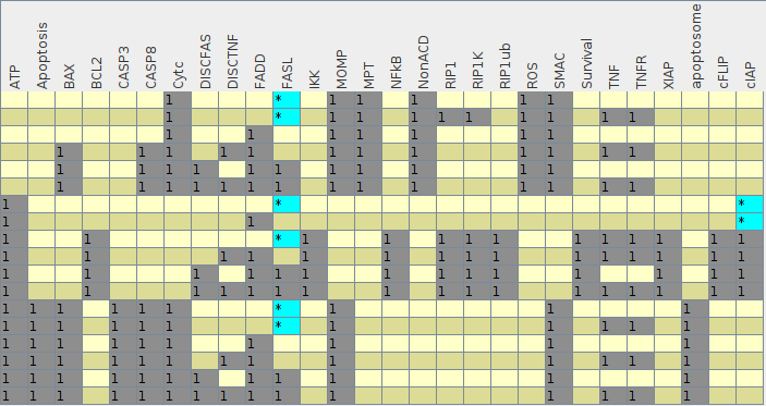
Figure 1: $27$ steady states of the complete BN computed with GINsim [21]. Components marked with * can either be set to zero or one. Steady states are grouped into phenotypes. Six steady states are not corresponding to any phenotype.

7 Possible further improvements

There is still some room for further improvement of the above algorithm. We address the third point in the beginning of 4. We can represent the lexicographical orderings on $\mathbb{B}(n)$ using weight vectors $w\in\mathbb{N}^{n}$. More precisely, let $\succ$ be any monomial ordering in $\mathbb{F}_{2}[x_{1},\dots,x_{n}]$ and $w\in\mathbb{N}^{n}$ any weight vector. Then we define $\succ_{w}$ as follows: for two monomials $x^{\alpha}$ and $x^{\beta}$, $\alpha,\beta\in\mathbb{N}^{n}$ we set

$$x^{\alpha}\succ_{w}x^{\beta}\Leftrightarrow w\cdot\alpha>w\cdot\beta\text{ or }(w\cdot\alpha=w\cdot\beta\text{ and }x^{\alpha}\succ x^{\beta})\cdot$$

According to [36, Prop 1.11] for every monomial ordering $\succ$ and for every ideal in $\mathbb{F}_{2}[x_{1},\dots,x_{n}]$ there exists a non-negative integer vector $w\in\mathbb{N}^{n}$ s.t. $in_{w}(\mathcal{I})=in_{\succ}(\mathcal{I})$ where $in_{w}(\mathcal{I})$ is the ideal generated by the initial forms $in_{w}(f),f\in\mathcal{I}$ –that is, the sum of monomials $x^{\alpha}$ in $f$ which are maximal with respect to the inner product $\alpha\cdot w$. We say also in this case $w$ represents $\succ$ for $\mathcal{I}$. The following lemma shows how we can construct weight vectors representing lexicographical orderings. Note that each ideal in $\mathbb{B}(n)$ is a principal ideal and each ideal $\langle f\rangle$ in $\mathbb{B}(n)$ corresponds to an ideal $\langle f,x_{1}^{2}+x_{1},\dots,x_{n}^{2}+x_{n}\rangle$ in $\mathbb{F}_{2}[x_{1},\dots,x_{n}]$. Let us also for simplicity consider the lexicographical ordering defined by $x_{n}\succ x_{n-1}\succ\cdots\succ x_{1}$. The general case can be obtained by permutation.

Lemma 7.1.

Consider an ideal of the form $\mathcal{I}=\langle f,x_{1}^{2}+x_{1},\dots,x_{n}^{2}+x_{n}\rangle\subseteq\mathbb{F}_{2}[x_{1},\dots,x_{n}]$ and the lexicographical ordering $\succ$ defined by $x_{n}\succ x_{n-1}\succ\cdots\succ x_{1}$. Then $\succ$ is represented by the weight vector $w\in\mathbb{Q}^{n}$ with $w_{k}=1+\sum_{j=1}^{k-1}w_{j}$ or alternatively $w_{k}=2^{k-1}$.

Proof.

Let $\succ$ be as above and $w$ the corresponding weight vector defined there. We first show that $in_{w}(\mathcal{I})\subseteq in_{\succ}(\mathcal{I})$. This is true since by definition of $\mathcal{I}$ we know that the monomials $x_{1}^{2},\dots,x_{n}^{2}$ are contained in $in_{w}(\mathcal{I})$ (and obviously in $in_{\succ}(\mathcal{I})$). Consequently, we can represent $in_{w}(\mathcal{I})$ in the form $in_{w}(\mathcal{I})=\langle in_{w}(g_{1}),\dots,in_{w}(g_{k}),x_{1}^{2},\dots,x_{n}^{2}\rangle$ with square free polynomials $g_{1},\dots,g_{k}$ in $\mathcal{I}$. Now by construction of $w$ for square free polynomials $g\in\mathbb{F}_{2}[x_{1},\dots,x_{n}]$ the equality $in_{w}(g)=in_{\succ}(g)$ holds. It follows $in_{w}(\mathcal{I})\subseteq in_{\succ}(\mathcal{I})$. Analogously it holds $in_{\succ}(\mathcal{I})\subseteq in_{w}(\mathcal{I})$. ∎

Let us call a reduced Gröbner basis with a distinguished initial monomial a marked Gröbner basis in accordance with [13, p. 428]. Next, we form equivalence classes of weight vectors which will lead to the same marked Gröbner bases.

Definition 7.1 ([13, p. 429]).

Let $G$ be any marked Gröbner basis for an ideal $\mathcal{I}$ consisting of $t$ polynomials

$$g_{i}=x^{\alpha(i)}+\sum_{\beta}c_{i,\beta}x^{\beta},$$

where $i\in\{1,\dots,t\}$ and $x^{\alpha(i)}$ is the initial monomial. We denote with $C_{G}$ the set

$$C_{G}=\big{\{}w\in(\mathbb{R}^{n})^{+}:(\alpha(i)-\beta)\cdot w\geq 0\text{ whenever }c_{i,\beta}\not=0\big{\}}.$$

We can combine 7.1 and 7.1 to potentially improve our algorithm. If we computed for a lexicographical ordering in 1 a Gröbner basis $G$ we can compute and save the equivalence class $C_{G}$. Now proceeding with the algorithm, for a new lexicographical ordering we need to check, we can create the corresponding weight vector $w$ using 7.1 and check if $w$ is in any of the previously computed equivalence classes $C_{G}$. If this is the case we can use the result of the previous computation.

Another aspect of the algorithm we can improve is the conversion of Gröbner bases. For an ideal $\mathcal{I}(B)=\langle f,x_{1}^{2}+x_{1},\dots,x_{n}^{2}+x_{n}\rangle$ the ring $\mathbb{F}_{2}[x_{1},\dots,x_{n}]\big{/}\mathcal{I}(B)$ is zero-dimensional, and so a finite dimensional vector space. Therefore, it is possible to use linear algebra for the conversion of Gröbner bases. This leads to the Faugère-Gianni-Lazard-Mora algorithm (FLGM algorithm) [16, 13, p. 49].

8 Conclusion

We reformulated 3.1 into the language of algebraic geometry. To do so we described the set of potential classifiers using residue classes modulo the vanishing ideal of the attractors or steady states of the Boolean network. This enabled us to construct an algorithm using normal forms to compute optimal classifiers. Subsequently we demonstrated the usefulness of this approach by creating an algorithm that produces the minimal solutions to 3.1. We showed that it is possible to apply this algorithm to a model for cell-fate decision with $25$ components from [8]. Especially, in combination with reduction algorithms for Boolean networks this allows us to investigate larger networks.

We hope that it will be also possible to exploit the algebraic reformulation further to speed up computations to tackle even larger networks. Some parts in the algorithm can be improved to obtain potentially faster computation times. For example the conversion between different Gröbner bases can be done more efficiently using the FLGM algorithm (see [16, 13, p. 49-54]) which uses linear algebra for the conversion of Gröbner bases. Since at the moment of writing this article there was no implementation of this available in PolyBoRi we did not use this potential improvement.

However, the main bottleneck for the speed of the algorithm seems to be the enumeration of possible orderings (or more precisely candidate sets). Therefore, we believe that this will not lead to a significant increase in speed but this remains to be tested. Instead we believe, that for larger networks heuristics should be investigated. Here ideas from the machine learning community could be useful. Potential crosslinks to classifications problems considered there should be explored in the future.

Also different optimality criteria for picking classifiers might be useful. For example one could try to attribute measurement costs to components and pick polynomial orderings which lead to optimal results in such a context as well.

In the introduction we mentioned the relationship of 3.1 to problems in the LAD community. There one starts typically with a data set of Boolean vectors. Here we focused on the case where our sets to be classifies are implicitly given. However, approaches developed for interpolation of Boolean polynomials from data points such as[6] could be used in the future to tailor our approach to such scenarios as well.

Appendix

Table 3: $9$ different representations of classifier for NonACD (see 6).

Components	Expression
$ATP$	$ATP+1$
$CASP3$, $Cytc$	$Cytc+CASP3$
$CASP3$, $MOMP$	$MOMP+CASP3$
$CASP3$, $SMAC$	$SMAC+CASP3$
$Cytc$, $apoptosome$	$Cytc+apoptosome$
$MOMP$, $apoptosome$	$apoptosome+MOMP$
$MPT$	$MPT$
$ROS$	$ROS$
$SMAC$, $apoptosome$	$apoptosome+SMAC$

Table 4: $17$ different representations of the classifier for apoptosis (see 6)

Components	Expression
$ATP,BAX$	$BAX\cdot ATP$
$ATP,CASP8$	$ATP\cdot CASP8$
$ATP,Cytc$	$Cytc+ATP+1$
$ATP,MOMP$	$ATP+MOMP+1$
$ATP,SMAC$	$ATP+SMAC+1$
$BAX,MPT$	$BAX\cdot MPT+BAX$
$BAX,ROS$	$BAX\cdot ROS+BAX$
$CASP3,$	$CASP3$
$CASP8,MPT$	$MPT\cdot CASP8+CASP8$
$CASP8,ROS$	$ROS\cdot CASP8+CASP8$
$Cytc,MPT$	$Cytc+MPT$
$Cytc,ROS$	$Cytc+ROS$
$MOMP,MPT$	$MPT+MOMP$
$MOMP,ROS$	$ROS+MOMP$
$MPT,SMAC$	$MPT+SMAC$
$ROS,SMAC$	$ROS+SMAC$
$apoptosome,$	$apoptosome$

Table 5: 84 different representations of the classifier of survival of the cell. (see Section 6)

Components	Expression
$ATP$, $BAX$, $DISCFAS$, $TNF$	$DISCFAS\cdot BAX+DISCFAS\cdot ATP+DISCFAS\cdot TNF+BAX\cdot ATP+BAX\cdot TNF+BAX+ATP\cdot TNF$
$ATP$, $BAX$, $DISCFAS$, $TNFR$	$DISCFAS\cdot BAX+DISCFAS\cdot ATP+DISCFAS\cdot TNFR+BAX\cdot ATP+BAX\cdot TNFR+BAX+ATP\cdot TNFR$
$ATP$, $BAX$, $FADD$, $FASL$, $TNF$	$BAX\cdot FASL\cdot FADD+BAX\cdot TNF+ATP\cdot FASL\cdot FADD\cdot TNF+ATP\cdot FADD\cdot TNF+ATP\cdot TNF+FASL\cdot FADD+FADD\cdot TNF$
$ATP$, $BAX$, $FADD$, $FASL$, $TNFR$	$BAX\cdot TNFR+BAX\cdot FASL\cdot FADD+ATP\cdot TNFR\cdot FASL\cdot FADD+ATP\cdot TNFR\cdot FADD+ATP\cdot TNFR+TNFR\cdot FADD+FASL\cdot FADD$
$ATP$, $CASP3$, $DISCFAS$, $TNF$	$DISCFAS\cdot ATP\cdot TNF+DISCFAS\cdot ATP+DISCFAS\cdot CASP3+ATP\cdot TNF+TNF\cdot CASP3$
$ATP$, $CASP3$, $DISCFAS$, $TNFR$	$DISCFAS\cdot ATP\cdot TNFR+DISCFAS\cdot ATP+DISCFAS\cdot CASP3+ATP\cdot TNFR+TNFR\cdot CASP3$
$ATP$, $CASP3$, $FADD$, $FASL$, $TNF$	$ATP\cdot FASL\cdot FADD\cdot TNF+ATP\cdot FASL\cdot FADD+ATP\cdot TNF+FASL\cdot FADD\cdot CASP3+TNF\cdot CASP3$
$ATP$, $CASP3$, $FADD$, $FASL$, $TNFR$	$ATP\cdot TNFR\cdot FASL\cdot FADD+ATP\cdot TNFR+ATP\cdot FASL\cdot FADD+TNFR\cdot CASP3+FASL\cdot FADD\cdot CASP3$
$ATP$, $CASP8$, $DISCFAS$, $TNF$	$DISCFAS\cdot TNF\cdot CASP8+DISCFAS\cdot TNF+DISCFAS\cdot CASP8+DISCFAS+ATP\cdot TNF\cdot CASP8+ATP\cdot TNF$
$ATP$, $CASP8$, $DISCFAS$, $TNFR$	$DISCFAS\cdot TNFR\cdot CASP8+DISCFAS\cdot TNFR+DISCFAS\cdot CASP8+DISCFAS+ATP\cdot TNFR\cdot CASP8+ATP\cdot TNFR$
$ATP$, $CASP8$, $FADD$, $FASL$, $TNF$	$ATP\cdot TNF\cdot CASP8+ATP\cdot TNF+FASL\cdot FADD\cdot TNF\cdot CASP8+FASL\cdot FADD\cdot TNF+FASL\cdot FADD\cdot CASP8+FASL\cdot FADD$
$ATP$, $CASP8$, $FADD$, $FASL$, $TNFR$	$ATP\cdot TNFR+ATP\cdot FASL\cdot CASP8+ATP\cdot CASP8+TNFR\cdot FASL\cdot FADD+TNFR\cdot CASP8+FASL\cdot FADD\cdot CASP8+FASL\cdot FADD+FASL\cdot CASP8+CASP8$
$ATP$, $DISCFAS$, $TNF$, $apoptosome$	$DISCFAS\cdot ATP\cdot TNF+DISCFAS\cdot ATP+DISCFAS\cdot apoptosome+ATP\cdot TNF+apoptosome\cdot TNF$
$ATP$, $DISCFAS$, $TNFR$, $apoptosome$	$DISCFAS\cdot ATP\cdot TNFR+DISCFAS\cdot ATP+DISCFAS\cdot apoptosome+ATP\cdot TNFR+apoptosome\cdot TNFR$
$ATP$, $FADD$, $FASL$, $TNF$, $apoptosome$	$ATP\cdot FASL\cdot FADD\cdot TNF+ATP\cdot FASL\cdot FADD+ATP\cdot TNF+apoptosome\cdot FASL\cdot FADD+apoptosome\cdot TNF$
$ATP$, $FADD$, $FASL$, $TNFR$, $apoptosome$	$ATP\cdot TNFR\cdot FASL\cdot FADD+ATP\cdot TNFR+ATP\cdot FASL\cdot FADD+apoptosome\cdot TNFR+apoptosome\cdot FASL\cdot FADD$
$ATP$, $RIP1$	$ATP\cdot RIP1$
$ATP$, $RIP1K$	$ATP\cdot RIP1K$
$BAX$, $DISCFAS$, $MPT$, $TNF$	$DISCFAS\cdot BAX+DISCFAS\cdot MPT+DISCFAS\cdot TNF+DISCFAS+BAX\cdot MPT+BAX\cdot TNF+MPT\cdot TNF+TNF$
$BAX$, $DISCFAS$, $MPT$, $TNFR$	$DISCFAS\cdot BAX+DISCFAS\cdot TNFR+DISCFAS\cdot MPT+DISCFAS+BAX\cdot TNFR+BAX\cdot MPT+TNFR\cdot MPT+TNFR$
$BAX$, $DISCFAS$, $ROS$, $TNF$	$DISCFAS\cdot BAX+DISCFAS\cdot ROS+DISCFAS\cdot TNF+DISCFAS+BAX\cdot ROS+BAX\cdot TNF+ROS\cdot TNF+TNF$
$BAX$, $DISCFAS$, $ROS$, $TNFR$	$DISCFAS\cdot BAX+DISCFAS\cdot TNFR+DISCFAS\cdot ROS+DISCFAS+BAX\cdot TNFR+BAX\cdot ROS+TNFR\cdot ROS+TNFR$
$BAX$, $FADD$, $FASL$, $MPT$, $TNF$	$BAX\cdot FASL\cdot FADD+BAX\cdot TNF+MPT\cdot FASL\cdot FADD\cdot TNF+MPT\cdot FADD\cdot TNF+MPT\cdot TNF+FASL\cdot FADD\cdot TNF+FASL\cdot FADD+TNF$
$BAX$, $FADD$, $FASL$, $MPT$, $TNFR$	$BAX\cdot TNFR+BAX\cdot FASL\cdot FADD+TNFR\cdot MPT\cdot FASL\cdot FADD+TNFR\cdot MPT\cdot FADD+TNFR\cdot MPT+TNFR\cdot FASL\cdot FADD+TNFR+FASL\cdot FADD$
$BAX$, $FADD$, $FASL$, $ROS$, $TNF$	$BAX\cdot FASL\cdot FADD+BAX\cdot TNF+FASL\cdot FADD\cdot ROS\cdot TNF+FASL\cdot FADD\cdot TNF+FASL\cdot FADD+FADD\cdot ROS\cdot TNF+ROS\cdot TNF+TNF$
$BAX$, $FADD$, $FASL$, $ROS$, $TNFR$	$BAX\cdot TNFR+BAX\cdot FASL\cdot FADD+TNFR\cdot FASL\cdot FADD\cdot ROS+TNFR\cdot FASL\cdot FADD+TNFR\cdot FADD\cdot ROS+TNFR\cdot ROS+TNFR+FASL\cdot FADD$
$BCL2$	$BCL2$
$CASP3$, $DISCFAS$, $MPT$, $TNF$	$DISCFAS\cdot MPT\cdot TNF+DISCFAS\cdot MPT+DISCFAS\cdot TNF+DISCFAS\cdot CASP3+DISCFAS+MPT\cdot TNF+TNF\cdot CASP3+TNF$
$CASP3$, $DISCFAS$, $MPT$, $TNFR$	$DISCFAS\cdot TNFR\cdot MPT+DISCFAS\cdot TNFR+DISCFAS\cdot MPT+DISCFAS\cdot CASP3+DISCFAS+TNFR\cdot MPT+TNFR\cdot CASP3+TNFR$
$CASP3$, $DISCFAS$, $ROS$, $TNF$	$DISCFAS\cdot ROS\cdot TNF+DISCFAS\cdot ROS+DISCFAS\cdot TNF+DISCFAS\cdot CASP3+DISCFAS+ROS\cdot TNF+TNF\cdot CASP3+TNF$
$CASP3$, $DISCFAS$, $ROS$, $TNFR$	$DISCFAS\cdot TNFR\cdot ROS+DISCFAS\cdot TNFR+DISCFAS\cdot ROS+DISCFAS\cdot CASP3+DISCFAS+TNFR\cdot ROS+TNFR\cdot CASP3+TNFR$
$CASP3$, $FADD$, $FASL$, $MPT$, $TNF$	$MPT\cdot FASL\cdot FADD\cdot TNF+MPT\cdot FASL\cdot FADD+MPT\cdot TNF+FASL\cdot FADD\cdot TNF+FASL\cdot FADD\cdot CASP3+FASL\cdot FADD+TNF\cdot CASP3+TNF$
$CASP3$, $FADD$, $FASL$, $MPT$, $TNFR$	$TNFR\cdot MPT\cdot FASL\cdot FADD+TNFR\cdot MPT+TNFR\cdot FASL\cdot FADD+TNFR\cdot CASP3+TNFR+MPT\cdot FASL\cdot FADD+FASL\cdot FADD\cdot CASP3+FASL\cdot FADD$
$CASP3$, $FADD$, $FASL$, $ROS$, $TNF$	$FASL\cdot FADD\cdot ROS\cdot TNF+FASL\cdot FADD\cdot ROS+FASL\cdot FADD\cdot TNF+FASL\cdot FADD\cdot CASP3+FASL\cdot FADD+ROS\cdot TNF+TNF\cdot CASP3+TNF$
$CASP3$, $FADD$, $FASL$, $ROS$, $TNFR$	$TNFR\cdot FASL\cdot FADD\cdot ROS+TNFR\cdot FASL\cdot FADD+TNFR\cdot ROS+TNFR\cdot CASP3+TNFR+FASL\cdot FADD\cdot ROS+FASL\cdot FADD\cdot CASP3+FASL\cdot FADD$
$CASP8$, $DISCFAS$, $MPT$, $TNF$	$DISCFAS\cdot TNF\cdot CASP8+DISCFAS\cdot TNF+DISCFAS\cdot CASP8+DISCFAS+MPT\cdot TNF\cdot CASP8+MPT\cdot TNF+TNF\cdot CASP8+TNF$
$CASP8$, $DISCFAS$, $MPT$, $TNFR$	$DISCFAS\cdot TNFR+DISCFAS\cdot MPT+DISCFAS\cdot CASP8+DISCFAS+TNFR\cdot MPT+TNFR\cdot CASP8+TNFR+MPT\cdot CASP8$
$CASP8$, $DISCFAS$, $ROS$, $TNF$	$DISCFAS\cdot TNF\cdot CASP8+DISCFAS\cdot TNF+DISCFAS\cdot CASP8+DISCFAS+ROS\cdot TNF\cdot CASP8+ROS\cdot TNF+TNF\cdot CASP8+TNF$
$CASP8$, $DISCFAS$, $ROS$, $TNFR$	$DISCFAS\cdot TNFR+DISCFAS\cdot ROS+DISCFAS\cdot CASP8+DISCFAS+TNFR\cdot ROS+TNFR\cdot CASP8+TNFR+ROS\cdot CASP8$
$CASP8$, $FADD$, $FASL$, $MPT$, $TNF$	$MPT\cdot TNF\cdot CASP8+MPT\cdot TNF+FASL\cdot FADD\cdot TNF\cdot CASP8+FASL\cdot FADD\cdot TNF+FASL\cdot FADD\cdot CASP8+FASL\cdot FADD+TNF\cdot CASP8+TNF$
$CASP8$, $FADD$, $FASL$, $MPT$, $TNFR$	$TNFR\cdot MPT+TNFR\cdot FASL\cdot FADD+TNFR\cdot CASP8+TNFR+MPT\cdot FASL\cdot CASP8+MPT\cdot CASP8+FASL\cdot FADD\cdot CASP8+FASL\cdot FADD$
$CASP8$, $FADD$, $FASL$, $ROS$, $TNF$	$FASL\cdot FADD\cdot TNF+FASL\cdot FADD\cdot CASP8+FASL\cdot FADD+FASL\cdot ROS\cdot CASP8+ROS\cdot TNF+ROS\cdot CASP8+TNF\cdot CASP8+TNF$
$CASP8$, $FADD$, $FASL$, $ROS$, $TNFR$	$TNFR\cdot FASL\cdot FADD+TNFR\cdot ROS+TNFR\cdot CASP8+TNFR+FASL\cdot FADD\cdot CASP8+FASL\cdot FADD+FASL\cdot ROS\cdot CASP8+ROS\cdot CASP8$
$Cytc$, $DISCFAS$, $TNF$	$Cytc\cdot DISCFAS\cdot TNF+Cytc\cdot DISCFAS+Cytc\cdot TNF+DISCFAS\cdot TNF+DISCFAS+TNF$
$Cytc$, $DISCFAS$, $TNFR$	$Cytc\cdot DISCFAS\cdot TNFR+Cytc\cdot DISCFAS+Cytc\cdot TNFR+DISCFAS\cdot TNFR+DISCFAS+TNFR$
$Cytc$, $FADD$, $FASL$, $TNF$	$Cytc\cdot FASL\cdot FADD\cdot TNF+Cytc\cdot FASL\cdot FADD+Cytc\cdot TNF+FASL\cdot FADD\cdot TNF+FASL\cdot FADD+TNF$
$Cytc$, $FADD$, $FASL$, $TNFR$	$Cytc\cdot TNFR\cdot FASL\cdot FADD+Cytc\cdot TNFR+Cytc\cdot FASL\cdot FADD+TNFR\cdot FASL\cdot FADD+TNFR+FASL\cdot FADD$
$Cytc$, $RIP1$	$Cytc\cdot RIP1+RIP1$
$Cytc$, $RIP1K$	$Cytc\cdot RIP1K+RIP1K$
$DISCFAS$, $MOMP$, $TNF$	$DISCFAS\cdot MOMP\cdot TNF+DISCFAS\cdot MOMP+DISCFAS\cdot TNF+DISCFAS+MOMP\cdot TNF+TNF$
$DISCFAS$, $MOMP$, $TNFR$	$DISCFAS\cdot TNFR\cdot MOMP+DISCFAS\cdot TNFR+DISCFAS\cdot MOMP+DISCFAS+TNFR\cdot MOMP+TNFR$
$DISCFAS$, $MPT$, $TNF$, $apoptosome$	$DISCFAS\cdot apoptosome+DISCFAS\cdot MPT\cdot TNF+DISCFAS\cdot MPT+DISCFAS\cdot TNF+DISCFAS+apoptosome\cdot TNF+MPT\cdot TNF+TNF$
$DISCFAS$, $MPT$, $TNFR$, $apoptosome$	$DISCFAS\cdot apoptosome+DISCFAS\cdot TNFR\cdot MPT+DISCFAS\cdot TNFR+DISCFAS\cdot MPT+DISCFAS+apoptosome\cdot TNFR+TNFR\cdot MPT+TNFR$
$DISCFAS$, $ROS$, $TNF$, $apoptosome$	$DISCFAS\cdot apoptosome+DISCFAS\cdot ROS\cdot TNF+DISCFAS\cdot ROS+DISCFAS\cdot TNF+DISCFAS+apoptosome\cdot TNF+ROS\cdot TNF+TNF$
$DISCFAS$, $ROS$, $TNFR$, $apoptosome$	$DISCFAS\cdot apoptosome+DISCFAS\cdot TNFR\cdot ROS+DISCFAS\cdot TNFR+DISCFAS\cdot ROS+DISCFAS+apoptosome\cdot TNFR+TNFR\cdot ROS+TNFR$
$DISCFAS$, $SMAC$, $TNF$	$DISCFAS\cdot SMAC\cdot TNF+DISCFAS\cdot SMAC+DISCFAS\cdot TNF+DISCFAS+SMAC\cdot TNF+TNF$
$DISCFAS$, $SMAC$, $TNFR$	$DISCFAS\cdot TNFR\cdot SMAC+DISCFAS\cdot TNFR+DISCFAS\cdot SMAC+DISCFAS+TNFR\cdot SMAC+TNFR$
$DISCFAS$, $TNF$, $cIAP$	$DISCFAS\cdot TNF\cdot cIAP+DISCFAS\cdot cIAP+TNF\cdot cIAP$
$DISCFAS$, $TNFR$, $cIAP$	$DISCFAS\cdot TNFR\cdot cIAP+DISCFAS\cdot cIAP+TNFR\cdot cIAP$
$FADD$, $FASL$, $MOMP$, $TNF$	$FASL\cdot FADD\cdot MOMP\cdot TNF+FASL\cdot FADD\cdot MOMP+FASL\cdot FADD\cdot TNF+FASL\cdot FADD+MOMP\cdot TNF+TNF$
$FADD$, $FASL$, $MOMP$, $TNFR$	$TNFR\cdot FASL\cdot FADD\cdot MOMP+TNFR\cdot FASL\cdot FADD+TNFR\cdot MOMP+TNFR+FASL\cdot FADD\cdot MOMP+FASL\cdot FADD$
$FADD$, $FASL$, $MPT$, $TNF$, $apoptosome$	$apoptosome\cdot FASL\cdot FADD+apoptosome\cdot TNF+MPT\cdot FASL\cdot FADD\cdot TNF+MPT\cdot FASL\cdot FADD+MPT\cdot TNF+FASL\cdot FADD\cdot TNF+FASL\cdot FADD+TNF$
$FADD$, $FASL$, $MPT$, $TNFR$, $apoptosome$	$apoptosome\cdot TNFR+apoptosome\cdot FASL\cdot FADD+TNFR\cdot MPT\cdot FASL\cdot FADD+TNFR\cdot MPT+TNFR\cdot FASL\cdot FADD+TNFR+MPT\cdot FASL\cdot FADD+FASL\cdot FADD$
$FADD$, $FASL$, $ROS$, $TNF$, $apoptosome$	$apoptosome\cdot FASL\cdot FADD+apoptosome\cdot TNF+FASL\cdot FADD\cdot ROS\cdot TNF+FASL\cdot FADD\cdot ROS+FASL\cdot FADD\cdot TNF+FASL\cdot FADD+ROS\cdot TNF+TNF$
$FADD$, $FASL$, $ROS$, $TNFR$, $apoptosome$	$apoptosome\cdot TNFR+apoptosome\cdot FASL\cdot FADD+TNFR\cdot FASL\cdot FADD\cdot ROS+TNFR\cdot FASL\cdot FADD+TNFR\cdot ROS+TNFR+FASL\cdot FADD\cdot ROS+FASL\cdot FADD$
$FADD$, $FASL$, $SMAC$, $TNF$	$FASL\cdot FADD\cdot SMAC\cdot TNF+FASL\cdot FADD\cdot SMAC+FASL\cdot FADD\cdot TNF+FASL\cdot FADD+SMAC\cdot TNF+TNF$
$FADD$, $FASL$, $SMAC$, $TNFR$	$TNFR\cdot FASL\cdot FADD\cdot SMAC+TNFR\cdot FASL\cdot FADD+TNFR\cdot SMAC+TNFR+FASL\cdot FADD\cdot SMAC+FASL\cdot FADD$
$FADD$, $FASL$, $TNF$, $cIAP$	$FASL\cdot FADD\cdot TNF\cdot cIAP+FASL\cdot FADD\cdot cIAP+TNF\cdot cIAP$
$FADD$, $FASL$, $TNFR$, $cIAP$	$TNFR\cdot FASL\cdot FADD\cdot cIAP+TNFR\cdot cIAP+FASL\cdot FADD\cdot cIAP$
$IKK$	$IKK$
$MOMP$, $RIP1$	$MOMP\cdot RIP1+RIP1$
$MOMP$, $RIP1K$	$RIP1K\cdot MOMP+RIP1K$
$MPT$, $RIP1$	$MPT\cdot RIP1+RIP1$
$MPT$, $RIP1K$	$RIP1K\cdot MPT+RIP1K$
$NFKB1$	$NFKB1$
$RIP1$, $ROS$	$ROS\cdot RIP1+RIP1$
$RIP1$, $SMAC$	$SMAC\cdot RIP1+RIP1$
$RIP1$, $cIAP$	$RIP1\cdot cIAP$
$RIP1K$, $ROS$	$RIP1K\cdot ROS+RIP1K$
$RIP1K$, $SMAC$	$RIP1K\cdot SMAC+RIP1K$
$RIP1K$, $cIAP$	$RIP1K\cdot cIAP$
$RIP1ub$	$RIP1ub$
$XIAP$	$XIAP$
$cFLIP$	$cFLIP$

References

• [1] Albert, R., Thakar, J.: Boolean modeling: a logic-based dynamic approach for understanding signaling and regulatory networks and for making useful predictions. Wiley Interdisciplinary Reviews: Systems Biology and Medicine 6(5), 353–369 (2014)
• [2] Alexe, S., Blackstone, E., Hammer, P.L., Ishwaran, H., Lauer, M.S., Snader, C.E.P.: Coronary risk prediction by logical analysis of data. Annals of Operations Research 119(1-4), 15–42 (2003)
• [3] Bonzanni, N., Garg, A., Feenstra, K.A., Schütte, J., Kinston, S., Miranda-Saavedra, D., Heringa, J., Xenarios, I., Göttgens, B.: Hard-wired heterogeneity in blood stem cells revealed using a dynamic regulatory network model. Bioinformatics 29(13), i80–i88 (2013)
• [4] Boros, E., Hammer, P.L., Ibaraki, T., Kogan, A., Mayoraz, E., Muchnik, I.: An implementation of logical analysis of data. IEEE Transactions on knowledge and Data Engineering 12(2), 292–306 (2000)
• [5] Brickenstein, M., Dreyer, A.: Polybori: A framework for gröbner-basis computations with Boolean polynomials. Journal of Symbolic Computation 44(9), 1326–1345 (2009)
• [6] Brickenstein, M., Dreyer, A.: Gröbner-free normal forms for Boolean polynomials. Journal of Symbolic Computation (2013)
• [7] Buchberger, B.: Applications of Gröbner Bases in Non-Linear Computational Geometry. In: Rice, J.R. (ed.) Mathematical Aspects of Scientific Software, pp. 59–87. The IMA Volumes in Mathematics and Its Applications, Springer, New York, NY (1988), https://doi.org/10.1007/978-1-4684-7074-1˙3
• [8] Calzone, L., Tournier, L., Fourquet, S., Thieffry, D., Zhivotovsky, B., Barillot, E., Zinovyev, A.: Mathematical modelling of cell-fate decision in response to death receptor engagement. PLOS Computational Biology 6(3), 1–15 (03 2010). https://doi.org/10.1371/journal.pcbi.1000702, https://doi.org/10.1371/journal.pcbi.1000702
• [9] Chaouiya, C., Remy, E., Mossé, B., Thieffry, D.: Qualitative analysis of regulatory graphs: a computational tool based on a discrete formal framework. In: Positive systems, pp. 119–126. Springer (2003)
• [10] Cheng, D., Qi, H.: Controllability and observability of boolean control networks. Automatica 45(7), 1659–1667 (2009)
• [11] Chikalov, I., Lozin, V., Lozina, I., Moshkov, M., Nguyen, H.S., Skowron, A., Zielosko, B.: Logical analysis of data: Theory, methodology and applications. In: Three approaches to data analysis, pp. 147–192. Springer (2013)
• [12] Cox, D., Little, J., O’shea, D.: Ideals, varieties, and algorithms, vol. 3. Springer (2007)
• [13] Cox, D.A., Little, J., O’Shea, D.: Using Algebraic Geometry. Graduate Texts in Mathematics, Springer-Verlag (2004)
• [14] Dickenstein, A., Millán, M.P., Shiu, A., Tang, X.: Multistationarity in Structured Reaction Networks. Bulletin of Mathematical Biology 81(5), 1527–1581 (May 2019). https://doi.org/10.1007/s11538-019-00572-6, https://doi.org/10.1007/s11538-019-00572-6
• [15] Drton, M., Sturmfels, B., Sullivant, S.: Lectures on Algebraic Statistics. Oberwolfach Seminars, Birkhäuser Basel (2009), https://www.springer.com/gp/book/9783764389048
• [16] Faugère, J.C., Gianni, P., Lazard, D., Mora, T.: Efficient computation of zero-dimensional gröbner bases by change of ordering. Journal of Symbolic Computation 16(4), 329–344 (1993)
• [17] Faugère, J.C., Joux, A.: Algebraic Cryptanalysis of Hidden Field Equation (HFE) Cryptosystems Using Gröbner Bases. In: Boneh, D. (ed.) Advances in Cryptology - CRYPTO 2003. pp. 44–60. Lecture Notes in Computer Science, Springer, Berlin, Heidelberg (2003)
• [18] Fauré, A., Vreede, B.M., Sucena, É., Chaouiya, C.: A discrete model of drosophila eggshell patterning reveals cell-autonomous and juxtacrine effects. PLoS computational biology 10(3), e1003527 (2014)
• [19] Gao, S., Platzer, A., Clarke, E.M.: Quantifier elimination over finite fields using Gröbner bases. In: Winkler, F. (ed.) Algebraic Informatics. pp. 140–157. Springer Berlin Heidelberg, Berlin, Heidelberg (2011)
• [20] Germundsson, R.: Basic results on ideals and varieties in finite fields. Tech. Rep. S-581 83 (1991)
• [21] Gonzalez, A.G., Naldi, A., Sánchez, L., Thieffry, D., Chaouiya, C.: GINsim: A software suite for the qualitative modelling, simulation and analysis of regulatory networks. Biosystems 84(2), 91 – 100 (2006). https://doi.org/https://doi.org/10.1016/j.biosystems.2005.10.003, http://www.sciencedirect.com/science/article/pii/S0303264705001693, dynamical Modeling of Biological Regulatory Networks
• [22] González, A., Chaouiya, C., Thieffry, D.: Logical modelling of the role of the hh pathway in the patterning of the drosophila wing disc. Bioinformatics 24(16), i234–i240 (2008)
• [23] Hammer, P.L., Bonates, T.O.: Logical analysis of data - an overview: From combinatorial optimization to medical applications. Annals of Operations Research 148(1), 203–225 (2006)
• [24] Jarrah, A.S., Laubenbacher, R.: Discrete models of biochemical networks: The toric variety of nested canalyzing functions. In: International Conference on Algebraic Biology. pp. 15–22. Springer (2007)
• [25] Laubenbacher, R., Stigler, B.: A computational algebra approach to the reverse engineering of gene regulatory networks. Journal of Theoretical Biology 229(4), 523 – 537 (2004). https://doi.org/https://doi.org/10.1016/j.jtbi.2004.04.037, http://www.sciencedirect.com/science/article/pii/S0022519304001754
• [26] Le Novere, N.: Quantitative and logic modelling of molecular and gene networks. Nature Reviews Genetics 16(3), 146–158 (2015)
• [27] Millán, M.P., Dickenstein, A., Shiu, A., Conradi, C.: Chemical reaction systems with toric steady states. Bulletin of mathematical biology 74(5), 1027–1065 (2012)
• [28] Minato, S.i.: Zero-suppressed bdds for set manipulation in combinatorial problems. In: Proceedings of the 30th international Design Automation Conference. pp. 272–277. ACM (1993)
• [29] Mishchenko, A.: An introduction to zero-suppressed binary decision diagrams. In: Proceedings of the 12th Symposium on the Integration of Symbolic Computation and Mechanized Reasoning. vol. 8, pp. 1–15. Citeseer (2001)
• [30] Murrugarra, D., Veliz-Cuba, A., Aguilar, B., Laubenbacher, R.: Identification of control targets in Boolean molecular network models via computational algebra. BMC Systems Biology 10(1),  94 (Sep 2016). https://doi.org/10.1186/s12918-016-0332-x, https://doi.org/10.1186/s12918-016-0332-x
• [31] Naldi, A., Remy, É., Thieffry, D., Chaouiya, C.: Dynamically consistent reduction of logical regulatory graphs. Theoretical Computer Science 412(21), 2207 – 2218 (2011). https://doi.org/https://doi.org/10.1016/j.tcs.2010.10.021, http://www.sciencedirect.com/science/article/pii/S0304397510005839, selected Papers from the 7th International Conference on Computational Methods in Systems Biology
• [32] Samaga, R., Klamt, S.: Modeling approaches for qualitative and semi-quantitative analysis of cellular signaling networks. Cell communication and signaling 11(1),  43 (2013)
• [33] Samaga, R., Saez-Rodriguez, J., Alexopoulos, L.G., Sorger, P.K., Klamt, S.: The logic of egfr/erbb signaling: theoretical properties and analysis of high-throughput data. PLoS computational biology 5(8), e1000438 (2009)
• [34] Sánchez, L., Chaouiya, C., Thieffry, D.: Segmenting the fly embryo: logical analysis of the role of the segment polarity cross-regulatory module. International journal of developmental biology 52(8), 1059–1075 (2002)
• [35] Sato, Y., Inoue, S., Suzuki, A., Nabeshima, K., Sakai, K.: Boolean gröbner bases. Journal of symbolic computation 46(5), 622–632 (2011)
• [36] Sturmfels, B.: Gröbner bases and convex polytopes, vol. 8. American Mathematical Soc. (1996)
• [37] Thobe, K., Sers, C., Siebert, H.: Unraveling the regulation of mtorc2 using logical modeling. Cell Communication and Signaling 15(1),  6 (2017)
• [38] Veliz-Cuba, A.: An algebraic approach to reverse engineering finite dynamical systems arising from biology. SIAM Journal on Applied Dynamical Systems 11(1), 31–48 (2012)
• [39] Veliz-Cuba, A., Aguilar, B., Hinkelmann, F., Laubenbacher, R.: Steady state analysis of Boolean molecular network models via model reduction and computational algebra. BMC Bioinformatics 15(1),  221 (Jun 2014). https://doi.org/10.1186/1471-2105-15-221, https://doi.org/10.1186/1471-2105-15-221
• [40] Veliz-Cuba, A., Jarrah, A.S., Laubenbacher, R.: Polynomial algebra of discrete models in systems biology. Bioinformatics 26(13), 1637–1643 (2010). https://doi.org/10.1093/bioinformatics/btq240, http://dx.doi.org/10.1093/bioinformatics/btq240
• [41] Vera-Licona, P., Jarrah, A., Garcia-Puente, L.D., McGee, J., Laubenbacher, R.: An algebra-based method for inferring gene regulatory networks. BMC systems biology 8(1),  37 (2014)