A Nested Cross Decomposition Algorithm for Power System Capacity Expansion with Multiscale Uncertainties

Abstract

Modern electric power systems have witnessed rapidly increasing penetration of renewable energy, storage, electrical vehicles and various demand response resources. The electric infrastructure planning is thus facing more challenges due to the variability and uncertainties arising from the diverse new resources. This study aims to develop a multistage and multiscale stochastic mixed integer programming (MM-SMIP) model to capture both the coarse-temporal-scale uncertainties, such as investment cost and long-run demand stochasticity, and fine-temporal-scale uncertainties, such as hourly renewable energy output and electricity demand uncertainties, for the power system capacity expansion problem. To be applied to a real power system, the resulting model will lead to extremely large-scale mixed integer programming problems, which suffer not only the well-known curse of dimensionality, but also computational difficulties with a vast number of integer variables at each stage. In addressing such challenges associated with the MM-SMIP model, we propose a nested cross decomposition algorithm that consists of two layers of decomposition, that is, the Dantzig-Wolfe decomposition and L-shaped decomposition. The algorithm exhibits promising computational performance under our numerical study, and is especially amenable to parallel computing, which will also be demonstrated through the computational results.

1 Introduction

Global electricity consumption is increasing rapidly because of economic growth and rising population. It is forecasted by the U.S. Energy Information Administration that the electricity use will grow by nearly 80% between 2018 and 2050 (US-EIA 2019). This makes it necessary to expand generation capacity so as to meet future electricity demand. Meanwhile, various renewable energy sources, including solar, wind and hydroelectric, and new clean technologies have emerged in the past decade to reduce air pollutant emissions and to promote sustainability. Environmental regulations have led the electric industry to retire aging fossil fuel generators and to build more and more power plants with these new technologies (Huang and Zheng 2020). Along with more installed generators, the expansion of transmission capacity might be necessary to mitigate power system congestion. Especially for wind farms which are usually located in sparsely-populated areas, new transmission lines are needed to connect the generation resources and demand centers. Furthermore, energy storage technologies can be installed and used as a buffer between generation and consumption, thereby mitigating the unpredictability and intermittency associated with renewable sources.

The capacity expansion of power system infrastrues is a capital-intensive and long-lasting process. However, few existing models truly integrate the planning of generation, transmission and energy storage over a long planning horizon due to computational complexities, although the coordinated planning may produce more cost effective results than a separate or sequential decision process (Krishnan et al. 2016). This motivates our work that co-optimizes all of the infrastructures and can be applied to large-scale systems through algorithm advances and high-performance computing. In addition to its aging infrastructures, the electricity sector in a power system is usually facing a rising amount of volatility in different time scales. In the coarse temporal scale, the capital costs for new installations and long-run electricity demand growth rates are both uncertain and can only be estimated. In the fine temporal scale, the intermittent nature of renewable energy poses considerable challenges to system operation as electricity supply and demand must be balanced at all times to ensure system reliability; and on the demand side, high penetration of plug-in electric vehicles and other demand response resources make future demand more unpredictable. These uncertainties need to be properly accounted for through the capacity expansion process, as otherwise the decisions might be either not cost minimizing or not sufficiently reliable to meet future demand (Lara et al. 2018, Liu et al. 2018). The need for a model with a multiscale structure that can produce a uniform infrastructure expansion schedule to accommodate a wide range of possibilities in the future provides another motivation for our study.

This paper proposes a multistage and multiscale stochastic mixed integer programming (MM-SMIP) model for the power system capacity expansion problem. The model is multistage in terms that it makes capacity expansion decisions in different stages of time; and at a given stage, with all the past uncertainties realized, it seeks the best planning decisions subject to future uncertainties of investment costs and electricity demand. It is multiscale in the sense that it integrates detalied short-term unit commitment modeling through the planning process with the consideration of uncertainties in the fine temporal scale, such as renewable energy output intermittency and hour-to-hour electricity demand volatility, in addition to those in the coarse temporal scale. The resulting model is an extremely large-scale stochastic mixed-integer program, easily of multi-million variables and constraints when applied to a real-world system. The multistage and multiscale features of the model, however, make it highly structured and decomposable. We propose a nested cross decomposition (NCD) algorithm to fully exploit such features, which is also amenable to parallel computing. There are two layers of decomposition for this problem. At the capacity expansion level, column generation is used to decompose the multistage expansion problem and iteratively generates feasible expansion plans. The second layer of L-shaped decomposition is to separate the stochastic unit commitment problems from the scenario tree of the expansion planning through cutting plane approximation. Even though we can decompose the huge MM-SMIP into much smaller problems, there are still a vast number of them. We employ parallel computing here as the decomposed problems can be solved independently.

The remainder of this paper is organized as follows. A literature review is provided in Section 2. Section 3 introduces the structure and mathematical formulation of the MM-SMIP model. Section 4 discusses the NCD algorithm for the proposed model. Numerical studies on the model and parallel computing implementation of the algorithm are presented in Section 5. Section 6 concludes the papers and discusses future research.

2 Literature Review

A planning process of capacity expansion is to identify infrastructure needs for a system to serve growing demand in the future. There is an extensive literature on capacity expansion and long-term planning in general (Luss 1982, Davis et al. 1987, Bean et al. 1992, Li and Tirupati 1994, Rajagopalan et al. 1998, Ahmed et al. 2003, Singh et al. 2009) and specific applications, such as communication networks (Laguna 1998, Riis and Andersen 2002), supply chain management (Santoso et al. 2005), project management (Conejo et al. 2021), manufacturing industries (Eppen et al. 1989, Sahinidis and Grossmann 1992) and service industries (Herman and Ganz 1994, Jena et al. 2017).

Planning for capacity expansion in an electric power system differs from the other applications, mainly because of various uncertainties from diverse resources and many requirements and constraints (e.g., ramping and minimum-up and down time constraints) for securing power syste operations. Stochastic optimization has been applied by a number of works as the framework for modeling electric utilities planning problems that involve uncertainty (Shiina and Birge 2003, Wallace and Fleten 2003, Mejía-Giraldo and McCalley 2014, Zou et al. 2018, Zolfaghari Moghaddam 2019). However, none of them considers detailed operational features, which however become more and more important especially due to the increasing share of the renewable energy sources, along with the reliability requirement to balance electricity supply and demand at all times. In some other stochastic programming approaches (Singh et al. 2009, Munoz and Watson 2015, Chen et al. 2018), the multiscale feature of uncertainties in the decision process has not been fully addressed. In fact, the study in Poncelet et al. (2016) shows that, for the power system planning with a high penetration of intermittent renewable energy sources, the gains obtained by improving the temporal representation are even more than that by incorporating detailed operational constraints.

There are a few studies that integrate operational modeling through the expansion planning process with consideration of detailed multiscale representation of uncertainties. Xiao et al. (2011) develop a multistage multiscale stochastic model considering simultaneously long-term capacity expansion and short-term dispatch decisions. Their approach considers the integration of wind farms only, and the benefit of considering multiscale uncertainties is verified by a case study on a small 3-bus system. Powell et al. (2012) employ the multiscale modeling through an approximate dynamic programming approach to integrate the investment decisions and electric dispatch. Their model does not represent individual energy generators and is based on stochastic control theory, in which the demands are assumed to be simple stochastic processes, to render analytical tractability. Lara et al. (2018) propose a multiscale mixed-integer linear programming model for the long-term planning of electric power infrastructures considering high renewable penetration. However, all the parameters are deterministic in the model, and their solution approach loses the finite convergence property due to potential duality gap. The multistage stochastic model described by Liu et al. (2018) considers only continuous decision variables of both capacity expansions and hourly operations. In contrast, our model involves many integer variables, which are important to model assets with significant sunk costs (such as coal and nuclear plants) and to model the flexibility of fossil fuel plants as how fast they can be turned on or shut down. The fine-scale demand and the wind and solar variability in their model are represented via deterministic days in their model, while we consider the stochasticity in each operating period to more accurately capture the effect of short-term operations on long-term investments.

Our work makes several contributions to the existing literature on power system capacity expansion. First, we propose a multistage and multiscale stochastic programming model that explicitly takes into account multiple sources of uncertainties, such as investment costs, fuel costs, renewable energy outputs and electricity demand, and captures them in different time scales. The model optimizes the expansion planning of generation, tranmission network and storage simultaneously, and integrates long-term capacity expansion decisions with short-term system operations. The benefit of using our model is demonstrated by computational experiments. Second, our model is more computationally challenging compared to many previous studies especially due to the complex stochasticity and many integer variables in the problem. We propose an exact algorithm that consists of two layers of decomposition to tackle the problem, and implement it with parallel computation to further improve the performance in terms of reducing total solving time. We believe that our modeling and algorithm framework could have broader application areas beyond the energy sector, as long-term decision-making subject to multiscale uncertainties is ubiquitous in the real-world.

3 Model Description

We present in this section the proposed MM-SMIP model that integrates long-term capacity expansion and short-term operation models, followed by the detailed formulation of the constraints that are considered in both the upper and lower levels.

3.1 The Integration of Long-term Capacity Expansion and Short-term Operations

Both the long-term and short-term models are multistage decision problems in nature. However, the time scales and underlying uncertainties of the long-term and short-term problems are quite different. Infrastructure expansions are usually planned several years ahead due to their long lead time (development, construction, obtaining permits, etc), and the uncertainties are usually investment costs. On the other hand, the time scales for unit commitment decisions are in hours (or even in minutes), and the uncertainties are mainly renewable power outputs and real time demand. A system operator must ensure system reliability by running a unit commitment model repeatedly with updated system information to decide which units to dispatch to meet real-time demand. Since electricity transmission and generation capacity expansions are mainly driven by reliability requirements, even hourly-scale decisions can have impacts to long-term planning. Hence, to accurately study the infrastructure needs of an electricity grid to maintain reliability and to support high penetration of variable-output resources, it is imperative to incorporate detailed unit commitment operations to a long-term model. The different decision-making time scales lead to the proposed multiscale modeling approach in this paper. The essence is that it combines a here-and-now type of modeling/decision making for the coarse-scale problems (i.e., the investment decisions) and a wait-and-see type of modeling for fine-scale problems (i.e., unit commitment problems), as illustrated in Figure 1.

Figure 1: Hybrid here-and-now and wait-and-see modeling.

In such an approach, long-term expansion decisions are represented in a multistage stochastic mixed integer programming model, which will provide an expansion profile; namely, an expansion plan corresponding to each of possible future uncertainties in consideration. Short-term operational costs from unit commitment and economic dispatch are derived from a wait-and-see type of stochastic mixed integer programming model, which provides the expected costs of various unit commitment schedules along different scenario paths.

3.2 Coarse-Temporal-Scale Modeling: The Capacity Expansion Model

In the long-term planning/expansion process, investment decisions at each stage need to be made before future events and uncertainties are realized. To ensure that our model is useful for decision making (as opposed to what-if type analyses), we enforce the nonanticipativity constraints on the investment decisions; that is, at a given stage, with all the past uncertainties realized, we seek the optimal decisions to minimize the present value of the total system costs, subject to various future uncertainties. We refer to this problem the upper-level (or strategic-decision level) model in the integrated model to be presented.

Figure 2: A strategic-level scenario tree describing the here-and-now-type expansion decision making.

The decision variables in the upper level are the expansion (or retrofit) decisions of transmission lines, electricity power plants (both fossil fuel and renewable plants) and energy storage. Such variables have much more coarse temporal scales when compared with the daily operational decisions in the lower level. The decision-making process in the upper level can be described by a scenario tree, as shown in Figure 2. In such a tree, we refer to each node as a scenario-tree node, which represents a potential state of the world at the corresponding time $t$, and use $\mathcal{N}$ to denote the set of all such nodes in one scenario tree. In this work, we assume that the set $\mathcal{N}$ is always discrete and finite. While this may be perceived as a restriction as uncertainties in the upper level, such as investment costs, usually have a continuous probability distribution, there have been extensive study on how to construct a scenario tree from continuous distributions and how to assess the quality of the decisions based on a scenario tree. Such issues are outside the scope of this work and they are addressed in, for example, Heitsch and Römisch (2009), Defourny et al. (2012). The capacity expansion decisions are made at each scenario-tree node $n\in\mathcal{N}$ such that the expected value of the total investment cost is minimized over a specific time horizon.

For the ease of argument, we summarize the needed sets notations, parameters, and decision variables in Table 1. The parameters in the table with a superscript $n$ are random variables that are driven by the underlying (upper-level) uncertainties $\omega\in\Omega_{\omega}$, where $\Omega_{\omega}$ represent the sample space for $\omega$. The variables all have the superscript $n$, meaning that they are the decision variables corresponding to a scenario-tree node $n\in\mathcal{N}$; for example, at $n=4$ in Figure 2, $x_{g}^{n=4}=1$ means that power system decides to build the generation unit $g$ when the future world coincides with the state described by the scenario-tree node 4.

Table 1: Long-Term Related Sets, Indices, Parameters and Decision Variables

Sets and Indices
$n\in\mathcal{N}$	a node $n$ in the set of all nodes of a scenario tree, denoted by $\mathcal{N}$, and $|\mathcal{N}|=N$,
	where $|\cdot|$ denotes the cardinality of a set;
$j\in\mathbb{J}$	a bus $j$ in the set of all buses in a transmission network, denoted by $\mathbb{J}$, and $|\mathbb{J}|=J$;
$\hat{j}=1,\ldots,\hat{R}$	reserve margin regions; usually a $\hat{j}$ consists a group of buses;
$\hat{J}(j)=\hat{j}$	$\hat{J}(j)$ is a mapping that maps a bus $j$ to a reserve margin region $\hat{j}$;
$\mathbb{G}_{j}$	the set of existing generators at bus $j$; let $\mathbb{G}:=\sum_{j\in\mathbb{J}}\mathbb{G}_{j}$, and $|\mathbb{G}|=G$;
$\mathbb{G}^{\prime}_{j}$	the set of potential generators at bus $j$; let $\mathbb{G}^{\prime}:=\sum_{j\in\mathbb{J}}\mathbb{G}^{\prime}_{j}$, and $|\mathbb{G}^{\prime}|=G^{\prime}$;
$\mathbb{L}$	the set of existing transmission lines;
$\mathbb{L}^{\prime}$	the set of potential transmission lines; $|\mathbb{L}^{\prime}|=L^{\prime}$;
$\mathbb{S}_{j}$	the set of existing energy storage devices at bus $j$;let $\mathbb{S}:=\sum_{j\in\mathbb{J}}\mathbb{S}_{j}$, and $|\mathbb{S}|=S$;
$\mathbb{S}^{\prime}_{j}$	the set of potential energy storage devices at bus $j$; let $\mathbb{S}^{\prime}:=\sum_{j\in\mathbb{J}}\mathbb{S}^{\prime}_{j}$, and $|\mathbb{S}^{\prime}|=S^{\prime}$;
Parameters
$\pi_{n}$	the probability of reaching scenario-tree node $n$ from the root node;
$c_{g}^{n},c_{l}^{n},c_{s}^{n}$	the cost of building generator $g$, transmission line $l$ and energy storage $s$
	at scenario-tree node $n$, respectively; [$]
$a_{g},a_{l},a_{s}$	the capacity of generator $g$, transmission line $l$ and energy storage $s$, respectively; [MW]
$PK_{\hat{j}}^{n}$	peak demand in reserve margin $\hat{j}$ at scenario-tree node $n$; [MW]
$RM_{\hat{j}}$	reserve margin requirement for region $\hat{j}$; [%]
$DF_{g}$	derating factors of power plant $g$; [%]
$p(n)$	the direct predecessor of scenario-tree node $n$ (assume $a(1)=0$).
Decision Variables
$x^{n}_{g},x^{n}_{l},x^{n}_{s}$	binary variables indicating whether generator $g$, transmission line $l$ and energy storage $s$ are built
	at scenario-tree node $n$, respectively;
$\kappa^{n}_{g},\kappa^{n}_{l},\kappa^{n}_{s}$	available capacity of generator $g$, transmission line $l$, energy storage $s$
	at scenario-tree node $n$, respectively; [MW]

The objective of the capacity expansion is to minimize the expected total investment cost over the planning horizon:

$$\min\ \sum_{n\in\mathcal{N}}\pi_{n}\mathrm{TIC}^{n}(x_{n})$$

where the cost function with respect to each scenario-tree node $n\in\mathcal{N}$ is

$$\mathrm{TIC}^{n}(x_{n}):= \min \sum_{g\in\mathbb{G}^{\prime}}c^{n}_{g}x_{g}^{n}+\sum_{l\in\mathbb{L}^{\prime}}c^{n}_{l}x_{l}^{n}+\sum_{s\in\mathbb{S}^{\prime}}c^{n}_{s}x_{s}^{n}$$ (1a)

s.t. $$\kappa_{g}^{n}=\kappa_{g}^{p(n)}+a_{g}x_{g}^{n},\quad\forall\ g\in\mathbb{G}^{\prime}$$ (1g)

$$\kappa_{l}^{n}=\kappa_{l}^{p(n)}+a_{l}x_{l}^{n},\quad\forall\ l\in\mathbb{L}^{\prime}$$

$$\kappa_{s}^{n}=\kappa_{s}^{p(n)}+a_{s}x_{s}^{n},\quad\forall\ s\in\mathbb{S}^{\prime}$$

$$\kappa_{g}^{n}\leq a_{g},\ \kappa_{l}^{n}\leq a_{l},\ \kappa_{s}^{n}\leq a_{s},\quad\forall\ g\in\mathbb{G}^{\prime},\ l\in\mathbb{L}^{\prime},\ s\in\mathbb{S}^{\prime}$$

$$\sum_{j:\hat{J}(j)=\hat{j}}\left(\sum_{g\in\mathbb{G}_{j}}DF_{g}a_{g}+\sum_{g\in\mathbb{G}^{\prime}_{j}}DF_{g}\kappa_{g}^{n}\right)\geq(1+RM_{\hat{j}})PK^{n}_{\hat{j}},$$

$$\hskip 195.12877pt\forall\ \hat{j}=1,\ldots,\hat{R}$$

$$\kappa_{g}^{n},\ \kappa_{l}^{n},\ \kappa_{s}^{n}\geq 0,\ x_{g}^{n},\ x_{l}^{n},\ x_{s}^{n}\in\{0,1\},\quad\forall\ g\in\mathbb{G}^{\prime},\ l\in\mathbb{L}^{\prime},\ s\in\mathbb{S}^{\prime}$$

The Constraints (1g)-(1g) define that the available capacity at each scenario-tree node $n$ is dependent on the capacity expansion decisions made in its predecessor nodes and those in the current one. As discussed above, the proposed MM-SMIP model imposes a here-and-now multistage structure for the capacity expansion decisions; that is, the expansion decisions need to satisfy non-anticipativity constraints, which is enforced by the tracking parameter $p(n)$. Assume that at the root node $n=1$, $p(1)=0$, and $\kappa_{g}^{0}=\kappa_{l}^{0}=\kappa_{s}^{0}=0$, for all $g\in\mathbb{G}^{\prime}$, $l\in\mathbb{L}^{\prime}$ and $s\in\mathbb{S}^{\prime}$. Constraint (1g) restricts that each infrastructure can be constructed at most once through the planning horizon. Constraint (1g) reflects a typical resource adequacy requirement. It says that the total installed capacity (multiplying a derating factor) in each reserve region must exceed a certain percentage of the projected peak demand in the region. The certain percentage ($RM_{\hat{j}}$) is called the reserve margin requirement, and a typical value is 15%. The derating factor is to reflect the fact that the nameplate capacity of a power plant may not be fully available in real-time (such as wind plants).

3.3 Fine-temporal-Scale Modeling: The Unit Commitment Model

Within each scenario-tree node, we consider the unit commitment (UC) and economic dispatch (ED) process with much finer decision epochs (usually by hours). The UC process is to determine the most economic schedule to commit units (that is, to schedule units to be turned on or off), subject to certain reliability requirements, to meet projected demand in real time. The ED process matches electricity supply and demand in real time, based on the pre-determined units’ on/off schedules from the UC process. We refer to the UC/ED model as the lower-level (or operation-level) model (and only use “UC” to refer to such a model in the rest of the paper for simplicity, unless we want to emphasize the different decisions in UC and ED).

Through the capacity expansion planning process, it is neither practical nor necessary to optimize the UC operation over all the hours at a scenario-tree node (for example, 8760 hours in a year). In fact, system operators in real-world typically solves the UC problem on a rolling basis from one-hour to at most one-week ahead (e.g., California-ISO (2010)). To reduce computational burden, power system operations are commonly accounted for in the capacity expansion using representative time periods of the planning horizon such as hours, days, or weeks (Munoz and Mills 2015, Dvorkin et al. 2017, Pineda and Morales 2018). This time-period aggregation approach is sometimes arguable as it is not able to fully capture long- or mid-term dynamics of renewable power generation and electricity demand. However, such drawback can be overcomed by using sophisticated clustering approaches maintaining the chronology of varying parameters throughout the whole planning horizon (Teichgraeber and Brandt 2019). Our model considers daily UC problems for the operational level with respect to a set of representative days as the operating periods between investments. The representative days are selected so as to capture different effects of lower-level uncertainties. For example, the weather conditions would vary significantly between seasons, resulting in different probability distributions of renewable energy outputs; and the load profiles may also differ drastically between weekdays and weekends. Let $K_{n}$ denote the set of representative days in the time period between scenario-tree node $n$ and its immediate successors. For example, in Figure 2, the representations of operating periods between $t=1$ to $t=2$ are included in $K_{1}$.

The system operation in each representative day faces an array of uncertainties including, but not limited to, demand fluctuation, forecasting errors of wind and solar plants’ outputs, and forced outage of power plants and/or transmission lines. It is natural to model the UC/ED process as a two-stage stochastic program with recourse, with the UC decisions in the first-stage and the ED decisions as recourse decisions to balance real-time supply and demand. However, it may not be completely necessary to know exactly which unit is operating at a particular hour many years from today. Instead, we are interested to know what an economic and robust capacity mix are like in the future that can withstand various real-time uncertainties. As a result, we propose to model the process as a wait-and-see-type stochastic program. The wait-and-see feature means that both the UC and ED decisions are made after all the uncertainties are resolved; that is, a deterministic UC problem is solved with respect to each possible realization of uncertainties in a day.

Table 2: Parameters, Sets, Indices and Decision Variables for the Short-Term UC Model

Sets and Indices
$H_{k}$	the set of hours in day $k\in K_{n}$, for a scenario-tree node $n\in\mathcal{N}$;
$(i,j)\in\mathbb{A}$	the set of O-D pairs $(i,j)$ with an existing transmission line network;
$(i,j)\in\mathbb{A}^{\prime}$	the set of O-D pairs $(i,j)$ such that new transmission lines can be built;
Parameters
$SC_{g}$	start-up cost of generation unit $g$; [$]
$GC_{g}^{h}(\cdot)$	the variable cost function; [$]
$P_{g}^{\text{min}}$	minimum power for generator $g$ to be economically running ($g\in\mathbb{G}\cup\mathbb{G}^{\prime}$); [MW]
$P_{g}^{\text{max}}$	maximum power that can be generated from generator $g$ ($g\in\mathbb{G}\cup\mathbb{G}^{\prime}$); [MW]
${SR}_{j}^{h}$	spinning reserve requirement of bus $j\in\mathbb{J}$ at a particular hour $h$
$RU_{g}$	ramp-up rate of power generator unit $g$ ($g\in\mathbb{G}\cup\mathbb{G}^{\prime}$); [MW/hour]
$RD_{g}$	ramp-down rate of power generator unit $g$ ($g\in\mathbb{G}\cup\mathbb{G}^{\prime}$); [MW/hour]
$L_{g}$	minimum run time of generator $g\in\mathbb{G}\cup\mathbb{G}^{\prime}$; [hour]
$D_{j}^{h}$	real-time energy demand at bus $j\in\mathbb{J}$ in hour $h$; [MWh]
$F_{l}$	transmission capacity of existing transmission line $l\in\mathbb{L}$; [MW]
Bij	percentage of energy loss of transmitting energy from bus $i$ to $j$;
$E_{s}$	withdrawal efficiency for storage unit $s\in\mathbb{S}\cup\mathbb{S}^{\prime}$; [%]
Decision Variables
$\alpha_{g}^{h}$	the commitment status of generation unit $g$ in hour $h$; $\alpha_{g}^{h}\in\{0,1\}$
$\gamma_{g}^{h}$	whether to turn unit $g$ on or not at the starting of hour $h$; $\gamma_{g}^{h}\in\{0,1\}$
$p_{g}^{h}$	energy generated from unit $g$ in hour $h$; [MWh]
$s_{g}^{h}$	spinning reserve of generator unit $g$ in hour $h$; [MWh]
$u_{s}^{h}$	energy withdrawal from storage device $s$ in hour $h$; [MWh]
$v_{s}^{h}$	energy injection to storage device $s$ in hour $h$; [MWh]
$r_{s}^{h}$	remaining energy in storage device $s$ in hour $h$; [MWh]
$f_{ij}^{h}$	energy flow between bus $i$ and bus $j$ in hour $h$; [MWh]

To emphasize the difference of uncertainties in the upper versus in the lower level, we use another letter $\mu$ to represent all lower level uncertainties, and denote its sample space as $\Omega^{n_{k}}_{\mu}$, where $n\in\mathcal{N}$ and $k\in K_{n}$. The superscript $n_{k}$ means that at different scenario-tree nodes or in different operating periods, the sample spaces of the lower-level uncertainty may be different. For example, consider again the scenario tree in Figure 2, at $t=2$, the node $n=2$ may represent a state that the economy is booming (with lower investment costs due to easier access to capital); while $n=3$ may represent a state of a sluggish economy (and higher capital costs). Then the distribution of real-time demand is likely different at $n=2$ than at $n=3$, with the demand at $n=2$ expected to be higher on average. Further let $\zeta_{n_{k}}(\mu)$ be a random vector that is the collection of all random variables at the lower level in day $k\in K_{n}$, which are all defined on the probability space $(\Omega^{n_{k}}_{\mu},\Sigma^{n_{k}}_{\mu},P^{n_{k}}_{\mu})$. Also let $\Xi^{n_{k}}$ denote the support of $\zeta_{n_{k}}$. We present the UC problem with respect to the upper-level decision $x_{n}$ and the lower-level random vector $\zeta_{n_{k}}$ in the following, where the parameters and decision variables related to the UC process are summarized in Table 2.

$$\min \mathrm{TOC}_{n}^{k}(y_{n}^{k}(\zeta_{n_{k}}))=\sum_{h\in H_{k}}\sum_{g\in\mathbb{G}\cup\mathbb{G}^{\prime}}\left[SC_{g}\gamma_{g}^{h}+GC_{g}^{h}(p_{g}^{h},\ s_{g}^{h})\right]$$ (2a)

$$\mathrm{s.t.} \alpha_{g}^{h}\leq{\frac{\kappa_{g}^{n}}{a_{g}}},\quad\forall g\in\mathbb{G}^{\prime},\ h\in H_{k},$$ (2o)

$$\alpha_{g}^{\tau}-1\leq\alpha_{g}^{h}-\alpha_{g}^{h-1}\leq\alpha_{g}^{\tau},\ \tau=h,\dots,\min\{h+L_{g}-1,|H_{k}|\},$$

$$\hskip 137.31255ptg\in\mathbb{G}\cup\mathbb{G}^{\prime},h\in H_{k},$$

$$\gamma_{g}^{h}\geq\alpha_{g}^{h}-\alpha_{g}^{h-1},\quad\forall g\in\mathbb{G}\cup\mathbb{G}^{\prime},\ h=2,\ldots,|H_{k}|,$$

$$p_{g}^{h}+s_{g}^{h}\leq\begin{cases}P_{g}^{\max}\alpha_{g}^{h},&\forall g\in\mathbb{G},\ h\in H_{k},\\ \kappa_{g}^{n},&\forall g\in\mathbb{G}^{\prime},\ h\in H_{k},\end{cases}$$

$$P^{\text{min}}_{g}\alpha_{g}^{h}\leq p_{g}^{h},\quad\forall g\in\mathbb{G}\cap\mathbb{G}^{\prime},\ h\in H_{k},$$

$$\sum_{g\in G_{j}\cup G^{\prime}_{j}}s_{g}^{h}\geq SR_{j}^{h},\quad\forall j\in\mathbb{J},\ h\in H_{k},$$

$$p_{g}^{h}-p_{g}^{h-1}\leq RU_{g},\quad p_{g}^{h-1}-p_{g}^{h}\leq RD_{g},\quad\forall g\in\mathbb{G}\cap\mathbb{G}^{\prime},\ h=2,\ldots,|H_{k}|,$$

$$r^{1}_{s}=0,\ r^{h}_{s}=r^{h-1}_{s}+E_{s}v_{s}^{h-1}-u_{s}^{h-1},\quad s\in\mathbb{S}\cup\mathbb{S}^{\prime},\ h=2,\ldots,|H_{k}|,$$

$$u^{h}_{s}\leq r^{h}_{s},\quad\forall s\in\mathbb{S}\cup\mathbb{S}^{\prime},\ h\in H_{k},$$

$$r^{h}_{s}\leq\kappa_{s}^{n},\quad s\in\mathbb{S}^{\prime},\ h\in H_{k},$$

$$D_{j}^{h}+\sum_{i:(j,i)\in A}f_{ji}^{h}-\sum_{i:(i,j)\in A}(1-B_{ij})f_{ij}^{h}\ =\sum_{g\in\mathbb{G}_{j}\cup\mathbb{G}^{\prime}_{j}}p_{g}^{h}+\sum_{s\in\mathbb{S}_{j}\cup\mathbb{S}^{\prime}_{j}}\left(u^{h}_{s}-v_{s}^{h}\right),$$

$$\hskip 180.00027pt\forall j\in\mathbb{J},h\in H_{k},$$

$$f_{ij}^{h}\leq\kappa_{ij}^{n},\quad\forall\left(i,j\right)\in\mathbb{A}\cup\mathbb{A^{\prime}},h\in H_{k}$$

$$\alpha_{g}^{h},\ \gamma_{g}^{h}\in\{0,1\},\quad\forall g\in G_{j}\cup G^{\prime}_{j},j\in N,\forall j\in N,h\in H_{k},$$

$$p_{g}^{h},\ s_{g}^{h},\ r_{s}^{h},\ u_{s}^{h},\ v_{s}^{h},\ f_{ij}^{h}\geq 0,\quad\forall g\in\mathbb{G}\cup\mathbb{G}^{\prime},\ (i,j)\in\mathbb{A}\cup\mathbb{A}^{\prime},\ s\in\mathbb{S}\cup\mathbb{S}^{\prime},\ h\in H_{k}$$

In the above problem, the temporal resolutions for decision making are hours, hence the $h$ superscripts to all the decision variables. The UC-related decision variables are $\alpha^{h}_{g}$ and $\gamma^{h}_{g}$. The other variables (as listed in Table 2) are associated with the ED process. In objective function (2a), the first part corresponds to the generic UC cost function which gives the total costs in the representative day $k$ associated with start-up costs; the second part of (2a) corresponds to the VOM costs. The individual VOM cost function $GC_{g}^{h}(\cdot)$ is usually a quadratic function of positive second derivative (hence, convex). If it is preferred to solve a mixed integer linear program (MILP) as opposed to a mixed integer quadratic program (MIQP) when solving each of the deterministic UC problem, we can use a piecewise linear function to replace the quadratic cost function (cf. Hobbs et al. (2001), Zheng et al. (2013)).

The first constraint (2o) in the UC model is to ensure that if a potential generation unit $g$ has not been built until scenario-tree node $n$, it cannot be available for dispatch for any of the hours under the node $n$; that is, $\alpha_{g}^{h}=0$ for all $h\in H_{k}$ and $k\in K_{n}$. The minimum up and down time constraints of each generator are defined in (2o). The constraint (2o) is to determine whether unit $g$ is to start or turn off in hour $h$. The upper bound on energy generated and spinning reserve service provided by uint $g$ is defined by constraint (2o), and the lower bound of energy generation by unit $g$ (if it is running) is defined by constraint (2o). Constraint (2o) ensures that the spinning reserve for each bus exceeds a required amount. The change in power outputs of each generator between hours is restricted by its maximum ramping up and ramping down rates, as defined in (2o). In (2o), The coefficient $E_{s}$ in front of the charging variable $v_{s}^{h}$ is to capture efficiency loss of any storage technology; namely, for each one MWh energy charged into a storage device, only a fraction of the one MWh (e.g., $E_{s}=80\%$) are available for withdrawal later). Equation (2o) is the DC approximation of Kirchhoff’s Current Law (KCL), which is exactly a mass balance constraint for energy injecting (total energy produced at the bus plus energy transmission into the bus) and withdrawing (demand, storage charging, and energy transmission out of the bus) from each bus $j\in\mathbb{J}$. Constraint (2o) defines that the power flow through a transmission line is limited by its capacity. The upper-level capacity expansion decisions and lower-level operational decisions are explicitly linked through the constraints (2o), (2o), (2o) and (2o), with the real-time energy generation, storage and transmission limited by the total installed capacity at a particular scenario-tree node $n$.

The uncertainties at the operational level can include fuel costs in the objective function (2a) and real-time demand ($D_{j}^{h}$) in (2o). While the UC formulation above does not explicitly model variable-output resources, such as wind and solar, their output variability can be easily incorporated by timing a random variable to their capacities in (2o). With lower level uncertainties (especially in demand and wind/solar plants’ outputs), it is possible that under certain scenarios, the UC problem is infeasible. To prevent this from happening, we can assign a large VOM cost to one generator at each bus, and do not assign a capacity bound on the generators; in another words, we let the most expansive plant at each bus represent the (nodal) unserved energy, and the large VOM costs correspond to consumers’ value of lost load. In this way, the overall stochastic program has a relatively complete recourse; that is, for any upper level decision $x\in\mathbb{X}$, the lower level parameterized set $\mathbb{Y}(x,\zeta_{n_{k}})$ is feasible for any $\zeta_{n_{k}}\in\Xi^{n_{k}}$, for all $n\in\mathcal{N}$, and $k\in K_{n}$.

3.4 A Complete, Compact Formulation

To facilitate the discussion of algorithm development in the next section, we present a complete, but compact formulation of the overall multistage and multiscale stochastic mixed integer programming (MM-SMIP) model as follows,

[MM-SMIP]: $$\min\limits_{x,\ y} \sum_{n\in\mathcal{N}}\pi_{n}\left[\mathrm{TIC}^{n}(x_{n})+\sum_{k\in K_{n}}\mathbf{E_{\zeta_{n_{k}}}}\min_{y_{n}^{k}}\ \mathrm{TOC}(y_{n}^{k}(\zeta_{n_{k}}))\right]$$ (3d)

s.t. $$By_{n}^{k}(\zeta_{n_{k}})\leq V(\zeta_{n_{k}})(b+\sum_{m\in\mathcal{P}_{n}}A_{m}x_{m}),$$

$$\hskip 60.0pt\forall\ n\in\mathcal{N},\ k\in K_{n},\ \zeta_{n_{k}}\in\Xi^{n_{k}}$$

$$x_{n}\in X_{n}\cap\{0,1\}^{G^{\prime}+L^{\prime}+S^{\prime}},\quad\forall n\in\mathcal{N}$$

$$y_{n}^{k}(\zeta_{n_{k}})\in Y_{n}^{k}(\zeta_{n_{k}}),\quad\forall n\in\mathcal{N},k\in K_{n},\ \zeta_{n_{k}}\in\Xi^{n_{k}}.$$

where (3d) represents the linkage constraints (2o), (2o), (2o) and (2o); $B$, $V(\zeta_{n_{k}})$ and $b$ are appropriate matrices and vectors coefficients derived from the constraints. The constraint (3d) represents the upper-level constraints, and the lower-level constraints (minus all the linkage constraints) are included by the set $Y_{n}^{k}(\zeta_{n_{k}})$ in (3d). Note that without the linkage constraints, the rest of the lower-level constraints do not contain any upper-level variable; and hence the set $Y_{n}^{k}(\zeta_{n_{k}})$ does not depend on $x$.

Using a hybrid here-and-now (for the upper level) and wait-and-see (for the lower level) modeling is a salient feature of our proposed multiscale stochastic optimization. This approach actually resembles to industry practices where utility companies or system operators first identify infrastructure expansion plans, and then conduct feasibility analysis to test if such plans can meet real-time demand under various scenarios. Our approach combines such separate (and often iterative) processes into an integrated model, and we believe such an approach can enjoy applications in many other areas as well.

4 Solution Algorithms

The MM-SMIP model presented in the previous section will always lead to large-scale mixed integer problems when applied to real-world-scale systems. The total number of integer variables in the upper level of the model is $N(G^{\prime}+L^{\prime}+S^{\prime})$, and in the lower level is $2\sum_{n\in\mathcal{N}}\sum_{k\in K_{n}}(S^{k}_{n}|H_{k}|)(G+G^{\prime})$, where $S^{k}_{n}$ is the number of scenario paths at scenario-tree node $n$, within day $k$, that are generated via Monte Carlo simulation. With a much large system, it is unlikely that the state of the art commercial mixed integer optimization solvers, such as CPLEX and Gurobi, can be applied to solve MM-SMIP directly. (This is indeed the case as demonstrated in our numerical experiments within an IEEE 118-bus test system. The details are provided in Section 5.) We discuss in this section our proposed NCD algorithm that consists of two layers of decomposition and fully exploits the structure of the MM-SMIP to facilitate massively parallel computing. While the decomposition method we use to deal with the upper-level expansion decisions is directly inspired by that in Singh et al. (2009), it is enhanced significantly in order to handle the multiscale strucutre of our model. It will be shown in Section 5 that the standard column generation approach as applied by Singh et al. (2009) fails to address the computational difficulty even in a small power system.

4.1 Dantzig-Wolfe Decomposition for Solving Here-and-Now Expansion Planning

A key aspect to note for the upper-level problem is that if the stage-linking constraints (3d) are excluded, the remaining problem is separable by scenario-tree nodes, which is referred to as nodal decomposition. We can apply a reformulation technique known as the variable splitting (cf. Ahmed et al. (2003), Sen et al. (2006), Singh et al. (2009)) to eliminate the needs of having the cumulative capacity variables $\kappa_{g}$ and $\kappa_{l}$, and hence, to enable nodal decomposition. An additional benefit of such reformulation is that for the resulting mixed-integer problem, by relaxing the integrability constraints (of the upper level problem), its optimal objective value provides a tighter lower bound than directly relaxing integrability constraints of the original problem, as shown in (Singh et al. (2009)). Based on the concept of scenario-tree paths, we can introduce auxiliary variables $z_{n}$ to represent whether the expansion of an infrastructure’s capacity has been made along the scenario path $\mathcal{P}_{n}$. With such notation, we present the following equivalent reformulation of the [MM-SMIP] model:

$$\min\limits_{x,\ z} \sum_{n\in\mathcal{N}}\pi_{n}\left[\mathrm{TIC}^{n}(x_{n})+\sum_{k\in K_{n}}\mathbf{E}_{\zeta_{n_{k}}}\min_{y_{n}^{k}}\ \mathrm{TOC}(y_{n}^{k}(\zeta_{n_{k}}))\right]$$ (4a)

s.t. $$z_{n}\leq\sum_{m\in\mathcal{P}_{n}}x_{m},\quad\forall n\in\mathcal{N}$$ (4g)

$$\sum_{m\in\mathcal{P}_{n}}x_{m}\leq\mathbf{1},\quad\forall n\in\mathcal{N}$$

$$B_{n}^{k}y_{n}^{k}(\zeta_{n_{k}})\leq V(\zeta_{n_{k}})(b_{n}^{k}+A_{n}z_{n}),\quad\forall n\in\mathcal{N},\ k\in K_{n},\ \zeta_{n_{k}}\in\Xi^{n_{k}}$$

$$x_{n}\in X_{n}\cap\{0,1\}^{G^{\prime}+L^{\prime}+S^{\prime}},\quad\forall n\in\mathcal{N}$$

$$z_{n}\in\{0,1\}^{G^{\prime}+L^{\prime}+S^{\prime}},\quad\forall n\in\mathcal{N}$$

$$y_{n}^{k}(\zeta^{k})\in Y_{n}^{k}(\zeta^{k}),\quad\forall n\in\mathcal{N},k\in K_{n},\zeta^{k}\in\Xi^{k}.$$

With the introduction of the auxiliary variables $z_{n}$, our problem can be decomposed into a master problem and a set of subproblems, aka the Dantzig-Wolfe decomposition, and we apply the column generation approach to solve the decomposed problems. A key aspect for the decomposition scheme is the fact that since expansion decision variables are binary, the number of possible outcomes for the system capacity within each scenario-tree node is finite (though it can be extremely large). We use the index $i$ to label such possible capacity outcomes, and let the set $\mathcal{F}_{n}$ denote the collection of such indices. Then the upper-level primary master problem, denoted as [PMP], can be written as follows:

[PMP]: $$\min\limits_{x,\ \lambda}\quad \sum_{n\in\mathcal{N}}\pi_{n}\left[\mathrm{TIC}^{n}(x_{n})+\sum_{i\in\mathcal{F}_{n}}\sum_{k\in K_{n}}(\overline{\mathrm{TOC}}_{n}^{k})^{i}\cdot\lambda_{n}^{i}\right]$$ (5a)

s.t. $$\sum_{i\in\mathcal{F}_{n}}z_{n}^{i}\lambda_{n}^{i}\leq\sum_{m\in\mathcal{P}_{n}}x_{m},\quad\forall n\in\mathcal{N},\quad\leftarrow\psi_{n}$$ (5e)

$$\sum_{m\in\mathcal{P}_{n}}x_{m}\leq\mathbf{1},\quad\forall n\in\mathcal{N}$$

$$\sum_{i\in\mathcal{F}_{n}}\lambda_{n}^{i}=1\quad\forall n\in\mathcal{N},\quad\leftarrow\psi_{n}^{0}$$

$$x_{n}\in X_{n}\cap\{0,1\}^{G^{\prime}+L^{\prime}+S^{\prime}},\ \lambda_{n}^{i}\in\{0,1\}\quad\forall n\in\mathcal{N},\ i\in\mathcal{F}_{n}.$$

In [PMP], the binary variables, $\lambda_{n}^{i}$, indicate whether the capacity outcome $i\in\mathcal{F}_{n}$ is applied (1: yes; 0: no); and the convexity constraints (5e) ensure that the capacity expansions along the scenario path $\mathcal{P}_{n}$ yields exactly one capacity outcome for each scenario-tree node. Once the system capacity $i\in\mathcal{F}_{n}$ is determined, the lower level UC problem can be solved, and the notation $(\overline{\mathrm{TOC}}_{n}^{k})^{i}$ represents the corresponding expected value of the optimal VOM cost in day $k\in K_{n}$. Let [MM-SMIP]^∗ and [PMP]^∗ denote the optimal objective function value of the original [MM-SMIP] (aka, Problem (3)) and the primary master problem [PMP], respectively. It is not difficult to see that [MM-SMIP]${}^{\ast}=$ [PMP]^∗.

To solve [PMP], we first perform a continuous relaxation of the integer requirements for the variables $x_{n}$ and $\lambda_{n}^{i}$, obtaining a linear primary master problem [PMP-LR]. We apply the classic column generation approach to solve [PMP-LR] and use parallel computation wherever possible to handle the extremely large problem size. Note that the number of possible system capacity expansion results for each scenario-tree node $n$, i.e., $|\mathcal{F}_{n}|$, would be extremely large, especially when there are many sites that can build new capacity and many technology types to choose from. For example, $|\mathcal{F}_{n}|=2^{20}$ if there are $20$ potential generators to build, and the number would exponentially increase further when the expansion of transmission lines and storage facilities are taken into account. It is neither applicable nor necessary to include all the columns $\lambda_{n}^{i},~{}\forall n\in\mathcal{N},i\in\mathcal{F}_{n}$ in s [PMP-LR]. With the column generation algorithm, one can instead consider only a subset of these columns, yielding a restricted formulation denoted as [RPMP-LR], and pricing out more columns iteratively by solving a set of subproblems with respect to the scenario-tree nodes. Given a dual optimal solution $(\hat{\psi}_{n},\hat{\psi}_{n}^{0})$ of the [RPMP-LR], the pricing subproblem with respect to the scenario-tree node $n$, denoted as $\textrm{[PSP}_{n}\textrm{]}$, is shown as follows,

$$\textrm{[PSP}_{n}\textrm{]}:\quad \min\limits_{z,\ y}\quad \pi_{n}\sum_{k\in K_{n}}\mathbf{E_{\zeta_{n_{k}}}}\left[\min_{y_{n}^{k}}\ \mathrm{TOC}(y_{n}^{k}(\zeta_{n_{k}}))\right]-\hat{\psi}_{n}^{\intercal}z_{n}-\hat{\psi}_{n}^{0}$$ (6a)

s.t. $$By_{n}^{k}(\zeta_{n_{k}})\leq V(\zeta_{n_{k}})(b+A_{n}z_{n}),\quad k\in K_{n},\ \zeta_{n_{k}}\in\Xi^{n_{k}}$$ (6d)

$$z_{n}\in\{0,1\}^{G^{\prime}+L^{\prime}+S^{\prime}}$$

$$y_{n}^{k}(\zeta_{n_{k}})\in Y_{n}^{k}(\zeta_{n_{k}}),\quad\forall k\in K_{n},\ \zeta_{n_{k}}\in\Xi^{n_{k}}.$$

To attain an integer solution for the original [MM-SMIP], one could embed the column generation procedure within a branch-and-bound framework, resulting in the branch-and-price algorithm (Barnhart et al. 1998), where the solution obtained from [PMP-LR] would represent the root node of the branch-and-bound tree. Specially if an optimal solution of [PMP-LR] consists only integers, then we have solved [PMP] at the root node. Otherwise, branching would occur when the [PMP-LR] solution does not satisfy the integrality conditions and the column generation is continued throughout the branch-and-bound tree. It is observed in our numerical experiment, however, optimal integer solutions are always obtained by solving [PMP-LR] to optimality with the column generation algorithm; and thus the branching process is not necessary. This is so because of the perfect-matrix structure (Padberg 1974) of the constraint matrix corresponding to each variable $\lambda_{n}^{i}$, for $n\in\mathcal{N},i\in\mathcal{F}_{n}$ in [PMP-LR]. The similar effect is found and discussed in (Ryan and Falkner 1988) and (Singh et al. 2009), which showed that a fractional solution is possible but very rarely obtained from solving the linear relaxation of Dantzig-Wolfe reformulation (aka [PMP-LR] in our case) with such a structure. (As proved by Padberg (1974), all total unimodular matrices are perfect, but the reverse is not true, hence the possibility of having none integral solutions.) In this paper, we mainly discuss the algorithm for solving [PMP-LR]. Should non-integer solutions appear, we can always embed the algorithm into a branch-and-bound scheme to obtain an optimal integer solution for all cases.

4.2 Cutting Plane Approximation of the Operation Costs at the Lower Level

In this subsection, we focus on how to solve the primary subproblem $\textrm{[PSP}_{n}\textrm{]}$ with $n\in\mathcal{N}$, which may still be intractable due to the large number of simulated scenario paths in the operational level. Each [PSP_n] is essentially a two-stage mixed integer stochastic problem, in which the expansion decisions $z_{n}$ for the scenario-tree node $n$ are made in the first stage, and the second-stage UC decisions $y_{n}$ are determined when the uncertainty in the lower level is realized. We thus propose to further decompose $\textrm{[PSP}_{n}\textrm{]}$ based on cutting plane approximation of the UC problems. In this way, we effectively separate the operational problems from the expansion planning problem. The following secondary master problem (referred to as [SMP_n]) is formulated as the master problem for $\textrm{[PSP}_{n}\textrm{]}$,

$$\textrm{[SMP}_{n}\textrm{]}:\quad \min\limits_{z,\ \theta}\quad -\hat{\psi}_{n}^{\intercal}z_{n}-\hat{\psi}_{n}^{0}+\theta$$ (7a)

s.t. $$z_{n}\in\{0,1\}^{G^{\prime}+L^{\prime}+S^{\prime}}$$ (7c)

$$\rho_{n}^{i}z_{n}+\nu_{n}^{i}\theta\geq 0,\quad i=1,2,\dots,Q.$$

In (7a), the variable $\theta$ is an underestimator of the expected second-stage value function $\mathbb{Q}(z_{n})$ with respect to the capacity expansion decisions $z_{n}$. Constraint (7c) represent $Q$ cutting planes as the outer approximation for the recourse function $\mathbb{Q}(z_{n})$. While the number of cutting planes in (7c) can be extremely large, we can only include a subset of them at the beginning, resulting in a relaxed formulation (referred to as $\textrm{[rSMP}_{n}\textrm{]}$); we then apply the integer L-shaped method (cf. Laporte and Louveaux (1993)) to iteratively add cuts until an optimal solution $(\theta^{\ast},\ z_{n}^{\ast})$ satisfying $\theta^{\ast}=\mathbb{Q}(z_{n}^{\ast})$ is found, when we would have [PSP_n]^∗ = [SMP_n]^∗, where [PSP_n]^∗ and [SMP_n]^∗ denote the optimal objective function values of [PSP_n] and [SMP_n], respectively. Given an upper level expansion decision $\hat{z}_{n}$ at a scenario-tree node $n\in\mathcal{N}$, the value of the corresponding recourse function $\mathbb{Q}(\hat{z}_{n})$ is evaluated by solving multiple independent UC problems as in (2). Each of these UC subproblems corresponds to a given sample path of lower-level uncertainty in a specific day $k$, that is, a specific $\zeta_{n_{k}}^{p}\in\mathbb{P}^{n_{k}}$, as shown in the following.

$$\textrm{[SP}(\zeta_{n_{k}}^{p})\textrm{]}:\quad \min\limits_{y}\quad \mathrm{TOC}\left(y_{n}^{k}(\zeta_{n_{k}}^{p})\right)$$ (8a)

s.t. $$By_{n}^{k}(\zeta^{p}_{n_{k}})\leq V(\zeta^{p}_{n_{k}})(b+A_{n}\hat{z}_{n})$$ (8c)

$$y_{n}^{k}(\zeta_{n_{k}}^{p})\in Y_{n}^{k}(\zeta_{n_{k}}^{p}).$$

At every iteration, we solve each subproblem and its linear programming relaxation and add: (1) the Benders feasibility cut (Birge and Louveaux 2011) if the linear programming relaxation admits no feasible solution, (2) the integer feasibility cut (Laporte and Louveaux 1993) if the subproblem admits no feasible solution, (3) the Benders optimality cut (Birge and Louveaux 2011) if $\theta$ is less than the objective of the linear relaxation, and (4) the integer optimality cut (Laporte and Louveaux 1993) if $\theta$ is less than the objective of the subproblem.

4.3 The Nested Cross Decomposition Algorithm

In the proposed NCD algorithm, Dantzig-Wolfe decomposition is applied for the upper-level master problem and the integer L-shaped approach is embedded to solve the lower-level UC models. The entire process is shown in Figure 3.

Figure 3: The nested cross decomposition algorithm

Specifically, we apply column generation to solve the upper-level decomposition, [PMP], in which the columns are generated by solving a set of subproblems at each scenario-tree node $n$. Each column represents a capacity expansion plan along the scenario path from the root node to node $n$. Each of these subproblems in the strategic level is independent to each other, and is further decomposed to a secondary master problem, [SMP_n], and a list of subproblems, [SP$(\zeta_{n_{k}}^{p})$]’s, in the operational level. The secondary master problem is first relaxed and solved, and the feasibility and optimality condition of its optimal solution is then checked. The feasibility and optimality cuts are then generated and added to [SMP_n] should the condition be violated.

An important feature of our algorithm is that the cutting planes (7c) can be carried over to the [SMP_n] in next column generation iterations. It means that the [SMP_n] can start with more constraints as the column generation proceeds. This is because the cuts generated in previous iterations are all valid to the secondary master problems afterwards, as presented in Theorem 1.

Theorem 1.

For each scenario-tree node $n\in\mathcal{N}$, the cutting planes (7c) that have been generated in previous column generation iterations are valid to the [SMP_n] in a later iteration.

Proof.

The feasible region of each [SP($\zeta_{n_{k}}^{p}$)] dual problem does not depend on the upper level expansion decision $\hat{z}_{n}$. A Benders cut that has been generated based on the extreme points of such feasible region, that is obtained by solving [SP($\zeta_{n_{k}}^{p}$)]’s in previous column generation iterations when different expansion decisions are given, are thus valid in later iterations. Meanwhile, the recourse function $\mathbb{Q}(z_{n})$ is solely dependent on the expansion decision $z_{n}$. This means that once the expansion decision is fixed as $\hat{z}_{n}$, the resulting recourse function value $\mathbb{Q}(\hat{z}_{n})$ would be determined no matter regardless of column generation iterations. The validity of adding integer L shaped cuts from previous iterations is thus proved. ∎

We leverage Theorem 1 to integrate the column generation and integer L shaped algorithms in a more efficient way for solving the proposed problem, rather than simply embed one of the two well-known decomposition methods in another. The proposed NCD algorithm is described in Algorithm 1, and we demonstrate in Theorem 2 that the algorithm can provide a finite exact approach for solving the [PMP-LR] In addition, we show in Remark 1 (Appendix A) the relationship among the optimal objective function values of the various optimization problems defined within the algorithm.

Theorem 2.

The NCD algorithm can find the optimal solution of [PMP-LR] within a finite number of iterations.

Proof.

Proof. First, consider the inner loop of solving [SMP_n]. According to Laporte and Louveaux (1993), the integer L-shaped method can provide a finite exact algorithm for the stochastic mixed integer problem [PSP_n], in the presence of binary variables in both stages. Now consider the outer loop of solving [PMP-LR]. The studies in Dantzig and Wolfe (1960) and Singh et al. (2009) show that the column generation algorithm can solve the Dantzig-Wolfe reformulation enabled by the nodal decomposition ([PMP-LR] in our case) to optimality after a finite number of steps. The combination of the convergence results are applicable here, and hence our proposed algorithm converges within a finite number of iterations. ∎

Algorithm 1 The nested cross decomposition algorithm for the multistage and multiscale stochastic electricity infrastructure investment problem

1:initialize the [PMP-LR] with a subset of columns, yielding the restricted problem [RPMP-LR].

2:initialize [SMP_n] with constraints (7c), yielding the relaxed problem [rSMP_n], $\forall n\in\mathcal{N}$.

3:repeat$\triangleright$ outer loop of solving [PMP-LR]

4:    solve the [RPMP-LR] and extract its dual solution.

5:    for all $n\in\mathcal{N}$ do

6:         while true do $\triangleright$ inner loop of solving [SMP_n]

7:             solve the [rSMP_n] and extract the solution $(\hat{\theta},\hat{z}_{n})$.

8:             solve [SP$(\zeta^{p}_{n_{k}})$] linear relaxation, $\forall k\in K_{n},\ \zeta^{p}_{n_{k}}\in\mathbb{P}^{n_{k}}$. $\triangleright$ independent and parallelizable

9:             if $\hat{\theta}<\mathbb{Q}_{LP}(\hat{z}_{n})$ then

10:                 add Benders cuts to [rSMP_n].

11:                 continue

12:             end if

13:             solve [SP$(\zeta^{p}_{n_{k}})$], $\forall k\in K_{n},\ \zeta^{p}_{n_{k}}\in\mathbb{P}^{n_{k}}$. $\triangleright$ independent and parallelizable

14:             if $\hat{\theta}\geq\mathbb{Q}(\hat{z}_{n})$ then

15:                 break

16:             end if

17:             add integer L shaped cuts to [rSMP_n].

18:         end while

19:    end for

20:    generate and add new columns to [RPMP-LR].

21:until no negative reduced cost column exists, i.e., [SMP_n]${}^{\ast}\geq 0,\ \forall n\in\mathcal{N}.$

22:The [PMP] and thus [MM-SMIP] is solved should the [PMP-LR] optimal solution be integer.

As previously illustrated, we would almost always obtain an integer optimal solution after solving the [PMP-LR] because of the structure of its constraints. This is further confirmed by our computational experiment, as shown in the next section, in which we have obtained integer solutions for all the test instances by solving this continuous relaxation with the NCD algorithm.

5 Numerical Experiments and Results

We test our proposed MM-SMIP model and solution approach in solving instances with various problem scales. The input data, experimental setup and computational results of our numerical experiments are presented in this section. For the illustration purpose, we first test a 6-bus system to demonstrate the benefit of applying the proposed multiscale and multistage stochastic programming approach in the long-term planning problem of electricity infrastructure expansion. The IEEE 118-bus system is then studied to evaluate the NCD algorithm in addressing the intractability of large-scale problems. The algorithm is programmed and compiled with C++ MPI codes, and is run in a HPC cluster with around 3,500 cores, 7.5 TB of RAM, and 56Gb Infiniband interconnect between all nodes. Each node is a shared memory system consisting of 28 cores sharing the same memory resource. The commercial solver, GUROBI, is called for solving all the master problems and subproblems after the decomposition in the algorithm.

5.1 Multiscale Uncertain Parameters Settings

As shown in Figure 2, a strategic-level scenario tree describing the expansion decision making process spans a few investment periods. Each investment period (or stage) spans five years, and the investment decisions of building new generators of different types, connecting transmission lines and installing energy storage facilities are made in each stage when the long-term uncertain parameters are resolved. The average capital costs of each type of infrastructure in our experiments are presented in Table 3 based on the cost estimates in US-EIA (2020), Gorman et al. (2019) and Schoenung (2011). We consider that there are 2 possible realizations of investment costs and long-run demand changes at each stage. In each problem instance the annual peak load at each bus is known at the beginning of the planning horizon, i.e., at the root of the decision tree. In one realization the costs are 5% higher than the average costs and the electricity demand grows by 15%. In contrast, the costs are 5% lower than the averages and the demand increases by 5% in the other.

Table 3: The average capital costs of various infrastructure types

Infrastructure	Generator				Transmission Line	Energy Storage
	Coal	Natural gas	Solar Farm	Wind
Capital Cost ($$/$kW)	900	900	1500	1500	50	400

Within each scenario-tree node of a coarse-temporal-scale uncertainty realization, we consider eight representative days as the operating periods between investment periods, resulting in eight stochastic UC problems for measuring the reliability and economic impact of investment decisions. Specifically, we consider four seasons, i.e., spring, summer, fall and winter, to respect that each of them would have significantly different weather conditions (thus different renewable energy penetration) and electricity demand. Weekend days tend to have different electricity usage patterns, as the total demand is usually much lower than on a weekday. Therefore, we consider a weekday and a weekend as the representatives in each season for modeling the UC problems. We assume that the uncertain parameters in the fine temporal scale, including the hour-to-hour electricity demand and solar/wind power outputs, are unknown except for their probability distributions. More details of the uncertain parameters settings are described in Appendix B. The Monte Carlo approach is applied to randomly generate a certain number of scenarios for each representative day, which are feed into the multiscale model to ensure that the strategic-level investment decisions render the power system sufficient capacity to satisfy the demand under each scenario.

5.2 The Benefit of Considering multiscale Uncertainties

A 6-bus power system is studied to illustrate the benefit of considering multiscale uncertainties in the power system capacity expansion. The system is constructed according to the original data in Wu et al. (2016). It initially includes two generators, four transmission lines, and three loads. The generating capacity of the system can be expanded by building more generators, for which there are two fossil fuel generators, one solar farm and one wind generator to choose from. In addition, three more transmission lines can be constructed to connect more sites, and two energy storage devices can be installed along with renewable energy power plants. The detailed data for generators, lines, energy storage and load are described in Tables 8-11 (Appendix C).

We consider in the case that the upper-level investment decisions are made over three stages, resulting in four scenarios of coarse-temporal-scale uncertainties, and the lower-level operational decisions for each representative day are made with respect to 100 scenarios of fine-temporal-scale uncertainties. As a benchmark, we consider in the lower level only one deterministic UC problem for each upper-level scenario-tree node by using the expected values of fine-temporal-scale uncertain parameters, which would yield the equivalent model with Singh et al. (2009) and Liu et al. (2018). The optimal solution of capacity expansion obtained from our proposed model and and that from the benchmark are presented in Table 4.

Table 4: The investment decisions with and without considering multiscale uncertainties

Scenario	Expansion with multiscale uncertainties			Expansion without multiscale uncertainties
	Stage 1	Stage 2	Stage 3	Stage 1	Stage 2	Stage 3
1	Wind, S2, L2, L5	G3	-	Wind, S2, L2, L5	-	-
2	Wind, S2, L2, L5	G3	Solar, S1	Wind, S2, L2, L5	-	G3
3	Wind, S2, L2, L5	G4	-	Wind, S2, L2, L5	G3	-
4	Wind, S2, L2, L5	G4	Solar, S1, L7	Wind, S2, L2, L5	G3	Solar, S1

The result indicates that more expansions of infrastructure are necessary so as to reliably serve future electricity demand when the uncertainty of hour-to-hour electricity demand and renewable energy penetration are considered in the lower-level operations. It is found in our experiment that the system capacity given by the benchmark solution fails to satisfy the demand under many of the lower-level scenarios, and the system is exposed to a high risk in the presence of operational-level random parameters. This verifies the impact of fine-scale uncertainties on long-term planning and the benefit of considering the uncertainties in different time scales to more accurately study the infrastructure needs and maintain reliability of an electricity grid.

5.3 Acceleration with Warm Start

We further analyze the convergence of our multistage and multiscale stochastic programming procedure with the warm start of pricing subproblems, that is, keeping the cutting planes generated in the inner loop of solving each [SMP_n] through the outer loop of the NCD algorithm.

Figure 4: The objective-function upper & lower bounds and convergence gap throughout the NCD algorithm in solvinng the 6-bus power system capacity expansion problem

Figure 4 shows the upper and lower bounds as well as the convergence gap throughout the NCD algorithm in solving the instance in the 6-bus system as described above, with and without the warm start. We employ 28 cores for both of the procedures.

It can be seen that the warm start strategy significantly reduces the time of convergence. With the strategy, the convergence gap starts to drop very fast and satisfy the tolerance of 1% within around 20 minutes. When the warm start is not applied, in contrast, the optimality gap is still more than 50% within the same amount of time. It takes a large amount of time per iteration to solve the pricing problems from scratch. This suggests that many of the cutting planes generated in the previous iterations can help to tighten the feasible region of the [SMP_n] for each scenario-tree node $n\in\mathcal{N}$ in subsequent iterations, and thus improve the algorithm performance.

5.4 Computational Performance

A modified IEEE 118-Bus System is studied to demonstrate the practical use of the proposed model in a large power system capacity expansion problem. The system is constructed according to the original data in IIT (2003). It initially consists of 34 generators, 166 transmission lines and 91 loads. The total installed generating capacity is 4060 MW. The candidate facilities that can be built over the planning horizon include 20 generators (8 wind generators, 2 solar farms and 10 fossil fuel generators, with the total generating capacity of 3430 MW), 20 transmission lines and 10 energy storage devices. More detailed data of the system are provided in Appendix D. In such system, we investigate the computational performance of various algorithms by testing a set of problem instances with different upper-level scenario-tree statistics and different simulations of lower-level scenario paths. The characteristics of the instances are listed in Table 5, in which the last three columns present the numbers of variables and constraints in the extensive formulation with respect to each instance.

Table 5: The characteristics of test instances in the IEEE 118-bus system

Instance	# Stages	# Upper-level	# Lower-level	# Discrete	# Continuous	# Constraints
		scenarios	scenarios	variables	variables
1	3	4	20	2,526,965	8,467,200	16,719,605
2	4	8	20	5,414,925	18,144,000	35,827,725
3	5	16	20	11,190,845	37,497,600	74,043,965
4	6	32	20	22,742,685	76,204,800	150,476,445
5	3	4	100	12,633,845	42,336,000	83,597,045
6	4	8	100	27,072,525	90,720,000	179,136,525
7	5	16	100	55,949,885	187,488,000	370,215,485
8	6	32	100	113,704,605	381,024,000	752,373,405

We investigate the computational performance of the NCD algorithm in comparison against (1)Direct: directly solving the extensive formulation of each instance with the commercial solver, i.e., GUROBI 9.0.2, and (2) CG: column generation algorithm which solves the pricing subproblems $\textrm{[PSP}_{n},\forall n\in\mathcal{N}\textrm{]}$ directly without decomposition, and 3)Benders decomposition: the Benders decomposition algorithm with all the investment decision variables and constraints included in a master problem and the operational variables and constraints in subproblems. The results, including the solution time (in seconds) and the best objective value obtained from each algorithm, are reported in Table 6. All the methods employ the same computer resource for solving each instance. The numbers of cores are displayed in the column “#Cores”. However, the “Direct” method can only call one computer node, which contains 28 cores, to solve the extensive model of each procedure. Each program is terminated either when the optimality gap of 1% is reached or the time limit of 48 hours is reached.

Table 6: Comparison of computational performance

Instance	# Cores	Direct/CG	Benders decomposition		Nested cross decomposition
			Time (seconds)	Best obj.(million)	Time (seconds)	Best obj.(million)
1	28	$-$	672	4957.60	4 860	4945.75
2	60	$-$	1 795	6802.91	13 970	6799.41
3	124	$-$	10 225	8567.70	31 235	8555.87
4	252	$-$	57 440	10310.00	55 410	10295.30
5	28	$-$	3 269	4971.35	28 360	4969.27
6	60	$-$	157 420	6825.71	167 900	6814.15
7	124	$-$	$-$	$-$	2.67%	8624.17
8	252	$-$	$-$	$-$	5.31%	10492.30

Notes. A percentage represents the optimality gap obtained when the time limit of 48 hours is reached. A dash indicates that no solution has been found.

It is observed in our experiments that for every problem instance the program runs out of memory in the cluster due to the extremely large scale when its extensive formulation is directly managed. The standard column generation fails to find a feasible solution within the time limit for each instance either. The Benders decomposition algorithm exhibits the better computational performance, especially for small instances in which it even outperforms the NCD approach. However, it has difficulty in finding a feasible solution for large instances with more than 4 planning stages and 100 lower-level scenarios. This is because the Benders feasibility cuts cannot eliminate infeasible investment decisions efficiently enough when the capacity expansion decision variables are all included in the algorithm’s master problem. It also spend significantly more time per iteration when the algorithm proceeds and more cuts are added into the single master problem. In contrast, the NCD algorithm exhibits the better efficiency for large problem instances. On one hand, the computational difficulty of pricing subproblems in the column generation is addressed by the second-layer L-shaped decomposition. On the other hand, with the first-layer Dantzig-Wolfe decomposition, each iteration of the column generation is to find a set of feasible capacity expansion solutions with respect to each scenario-tree node, and this is easier than seeking the feasible solution for the whole scenario tree in the Benders decomposition approach.

Table 7: Computational results of NCD algorithm

Instance	# Iterations		Time (seconds)		Objective (million)
	5%	1%	5%	1%	5%	1%
1	16	21	4 130	4 860	5063.27	4945.75
2	20	39	7 155	13 970	6865.64	6799.41
3	19	53	14 350	31 235	8669.57	8555.87
4	13	35	25 450	55 410	10458.20	10295.30
5	13	22	12 290	28 360	5002.12	4969.27
6	19	32	65 460	167 900	6879.00	6814.15
7	20	46	101 900	254 400	8705.78	8558.17
8	13	38	213 300	576 400	10477.60	10305.40

As a final test, we remove the time limit of the NCD algorithm in order to investigate the convergence results especially for large instances. Table 7 displays the number of major iterations (in the outer loop) and the solution time for the algorithm to reach the gaps of 5% and 1%, respectively, along with the corresponding objective values. In fact, the Benders decomposition algorithm is still not able to find a feasible solution within the same amount of time as in the NCD algorithm for the largest two instances (instances 7 and 8). It is important to note that there is almost no difference in the numbers of iterations between the instances 1-4 and 5-8. However, it takes a lot more solution time to solve the latter instances compared to the former. This is because the embedded L-shaped method experiences more computational difficulty of handling pricing subproblems when more scenario paths are considered in the operational level. It is also interesting to observe in our experiments that the upper bound of each problem is reduced very quickly toward the optimal value through early iterations of the NCD algorithm. After each procedure reaches the 5% gap, the upper bound drops very slightly, and it is the increase of lower bound that mainly contributes to the convergence toward the 1% gap. For this reason, there is no significant difference between the objective value with the optimality gap of 5% and 1% for each instance.

6 Conclusions

In this paper, we propose a multiscale, multistage stochastic mixed integer programming model for power systems expansion planning. This model takes into consideration not only the long-term expansion planning of infrastructures including generators, transmission line segments and storage facilities, but also the detailed system operations based on solving unit commitment models. The model captures multiple time scales (years, days and hours) and various sources of uncertainties (investment cost, intermittent renewable energy sources, electric demand etc.), which makes the proposed problem extremely large-scale and computationally very challenging. We design a nested cross decomposition algorithm, which solves the multistage stochastic expansion planning part using column generation and separates unit commitment problems from the expansion planning by cutting plane approximations of the stochastic generation cost functions. We implement the nested cross decomposition algorithm in a parallel computing setting, as there are a gigantic amount of independent subproblems. The effectiveness and efficiency of the approach are demonstrated by our numerical experiments. Our approach provides a possible way to combine long-term planning with operational details and an efficient algorithm to solve such large-scale instances.

Future efforts in this area could (i) use the proposed model and algorithm to analyze various capacity expansion plans in a real-world power system with relatively large and complex network; and (ii) extend the problem to incorporate risk management, e.g., by modeling chance constraints in the operational level.

Appendix A Appendix to Nested Cross Decomposition Algorithm (Section 4.3)

Remark 1.

In the inner loop of solving each [SMP_n], we have [rSMP_n]${}^{\ast}\leq$ [SMP_n]^∗ at each iteration (since [rSMP_n] is the relaxed version of [SMP_n]; i.e., with fewer cutting planes) before the convergence of the integer L-shaped method, when we would have [rSMP_n]${}^{\ast}=$ [SMP_n]${}^{\ast}=$ [PSP_n]^∗. In the outer loop of solving [PMP-LR], [RPMP-LR]^∗ provides an upper bound to the [PMP-LR]^∗ at each iteration; that is, [RPMP-LR]${}^{\ast}\geq$ [PMP-LR]^∗ (since [RPMP-LR] is a restricted version of [PMP-LR]), until the column generation algorithm converges, when we would have [RPMP-LR]${}^{\ast}=$ [PMP-LR]^∗. Finally, if the original binary variables before being continuously relaxed in [PMP-LR]^∗ all assume integer values in an optimal solution of [PMP-LR], then we have the corresponding [PMP-LR]^∗ = [PMP]^∗ = [MM-SMIP]^∗; otherwise, as mentioned earlier in Section 4.1, a branch-and-bound type of scheme can be employed to recover an optimal solution of [MM-SMIP] from [PMP-LR]^∗.

Appendix B Appendix to Fine-scale Uncertainty (Section 5.1)

The load profile for each representative day is shown in Figure 5. We assume that the electricity demand in each hour follows a normal distribution, of which the mean is given by the profile and the standard deviation is 10% of the mean.

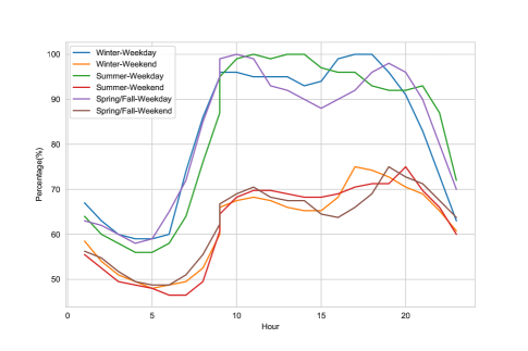
Figure 5: The expected electricity demand in percent of annual peak load.

The renewable energy resources of both solar and wind are considered in our experiments and the intermittency of solar/wind plants’ outputs are modeled. The solar intensity varies among different seasons, yielding various power generations. Figure 6 Left shows the hour-to-hour expected power output compared to the generating capacity of a solar plant within a day for each season. We assume that the energy generated by a solar farm in each hour follows a normal distribution and the standard deviation is 10% of its mean. The variability of wind speed also propagates to the power output of wind generators. Weibull distribution is a good fit to the probability distribution of wind speed in a region (Sansavini et al. 2014). As shown in Figure 6 Right, we consider a Weibull distribution with distinct scale and shape parameters for each season. In our experiments, we assume that a wind generator starts producing power when wind speed equals the cutin speed of $3m/s$, and the power out grows linearly with the wind speed until it reaches the maximum (i.e., the generating capacity of the generator) at the speed of $12m/s$.

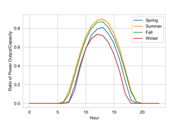
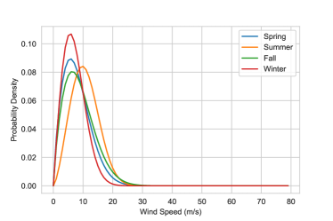
Figure 6: Left: The expected ratio of power output to generating capacity of a solar farm within a day in different seasons; Right: Weibull distributions of wind speed values in different seasons.

Appendix C Appendix to 6-Bus System Data

The tested 6-Bus system includes two generators, four transmission lines, and three loads at the beginning of the planning horizon. There are $4$ candidate generators that can be built to expand the current power system, including 2 fossil fuel generators, 1 solar farm and 1 wind generator. In addition, three more transmission lines can be constructed to connect the sites, and two energy storage devices can be installed along with renewable energy power plants.

Table 8: Generators in the IEEE 6-Bus system

Unit	Bus No.	Existing	Generation Cost Coefficient			Startup Cost	Pmin	Pmax	Min On	Min Off	Ramp
		(Y/N)	a($)	b($/MW)	c($/MW2)	($)	(MW)	(MW)	(h)	(h)	(MW/h)
G1	1	Y	177	13.5	0.00045	100	100	220	4	4	50
G2	2	Y	130	40	0.001	200	10	100	2	3	40
Wind	6	N	0	0	0	0	0	50	0	0	50
G3	1	N	59	22.9	0.0098	45	10	50	1	1	25
G4	2	N	130	32.6	0.001	300	10	100	2	3	40
Solar	3	N	0	0	0	0	0	20	0	0	20

Table 9: Transmission lines in the IEEE 6-Bus system

Line No.	From Bus	To Bus	Existing (Y/N)	Flow Limit (MW)
L1	1	2	Y	200
L2	2	3	N	100
L3	1	4	Y	150
L4	2	4	Y	200
L5	4	5	N	200
L6	5	6	Y	200
L7	3	6	N	100

Table 10: Energy storage in the IEEE 6-Bus system

Storage No.	Bus No.	Existing (Y/N)	Capacity (MW)
S1	3	N	10
S2	6	N	10

Table 11: Load data in the IEEE 6-Bus system

Bus No.	Annual Peak Load (MW)
3	50
4	120
5	120

Appendix D Appendix to Modified IEEE 118-Bus System

The system is constructed according to the original data in (IIT 2003). It initially consists of 34 generators, 166 transmission lines and 91 loads. The total installed generating capacity is 4060 MW. The candidate facilities that can be built over the planning horizon include 20 generators (8 wind generators, 2 solar farms and 10 fossil fuel generators, with the total generating capacity of 3430 MW), 20 transmission lines and 10 energy storage devices.

Table 12: Generators in the modified IEEE 118-Bus system

Unit	Bus No.	Existing	Generation Cost			Starup Cost	Pmin	Pmax	Min On	Min Off	Ramp
		(Y/N)	a ($)	b ($/MWh)	c ($/MWh2̂)	($)	(MW)	(MW)	(h)	(h)	(MW/h)
G1	4	Y	31.67	26.2438	0.069663	40	5	30	1	1	15
G2	6	Y	31.67	26.2438	0.069663	40	5	30	1	1	15
G3	8	Y	31.67	26.2438	0.069663	40	5	30	1	1	15
WIND1	10	N	0	0	0	0	0	300	0	0	300
G4	12	Y	6.78	12.8875	0.010875	110	100	300	8	8	150
G5	15	Y	31.67	26.2438	0.069663	40	10	30	1	1	15
G6	18	Y	10.15	17.82	0.0128	50	25	100	5	5	50
G7	19	Y	31.67	26.2438	0.069663	40	5	30	1	1	15
WIND2	24	N	0	0	0	0	0	300	0	0	300
G8	25	Y	6.78	12.8875	0.010875	100	100	300	8	8	150
G9	26	N	32.96	10.76	0.003	100	100	350	8	8	175
G10	27	Y	31.67	26.2438	0.069663	40	8	30	1	1	15
G11	31	N	31.67	26.2438	0.069663	40	8	30	1	1	15
WIND3	32	N	0	0	0	0	0	100	5	5	100
G12	34	Y	31.67	26.2438	0.069663	40	8	30	1	1	15
G13	36	N	10.15	17.82	0.0128	50	25	100	5	5	50
G14	40	Y	31.67	26.2438	0.069663	40	8	30	1	1	15
G15	42	Y	31.67	26.2438	0.069663	40	8	30	1	1	15
WIND4	46	N	0	0	0	0	0	100	5	5	100
G16	49	Y	28	12.3299	0.002401	100	50	250	8	8	125
G17	54	N	28	12.3299	0.002401	100	50	250	8	8	125
G18	55	Y	10.15	17.82	0.0128	50	25	100	5	5	50
G19	56	N	10.15	17.82	0.0128	50	25	100	5	5	50
WIND5	59	N	0	0	0	0	0	200	8	8	200
G20	61	Y	39	13.29	0.0044	100	50	200	8	8	100
G21	62	N	10.15	17.82	0.0128	50	25	100	5	5	50
G22	65	Y	64.16	8.3391	0.01059	250	100	420	10	10	210
G23	66	N	64.16	8.3391	0.01059	250	100	420	10	10	210
WIND6	69	N	0	0	0	0	0	300	0	0	300
G24	70	Y	74.33	15.4708	0.045923	45	30	80	4	4	40
G25	72	N	31.67	26.2438	0.069663	40	10	30	1	1	15
G26	73	Y	31.67	26.2438	0.069663	40	5	30	1	1	15
G27	74	Y	17.95	37.6968	0.028302	30	5	20	1	1	10
G28	76	Y	10.15	17.82	0.0128	50	25	100	5	5	50
WIND7	77	Y	0	0	0	0	0	100	5	5	100
G29	80	Y	6.78	12.8875	0.010875	440	150	300	8	8	150
G30	82	N	10.15	17.82	0.0128	50	25	100	5	5	50
G31	85	Y	31.67	26.2438	0.069663	40	10	30	1	1	15
G32	87	Y	32.96	10.76	0.003	440	100	300	8	8	150
G33	89	Y	6.78	12.8875	0.010875	400	50	200	8	8	100
G34	90	Y	17.95	37.6968	0.028302	30	8	20	1	1	10
WIND8	91	Y	0	0	0	0	0	50	1	1	50
G35	92	Y	6.78	12.8875	0.010875	100	100	300	8	8	150
G36	99	N	6.78	12.8875	0.010875	100	100	300	8	8	150
G37	100	Y	6.78	12.8875	0.010875	110	100	300	8	8	150
G38	103	Y	17.95	37.6968	0.028302	30	8	20	1	1	10
G39	104	N	10.15	17.82	0.0128	50	25	100	5	5	50
SOLAR1	105	N	0	0	0	0	0	100	0	0	100
G40	107	Y	17.95	37.6968	0.028302	30	8	20	1	1	10
G41	110	N	58.81	22.9423	0.009774	45	25	50	2	2	25
G42	111	Y	10.15	17.82	0.0128	50	25	100	5	5	50
SOLAR2	112	N	0	0	0	0	0	100	0	0	100
G43	113	Y	10.15	17.82	0.0128	50	25	100	5	5	50
G44	116	Y	58.81	22.9423	0.009774	45	25	50	2	2	25

Table 13: Transmission lines in the modified IEEE 118-Bus system

From Bus	To Bus	Existing (Y/N)	Flow Limit (MW)	From Bus	To Bus	Existing (Y/N)	Flow Limit (MW)
1	2	Y	175	63	64	Y	500
1	3	Y	175	64	61	Y	500
4	5	Y	500	38	65	Y	500
3	5	Y	175	64	65	Y	500
5	6	Y	175	49	66	Y	500
6	7	Y	175	49	66	N	500
8	9	Y	500	62	66	Y	175
8	5	Y	500	62	67	Y	175
9	10	N	500	65	66	Y	500
4	11	Y	175	66	67	Y	175
5	11	Y	175	65	68	Y	500
11	12	Y	175	47	69	Y	175
2	12	Y	175	49	69	Y	175
3	12	Y	175	68	69	Y	500
7	12	Y	175	69	70	N	500
11	13	Y	175	24	70	Y	175
12	14	Y	175	70	71	Y	175
13	15	N	175	24	72	Y	175
14	15	Y	175	71	72	Y	175
12	16	Y	175	71	73	Y	175
15	17	Y	500	70	74	Y	175
16	17	Y	175	70	75	Y	175
17	18	Y	175	69	75	Y	500
18	19	Y	175	74	75	N	175
19	20	Y	175	76	77	Y	175
15	19	Y	175	69	77	Y	175
20	21	N	175	75	77	Y	175
21	22	Y	175	77	78	Y	175
22	23	Y	175	78	79	Y	175
23	24	Y	175	77	80	Y	500
23	25	Y	500	77	80	Y	500
26	25	Y	500	79	80	Y	175
25	27	Y	500	68	81	N	500
27	28	Y	175	81	80	Y	500
28	29	Y	175	77	82	Y	200
30	17	N	500	82	83	Y	200
8	30	Y	175	83	84	Y	175
26	30	Y	500	83	85	Y	175
17	31	Y	175	84	85	Y	175
29	31	Y	175	85	86	Y	500
23	32	Y	140	86	87	Y	500
31	32	Y	175	85	88	N	175
27	32	Y	175	85	89	Y	175
15	33	Y	175	88	89	Y	500
19	34	N	175	89	90	Y	500
35	36	Y	175	89	90	Y	500
35	37	Y	175	90	91	Y	175
33	37	Y	175	89	92	Y	500
34	36	Y	175	89	92	Y	500
34	37	Y	500	91	92	Y	175
38	37	Y	500	92	93	N	175
37	39	Y	175	92	94	Y	175
37	40	Y	175	93	94	Y	175
30	38	N	175	94	95	Y	175
39	40	Y	175	80	96	Y	175
40	41	Y	175	82	96	Y	175
40	42	Y	175	94	96	Y	175
41	42	Y	175	80	97	Y	175
43	44	Y	175	80	98	Y	175
34	43	Y	175	80	99	N	200
44	45	Y	175	92	100	Y	175
45	46	Y	175	94	100	Y	175
46	47	N	175	95	96	Y	175
46	48	Y	175	96	97	Y	175
47	49	Y	175	98	100	Y	175
42	49	Y	175	99	100	Y	175
42	49	Y	175	100	101	Y	175
45	49	Y	175	92	102	Y	175
48	49	Y	175	101	102	N	175
49	50	Y	175	100	103	Y	500
49	51	Y	175	100	104	Y	175
51	52	N	175	103	104	Y	175
52	53	Y	175	103	105	Y	175
53	54	Y	175	100	106	Y	175
49	54	Y	175	104	105	Y	175
49	54	Y	175	105	106	Y	175
54	55	Y	175	105	107	Y	175
54	56	Y	175	105	108	N	175
55	56	Y	175	106	107	Y	175
56	57	Y	175	108	109	Y	175
50	57	N	175	103	110	Y	175
56	58	Y	175	109	110	Y	175
51	58	Y	175	110	111	Y	175
54	59	Y	175	110	112	Y	175
56	59	Y	175	17	113	Y	175
56	59	Y	175	32	113	Y	500
55	59	Y	175	32	114	N	175
59	60	Y	175	27	115	Y	175
59	61	Y	175	114	115	Y	175
60	61	N	500	68	116	Y	500
60	62	Y	175	12	117	Y	175
61	62	Y	175	75	118	Y	175
63	59	Y	500	76	118	Y	175

Table 14: Energy storage in the IEEE 118-Bus system

Storage No.	Bus No.	Existing (Y/N)	Capacity (MW)
S1	10	N	20
S2	24	N	20
S3	32	N	20
S4	46	N	20
S5	59	N	20
S6	69	N	20
S7	77	N	20
S8	91	N	20
S9	105	N	20
S10	112	N	20

References

- Ahmed et al. (2003) Ahmed S, King AJ, Parija G (2003) A multi-stage stochastic integer programming approach for capacity expansion under uncertainty. Journal of Global Optimization 26:3–24.
- Barnhart et al. (1998) Barnhart C, Johnson EL, Nemhauser GL, Savelsbergh MWP, Vance PH (1998) Branch-and-price: Column generation for solving huge integer programs. Operations Research 46(3):316–329.
- Bean et al. (1992) Bean JC, Higle JL, Smith RL (1992) Capacity expansion under stochastic demands. Operations Research 40(Supplement 2):S210–S216.
- Birge and Louveaux (2011) Birge JR, Louveaux F (2011) Introduction to Stochastic Programming (New York: Springer), 2nd edition.
- California-ISO (2010) California-ISO (2010) 72-hour residual unit commitment (RUC). http://www.caiso.com/27ae/27aebe3060d40.html.
- Chen et al. (2018) Chen X, Lv J, McElroy MB, Han X, Nielsen CP, Wen J (2018) Power system capacity expansion under higher penetration of renewables considering flexibility constraints and low carbon policies. IEEE Transactions on Power Systems 33(6):6240–6253.
- Conejo et al. (2021) Conejo AJ, Hall NG, Long DZ, Zhang R (2021) Robust capacity planning for project management. INFORMS Journal on Computing URL http://dx.doi.org/10.1287/ijoc.2020.1033.
- Dantzig and Wolfe (1960) Dantzig GB, Wolfe P (1960) Decomposition principle for linear programs. Operations Research 8(1):101–111.
- Davis et al. (1987) Davis MHA, Dempster MAH, Sethi SP, Vermes D (1987) Optimal capacity expansion under uncertainty. Advances in Applied Probability 19(1):156–176.
- Defourny et al. (2012) Defourny B, Ernst D, Wehenkel L (2012) Multistage stochastic programming: A scenario tree based approach to planning under uncertainty. Sucar LE, Morales EF, Hoey J, eds., Decision theory models for applications in artificial intelligence: concepts and solutions, 97–143 (IGI Global).
- Dvorkin et al. (2017) Dvorkin Y, Fernández-Blanco R, Kirschen DS, Pandžić H, Watson J, Silva-Monroy CA (2017) Ensuring profitability of energy storage. IEEE Transactions on Power Systems 32(1):611–623.
- Eppen et al. (1989) Eppen GD, Martin RK, Schrage L (1989) A scenario approach to capacity planning. Operations Research 37(4):517–527.
- Gorman et al. (2019) Gorman W, Mills A, Wiser R (2019) Improving estimates of transmission capital costs for utility-scale wind and solar projects to inform renewable energy policy. Energy Policy 135:110994.
- Heitsch and Römisch (2009) Heitsch H, Römisch W (2009) Scenario tree modeling for multistage stochastic programs. Mathematical Programming 118(2):371–406.
- Herman and Ganz (1994) Herman O, Ganz Z (1994) The capacity expansion problem in the service industry. Computers & Operations Research 21:557–572.
- Hobbs et al. (2001) Hobbs BF, Rothkopf MH, O’Neil RP, Chao H (2001) The Next Generation of Electric Power Unit Commitment Models (Norwell, MA, USA: Kluwer Academic Publishers).
- Huang and Zheng (2020) Huang Z, Zheng QP (2020) A multistage stochastic programming approach for preventive maintenance scheduling of gencos with natural gas contract. European Journal of Operational Research 287(3):1036–1051, ISSN 0377-2217.
- IIT (2003) IIT (2003) Index of data illinois institute of technology. http://motor.ece.iit.edu/data/.
- Jena et al. (2017) Jena SD, Cordeau JF, Gendron B (2017) Lagrangian heuristics for large-scale dynamic facility location with generalized modular capacities. INFORMS Journal on Computing 29(3):388–404.
- Krishnan et al. (2016) Krishnan V, Ho J, Hobbs BF, Liu AL, McCalley JD, Shahidehpour M, Zheng QP (2016) Co-optimization of electricity transmission and generation resources for planning and policy analysis: review of concepts and modeling approaches. Energy Systems 7(2):297–332.
- Laguna (1998) Laguna M (1998) Applying robust optimization to capacity expansion of one location in telecommunications with demand uncertainty. Management Science 44(11-part-2):S101–S110.
- Laporte and Louveaux (1993) Laporte G, Louveaux FV (1993) The integer L-shaped methods for stochastic integer programs with complete recourse. Operations Research Letters 13:133–142.
- Lara et al. (2018) Lara CL, Mallapragada DS, Papageorgiou DJ, Venkatesh A, Grossmann IE (2018) Deterministic electric power infrastructure planning: Mixed-integer programming model and nested decomposition algorithm. European Journal of Operational Research 271(3):1037 – 1054.
- Li and Tirupati (1994) Li S, Tirupati D (1994) Dynamic capacity expansion problem with multiple products: Technology selection and timing of capacity additions. Operations Research 42(5):958–976.
- Liu et al. (2018) Liu Y, Sioshansi R, Conejo AJ (2018) Multistage stochastic investment planning with multiscale representation of uncertainties and decisions. IEEE Transactions on Power Systems 33(1):781–791.
- Luss (1982) Luss H (1982) Operations research and capacity expansion problems: A survey. Operations Research 30(5).
- Mejía-Giraldo and McCalley (2014) Mejía-Giraldo D, McCalley JD (2014) Maximizing future flexibility in electric generation portfolios. IEEE Transactions on Power Systems 29(1):279–288.
- Munoz and Mills (2015) Munoz FD, Mills AD (2015) Endogenous assessment of the capacity value of solar pv in generation investment planning studies. IEEE Transactions on Sustainable Energy 6(4):1574–1585.
- Munoz and Watson (2015) Munoz FD, Watson JP (2015) A scalable solution framework for stochastic transmission and generation planning problems. Computational Management Science 12(4):491–518.
- Padberg (1974) Padberg MW (1974) Perfect zero–one matrices. Mathematical Programming 6(1):180–196.
- Pineda and Morales (2018) Pineda S, Morales JM (2018) Chronological time-period clustering for optimal capacity expansion planning with storage. IEEE Transactions on Power Systems 33(6):7162–7170.
- Poncelet et al. (2016) Poncelet K, Delarue E, Six D, Duerinck J, D’haeseleer W (2016) Impact of the level of temporal and operational detail in energy-system planning models. Applied Energy 162:631–643.
- Powell et al. (2012) Powell WB, George A, Simao H, Scott W, Lamont A, Stewart J (2012) SMART: a stochastic multiscale model for the analysis of energy resources, technology, and policy. INFORMS Journal on Computing 24(4):665–682.
- Rajagopalan et al. (1998) Rajagopalan S, Singh MR, Morton TE (1998) Capacity expansion and replacement in growing markets with uncertain technological breakthroughs. Management Science 44:12–30.
- Riis and Andersen (2002) Riis M, Andersen KA (2002) Capacitated network design with uncertain demand. INFORMS Journal on Computing 14(3):247–260.
- Ryan and Falkner (1988) Ryan D, Falkner J (1988) On the integer properties of scheduling set partitioning models. European Journal of Operational Research 35(3):442 – 456.
- Sahinidis and Grossmann (1992) Sahinidis NV, Grossmann IE (1992) Reformulation of the multiperiod milp model for capacity expansion of chemical processes. Operations Research 40(1-supplement-1):S127–S144.
- Sansavini et al. (2014) Sansavini G, Piccinelli R, Golea L, Zio E (2014) A stochastic framework for uncertainty analysis in electric power transmission systems with wind generation. Renewable Energy 64:71 – 81.
- Santoso et al. (2005) Santoso T, Ahmed S, Goetschalckx M, Shapiro A (2005) A stochastic programming approach for supply chain network design under uncertainty. European Journal of Operational Research 167(1):96 – 115.
- Schoenung (2011) Schoenung SM (2011) Energy storage systems cost update : a study for the doe energy storage systems program. URL http://dx.doi.org/10.2172/1013227.
- Sen et al. (2006) Sen S, Yu L, Genc T (2006) A stochastic programming approach to power portfolio optimization. Operations Research 54:55–72.
- Shiina and Birge (2003) Shiina T, Birge J (2003) Multistage stochastic programming model for electric power capacity expansion problem. Japan Journal of Industrial and Applied Mathematics 20:379–397.
- Singh et al. (2009) Singh KJ, Philpott AB, Wood KR (2009) Dantzig-Wolfe decomposition for solving multistage stochastic capacity-planning problems. Operations Research 57:1271–1286.
- Teichgraeber and Brandt (2019) Teichgraeber H, Brandt AR (2019) Clustering methods to find representative periods for the optimization of energy systems: An initial framework and comparison. Applied Energy 239:1283–1293, ISSN 0306-2619.
- US-EIA (2019) US-EIA (2019) Annual energy outlook 2019. https://www.eia.gov/outlooks/aeo/.
- US-EIA (2020) US-EIA (2020) Capital cost and performance characteristic estimates for utility scale electric power generating technologies. https://www.eia.gov/analysis/studies/powerplants/capitalcost/pdf/capital_cost_AEO2020.pdf.
- Wallace and Fleten (2003) Wallace SW, Fleten SE (2003) Stochastic programming models in energy. Ruszczynski A, Shapiro A, eds., Stochastic Programming, volume 10, 637–677 (Elsevier).
- Wu et al. (2016) Wu Z, Zeng P, Zhang X, Zhou Q (2016) A solution to the chance-constrained two-stage stochastic program for unit commitment with wind energy integration. IEEE Transactions on Power Systems 31(6):4185–4196.
- Xiao et al. (2011) Xiao J, Hodge BS, Liu AL, Pekny JF, Reklaitis GV (2011) Long-term planning of wind farm siting in the electricity grid. Proceeds of the 21st European Symposium on Computer Aided Process Engineering-ESCAPE 21.
- Zheng et al. (2013) Zheng QP, Wang J, Pardalos PM, Guan Y (2013) A decomposition approach to the two-stage stochastic unit commitment problem. Annals of Operations Research 210(1):387–410.
- Zolfaghari Moghaddam (2019) Zolfaghari Moghaddam S (2019) Generation and transmission expansion planning with high penetration of wind farms considering spatial distribution of wind speed. International Journal of Electrical Power & Energy Systems 106:232–241.
- Zou et al. (2018) Zou J, Ahmed S, Sun XA (2018) Partially adaptive stochastic optimization for electric power generation expansion planning. INFORMS Journal on Computing 30(2):388–401.