An Information Theory-inspired Strategy for Automatic Network Pruning

Abstract

Despite superior performance on many computer vision tasks, deep convolution neural networks are well known to be compressed on devices that have resource constraints. Most existing network pruning methods require laborious human efforts and prohibitive computation resources, especially when the constraints are changed. This practically limits the application of model compression when the model needs to be deployed on a wide range of devices. Besides, existing methods are still challenged by the missing theoretical guidance. In this paper we propose an information theory-inspired strategy for automatic model compression. The principle behind our method is the information bottleneck theory, i.e., the hidden representation should compress information with each other. We thus introduce the normalized Hilbert-Schmidt Independence Criterion (nHSIC) on network activations as a stable and generalized indicator of layer importance. When a certain resource constraint is given, we integrate the HSIC indicator with the constraint to transform the architecture search problem into a linear programming problem with quadratic constraints. Such a problem is easily solved by a convex optimization method with a few seconds. We also provide a rigorous proof to reveal that optimizing the normalized HSIC simultaneously minimizes the mutual information between different layers. Without any search process, our method achieves better compression trade-offs comparing to the state-of-the-art compression algorithms. For instance, with ResNet-$50$, we achieve a $45.3\%$-FLOPs reduction, with a $75.75$ top-1 accuracy on ImageNet. Codes are avaliable at https://github.com/MAC-AutoML/ITPruner.

1 Introduction

While convolutional neural networks (CNNs) [23] have demonstrated great success in various computer vision tasks, such as classification [13, 22], detection [39, 10] and semantic segmentation [5, 32]. However, their large demands of computation power and memory footprint make most state-of-the-art CNNs notoriously challenging to deploy on resource-limited devices such as smartphones or wearable devices. Lots of research resources have been devoted to CNN compression and acceleration, including but not limited to parameter quantization [19, 53], filter compression [50, 34, 25] and automatic network pruning [51, 48, 8, 30, 52, 14].

Among these compression methods, automatic network pruning has recently attracted a lot of attentions and has been successfully applied to state-of-the-art architectures, such as EfficientNet [46], MnasNet [45] and MobileNetV3 [16]. Given a pre-trained network, the compression method aims to automatically simplify the channel of the network until the resource budget is met while maximizing the accuracy. It is also named as channel number search [8, 52, 48], automatic model compression [14] or network adaption [51]. Based on the design of the methodology, we empirically categorize network pruning methods into two groups and discuss them as below.

Metric based methods compress the size of a network by selecting filters rely on hand-crafted metrics. We can further divide existing metrics into two types, local metrics [25, 34, 50] and global metrics [28, 36]. The first pursues to identify the importance of filters inside a layer. In other words, local metric based methods require human experts to design and decide hyper-parameters like channel number and then pruning filters in each layer according to $L1$ norm [25] or geometric median [15]. These methods are not automatic and thus less practical in compressing various models. In addition, extensive experiments in [4, 31] suggest that filter-level pruning does not help as much as selecting a better channel number for a specific architecture. The second designs a metric to compare the importance of filters across different layers. Such methods implicitly decide the channel number and thus alleviate the large amount of human efforts compared to local metric based methods. However, these methods usually perform network pruning followed by a data-driven and/or iterative optimization to recover accuracy, both of which are time-cost.

Search based methods. Apart from these human-designed heuristics, efforts on search based methods have been made recently. The main difference between these methods lies in the search algorithm and architecture evaluation method. In term of search algorithm, AMC [14] and NetAdapt [51] leverage reinforcement learning to efficiently sample the search space. Autoslim [52] greedily slim the layer with minimal accuracy drop. In terms of the evaluation method, existing methods usually adopt weight sharing strategy to evaluate the accuracy [48, 8, 30, 52, 14]. To explain, weight sharing methods maintain an over-parameterized network that covers the entire search space. The sampled architectures directly inherit the corresponding weights from the over-parameterized network, which is then used to evaluate the performance and update the weights. Both of these methods require recompression or retraining while the constraints changing. This practically limits the application of network pruning since the model needs to be deployed on a wide range of devices.

In this paper, we propose an information theory-inspired pruning (ITPruner) strategy that does not need the aforementioned iterative training and search process, which is simple and straightforward. Specifically, we first introduce the normalized Hilbert-Schmidt Independence Criterion (nHSIC) on network activations as an accurate and robust layer-wise importance indicator. Such importance is then combined with the constraint to convert the architecture search problem to a linear programming problem with bounded variables. In this way, we obtain the optimal architecture by solving the linear programming problem, which only takes a few seconds on a single CPU and GPU.

Our method is motivated by the information bottleneck (IB) theory [47]. That is, for each network layer we should minimize the information between the layer activation and input. We generalize such a principle to different layers for automatic network pruning, i.e., a layer correlated to other layers is less important. In other words, we build a connection between network redundancy and information theory. However, calculating the mutual information among the intractable distribution of the layer activation is impractical. We thus adopt a non-parametric kernel-based method the Hilbert-Schmidt Independence Criterion (HSIC) to characterize the statistical independence. In summary, our contributions are as follows:

• Information theory on deep learning redundancy. To our best knowledge, this is the first to build a relationship between independence and redundancy of CNN by generalizing the information bottleneck principle. We are also the first that apply such relationship in automatic network pruning.

• Methodology. We propose a unified framework to automatically compress a network without any search process. The framework integrates HSIC importance with constraints to transform the network pruning to the convex optimization problem, which is efficient of the deployment on various devices.

• Theoretical contributions. Except for the potential theoretical guarantees of HSIC, we also theoretically prove the robustness of HSIC as well as the relationship between our method and mutual information. In particular, as proved in Sec. 4, optimizing HSIC is equivalent to minimize the layer-wise mutual information under the gaussian modeling.

The experimental results demonstrate the efficiency and effectiveness on different network architectures and datasets. Notably, without any search process, our compressed MobileNetV1 obtain $50.3\%$ FLOPs reduction with $70.92$ Top-1 accuracy. Meanwhile, the compressed MobileNet V2, ResNet-50 and MobileNet V1 obtained by ITPruner achieve the best performance gains over the state-of-the-art AutoML methods.

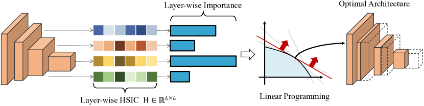
Figure 1: Overview of our ITpruner. Specifically, We first samples $n$ images to obtain the feature map of each layer. Then the normalized HSIC is employed to calculate the independence map $\boldsymbol{H}$ between different layers. For each layer, we sum the elements of the corresponding column in $\boldsymbol{H}$ except for itself as the importance indicator of the layer. In this way, we model the layer-wise importance and compression constraints as a linear programming problem. Finally, the optimal network architecture is obtained by solving the optimal solution on the linear programming.

2 Related Work

There are a large amount works that aim at compressing CNNs and employing information theory into deep learning, where the main approaches are summarized as follows.

Automatic Network Pruning. Following previous works [51, 48, 8, 30, 52, 14], automatic network pruning adapts channels of a pre-trained model automatically to a specific platform (e.g., mobile, IoT devices) under a given resource budget. Similar works that modifying channels to reduce its FLOPs and speedup its inference have been proposed [50, 34, 25, 48, 8, 30, 52, 14] in the literature, which is known as network pruning. Most of the pruning-based methods have been discussed in Sec. 1. Therefore, we select the two most related works [36, 28], which proposed to prune networks by designing a global metric. However, these methods are still far from satisfactory. On one hand, there is a significant performance and architecture gap compared to search based methods [30, 52, 14]. On the other hand, these methods also need an extra iterative optimization step to recover the performance. In this case, search based methods and global metric based methods require almost the same computation resources. In contrast, our method shows superior performance compared to search based methods. Besides, we do not need any iterative training or search in our method and generating an optimal architecture only takes a few seconds.

Information theory[6] is a fundamental research area which often measures information of random variables associated with distributions. Therefore, a lot of principles and theories have been employed to explore the learning dynamic [11, 2] or as a training objective to optimize the network without stochastic gradient descent [35, 43]. To our best knowledge, there exist only two prior works [7, 1] that apply information theory in network compression. Dai et al. proposed to compress the network using variation information bottleneck [47]. However, their metric measures importance inside a specific layer, which is not automatic and less effective. Ahn et al. proposed a variational information distillation method, aiming to distill the knowledge from teacher to the student. Such a method is orthogonal to our method. In other words, we can employ the method as a post-processing step to further improve the performance.

3 Methodology

Notations. Upper case (e.g.,$X,Y$) denotes random variables. Bold denotes vectors (e.g.,$\boldsymbol{x,y}$), matrices (e.g.,$\boldsymbol{X,Y}$) or tensors. Calligraphic font denotes spaces (e.g.,$\mathcal{X},\mathcal{Y}$). We further define some common notations in CNNs. The $l$-th convolutional layer in a specific CNN convert an input tensor $\boldsymbol{X}^{l}\in\mathbb{R}^{c^{l}\times h_{\text{in}}^{l}\times w_{\text{in}}^{l}}$ to an output tensor $\boldsymbol{Y}^{l}\in\mathbb{R}^{n^{l}\times h_{\text{out}}^{l}\times w_{\text{out}}^{l}}$ by using a weight tensor $\boldsymbol{W}^{l}\in\mathbb{R}^{n^{l}\times c^{l}\times k^{l}\times k^{l}}$, where $c^{l}$ and $n^{l}$ denote the numbers of input channels and filters (output channels), respectively, and $k^{l}\times k^{l}$ is the spatial size of the filters.

Problem formulation. Given a pre-trained CNN model that contains $L$ convolutional layers, we refer to $\boldsymbol{\alpha}=(\alpha_{1},\alpha_{2},...,\alpha_{L})$ as the desired architecture, where $\alpha_{l}$ is the compression ratio of $l$-th layers. Formally, we address the following optimization problem:

$$\max_{\boldsymbol{W}\in\mathcal{W},\boldsymbol{\alpha}\in\mathcal{A}}f(\boldsymbol{W},\boldsymbol{\alpha}),\,s.t.\;T(\boldsymbol{\alpha})<{\Omega},$$ (1)

where $f:\mathcal{W}\times\mathcal{A}\rightarrow\mathbb{R}$ is the objective function that is differentiable w.r.t. the network weight $\boldsymbol{W}\in\mathcal{W}$, and is not differentiable w.r.t. the architecture indicator vector $\boldsymbol{\alpha}\in\mathcal{A}\in\mathbb{R}^{L\times 1}$. $T(.)$ is a function that denotes the constraints for architectures, such as FLOPs and latency, and $\Omega$ is given for different hardwares.

We present an overview of ITPruner in Fig. 1, which aims to automatically discover the redundancy of each layer in a pre-trained network. Notably, the redundancy is also characterized by the layer-wise pruning ratio or sparsity. The detailed motivations, descriptions and analysis are presented in the following sub-sections.

3.1 Information Bottleneck in Deep Learning

The information bottleneck (IB) [47] principle express a tradeoff of mutual information from the hidden representation to input and output, which is formally defined as

$$\min_{p(X_{i}|X)}I(X;X_{i})-\beta I(X_{i};Y),$$ (2)

where $X,Y$ are the random variables of input and label, and $X_{i}$ represents the hidden representation. Intuitively, the IB principle is proposed to compress the mutual information between the input and the hidden representation while preserving the information between the hidden representation about the input data. Considering that CNNs are hierarchical and almost all of CNNs are adopted from residual neural networks, we further generalize the IB principle in Eq. 2 as

$$\min_{p(X_{i}|X)}\sum_{i=1}^{L}\sum_{j=i+1}^{L}\left(I(X;X_{i})+I(X_{j};X_{i})\right)-\beta I(X_{i};Y).$$ (3)

Note that there always a fine-tuning process in the pruning process. We thus further simplify the IB principle as

$$\min_{p(X_{i}|X)}\sum_{i=1}^{L}\sum_{j=i+1}^{L}\left(I(X;X_{i})+I(X_{j};X_{i})\right).$$ (4)

According to the generalized IB principle, we hope that the mutual information between different layers is close to $0$. In other words, representations from different layers are best to be independent of each other. We thus generalize such a principle in network compression, i.e., a layer correlated to other layers is less important. Meanwhile, layer-wise mutual information can be considered as a robust and accurate indicator to achieve search-free automatic network pruning.

The IB is hard to compute in practice. On one hand, the distribution of the hidden representation is intractable in CNN. Previous work [1] define a variational distribution that approximates the distribution. However, such a method also introduces a new noise between the approximated and true distribution, which is inevitable as the Kullback-Leiber divergence is non-negative. On the other hand, the hidden representations usually have a high dimension in CNN. In this case, many algorithms based on binning suffers from the curse of dimensionality. Besides, they also yield different results with different bin sizes.

3.2 Normalized HSIC Indicator

To solve the issues in Sec. 3.1, we introduce the normalized HSIC to replace the mutual information term in Eq. 4. Formally, the Hilbert-Schmidt Independence Criterion (HSIC) [12] is defined as

$$\text{HSIC}( P_{XY},\mathcal{H},\mathcal{G})=||C_{XY}||^{2}$$ (5)

$$=\mathbb{E}_{X,X^{{}^{\prime}},Y,Y^{{}^{\prime}}}[k_{X}(X,X^{{}^{\prime}})k_{Y}(Y,Y^{{}^{\prime}})]$$

$$+\mathbb{E}_{X,X^{{}^{\prime}}}[k_{X}(X,X^{{}^{\prime}})]\mathbb{E}_{Y,Y^{{}^{\prime}}}[k_{Y}(Y,Y^{{}^{\prime}})]$$

$$-2\mathbb{E}_{XY}[\mathbb{E}_{X^{{}^{\prime}}}[k_{X}(X,X^{{}^{\prime}})]\mathbb{E}_{Y^{{}^{\prime}}}[k_{Y}(Y,Y^{{}^{\prime}})]].$$

Here $k_{X},k_{Y}$ are kernel functions, $\mathcal{H},\mathcal{G}$ are the Reproducing Kernel Hilbert Space (RKHS) and $\mathbb{E}_{X,X^{{}^{\prime}},Y,Y^{{}^{\prime}}}$ denotes the expectation over independent examples $(x,y),(x^{{}^{\prime}},y^{{}^{\prime}})$ drawn from $p_{xy}$. In order to make HSIC practically available, Gretton et al. [12] further proposed to empirically approximate $\text{HSIC}(P_{XY},\mathcal{H},\mathcal{G})$ given a finite number of observations. Specifically, let $\mathcal{D}:=\{(x_{1},y_{1}),...,(x_{n},y_{n})\}$ contain $n$ i.i.d samples drawn from the distribution $P_{XY}$. The estimation of HSIC is given by

$$\text{HSIC}(\mathcal{D},\mathcal{F},\mathcal{G})=(n-1)^{-2}\text{tr}(\boldsymbol{K}_{X}\boldsymbol{H}\boldsymbol{K}_{Y}\boldsymbol{H}),$$ (6)

where $\boldsymbol{K}_{X},\boldsymbol{K}_{Y},\boldsymbol{H}\in\mathbb{R}^{n\times n}$, $\boldsymbol{K}_{X}$ and $\boldsymbol{K}_{Y}$ have entries $\boldsymbol{K}_{X(i,j)}=k(x_{i},x_{j})$, and $\boldsymbol{H}=\boldsymbol{I}_{n}-\frac{1}{n}\boldsymbol{1}_{n}\boldsymbol{1}^{T}_{n}$ is the centering matrix. Notably, an alternative implementation of $\boldsymbol{H}$ is to centralize the examples, i.e., $x_{i}=x_{i}-\mu_{X}$, where $\mu_{X}=\frac{1}{n}\sum_{i}X_{i}$. In this way, Eq. 6 is further simplified as

$$\text{HSIC}(X,Y)=(n-1)^{-2}\text{tr}(\boldsymbol{K}_{X}\boldsymbol{K}_{Y}),$$ (7)

where $\boldsymbol{K}_{X},\boldsymbol{K}_{Y}$ are centralized matrices. In our paper, we use the normalized HSIC (nHSIC) based on the centered kernel alignment [20], given by

$$\text{nHSIC}(X,Y)=\frac{\text{tr}(\boldsymbol{K}_{X}\boldsymbol{K}_{Y})}{\sqrt{\text{tr}(\boldsymbol{K}_{X}\boldsymbol{K}_{X})}\sqrt{\text{tr}(\boldsymbol{K}_{Y}\boldsymbol{K}_{Y})}}$$ (8)

The HSIC can be effectively computed in $\mathcal{O}(n^{2})$ time. Meanwhile, the uniform convergence bounds derived in [12] with respect to $P_{XY}$ is $\mathcal{O}(n^{-\frac{1}{2}})$. When an appropriate kernel is selected, $\text{HSIC}=0$ if and only if the random variables $X,Y$ are independent, i.e., $P_{XY}=P_{X}P_{Y}$. We also provide proof in Sec. 4 to demonstrate the relationship between HSIC and mutual information: When the linear kernel is selected, minimizing HSIC is equivalent to minimize the mutual information under a Gaussian assumption. Meanwhile, in this case, nHSIC is also equivalent to the RV coefficient [40] and Tucker’s congruence coefficient [33].

3.3 Pruning Strategy

We now describe how to use the nHSIC to compress a network under an optimal trade-off between compression rate and accuracy. Specifically, we first sample $n$ images to obtain the feature map of each layer $\boldsymbol{X}^{1},\boldsymbol{X}^{2},...,\boldsymbol{X}^{L}$ for the network that needs to be compressed. We then use these feature maps and Eq. 8 to get the independence between different layers, thereby constructing an independence matrix $\boldsymbol{H}\in\mathbb{R}^{L\times L}$, where $\boldsymbol{H}$ has entries $\boldsymbol{H}_{i,j}=\text{nHSIC}(\boldsymbol{X^{i}},\boldsymbol{X^{j}})$. As mentioned before, a layer correlated to other layers is less important. Therefore, the importance of a specific layer $l$ is formally defined as

$$\boldsymbol{i}^{l}=e^{-\beta\sum_{i=1,i\neq l}^{L}\text{nHSIC}(\boldsymbol{X}^{l},\boldsymbol{X}^{i})},$$ (9)

where $\beta$ is proposed to control relative compression rate between different layers. To explain, the compressed network tend to has a significant compression rate difference between different layers with a small $\beta$, and vice versa. We also provide extensive experiments in Sec. 5 to verify the conclusion. With the layer-wise importance $\boldsymbol{i}\in\mathbb{R}^{L\times 1}$, the problem of Eq. 1 is transformed to a linear programming problem that is differentiable w.r.t $\alpha$. Formally, Eq. 1 is rewritten as

$$\max_{\boldsymbol{\alpha}}\,\boldsymbol{i}^{T}\boldsymbol{\alpha}\,s.t.\;T(\boldsymbol{\alpha})<{\Omega}.$$ (10)

In most cases, the constraints such as FLOPs, parameters and inference time can be decomposed to the sum over different layers. Therefore, Eq. 10 is further simplified to a linear programming with quadratic constraints

$$\max_{\boldsymbol{\alpha}}\,\boldsymbol{i}^{T}\boldsymbol{\alpha}\,s.t.\;\boldsymbol{\alpha}^{T}\boldsymbol{T}\boldsymbol{\alpha}<{\Omega},$$ (11)

where $\boldsymbol{T}\in\mathbb{R}^{L\times L}$ is the constraint factor matrix corresponding to the layers. For example, suppose we choose the parameter size as the constraint. In this case, for a specific layer $l$, the parameter size of the layer is correlated to the input and the output channels, i.e., parameter size in $l$-th layer is $\alpha^{l}n^{l}\times\alpha^{l-1}c^{l}\times k^{l}\times k^{l}$. Therefore, the constraints are quadratic in Eq. 11. Note that solving the problem in Eq. 11 is extremely effective, which only takes a few seconds on a single CPU by using the solver in [21]. Our proposed ITPruner is also summarized in Alg. 1.

Input: Sampled $n$ i.i.d samples $\mathcal{D}$, pre-trained model $\mathcal{M}$.

Output: Optimized architecture $\boldsymbol{\alpha}^{*}$.

1 Input $\mathcal{D}$ into $\mathcal{M}$ to generate layer-wise feature map $\boldsymbol{X}^{1},...,\boldsymbol{X}^{L}$;

2 Obtain the independent matrix $\boldsymbol{H}$ by using Eq. 8;

3 Calculate the layer-wise importance $\boldsymbol{i}$ by Eq. 9;

$\alpha^{*}=\operatorname*{arg\,max}_{\boldsymbol{\alpha}}\,\boldsymbol{i}^{T}\boldsymbol{\alpha}\,s.t.\;\boldsymbol{\alpha}^{T}\boldsymbol{T}\boldsymbol{\alpha}<{\Omega}$ ;

Algorithm 1 ITPruner

Discussion. Compared to previous methods [48, 8, 30, 52, 14], ITPruner is effective and easy to use. In terms of effectiveness, our method does not need any training and search process to obtain the optimal architecture. The time complexity is only correlated to the sample number $n$, i.e., $\mathcal{O}(n)$ in the feature generation and $\mathcal{O}(n^{2})$ in HSIC calculation, both of them only take a few seconds on a single GPU and CPU, respectively. In terms of usability, there are only two hyper-parameters $n$ and $\beta$ in our method. Meanwhile, $n$ and $\beta$ are generalized to different architectures and datasets. Extensive experiments in Sec. 5.3 demonstrate that the performance gap between different $\beta$ and $n$ is negligible. This is in stark contrast to the previous search based methods, as they need to exhaustedly select a large amount of hyper-parameters for different architectures.

4 Theoretical Analysis

In this section, we provide theoretical analysis about the proposed method. Specifically, the invariance of scale and orthogonal transformation is already proposed in [20], which is also the key property of feature similarity metric [20] in deep learning. Here we provide the strict proofs about the aformentioned invariance in Theorem 1 and Theorem 2 respectively. To further explain the relationship between $\text{nHSIC}_{\text{linear}}$ and mutual information, we theoretically prove that optimizing $\text{nHSIC}_{\text{linear}}$ is equivalent to minimizing the mutual information in Theorem 3.

To make the implementation easy, we use linear kernel $k(\boldsymbol{x},\boldsymbol{y})=\boldsymbol{x}^{T}\boldsymbol{y}$ in all our experiments. In this case, $\boldsymbol{K}_{X}=XX^{T},\boldsymbol{K}_{Y}=YY^{T}$. And nHSIC is further simplified as

$$\text{nHSIC}_{\text{linear}}(X,Y)$$ (12)

$$=\frac{\text{tr}\left(\boldsymbol{XX}^{T}\boldsymbol{YY}^{T}\right)}{\sqrt{\text{tr}\left(\boldsymbol{XX}^{T}\boldsymbol{XX}^{T}\right)}\sqrt{\text{tr}\left(\boldsymbol{YY}^{T}\boldsymbol{YY}^{T}\right)}}$$

$$=\frac{\left\langle\text{vec}\left(\boldsymbol{XX}^{T}\right),\text{vec}\left(\boldsymbol{YY}^{T}\right)\right\rangle}{\sqrt{\left\langle\text{vec}\left(\boldsymbol{XX}^{T}\right),\text{vec}\left(\boldsymbol{XX}^{T}\right)\right\rangle}\sqrt{\left\langle\text{vec}\left(\boldsymbol{YY}^{T}\right),\text{vec}\left(\boldsymbol{YY}^{T}\right)\right\rangle}}$$

$$=\frac{||\boldsymbol{Y}^{T}\boldsymbol{X}||_{F}^{2}}{||\boldsymbol{X}^{T}\boldsymbol{X}||_{F}||\boldsymbol{Y}^{T}\boldsymbol{Y}||_{F}},$$

where $||.||_{F}$ is Frobenius norm or the Hilbert-Schmidt norm. Eq. 12 is easy to compute and has some useful properties of being invariant to scale and orthogonal transformations. To explain, we provide two formal theorems and the corresponding proofs as follows

Theorem 1.

$\text{nHSIC}_{\text{linear}}$ is invariant to scale transformation, i.e., $\text{nHSIC}_{\text{linear}}(\beta X,Y)=\text{nHSIC}_{\text{linear}}(X,Y)$.

Proof.

$$\text{nHSIC}_{\text{linear}}(\beta X,Y) =\frac{\beta^{2}||\boldsymbol{Y}^{T}\boldsymbol{X}||_{F}^{2}}{\beta\cdot||\boldsymbol{X}^{T}\boldsymbol{X}||_{F}\beta\cdot||\boldsymbol{Y}^{T}\boldsymbol{Y}||_{F}}$$

$$=\text{nHSIC}_{\text{linear}}(X,Y).$$

∎

Theorem 2.

$\text{nHSIC}_{\text{linear}}$ is invariant to orthogonal transformation $\text{nHSIC}_{\text{linear}}(X\boldsymbol{U},Y)=\text{nHSIC}_{\text{linear}}(X,Y)$, where $\boldsymbol{U}\boldsymbol{U}^{T}=\boldsymbol{I}$.

Proof.

$$\text{nHSIC}_{\text{linear}}(X\boldsymbol{U},Y)$$

$$=\frac{||\boldsymbol{Y}^{T}\boldsymbol{X}\boldsymbol{U}||_{F}^{2}}{||\boldsymbol{U}^{T}\boldsymbol{X}^{T}\boldsymbol{X}\boldsymbol{U}||_{F}||\boldsymbol{Y}^{T}\boldsymbol{Y}||_{F}}$$

$$=\frac{tr(\boldsymbol{X}\boldsymbol{U}\boldsymbol{U}^{T}\boldsymbol{X}^{T}\boldsymbol{Y}\boldsymbol{Y}^{T})}{\sqrt{tr(\boldsymbol{X}\boldsymbol{U}\boldsymbol{U}^{T}\boldsymbol{X}^{T}\boldsymbol{X}\boldsymbol{U}\boldsymbol{U}^{T}\boldsymbol{X}^{T})}||\boldsymbol{Y}^{T}\boldsymbol{Y}||_{F}}$$

$$=\frac{tr(\boldsymbol{X}\boldsymbol{X}^{T}\boldsymbol{Y}\boldsymbol{Y}^{T})}{\sqrt{tr(\boldsymbol{X}\boldsymbol{X}^{T}\boldsymbol{X}\boldsymbol{X}^{T})}||\boldsymbol{Y}^{T}\boldsymbol{Y}||_{F}}$$

$$=\frac{||\boldsymbol{Y}^{T}\boldsymbol{X}||_{F}^{2}}{||\boldsymbol{X}^{T}\boldsymbol{X}||_{F}||\boldsymbol{Y}^{T}\boldsymbol{Y}||_{F}}$$

$$=\text{nHSIC}_{\text{linear}}(X,Y),$$

which means that $\text{nHSIC}_{\text{linear}}$ is invariant to orthogonal transformation. ∎

Theorem 1 and 2 illustrate the robustness of $\text{nHSIC}_{\text{linear}}$ in different network architectures. Specifically, when the network architecture contain the batch normalization [18] or $1\times 1$ orthogonal convolution layer [49], we can obtain exactly the same layer-wise importance $\boldsymbol{i}$, and thus obtain a same network architecture. Considering that ITPruner has a superior performance in different architectures and datasets, we conclude that $\text{nHSIC}_{\text{linear}}$ is a stable and accurate indicator. And ITPruner thus is a robust compression method.

Except for the theorem about the relationship between independence and HSIC in [12], we propose a new theorem to illustrate how the mutual information is also minimized by the linear HSIC under a Gaussian assumption.

Theorem 3.

Assuming that $X\sim\mathcal{N}(\boldsymbol{0},\boldsymbol{\Sigma}_{X}),Y\sim\mathcal{N}(\boldsymbol{0},\boldsymbol{\Sigma}_{Y})$, $\min\text{nHSIC}_{\text{linear}}(X,Y)\iff\min I(X;Y)$.

Proof.

According to the definition of entropy and mutual information, we have

$$I(X;Y)=H(X)+H(Y)-H(X,Y).$$

Meanwhile, according to the definition of the multivariate Gaussian distribution, we have

$$H(X)=\frac{1}{2}\ln\left(\left(2\pi e\right)^{D}|\boldsymbol{\Sigma}_{X}|\right)=\frac{D}{2}(\ln 2\pi+1)+\frac{1}{2}\ln|\boldsymbol{\Sigma}_{X}|,$$

and $(X,Y)\sim\mathcal{N}(\boldsymbol{0},\boldsymbol{\Sigma}_{(X,Y)})$, where

$$\boldsymbol{\Sigma}_{(X,Y)}=\begin{pmatrix}\boldsymbol{\Sigma}_{X}&\boldsymbol{\Sigma}_{XY}\\ \boldsymbol{\Sigma}_{YX}&\boldsymbol{\Sigma}_{Y}\\ \end{pmatrix}.$$

Therefore, when $X,Y$ follows a Gaussian distribution, the mutual information is represented as

$$I(X;Y)=\ln|\boldsymbol{\Sigma}_{X}|+\ln|\boldsymbol{\Sigma}_{Y}|-\ln|\boldsymbol{\Sigma}_{(X,Y)}|.$$ (13)

Everitt et al. [9] proposed a inequation that $|\boldsymbol{\Sigma}_{(X,Y)}|\leq|\boldsymbol{\Sigma}_{X}||\boldsymbol{\Sigma}_{Y}|$, and the equality holds if and only if $\boldsymbol{\Sigma}_{YX}=\boldsymbol{\Sigma}_{XY}^{T}=\boldsymbol{X}^{T}\boldsymbol{Y}$ is a zero matrix. Applying the inequation to Eq. 13 we have $I(X;Y)\geq 0$, and the equality holds if and only if $\boldsymbol{X}^{T}\boldsymbol{Y}$ is a zero matrix. According to the defination of Frobenius norm, we have $||\boldsymbol{Y}^{T}\boldsymbol{X}||_{F}^{2}=||\boldsymbol{X}^{T}\boldsymbol{Y}||_{F}^{2}$. Apparently, when minimizing Eq. 12, we are also minimizing the distance between $\boldsymbol{X}^{T}\boldsymbol{Y}$ and zero matrix. In other words, while minimizing $\text{nHSIC}_{\text{linear}}$, we are also minimizing the mutual information between two Gaussian distributions, namely, $\min\text{nHSIC}_{\text{linear}}(X,Y)\iff\min I(X;Y).$ ∎

Model	Method	Type	Top-1 Acc	$\uparrow\downarrow$	FLOPs	Ratio$\downarrow$	Search
			($\%$)		(M)		Epoch
VGG [44]	Baseline	-	$94.47$	-	$313.5$	-	-
	L1 [25]	Local Metric	$93.4$	$1.07\downarrow$	$206$	$34.3\%$	-
	FPGM [15]	Local Metric	$93.54$	$0.93\downarrow$	$201.1$	$35.9\%$	-
	GAL [29]	Local Metric	$92.03$	$2.44\downarrow$	$189.5$	$39.6\%$	-
	HRank [26]	Local Metric	$92.34$	$2.13\downarrow$	$108.6$	$65.3\%$	-
	ITPruner	Automatic	94.00	$\textbf{0.47}\downarrow$	98.8	68.5%	0
ResNet-20 [13]	Baseline	-	$92.57$	-	$40.6$	-
	FPGM [15]	Local Metric	$91.09$	$1.48\downarrow$	$24.3$	$40.1\%$	-
	APS [48]	Automatic	$91.86$	$0.71\downarrow$	$20.9$	$48.5\%$	600
	TAS [8]	Automatic	$91.99$	$0.58\downarrow$	$19.9$	$51.0\%$	600
	Taylor [37]	Global Metric	$91.51$	$1.06\downarrow$	$19.26$	$52.6\%$	-
	ITPruner	Automatic	92.01	$\textbf{0.56}\downarrow$	20.8	48.8%	0
ResNet-56 [13]	Baseline	-	$93.93$	-	$125$	-
	GAL [29]	Local Metric	$92.98$	$0.95\downarrow$	$78.3$	$37.4\%$	-
	APS [48]	Automatic	$93.42$	$0.51\downarrow$	$60.3$	$51.8\%$	600
	TAS [8]	Automatic	$92.87$	$1.06\downarrow$	$63.1$	$49.5\%$	600
	AMC [14]	Automatic	$91.90$	$2.03\downarrow$	$62.9$	$49.7\%$	400
	ITPruner	Automatic	93.43	$\textbf{0.50}\downarrow$	59.5	52.4%	0
	ITPruner + FPGM	Automatic	94.05	$\textbf{0.12}\uparrow$	59.5	52.4%	0

TABLE I: Top $1$ accuracy, compression ratio and search cost of different backbones on CIFAR-10. Specifically, ‘$\uparrow\downarrow$’ denotes the increase and the decrease of accuracy comparing to baseline models, and ‘Ratio$\downarrow$’ indicates the reduction of FLOPs. Notability, metric based methods usually integrate the search with the training process. It is thus hard to recognize search epochs in these methods and ‘-’ stands for unavailable records. The proposed method is emphasized in bold format.

Model	Method	Type	Top-1 Acc	$\uparrow\downarrow$	FLOPs	Ratio$\downarrow$	Search
			($\%$)		(M)		Epoch
MobileNetV1 [17]	Baseline	-	$72.7$	-	$569$	-	-
	Uniform ($0.75\times$)	-	$68.4$	$4.3\downarrow$	$325$	$42.9\%$	-
	NetAdapt [51]	Automatic	$69.1$	$3.6\downarrow$	$284$	$50.1\%$	-
	AMC [14]	Automatic	$70.50$	$2.20\downarrow$	$285$	$49.9\%$	$400$
	ITPruner	Automatic	70.92	$\textbf{1.78}\downarrow$	283	50.3%	0
	Uniform ($0.5\times$)	-	$63.7$	$9.0\downarrow$	$149$	$73.8\%$	-
	MetaPruning∗ [30]	Automatic	$66.1$	$6.6\downarrow$	$149$	$73.8\%$	$60$
	AutoSlim∗ [52]	Automatic	$67.90$	$4.80\downarrow$	$150$	$73.6\%$	$100$
	ITPruner	Automatic	68.06	$\textbf{4.64}\downarrow$	149	73.8%	0
MobileNetV2 [42]	Baseline	-	$72.1$	-	$301$	-
	Uniform ($0.75\times$)	-	$69.8$	$2.3\downarrow$	$220$	$26.9\%$	-
	AMC [14]	Automatic	$70.8$	$1.3\downarrow$	$220$	$26.6\%$	$400$
	MetaPruning∗ [30]	Automatic	$71.20$	$0.9\downarrow$	$217$	$27.9\%$	$60$
	AutoSlim† [52]	Automatic	$71.14$	$0.96\downarrow$	$207$	$31.2\%$	$100$
	ITPruner	Automatic	71.54	$\textbf{0.56}\downarrow$	219	27.2%	0
	APS [48]	Automatic	$68.96$	$3.14\downarrow$	$156$	$48.2\%$	$160$
	ITPruner	Automatic	69.13	$\textbf{2.97}\downarrow$	149	50.5%	0
ResNet-50 [13]	Baseline	-	$76.88$	-	$4089$	-
	ABCPruner [27]	Automatic	$74.84$	$2.04\downarrow$	$2560$	$37.4\%$	$12$
	GAL [29]	Local Metric	$71.95$	$4.93\downarrow$	$2330$	$43.0\%$	-
	AutoSlim∗ [52]	Automatic	$74.9$	$1.98\downarrow$	$2300$	$43.8\%$	$100$
	TAS∗ [8]	Automatic	$76.20$	$0.68\downarrow$	$2310$	$43.5\%$	$600$
	Taylor [37]	Global Metric	$74.5$	$2.38\downarrow$	$2250$	$45.0\%$	-
	MetaPruning† [30]	Automatic	$72.17$	$4.71\downarrow$	$2260$	$44.7\%$	$60$
	HRank [26]	Local Metric	$74.98$	$1.90\downarrow$	$2300$	$43.8\%$	-
	FPGM [15]	Local Metric	$75.59$	$1.29\downarrow$	$2167$	$47.0\%$	-
	ITPruner	Automatic	75.75	$\textbf{1.13}\downarrow$	2236	45.3%	0
	ITPruner	Automatic	75.28	$\textbf{1.60}\downarrow$	1943	52.5%	0
	ITPruner∗	Automatic	78.05	$\textbf{1.17}\uparrow$	1943	52.5%	0

TABLE II: Top-$1$ accuracy, compression ratio and search cost of different backbones and methods on ImageNet. Similarly, ‘$\uparrow\downarrow$’ denotes the increase and the decrease of accuracy comparing to baseline models, and ‘Ratio$\downarrow$’ indicates the reduction of FLOPs and ‘-’ stands for unavailable records. ^∗ denotes the results are reported with knowledge distillation/expanded search space/extra training tricks. The proposed method is emphasized in bold format for better visualization.

Model	Method	Batch Size
		1	4	8
MobileNetV1	Baseline	$28$ms	$125$ms	$252$ms
	Ours(283M)	15ms	70ms	135ms
	Ours(149M)	10ms	45ms	84ms
MobileNetV2	Baseline	$21$ms	$94$ms	$182$ms
	Ours(217M)	17ms	75ms	144ms
	Ours(148M)	13ms	55ms	110ms

TABLE III: Inference time under different batch sizes of ITPruner compressed networks and the corresponding baselines on a mobile CPU of Google Pixel $2$. Our method is emphasized in bold format.

5 Experiment

We quantitatively demonstrate the robustness and efficiency of ITPruner in this section. We first describe the detailed experimental settings of the proposed algorithm in Sec. 5.1. Then, we apply ITPruner to the automatic network pruning for image classification on the widely-used CIFAR-10 [24] and ImageNet [41] datasets with different constraints in Sec. 5.2. To further understand the ITPruner, we conduct a few ablation studies to show the effectiveness of our algorithm in Sec. 5.3. The experiments are done with NVIDIA Tesla V100, and the algorithm is implemented using PyTorch [38]. We have also released all the source code.

5.1 Experimental Settings

We use the same datasets and evaluation metric with existing compression methods [51, 48, 8, 30, 52, 14]. First, most of the experiments are conducted on CIFAR-10, which has $50$K training images and $10$K testing images from 10 classes with a resolution of $32\times 32$. The color intensities of all images are normalized to $[-1,+1]$. To further evaluate the generalization capability, we also evaluate the classification accuracy on ImageNet dataset, which consists of $1,000$ classes with $1.28$M training images and $50$K validation images. Here, we consider the input image size is $224\times 224$. We compare different methods under similar baselines, training conditions and search spaces in our experiment. We elaborate on training conditions as follows.

For the standard training, all networks are trained via the SGD with a momentum $0.9$. We train the founded network over $300$ epochs in CIFAR-10. In ImageNet, we train $120$ and $250$ epochs for ResNet and MobileNet, respectively . We set the batch size of $256$ and the initial learning rate of $0.1$ and cosine learning rate strategy in both datasets. We also use basic data augmentation strategies in both datasets: images are randomly cropped and flipped, then resized to the corresponding input sizes as we mentioned before and finally normalized with their mean and standard deviation.

5.2 Comparison with State-of-the-Art Methods

CIFAR-10. We first compare the proposed ITPruner with different types of compression methods on VGG, ResNet-20 and ResNet-56. Results are summarized in Tab. I. Obviously, without any search cost, our method achieves the best compression trade-off compared to other methods. Specifically, ITPruner shows a larger reduction of FLOPs but with better performance. For example, compared to the local metric method HRank [26], ITPruner achieves higher reductions of FLOPs ($68.5\%$ vs $65.3\%$) with higher top-1 accuracy ($94.00$ vs $92.34$). Meanwhile, compared to search based method TAS [8], ITPruner yields better performance on ResNet-56 ($52.4\%$ vs. $49.5\%$ in FLOPs reduction, and $93.43$ vs $92.87$ in top-1 accuracy). Besides, the proposed ITPruner is orthonormal to the local metric based method, which means that ITPruner is capable of integrating these methods to achieve better performance. As we can see, integrating FPGM [15] with ITPruner achieves a further improvement in accuracy, which is even better than the baseline. Another interesting observation of Tab. I is the performance rank between search and local metric based methods. In particular, search based methods show a significant performance gap on the efficient model like ResNet-20, while a worse performance on large models such as VGG and ResNet-56. Such an observation provides a suggestion on how to select compression tools for different models.

ImageNet 2012. We further compare our ITPruner scheme with other methods on widely-used ResNet [13], MobileNetV1[17] and MobileNetV2 [42]. As shown in Tab. II, our method still achieves the best trade-off compared to different types of methods. Specifically, ITPruner yields $2.21\times$ compression rate with only a decrease of $1.13\%$ in Top-1 accuracy on ResNet-50. Similar results are reported by Tab. II for other backbones. In particular, the proposed method shows a clear performance gap compared to other methods when compressing compact models MobileNetV1 and MobileNetV2. For example, ITPruner achieves a similar reduction of FLOPs with a much lower accuracy drop ($0.8$ vs $1.3$) in MobileNetV1 compared to widely used AMC [14]. Moreover, we also demonstrate the effectiveness of networks adapted by ITPruner on Google Pixel $2$. As shown in Tab. III, ITPruner achieves $3\times$ and $1.65\times$ acceleration rates with batch size $8$ on MobileNetV1 and MobileNetV2, respectively.

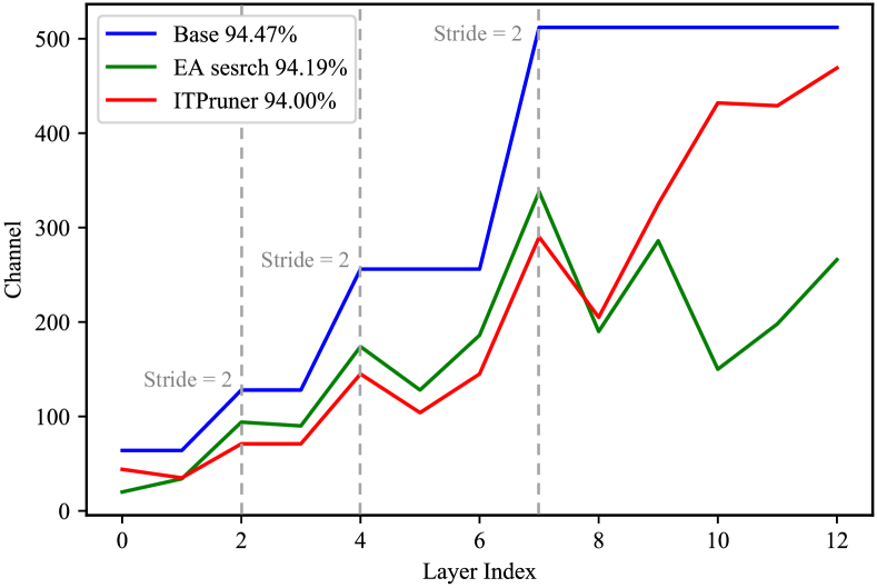
Figure 2: The number of channels for the VGG found by ITPruner (red) and evolutionary algorithm (green). The blue line denotes the uncompressed VGG architecture.

5.3 Ablation Study

In this section, we analyze the architecture found by ITPruner and the influence of the hyper-parameters $\beta$ and $n$. To sum up, the architecture found by ITPruner shows surprisingly similar characteristics compared with the optimal one. Meanwhile, ITPruner is easy to use, i.e., the only two hyper-parameters $\beta$ and $n$ show a negligible performance gap with different values. The detailed experiments are described as follows.

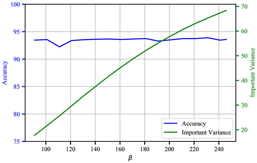
Figure 3: Accuracy (blue) and variance (green) of layer-wise importance in different $\beta$.

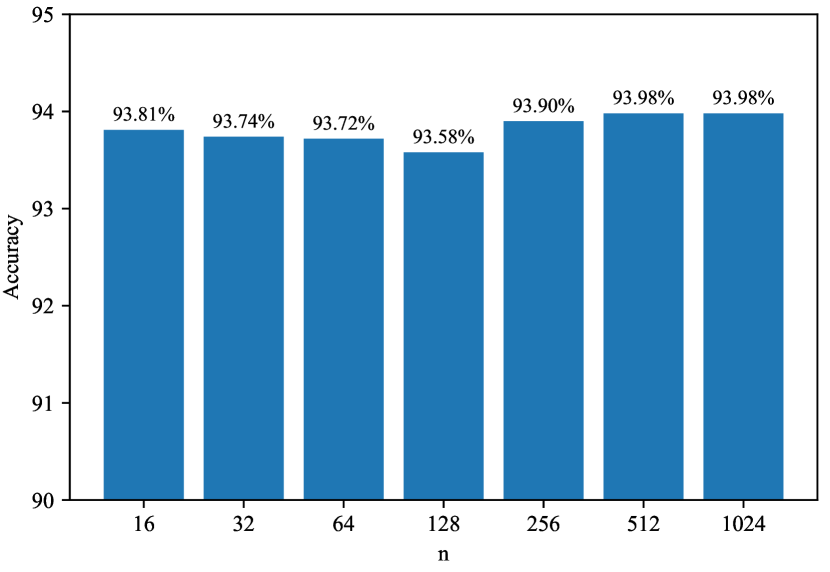
Figure 4: VGG accuracy of layer-wise importance on CIFAR-10 with different $n$.

Architecture analysis. We first adopt Evolutionary Algorithm (EA) [3] to find the optimal architecture, which is employed as a baseline for a better comparison. Specifically, we directly employ the aforementioned training hyper-parameters in the architecture evaluation step. Meanwhile, the search algorithm is executed several times to determine the optimal architecture, which is illustrated in the green line of Fig. 2. Notably, such a process is extremely time-consuming which takes a few GPU days in CIFAR-10. Interestingly, the proposed ITPruner finds architecture that has similar characteristics compared with the optimal architecture. In particular, there are significant peaks in these architectures whenever there is a down sampling operation, i.e., stride $=2$. In such an operation, the resolution is halved thus needs to be compensated by more channels. Similar observations are also reported in MetaPruning [30]. Nevertheless, we do not need any exhausted search process to obtain such insight. We also notice that there is some difference in channel choice between architectures find by ITPruner and EA. That is, ITPruner is prone to assign more channels in the first and the last layers. Meanwhile, the performance gap between these architectures is negligible ($0.19$), which demonstrates the efficiency of our method.

Influence of $\beta$ and $n$. There are only two hyper-parameters in ITPruner. One is the importance factor $\beta$, which is proposed to control relative compression rates between different layers. The other one is sample image $n$, which determines the computation cost of ITPruner. Fig. 3 reports the accuracy and variance of layer-wise importance in different $\beta$. As we can see, layer-wise importance $\boldsymbol{i}$ tends to has a significant variance with a large $\beta$, and vice versa. Such variance finally determines the difference of layer-wise compression rate through Eq. 10. However, the performance gap between different $\beta$ is negligible. Similar results are observed for different $n$. The experiment is available in the supplementary materials. In particular, the variance of top-1 accuracy in CIFAR-10 between different $n$ is around $0.1$. We thus conclude that ITPruner is easy to implement.

We further conduct a experiment to demonstrate the influence of the sample size $n$, which is reported in Fig. 4. As we can see, the variance of the accuracy with different $n$ is 0.1%, which means accuracy will not fluctuate greatly with the change of n and thus demonstrate the robustness of our method.

6 Conclusion

In this paper, we present an information theory-inspired strategy for automatic network pruning (ITPruner), which determines the importance of layer by observing the independence of feature maps and do not need any search process. To that effect, ITPruner is derived from the information bottleneck principle, which proposed to use normalized HSIC to measure and determine the layer-wise compression ratio. We also mathematically prove the robustness of the proposed method as well as the relation to mutual information. Extensive experiments on various modern CNNs demonstrate the effectiveness of ITPruner in reducing the computational complexity and model size. In the future work, we will do more on the theoretical analysis on neural architecture search to effectively find optimal architecture without any search process.

Xiawu Zheng received the M.S. degree in Computer Science, School of Information Science and Engineering, Xiamen University, Xiamen, China, in 2018. He is currently working toward the PH.D. degree at School of Information Science and Engineering, Xiamen University. His research interests include computer vision and machine learning. He was involved in automatic machine learning.

Yuexiao Ma received the B.S. degree in Mathematics and Applied Mathematics, Department of Mathematics, Northeastern University, Shenyang, China, in 2016. He is currently a master student at School of Informatics, Xiamen University. His research interests include machine learning and computer vision. He was involved in neural network quantification.

Teng Xi is a Staff Software Engineer of Computer Vision Department (VIS in short) at Baidu. Previously, he was a joint postdoc researcher in Baidu Inc and Department of Computer Science and Technology at Tsinghua University. He have been awarded the Chinese Government Scholarship for studying abroad, the National Scholarship for Ph.D. students, the BUPT Excellent Ph.D. Students Foundation. His research interest is model compression, Bayesian estimation, and face recognition. He has proposed original NAS algorithms in top-tier conferences/journals such as SA-NAS and GP-NAS. Using the proposed NAS algorithms, he received the 7 Winner prize in competitions of CVPR and ECCV et. He co-organized the Astar 2019 Developer Challenge, the ICML Expo workshop PaddlePaddle-based Deep Learning at Baidu. He organized the CVPR 2021 Neural Architecture Search Workshop and organized the 1st lightweight NAS challenge in CVPR.

Gang Zhang is a Staff Software Engineer of Computer Vision Department (VIS in short) at Baidu. He is leading the team of model compression, automated deep learning, and face recognition. Recently, he has published 6 papers and won competitions such as LPIRC and CFAT in these areas. This year, he also co-organized NAS workshop in CVPR. His team and he are developing both PaddleSlim, a deep learning framework for model compression as well as architecture search, and commercial face recognition systems whose public cloud call has exceeded 100 millions since 2019.

Errui Ding is the director of Computer Vision Department (VIS in short) at Baidu. He has been leading VIS in winning over 30 international academic competitions and releasing over 150 open APIs, thereby helping the public cloud to become the market leader recognized by Forrester and IDC. Meanwhile, he has published over 30 papers and obtained over 50 patents , the best paper runner up award in ICDAR 2019, best manager award at Baidu as well as the First Prize of Science and Technology Award by Chinese Institute of Electronics. In addition, he co-organized 4 workshops and competitions in recent ICDAR and CVPR.

Yuchao Li received the M.S. degree in Computer Science, School of Information Science and Engineering, Xiamen University, Xiamen, China, in 2020. His research interests include computer vision and neural network compression and acceleration.

Jie Chen received his M.S. and Ph.D. degrees from Harbin Institute of Technology, China, in 2002 and 2007, respectively. He joined Peng Cheng Labora- tory, China since 2018. He has been a senior re- searcher in the Center for Machine Vision and Signal Analysis at the University of Oulu, Finland since 2007. In 2012 and 2015, he visited the Computer Vision Laboratory at the University of Maryland and School of Electrical and Computer Engineering at the Duke University respectively. Dr. Chen was a cochair of International Workshops at ACCV, CVPR,and ICCV. He was a guest editor of special issues for IEEE TPAMI and IJCV. His research interests include pattern recognition, computer vision, machine learning, dynamic texture, deep learning, and medical image analysis.

Yonghong Tian is currently the Boya Distinguished Professor of the School of Electronics Engineering and Computer Science, Peking University, China, and also the Deputy Director of the Peng Cheng Laboratory, Artificial Intelligence Research Center, Shenzhen, China. His research interests include computer vision, multimedia big data, and brain-inspired computation. He is the author or coauthor of over 180 technical articles in refereed journals, such as the IEEE TPAMI/TNNLS/TIP/TMM/TCSVT/TKDE/TPDS and the ACM CSUR/TOIS/TOMM and conferences, such as the NeurIPS/CVPR/ICCV/AAAI/ACMMM/WWW. He is a Senior Member of CIE and CCF and a member of ACM. He has been the Steering Member of the IEEE ICME since 2018 and the IEEE International Conference on Multimedia Big Data (BigMM) since 2015, and a TPC Member of more than ten conferences, such as CVPR, ICCV, ACM KDD, AAAI, ACM MM, and ECCV. He was a recipient of the Chinese National Science Foundation for Distinguished Young Scholars in 2018, two National Science and Technology Awards, three Ministerial-Level Awards in China, the 2015 EURASIP Best Paper Award for Journal on Image and Video Processing, and the Best Paper Award of the IEEE BigMM 2018. He was/is an Associate Editor of the IEEE TCSVT since January 2018, the IEEE TMM from August 2014 to August 2018, the IEEE Multimedia Magazine since January 2018, and the IEEE Access since 2017. He also Co-Initiated the BigMM. He has served as the TPC Co-Chair for BigMM 2015 and the Technical Program Co-Chair for the IEEE ICME 2015, the IEEE ISM 2015, and the IEEE MIPR 2018/2019, and the General Co-Chair for the IEEE MIPR 2020

Rongrong Ji is currently a Professor and the Director of the Intelligent Multimedia Technology Laboratory, and the Dean Assistant with the School of Information Science and Engineering, Xiamen University, Xiamen, China. His work mainly focuses on innovative technologies for multimedia signal processing, computer vision, and pattern recognition, with over 100 papers published in international journals and conferences. He is a member of the ACM. He was a recipient of the ACM Multimedia Best Paper Award and the Best Thesis Award of Harbin Institute of Technology. He serves as an Associate/Guest Editor for international journals and magazines such as Neurocomputing, Signal Processing, Multimedia Tools and Applications, the IEEE MultiMedia Magazine, and the Multimedia Systems. He also serves as program committee member for several Tier-1 international conferences.

References

- [1] Sungsoo Ahn, Shell Xu Hu, Andreas Damianou, Neil D Lawrence, and Zhenwen Dai. Variational information distillation for knowledge transfer. In Proceedings of the IEEE/CVF Conference on Computer Vision and Pattern Recognition, pages 9163–9171, 2019.
- [2] Alexander A Alemi, Ian Fischer, Joshua V Dillon, and Kevin Murphy. Deep variational information bottleneck. arXiv preprint arXiv:1612.00410, 2016.
- [3] Thomas Back. Evolutionary Algorithms in Theory and Practice: Evolution Strategies, Evolutionary Programming, Genetic algorithms. 1996.
- [4] Davis Blalock, Jose Javier Gonzalez Ortiz, Jonathan Frankle, and John Guttag. What is the state of neural network pruning? arXiv preprint arXiv:2003.03033, 2020.
- [5] L. Chen, G. Papandreou, I. Kokkinos, K. Murphy, and A. L. Yuille. Deeplab: Semantic image segmentation with deep convolutional nets, atrous convolution, and fully connected crfs. IEEE transactions on pattern analysis and machine intelligence (TPAMI), 2018.
- [6] Thomas M Cover. Elements of information theory. John Wiley & Sons, 1999.
- [7] Bin Dai, Chen Zhu, Baining Guo, and David Wipf. Compressing neural networks using the variational information bottleneck. In International Conference on Machine Learning, pages 1135–1144. PMLR, 2018.
- [8] Xuanyi Dong and Yi Yang. Network pruning via transformable architecture search. Advances in Neural Information Processing Systems, 2019.
- [9] W. N. Everitt. A note on positive definite matrices. Proceedings of the Glasgow Mathematical Association, 3(4):173–175, 1958.
- [10] Ross Girshick. Fast r-cnn. In International Conference on Computer Vision (ICCV), 2015.
- [11] Z Goldfeld, E van den Berg, K Greenewald, I Melnyk, N Nguyen, B Kingsbury, and Y Polyanskiy. Estimating information flow in neural networks. arxiv e-prints, page. arXiv preprint arXiv:1810.05728, 2018.
- [12] Arthur Gretton, Olivier Bousquet, Alex Smola, and Bernhard Schölkopf. Measuring statistical dependence with hilbert-schmidt norms. In International conference on algorithmic learning theory, pages 63–77. Springer, 2005.
- [13] Kaiming He, Xiangyu Zhang, Shaoqing Ren, and Jian Sun. Deep residual learning for image recognition. In Computer Vision and Pattern Recognition (CVPR), 2016.
- [14] Yihui He, Ji Lin, Zhijian Liu, Hanrui Wang, Li-Jia Li, and Song Han. Amc: Automl for model compression and acceleration on mobile devices. In Proceedings of the European Conference on Computer Vision (ECCV), pages 784–800, 2018.
- [15] Yang He, Ping Liu, Ziwei Wang, Zhilan Hu, and Yi Yang. Filter pruning via geometric median for deep convolutional neural networks acceleration. In Proceedings of the IEEE Conference on Computer Vision and Pattern Recognition, pages 4340–4349, 2019.
- [16] Andrew Howard, Mark Sandler, Grace Chu, Liang-Chieh Chen, Bo Chen, Mingxing Tan, Weijun Wang, Yukun Zhu, Ruoming Pang, Vijay Vasudevan, et al. Searching for mobilenetv3. In Proceedings of the IEEE/CVF International Conference on Computer Vision, pages 1314–1324, 2019.
- [17] Andrew G Howard, Menglong Zhu, Bo Chen, Dmitry Kalenichenko, Weijun Wang, Tobias Weyand, Marco Andreetto, and Hartwig Adam. Mobilenets: Efficient convolutional neural networks for mobile vision applications. arXiv preprint arXiv:1704.04861, 2017.
- [18] Sergey Ioffe and Christian Szegedy. Batch normalization: Accelerating deep network training by reducing internal covariate shift. In International conference on machine learning, pages 448–456. PMLR, 2015.
- [19] Benoit Jacob, Skirmantas Kligys, Bo Chen, Menglong Zhu, Matthew Tang, Andrew Howard, Hartwig Adam, and Dmitry Kalenichenko. Quantization and training of neural networks for efficient integer-arithmetic-only inference. Computer Vision and Pattern Recognition (CVPR), 2018.
- [20] Simon Kornblith, Mohammad Norouzi, Honglak Lee, and Geoffrey Hinton. Similarity of neural network representations revisited. In International Conference on Machine Learning, pages 3519–3529. PMLR, 2019.
- [21] Dieter Kraft et al. A software package for sequential quadratic programming. 1988.
- [22] Alex Krizhevsky, Ilya Sutskever, and Geoffrey E Hinton. Imagenet classification with deep convolutional neural networks. Advances in neural information processing systems, 2012.
- [23] Yann LeCun, Yoshua Bengio, and Geoffrey Hinton. Deep learning. nature, 2015.
- [24] Yann LeCun, Léon Bottou, Yoshua Bengio, Patrick Haffner, et al. Gradient-based learning applied to document recognition. Proceedings of the IEEE, 1998.
- [25] Hao Li, Asim Kadav, Igor Durdanovic, Hanan Samet, and Hans Peter Graf. Pruning filters for efficient convnets. International Conference on Learning Representations (ICLR), 2016.
- [26] Mingbao Lin, Rongrong Ji, Yan Wang, Yichen Zhang, Baochang Zhang, Yonghong Tian, and Ling Shao. Hrank: Filter pruning using high-rank feature map. IEEE Conference on Computer Vision and Pattern Recognition, 2020.
- [27] Mingbao Lin, Rongrong Ji, Yuxin Zhang, Baochang Zhang, Yongjian Wu, and Yonghong Tian. Channel pruning via automatic structure search.
- [28] Shaohui Lin, Rongrong Ji, Yuchao Li, Yongjian Wu, Feiyue Huang, and Baochang Zhang. Accelerating convolutional networks via global & dynamic filter pruning. In IJCAI, pages 2425–2432, 2018.
- [29] Shaohui Lin, Rongrong Ji, Chenqian Yan, Baochang Zhang, Liujuan Cao, Qixiang Ye, Feiyue Huang, and David Doermann. Towards optimal structured cnn pruning via generative adversarial learning. In Proceedings of the IEEE Conference on Computer Vision and Pattern Recognition, pages 2790–2799, 2019.
- [30] Zechun Liu, Haoyuan Mu, Xiangyu Zhang, Zichao Guo, Xin Yang, Kwang-Ting Cheng, and Jian Sun. Metapruning: Meta learning for automatic neural network channel pruning. In Proceedings of the IEEE/CVF International Conference on Computer Vision, pages 3296–3305, 2019.
- [31] Zhuang Liu, Mingjie Sun, Tinghui Zhou, Gao Huang, and Trevor Darrell. Rethinking the value of network pruning. In International Conference on Learning Representations, 2018.
- [32] Jonathan Long, Evan Shelhamer, and Trevor Darrell. Fully convolutional networks for semantic segmentation. In Computer Vision and Pattern Recognition (CVPR), 2015.
- [33] Urbano Lorenzo-Seva and Jos MF Ten Berge. Tucker’s congruence coefficient as a meaningful index of factor similarity. Methodology, 2(2):57–64, 2006.
- [34] Jian-Hao Luo, Jianxin Wu, and Weiyao Lin. Thinet: A filter level pruning method for deep neural network compression. International Conference on Computer Vision (ICCV), 2017.
- [35] Wan-Duo Kurt Ma, JP Lewis, and W Bastiaan Kleijn. The hsic bottleneck: Deep learning without back-propagation. In Proceedings of the AAAI Conference on Artificial Intelligence, volume 34, pages 5085–5092, 2020.
- [36] Pavlo Molchanov, Arun Mallya, Stephen Tyree, Iuri Frosio, and Jan Kautz. Importance estimation for neural network pruning. In Proceedings of the IEEE Conference on Computer Vision and Pattern Recognition, 2019.
- [37] Pavlo Molchanov, Arun Mallya, Stephen Tyree, Iuri Frosio, and Jan Kautz. Importance estimation for neural network pruning. In Proceedings of the IEEE/CVF Conference on Computer Vision and Pattern Recognition, pages 11264–11272, 2019.
- [38] Adam Paszke, Sam Gross, Soumith Chintala, Gregory Chanan, Edward Yang, Zachary DeVito, Zeming Lin, Alban Desmaison, Luca Antiga, and Adam Lerer. Automatic differentiation in pytorch. 2017.
- [39] S. Ren, K. He, R. Girshick, and J. Sun. Faster r-cnn: Towards real-time object detection with region proposal networks. IEEE transactions on pattern analysis and machine intelligence (TPAMI), 2017.
- [40] Paul Robert and Yves Escoufier. A unifying tool for linear multivariate statistical methods: The rv-coefficient. Journal of the Royal Statistical Society: Series C (Applied Statistics), 25(3):257–265, 1976.
- [41] Olga Russakovsky, Jia Deng, Hao Su, Jonathan Krause, Sanjeev Satheesh, Sean Ma, Zhiheng Huang, Andrej Karpathy, Aditya Khosla, Michael Bernstein, et al. Imagenet large scale visual recognition challenge. IJCV, 2015.
- [42] Mark Sandler, Andrew Howard, Menglong Zhu, Andrey Zhmoginov, and Liang-Chieh Chen. Mobilenetv2: Inverted residuals and linear bottlenecks. In Proceedings of the IEEE conference on computer vision and pattern recognition, pages 4510–4520, 2018.
- [43] Ravid Shwartz-Ziv and Naftali Tishby. Opening the black box of deep neural networks via information. CoRR, 2017.
- [44] Karen Simonyan and Andrew Zisserman. Very deep convolutional networks for large-scale image recognition. arXiv preprint arXiv:1409.1556, 2014.
- [45] Mingxing Tan, Bo Chen, Ruoming Pang, Vijay Vasudevan, Mark Sandler, Andrew Howard, and Quoc V Le. Mnasnet: Platform-aware neural architecture search for mobile. In Proceedings of the IEEE/CVF Conference on Computer Vision and Pattern Recognition, pages 2820–2828, 2019.
- [46] Mingxing Tan and Quoc Le. Efficientnet: Rethinking model scaling for convolutional neural networks. In International Conference on Machine Learning, pages 6105–6114. PMLR, 2019.
- [47] Naftali Tishby, Fernando C. Pereira, and William Bialek. The information bottleneck method. In Proc. of the 37-th Annual Allerton Conference on Communication, Control and Computing, 1999.
- [48] Jiaxing Wang, Haoli Bai, Jiaxiang Wu, Xupeng Shi, Junzhou Huang, Irwin King, Michael Lyu, and Jian Cheng. Revisiting parameter sharing for automatic neural channel number search. Advances in Neural Information Processing Systems, 33, 2020.
- [49] Jiayun Wang, Yubei Chen, Rudrasis Chakraborty, and Stella X Yu. Orthogonal convolutional neural networks. In Proceedings of the IEEE/CVF Conference on Computer Vision and Pattern Recognition, pages 11505–11515, 2020.
- [50] Wei Wen, Chunpeng Wu, Yandan Wang, Yiran Chen, and Hai Li. Learning structured sparsity in deep neural networks. Advances in Neural Information Processing Systems (NeurIPS), 2016.
- [51] Tien-Ju Yang, Andrew Howard, Bo Chen, Xiao Zhang, Alec Go, Mark Sandler, Vivienne Sze, and Hartwig Adam. Netadapt: Platform-aware neural network adaptation for mobile applications. In Proceedings of the European Conference on Computer Vision (ECCV), pages 285–300, 2018.
- [52] Jiahui Yu and Thomas Huang. Autoslim: Towards one-shot architecture search for channel numbers. arXiv preprint arXiv:1903.11728, 2019.
- [53] Shuchang Zhou, Yuxin Wu, Zekun Ni, Xinyu Zhou, He Wen, and Yuheng Zou. Dorefa-net: Training low bitwidth convolutional neural networks with low bitwidth gradients. Computer Vision and Pattern Recognition (CVPR), 2016.