Quantized edge magnetizations and their symmetry protection
in one-dimensional quantum spin systems

Abstract

The bulk electric polarization works as a nonlocal order parameter that characterizes topological quantum matters. Motivated by a recent paper [H. Watanabe et al., Phys. Rev. B 103, 134430 (2021)], we discuss magnetic analogs of the bulk polarization in one-dimensional quantum spin systems, that is, quantized magnetizations on the edges of one-dimensional quantum spin systems. The edge magnetization shares the topological origin with the fractional edge state of the topological odd-spin Haldane phases. Despite this topological origin, the edge magnetization can also appear in topologically trivial quantum phases. We develop straightforward field theoretical arguments that explain the characteristic properties of the edge magnetization. The field theory shows that a U(1) spin-rotation symmetry and a site-centered or bond-centered inversion symmetry protect the quantization of the edge magnetization. We proceed to discussions that quantum phases on nonzero magnetization plateaus can also have the quantized edge magnetization that deviates from the magnetization density in bulk. We demonstrate that the quantized edge magnetization distinguishes two quantum phases on a magnetization plateau separated by a quantum critical point. The edge magnetization exhibits an abrupt stepwise change from zero to $1/2$ at the quantum critical point because the quantum phase transition occurs in the presence of the symmetries protecting the quantization of the edge magnetization. We also show that the quantized edge magnetization can result from the spontaneous ferrimagnetic order.

I Introduction

The electric polarization is a fundamental object of electromagnetism Landau et al. (2013). The polarization also receives attention to its close connection with topological quantum matters. Even though intrinsic to the bulk, the electric polarization manifests itself as an accumulation of charges on the surface Vanderbilt and King-Smith (1993). Surface electric charges work as topological indices of topological insulators and higher-order ones Benalcazar et al. (2017a, b); Qi et al. (2008); Ezawa (2018). Importantly, we can experimentally access the surface charge more easily than the entanglement entropies and spectra Pollmann et al. (2010, 2012) and other related nonlocal order parameters Affleck et al. (1988); Kennedy and Tasaki (1992); Kohmoto and Tasaki (1992); Nakamura and Todo (2002).

Considering the fruitful relations between the surface charges and topological quantum matters, we can expect that it holds promise to consider a magnetic analog of the surface electric charge. A leading candidate is a surface magnetization because the magnetization is a conserved quantity associated with a global U(1) symmetry similarly to the electric charge. Recently, Watanabe et al. Watanabe et al. (2021) found fractionally quantized magnetizations, $M^{z}=\pm S/2^{d}$, accumulated on edges ($d=1$) or corners ($d=2,3$) of $d$-dimensional cubic-lattice Heisenberg antiferromagnetic (HAFM) models under a staggered magnetic field. They showed that these fractional edge and corner magnetizations qualify as the magnetic analog of the bulk polarization.

We can expect that the edge or corner magnetization will detect some topological properties of quantum magnets. Reference Watanabe et al. (2021) suggested that the edge magnetization $M^{z}=\pm 1/2$ in the spin-1 chain is “reminiscent of the $S=1/2$ edge mode” of the spin-1 Haldane phase. On the other hand, the edge magnetization also emerges in topologically trivial phases such as the forced Néel phase of the spin-$1/2$ chain.

However, it is still puzzling what kind of topological property the edge magnetization detects. The two spin chains mentioned above seem to have different topological profiles. The topological aspect of the edge magnetization as the bulk polarization is nontrivial even in one-dimensional systems, which is worth further investigations, in particular, from a field-theoretical point of view. One-dimensional quantum theories will be useful to build two- or three-dimensional quantum states with quantized corner magnetizations Watanabe et al. (2021) similarly to coupled-wire constructions of topological states Kane et al. (2002); Teo and Kane (2014); Meng et al. (2015); Lecheminant and Tsvelik (2017).

This paper develops a quantum field theory of the edge magnetization as the magnetic analog of the bulk electric polarization. We make twofold claims. One is that the quantum field theory clarifies that the symmetry-protected edge state of the topological Haldane phase and the quantized edge magnetization of the topologically trivial phase have the same origin. They originate from a zero mode of a nonlocal boson field whose spatial gradient represents the magnetization density. The other is that the edge magnetization also appears in quantum spin systems in uniform magnetic fields. The staggered magnetic field is not always necessary to induce the quantized edge magnetization. The quantized edge magnetization can be induced by spatially modulated exchange interactions and even by spatially uniform interactions.

We organize this paper to make it accessible to a broad readership without going deeply into technical details of quantum field theories, while details are given in Appendices to make the paper self-contained. We first give a field-theoretical interpretation of the quantized edge magnetization in the general spin-$S$ HAFM chains (Sec. II), where we see the physical meaning of the Gaussian convolution introduced in Ref. Watanabe et al. (2021). Next, we apply the magnetic field to quantum spin systems. Section III deals with a $1/2$ magnetization plateau of the spin ladder, where we arrive at a generalized definition of the edge magnetization valid on the magnetization plateaus. Sections IV and V also discuss edge magnetizations on the magnetization plateaus, but their ground states are much more nontrivial than that dealt with in Sec. III. We will see an interesting topological quantum phase transition on the 1/2 magnetization plateau accompanied by an abrupt change of the edge magnetizations and the total charge in Sec. IV. Section V discusses the ferrimagnetic ground state with the edge magnetization. We summarize the paper in Sec. VI. Appendices describe details of quantum field theories. Note that Appendices B and C contain novel results such as what we call “semiclassical bosonization formulas”.

II Unification of topological edge state and edge magnetization

II.1 Quantized edge magnetization in topologically trivial phase of spin-1/2 chain

We start our discussions by field-theoretically interpreting results of Ref. Watanabe et al. (2021) for one-dimensional systems. The simplest situation is the spin-$1/2$ HAFM chain with the staggered magnetic field. The Hamiltonian with the open boundary condition (OBC) is given by

$$\mathcal{H}=J\sum_{j=1}^{L-1}\bm{S}_{j}\cdot\bm{S}_{j+1}+h_{s}\sum_{j=1}^{L}(-1)^{j}S_{j}^{z},$$ (1)

where $\bm{S}_{j}$ is the spin-$1/2$ operator at the $j$th site and $J>0$ is the antiferromagnetic exchange coupling and $h_{s}>0$ is the staggered magnetic field. According to the Marshall-Lieb-Mattis theorem Marshall (1955); Lieb and Mattis (1962), the ground state of the model (1) satisfies

$$\sum_{j=1}^{L}\braket{S_{j}^{z}}=0.$$ (2)

If we regard $S_{j}^{z}$ as a charge, Eq. (2) gives a charge neutrality condition. Precisely speaking, the neutrality condition (2) is met only when $L$ is even. We assume even $L$ throughout this paper.

The low-energy physics of this spin chain is described by a quantum field theory of an interacting U(1) compactified boson $\phi$ with a trigonometric potential, called the sine-Gordon theory Giamarchi (2004); Gogolin et al. (2004):

$$\mathcal{H}_{s} =\int_{0}^{L}dx\biggl{[}\frac{v}{2\pi K}(\partial_{\mu}\phi)^{2}+g_{s}\sin(2\phi)\biggr{]}.$$ (3)

Hereafter, we employ a unit system with $\hbar=a_{0}=1$ ($a_{0}$ is the lattice spacing) for simplicity, but will call $a_{0}$ back whenever we need. The first term of Eq. (3) is the kinetic term, where $(\partial_{\mu}\phi)^{2}=v^{-2}(\partial_{\tau}\phi)^{2}+(\partial_{x}\phi)^{2}$ and $x$ and $\tau$ are the space and the imaginary time, respectively. This paper mainly uses the imaginary-time formalism for later convenience. The coupling of the sine potential is proportional to the staggered field, $g_{s}\propto h_{s}$ . The parameter $v$ denotes the velocity of the boson field, $\phi$ Giamarchi (2004). For the spin-1/2 Heisenberg chain, $v=\pi J/2$ Giamarchi (2004). The $\phi$ field is related to the spin operator $\bm{S}_{j}$ as Giamarchi (2004); Gogolin et al. (2004)

$$\bm{S}_{j}=\bm{M}_{j}+(-1)^{j}\bm{N}_{j}$$ (4)

where the $z$ component is given by

$$M_{j}^{z}=\frac{a_{0}}{\pi}\partial_{x}\phi,\qquad N_{j}^{z}=a_{1}\sin(2\phi),$$ (5)

with a constant $a_{1}$ Hikihara and Furusaki (2004). If $h_{s}=0$, the ground state of the spin-1/2 HAFM chain (1) is the gapless Tomonaga-Luttinger (TL) liquid state Giamarchi (2004); Gogolin et al. (2004) governed by the kinetic term, $v(\partial_{\mu}\phi)^{2}/2\pi K$. The sine potential, $\sin(2\phi)$, favoring a constant $\phi$ competes with the kinetic term favoring a constant $\partial_{\mu}\phi$. The staggered magnetic field $h_{s}$ yields the spin gap by locking the $\phi$ field to a minimum of the sine potential,

$$\bar{\phi}=-\frac{\pi}{4}\mod\pi.$$ (6)

In one-dimensional quantum many-body systems, the bulk polarization $\mathcal{P}$ is precisely given by the Resta’s formula Resta (1998); Watanabe and Oshikawa (2018),

$$\mathcal{P} =\frac{1}{2\pi}\operatorname{Im}\ln\braket{U}.$$ (7)

Resta gave $U=\exp(i\frac{2\pi}{L}\sum_{j=1}^{L}jn_{j})$ with the one-particle density $n_{j}$ Resta (1998). In quantum spin systems, $S_{j}^{z}$ plays the role of $n_{j}$ Giamarchi (2004); Watanabe et al. (2021). Hence, we here define $U$ as

$$U =\exp\biggl{(}i\frac{2\pi}{L}\sum_{j=1}^{L}jS_{j}^{z}\biggr{)},$$ (8)

in the model (1). The nonlocal operator (8) is deeply related to the Lieb-Schultz-Mattis (LSM) theorem Lieb et al. (1961); Oshikawa (2000); Oshikawa et al. (1997); Yao and Oshikawa (2020) that allows for classification of gapless quantum phases Cho et al. (2017); Furuya and Oshikawa (2017); Yao et al. (2019). The ground state expectation value $\braket{U}$ is called the polarization amplitude and was previously studied in valence-bond-solid phases Nakamura and Todo (2002) and in the TL-liquid phase Kobayashi et al. (2018); Nakamura and Furuya (2019); Furuya and Nakamura (2019).

The bosonization formula $M_{j}^{z}=\partial_{x}\phi/\pi$ gives Furuya and Nakamura (2019)

$$U =\exp[2i(\phi(L)-\bar{\phi})],$$ (9)

$$\bar{\phi} =\frac{1}{L}\int_{0}^{L}dx\,\phi(x),$$ (10)

where $\bar{\phi}$ is the zero mode of the $\phi$ boson Giamarchi (2004). $\bar{\phi}$ can also be seen as the spatial average of $\phi$. The representation (9) implies that $\phi(L)$ at the right edge of the chain deviates from the average $\bar{\phi}$ when $\mathcal{P}\not=0$. The field $\phi(x=0)$ at the left edge also deviates from $\bar{\phi}$ because the OBC on the spin chain imposes the following boundary condition on $\phi(x)$ Eggert and Affleck (1992) (Appendix A):

$$\phi(0)=\phi(L)=0\mod\pi.$$ (11)

The lockings (11) of $\phi$ at the edges hold irrespective of the locking (6) in the bulk. The boundary condition (11) holds even when the bulk is gapless. The boundary condition (11) is automatically consistent with the charge neutrality because $\sum_{j=1}^{L}\braket{S_{j}^{z}}=\braket{(\phi(L)-\phi(0))}/\pi=0$. Equation (11) also indicates that $\bar{\phi}$ generally represents the locking position of $\phi$ in the bulk. With the OBC, the polarization amplitude $\braket{U}$ is thus given by

$$\braket{U}=\braket{e^{-2i\bar{\phi}}}\approx e^{-2i\braket{\bar{\phi}}}.$$ (12)

Note that the latter approximate equality holds when a relevant interaction strongly locks $\phi$ in bulk to a constant. The approximation becomes more accurate when the bulk excitation gap due to the staggered field becomes larger. We thus find that the bulk polarization (7) is given by the zero mode,

$$\mathcal{P}\approx-\frac{1}{\pi}\braket{\bar{\phi}}\mod 1,$$ (13)

since $\phi$ is real [see Eq. (5)].

The staggered magnetic field leads to the locking (6) of $\bar{\phi}$. Hence, the bulk polarization $\mathcal{P}=1/4\mod 1$ follows. The locking value $\phi(L)=0$ at the right edge $x=L$ indeed deviates from the bulk one (6).

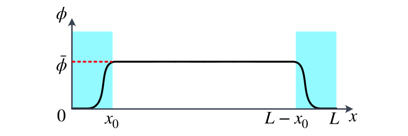
Figure 1: Schematic $x$ dependence of $\phi(x)$ of sine-Gordon model (3). The shaded areas depict the left and right edges, $\mathcal{L}$ and $\mathcal{R}$.

We can relate the bulk polarization $\mathcal{P}$ and the edge magnetization introduced by Ref. Watanabe et al. (2021) as follows. It is generally not obvious how to clearly distinguish the bulk from the edge. There is no clear border between the bulk and the edge. However, when $\bar{\phi}\not=0\mod\pi$, we can distinguish the bulk and the edge by setting a sufficiently small cutoff $\epsilon>0$. Let us define the bulk part, $\mathcal{B}$, of the spin chain as a region where $\phi(x)$ is locked to $\bar{\phi}$,

$$\mathcal{B} =\{x\in[0,L]\,|\,0\leq|\phi(x)-\bar{\phi}|<\epsilon\mod\pi\}.$$ (14)

It is convenient to split $\mathcal{B}=\mathcal{B}_{l}\cup\mathcal{B}_{r}$ into two:

$$\mathcal{B}_{l} =\{x\in[0,L/2]\,|\,0\leq|\phi(x)-\bar{\phi}|<\epsilon\mod\pi\},$$ (15)

$$\mathcal{B}_{r} =\{x\in(L/2,L]\,|\,0\leq|\phi(x)-\bar{\phi}|<\epsilon\mod\pi\}.$$ (16)

The left edge $\mathcal{L}$ and the right edge $\mathcal{R}$ are then defined as

$$\mathcal{L} =[0,\,L/2]\setminus\mathcal{B}_{l},$$ (17)

$$\mathcal{R} =(L/2,\,L]\setminus\mathcal{B}_{r},$$ (18)

where $\setminus$ denotes the set difference. We can rewrite $\mathcal{L}=[0,x_{0})$ and $\mathcal{R}=(L-x_{0},L]$ by using the smallest $x_{0}\in\mathcal{B}$ (the shaded areas of Fig. 1). Then, the uniform part, $M_{j}^{z}$, of $S_{j}^{z}$ on the left edge $\mathcal{L}$ corresponds to $-\mathcal{P}$ because

$$\sum_{ja_{0}\in\mathcal{L}}\braket{M_{j}^{z}} =\int_{x\in\mathcal{L}}dx\,\frac{1}{\pi}\braket{\partial_{x}\phi(x)}$$

$$=\frac{1}{\pi}\braket{[\phi(x_{0})-\phi(0)]}$$

$$\approx-\mathcal{P}+O(\epsilon).$$ (19)

Likewise, we obtain on the right edge,

$$\sum_{ja_{0}\in\mathcal{R}}\braket{M_{j}^{z}} =\int_{x\in\mathcal{R}}dx\,\frac{1}{\pi}\braket{\partial_{x}\phi(x)}$$

$$=\frac{1}{\pi}\braket{[\phi(L)-\phi(L-x_{0})]}$$

$$\approx\mathcal{P}+O(\epsilon).$$ (20)

Hence, we find that Eqs (19) and (20) equal to the quantized edge magnetizations reported in Ref. Watanabe et al. (2021).

To further support this claim, we recall the definition of the edge magnetization by Watanabe et al. Watanabe et al. (2021). They first convoluted a Gaussian function,

$$g(r)=\frac{1}{\sqrt{2\pi\lambda^{2}}}\exp\biggl{(}-\frac{r^{2}}{2\lambda^{2}}\biggr{)},$$ (21)

with $\lambda>0$ to the magnetization $\braket{S_{r}^{z}}$:

$$m^{z}(r)=\sum_{r^{\prime}=1}^{L}g(r-r^{\prime})\braket{S_{r^{\prime}}^{z}}.$$ (22)

Next, they defined the edge magnetizations on both edges by using the convoluted magnetization (22).

$$M_{\rm left}^{z}=\int_{-\infty}^{\frac{L+1}{2}}dr\,m^{z}(r),\quad M_{\rm right}^{z}=\int_{\frac{L+1}{2}}^{\infty}dr\,m^{z}(r).$$ (23)

The rapid oscillation $(-1)^{j}$ over the finite Gaussian window suppresses the staggered component $N_{j}^{z}$’s contribution to $m^{z}(r)$. We can rewrite $M_{\rm left}^{z}$ as

$$M_{\rm left}^{z} =\int_{0}^{L}dr^{\prime}\,\frac{1}{\pi}\braket{\partial_{r^{\prime}}\phi(r^{\prime})}\int_{-\infty}^{\frac{L+1}{2}}dr\,g(r-r^{\prime}).$$ (24)

The integral about $r$ approximately gives

$$\int_{-\infty}^{\frac{L+1}{2}}dr\,g(r-r^{\prime}) \approx\left\{\begin{array}[]{ccc}1&&(\text{for }r^{\prime}\lesssim\tfrac{L+1}{2}+\lambda)\\ &&\\ 0&&(\text{otherwise})\end{array}\right.$$ (28)

Therefore, $M_{\rm left}^{z}$ is reduced to

$$M_{\rm left}^{z} \approx\int_{-\infty}^{\frac{L+1}{2}+\lambda}dr^{\prime}\,\frac{1}{\pi}\braket{\partial_{r^{\prime}}\phi(r^{\prime})}$$

$$=\frac{1}{\pi}\biggl{\langle}\biggl{(}\phi\biggl{(}\frac{L+1}{2}+\lambda\biggr{)}-\phi(0)\biggr{)}\biggr{\rangle}$$

$$=\frac{1}{\pi}\bar{\phi}$$

$$\approx-\mathcal{P}.$$ (29)

By applying a similar procedure to $M_{\rm right}^{z}$, we obtain

$$M_{\rm left}^{z} \approx\sum_{ja_{0}\in\mathcal{L}}\braket{M_{j}^{z}}\approx-\mathcal{P},$$ (30)

$$M_{\rm right}^{z} \approx\sum_{ja_{0}\in\mathcal{R}}\braket{M_{j}^{z}}\approx\mathcal{P},$$ (31)

We can employ any other smooth normalized window function $g(r)$ (e.g. Lorentzian). Regardless of the details or choice of $g(r)$, the convolution (22) with the finite window function $g(r)$ discards the staggered part of $S_{j}^{z}$. Equations (30) and (31) become more accurate as the lowest excitation gap in the bulk becomes larger. Indeed, Ref. Watanabe et al. (2021) demonstrated that the edge magnetizations $M_{\rm left}^{z}$ and $M_{\rm right}^{z}$ rapidly approach $-\mathcal{P}$ and $+\mathcal{P}$ respectively as the bulk excitation gap grows.

II.2 Topological edge state and quantized edge magnetization in topological phase of spin-1 chain

The sine-Gordon argument also applies to the spin-$1$ HAFM chain. When the topological properties are concerned, we may identify the spin-$1$ HAFM chain as a two-leg spin-$1/2$ ladder with a weak ferromagnetic interchain interaction Schulz (1986); Kim et al. (2000); Hijii et al. (2005),

$$\mathcal{H}_{\rm ladder} =J\sum_{j=1}^{L-1}\sum_{n=1,2}\bm{S}_{j,n}\cdot\bm{S}_{j+1,n}+J_{\perp}\sum_{j=1}^{L}\bm{S}_{j,1}\cdot\bm{S}_{j,2},$$ (32)

where each leg labeled by $n=1,2$ is the spin-$1/2$ HAFM chain and corresponds to the TL liquid of a boson $\phi_{n}$. It is numerically confirmed that the weak ferromagnetic rung region ($-J_{\perp}/J\ll 1$) is adiabatically connected to the strong rung limit $-J_{\perp}/J\to-\infty$, that is, the spin-1 HAFM chain Hijii et al. (2005).

The low-energy effective Hamiltonian is again the sine-Gordon theory (3) of a boson, $\phi=\phi_{1}+\phi_{2}$ Shelton et al. (1996); Chitra and Giamarchi (1997),

$$\mathcal{H}_{\mathrm{c}} =\int_{0}^{L}dx\biggl{[}\frac{v}{2\pi K}(\partial_{\mu}\phi)^{2}+g_{c}\cos(2\phi)\biggr{]}.$$ (33)

This time, the trigonometric potential appears even in the absence of the staggered field. The coupling $g_{c}\propto-J_{\perp}$ is proportional to the ferromagnetic rung interaction, $J_{\perp}<0$ Shelton et al. (1996). If we impose the charge neutrality condition,

$$\sum_{j=1}^{L}\sum_{n=1,2}\braket{S_{j,n}^{z}}=0,$$ (34)

on the $\phi$ field, we obtain the OBC,

$$\phi(0)=\phi(L)=0\mod\pi,$$ (35)

in analogy with the spin-$1/2$ chain.

The ferromagnetic rung interaction locks $\bar{\phi}=\pm\pi/2\mod\pi$, leading to $\mathcal{P}=\mp 1/2\mod 1$. On the other hand, the antiferromagnetic coupling $J_{\perp}>0$ (i.e. $g_{c}<0$) locks $\bar{\phi}=0\mod\pi$, leading to $\mathcal{P}=0\mod 1$. The bulk polarization $\mathcal{P}$ thus distinguishes the topological Haldane phase for $J_{\perp}<0$ and the topologically trivial (rung-singlet) phase for $J_{\perp}>0$.

Similarly to the spin-$1/2$ chain with the staggered field, the spin-$1$ HAFM chain is accompanied by the bulk polarization $\mathcal{P}=\mp 1/2$ that corresponds to the spin-$1/2$ edge state of the symmetry-protected topological spin-$1$ Haldane phase. Unlike the spin-$1/2$ chain, the edge state is degenerate, and the degeneracy is protected by a symmetry such as a bond-centered inversion symmetry Pollmann et al. (2010, 2012). The sine-Gordon theory (33) indicates that the ground state is doubly degenerate, $\ket{\rm GS_{\pm}}=(\ket{\psi_{+}}\pm\ket{\psi_{-}})/\sqrt{2}$. Here, $\ket{\psi_{\pm}}$ denote bulk quantum states accompanied by edge magnetizations $(M_{\rm left}^{z},\,M_{\rm right}^{z})=(\mp 1/2,\,\pm 1/2)$, respectively. In other words, $\ket{\psi_{\pm}}$ corresponds to a state with $\bar{\phi}=\mp\pi/2$, respectively. We regard their superpositions, $\ket{\rm GS_{\pm}}$, as the degenerate ground states because $\ket{\psi_{\pm}}$ are not eigenstates of a bond-centered inversion $\mathcal{I}_{b}:\bm{S}_{j}\to\bm{S}_{L+1-j}$ but $\ket{\rm GS_{\pm}}$ are. The bond-centered inversion acts on $\phi_{1}$ and $\phi_{2}$ as

$$\mathcal{I}_{b}\phi_{n}(x)\mathcal{I}_{b}^{-1} =-\phi_{n}(L-x)\mod\pi.$$ (36)

Accordingly, $\phi(x)=\phi_{1}(x)+\phi_{2}(x)$ transforms as

$$\mathcal{I}_{b}\phi(x)\mathcal{I}_{b}^{-1} =-\phi(L-x)\mod\pi.$$ (37)

Since $\bar{\phi}$ represents the locking position of $\phi$ in the bulk, $\mathcal{I}_{b}$ transforms $\bar{\phi}=\pi/2$ to $\bar{\phi}=-\pi/2\mod\pi$ and vice versa. Hence, it follows that $\mathcal{I}_{b}\ket{\psi_{\pm}}=\ket{\psi_{\mp}}$ and $\mathcal{I}_{b}\ket{\rm GS_{\pm}}=\pm\ket{\rm GS_{\pm}}$. Whereas $\ket{\psi_{\pm}}$ is accompanied by the nonzero quantized magnetization, $\ket{\rm GS_{\pm}}$ are not.

Note that we found twofold degeneracy, not the fourfold one. The ground state in the spin-1 Haldane phase with the OBC is fourfold degenerate because each end of the spin chain hosts the fractionalized $S=1/2$ spin. This difference in the ground-state degeneracy originates from the charge neutrality condition (34). Among the four ground states of the spin-1 HAFM chain with the OBC, two ground states live in the charge-neutral sector (34) but the other two live out of it. The sine-Gordon theory (33) formulated on the basis of the charge neutrality condition (34) thus predicts the twofold degeneracy. The sine-Gordon theory gives the other two ground states of the spin-1 Haldane phase if we impose boundary conditions, $(\phi(0),\phi(L))=(0,\pi)$ or $(\phi(0),\phi(L))=(\pi,0)$. The former boundary condition gives $(M_{\rm left}^{z},M_{\rm right}^{z})=(1/2,1/2)$ and the latter gives $(M_{\rm left}^{z},M_{\rm right}^{z})=(-1/2,-1/2)$.

We derived the symmetry-protected topological edge state in analogy with the edge magnetization of the spin-$1/2$ chain with the staggered field. Both originate from the locking of the nonlocal field $\phi$ in the bulk. The locking position $\bar{\phi}$ allows us to distinguish the topological Haldane phase from the trivial one.

To stand the nonzero edge magnetization, we need to lift the ground-state degeneracy. An infinitesimal staggered magnetic field completely lifts the ground-state degeneracy. The staggered field adds to the sine-Gordon Hamiltonian (33) the following interaction,

$$h_{s}\sum_{j=1}^{L}(-1)^{j}\sum_{n=1,2}S_{j,n}^{z}$$

$$\approx a_{1}h_{s}\int dx\,\bigl{[}\sin(2\phi_{1})+\sin(2\phi_{2})\bigr{]}$$

$$=2a_{1}h_{s}\int_{0}^{L}dx\sin(\phi_{1}+\phi_{2})\cos(\phi_{1}-\phi_{2}).$$ (38)

Note that the ferromagnaetic rung interaction also locks the antisymmetric mode, $\phi_{1}-\phi_{2}$, to $\phi_{1}-\phi_{2}=0\mod\pi$. The locking of $\phi_{1}-\phi_{2}$ simplifies the staggered-field interaction at low energies:

$$h_{s}\sum_{j=1}^{L}(-1)^{j}\sum_{n=1,2}S_{j,n}^{z} \propto h_{s}\int_{0}^{L}dx\,\sin\phi,$$ (39)

which makes the two locking positions $\bar{\phi}=\pi/2\mod\pi$ and $\bar{\phi}=-\pi/2\mod\pi$ nonequivalent and lift the degeneracy of the spin-1/2 edge states. In other words, $\mathcal{P}=-1/2$ and $\mathcal{P}=1/2$ are nonequivalent under the staggered field. Therefore, while the quantized edge magnetization and the topological edge state have the same topological origin, the former becomes observable only after the edge-state degeneracy is lifted.

We comment that there is an alternative derivation of the edge magnetization in spin-1/2 ladders. If $\cos(2\phi)$ has a scaling dimension $1$, the sine-Gordon theory (33) can be refermionized and turned into a Majorana fermion theory Shelton et al. (1996). For $J_{\perp}<0$, these Majorana fermions are accompanied by zero-energy modes that give the edge magnetization $M_{\rm left}^{z}=\pm 1/2$ and $M_{\rm right}=\pm 1/2$ Lecheminant and Orignac (2002); Orignac and Lecheminant (2003); Robinson et al. (2019).

II.3 Generalization to spin-$S$ chains

Our project is further continued to the general spin-$S$ HAFM chains. There are two options to field theoretically discuss the spin-$S$ HAFM chains. One is to use $2S$-leg spin-$1/2$ ladders Schulz (1986); Fuji (2016), and the other is to use an O(3) nonlinear sigma model (NL$\sigma$M) Affleck (1989); Sachdev (2007); Auerbach (1998). The latter is equivalent to the sine-Gordon theory thanks to a duality Affleck (1986) (Appendix B). These dual theories are bridged by a topological excitation called a meron (Fig. 2) Gross (1978); Affleck (1986), which is a half of a skyrmion living in the two-dimensional Euclidean space-(imaginary) time. The dual transformation from the O(3) NL$\sigma$M to the sine-Gordon theory is done in analogy with that for the two-dimensional XY model Kosterlitz and Thouless (1973); Kosterlitz (1974).

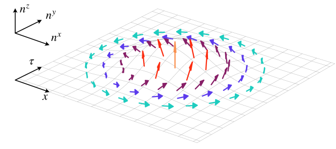
Figure 2: Meron configuration of staggered moment, $\bm{n}(x_{j})=(-1)^{j}\bm{S}_{j}$, with skyrmion number $+1/2$.

Here, we summarize the results obtained from the O(3) NL$\sigma$M approach. We give technical details in Appendix. B. The $S\in\mathbb{Z}+1/2$ cases fall into the $S=1/2$ case (3), where the staggered magnetic field induces the edge magnetization $\mathcal{P}=\pm 1/4$. With $h_{s}=0$, the half-odd-spin-$S$ HAFM chain has either the gapless ground state or doubly degenerate gapped ground state. The sine-Gordon theory as the dual theory of the O(3) NL$\sigma$M explains this impossibility of the unique and gapped ground state under the translation and spin-rotation symmetries. This argument is consistent with the LSM theorem on the spin-$S$ HAFM chain Lieb et al. (1961). The staggered magnetic field violates the one-site translation symmetry and makes the ground state unique and gapped.

The $S\in\mathbb{Z}$ cases are described by the sine-Gordon theory (33) with $g_{c}\propto-\cos(\pi S)$. The edge magnetization $\mathcal{P}=\pm 1/2\mod 1$ emerges only when $S\in 2\mathbb{Z}+1$ [Eq. (123)]. By contrast, $\mathcal{P}=0\mod 1$ follows from $\bar{\phi}=0\mod\pi$ for $S\in 2\mathbb{Z}$. This even-odd feature of the integer-spin-$S$ chain is consistent with the topological triviality (nontriviality) of the even-$S$ (odd-$S$) Haldane phase Pollmann et al. (2012); Tonegawa et al. (2011).

II.4 Symmetry protection of quantization

The quantization of the edge magnetization is protected by symmetries. Typical interactions that ruin the quantization are U(1)-breaking interactions such as $J_{x}\sum_{j=1}^{L}S_{j}^{x}S_{j+1}^{x}$. We can express this interaction in terms of the sine-Gordon theory as $\propto J_{x}\int_{0}^{L}dx\,\cos(2\theta)$, where $\theta$ is a canonical conjugate of $\phi$ Giamarchi (2004) that satisfies a commutation relation,

$$[\phi(x),\theta(y)]=i\pi\Theta_{\rm step}(x-y),$$ (40)

where $\Theta_{\rm step}(z)$ is the Heaviside step function,

$$\Theta_{\rm step}(z)=\left\{\begin{array}[]{ccc}1&&(z>0)\\[4.0pt] \frac{1}{2}&&(z=0)\\[4.0pt] 0&&(z<0)\end{array}.\right.$$ (44)

Equation (40) indicates that $\phi$ and $\theta$ are not locked at the same time.

Our “semiclassical bosonization” formula of the spin derived from the spin chain through the O(3) NL$\sigma$M (Appendix B.3.2) leads to $(-1)^{j}S_{j}^{+}\approx e^{i\theta}$ for the spin-$S$ chain just like the conventional one Giamarchi (2004). The global U(1) spin-rotation symmetry excludes $\cos(n\theta)$ and $\sin(n\theta)$ with $n\in\mathbb{Z}$ from the Hamiltonian.

Fixing the locking position $\bar{\phi}$ is also necessary to protect the quantization. If the effective Hamiltonian (3) for the spin-$1/2$ chain admits an interaction $g_{c}\cos(2\phi)$, the Hamiltonian is modified to

$$\mathcal{H}_{s}=\int_{0}^{L}dx\biggl{[}\frac{v}{2\pi K}(\partial_{\mu}\phi)^{2}+\sqrt{{g_{s}}^{2}+{g_{c}}^{2}}\sin(2\phi+A)\biggr{]},$$ (45)

with $A=\tan^{-1}(g_{c}/g_{s})$. The locking position gets shifted in accordance with the shifted potential $\sqrt{{g_{s}}^{2}+{g_{c}}^{2}}\sin(2\phi+A)$. The bulk polarization $\mathcal{P}$ gradually changes with $A$ Shindou (2005). Hence, we must forbid $\cos(2\phi)$ from entering into the spin-$1/2$ Hamiltonian (3) to keep $\mathcal{P}$ quantized. Likewise, we must forbid $\sin(2\phi)$ from the spin-1 Hamiltonian (33).

An inversion symmetry fixes the locking position of $\phi$. For the spin-1/2 chain, the site-centered inversion $\mathcal{I}_{s}:\,\bm{S}_{j}\to\bm{S}_{L-j}$ acts on $\phi$ as $\mathcal{I}_{s}:\,\phi(x)\to-\phi(L-x)+\pi/2$. This operation on $\phi$ is deduced from behaviors of the staggered magnetization $(-1)^{j}S_{j}^{z}\sim\sin(2\phi)$ and the dimerization $(-1)^{j}\bm{S}_{j}\cdot\bm{S}_{j+1}\sim\cos(2\phi)$. The site-centered inversion keeps the former invariant but changes the sign of the latter. The $\mathcal{I}_{s}$ symmetry thus excludes $\cos(2\phi)$ from the spin-1/2 chain (3). For the spin-1 chain, $\mathcal{I}_{s}$ instead acts on $\phi=\phi_{1}+\phi_{2}$ so that $\mathcal{I}_{s}:\,\phi(x)\to-\phi(L-x)+\pi$ because both $\phi_{1}$ and $\phi_{2}$ admit the $\pi/2$ shift under $\mathcal{I}_{s}$. The $\mathcal{I}_{s}$ symmetry thus excludes $\sin(2\phi)$ from the spin-1 chain (33). Based on our semiclassical bosonization formulas for the spin-$S$ HAFM chains, we reach the same conclusion that the U(1) spin-rotation and the $\mathcal{I}_{s}$ inversion symmetries protect the quantization of the edge magnetizations in the spin-$S$ HAFM chains.

The symmetry-protected edge magnetization gives an interesting characterization of quantum phases in one-dimensional quantum spin systems. Here, we point out that the edge-magnetization-based characterization of quantum phases is related to the concept of symmetry-protected trivial (SPt) phases Fuji et al. (2015). Though the precise relation between these two concepts is not clear yet, they are related indeed. According to Ref. Fuji et al. (2015), the induced Néel state $\ket{N}=\bigotimes_{j}\ket{S_{j}^{z}=(-1)^{j}}$ in a spin-$1$ chain is an SPt phase but the large-$D$ state $\ket{D}=\bigotimes_{j}\ket{S_{j}^{z}=0}$ is not. The former has $\mathcal{P}=1/2\mod 1$ and the latter has $\mathcal{P}=0\mod 1$, since $\braket{N}{U}{N}=-1$ and $\braket{D}{U}{D}=1$. Note that the spin-$1/2$ chain (1) has $\ket{N}$ as its ground state in the $h_{s}\to+\infty$ limit. We will summarize affinities and differences of our characterization of quantum phases with the odd-spn Haldane phase and the SPt phase later in Table. 1.

III Edge magnetization on magnetization plateau

The edge-magnetization-based characterization of quantum phases also works when the net magnetization is nonzero, $\sum_{\bm{r}}\braket{S_{\bm{r}}^{z}}\not=0$. Generally, the uniform magnetic field favors spatially nonuniform $\phi$ accompanied by gapless spin excitations [see Eq. (5)]. The uniform magnetic field $h_{u}$ indeed reduces the Haldane gap of the spin-1 chain and induces the quantum phase transition into a TL-liquid phase Giamarchi (2004); Schulz (1980); Chitra and Giamarchi (1997). However, the uniform magnetic field can also induce a quantum phase transition from the TL liquid phase into a spin gap phase. An increase of the uniform magnetic field can yield a spin gap state with a commensurate magnetization density, called a magnetization plateau Oshikawa et al. (1997). Magnetization plateaus are supposed to appear when $N_{0}(S-m)$ is a rational number Oshikawa et al. (1997), where $N_{0}$ is the number of spins per unit cell and $m$ is the magnetization per site.

III.1 Spin-1/2 ladder

Figure 3 shows numerical results about a spin-$1/2$ ladder that exhibits a magnetization plateau. Its Hamiltonian is given by,

$$\mathcal{H}_{\mathrm{ladder}} =J_{\parallel}\sum_{j=1}^{L-1}\sum_{n=1,2}\bm{S}_{j,n}\cdot\bm{S}_{j+1,n}-h_{u}\sum_{j=1}^{L}\sum_{n=1,2}S_{j,n}^{z}$$

$$\quad+\sum_{j=1}^{L}[J_{\perp}+(-1)^{j}J_{s}]\bm{S}_{j,1}\cdot\bm{S}_{j,2},$$ (46)

with $J_{\perp}\gg J_{\parallel}>0$, $J_{\perp}\gg J_{s}>0$, and $h_{s}>0$. The first term denotes the intra-chain HAFM interaction, the second term is the uniform Zeeman field, and the others are the uniform ($J_{\perp}$) and the staggered ($J_{s}$) rung interactions. All the numerical data in this paper are obtained from density-matrix renormalization group calculations with the OBC Fishman et al. (2020), where the bond dimension $100-1000$ and the truncation error $10^{-8}$ at largest are kept. While the spin ladder with $J_{s}=0$ does not exhibit the magnetization plateau, the staggered rung interaction, $J_{s}\sum_{j=1}^{L}(-1)^{j}\bm{S}_{j,1}\cdot\bm{S}_{j,2}$, induces the magnetization plateau with $M/M_{s}=1/2$, where $M_{s}$ is the saturated value of the magnetization (the inset of Fig. 3) Tonegawa et al. (1998).

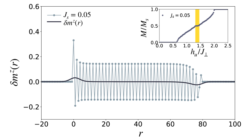
Figure 3: Site $r$ dependence of the “charge” $C_{r}$ of Eq. (50) with $N=2$ (filled balls) and $\delta m^{z}(r)$. The edge magnetizations on the left and right edges are quantized as $\pm 0.25000$. We used parameters $J_{\perp}=1$, $J_{\parallel}=0.5$, $J_{s}=0.05$, $h_{u}=1.4$, and $2L=160$. (inset) Magnetization curve. The shaded area highlights the $1/2$ magnetization plateau.

III.2 Pseudospin picture

The ground state of the model (46) on the $1/2$ plateau has an intuitive pseudospin picture Giamarchi (2004). For $J_{\parallel}=0$, the spin ladder (46) is fractured into a set of isolated antiferromagnetic dimers. Each dimer is described by a two-spin model

$$\mathcal{H}_{\text{dimer}}=J_{\perp}\bm{S}_{1}\cdot\bm{S}_{2}-h_{u}(S_{1}^{z}+S_{2}^{z}).$$ (47)

If $h_{u}=0$, the ground state of the model (47) is the singlet state, $\ket{s}=(\ket{\frac{1}{2},\,-\frac{1}{2}}-\ket{-\frac{1}{2},\,\frac{1}{2}})/\sqrt{2}$, where $\ket{S_{1}^{z},S_{2}^{z}}$ is the simultaneous eigenstate of $S_{n}^{z}$ for $n=1,2$. The dimer has triply degenerate spin-1 excited states, $\ket{t_{\sigma}}$ with $\sigma=1,0,-1$. The uniform magnetic field $h_{u}$ lifts the triple degeneracy and eventually makes $\ket{s}$ and $\ket{t_{1}}=\ket{\frac{1}{2},\,\frac{1}{2}}$ nearly degenerate, where we may discard the other high-energy excited states and regard $\ket{s}$ and $\ket{t_{1}}$ as the “down” and ”up” states of an $S=1/2$ pseudospin $\bm{T}_{j}$ Giamarchi and Tsvelik (1999); Bouillot et al. (2011).

We can regard the spin ladder (46) as a weakly coupled dimers for $J_{\parallel}/J_{\perp}\ll 1$ and, accordingly, as a pseudospin-$1/2$ chain. The perturbative expansion about $J_{\parallel}/J_{\perp}$ maps the spin-$1/2$ ladder (46) into the single pseudospin-$1/2$ XXZ chain with a staggered magnetic field,

$$\mathcal{H}_{\mathrm{ladder}} \approx J_{\parallel}\sum_{j=1}^{L}(T_{j}^{x}T_{j+1}^{x}+T_{j}^{y}T_{j+1}^{y}+\tfrac{1}{2}T_{j}^{z}T_{j+1}^{z})$$

$$\qquad-\sum_{j=1}^{L}(h_{\mathrm{eff}}-(-1)^{j}J_{s})T_{j}^{z},$$ (48)

with $h_{\rm eff}=h_{u}-J_{\perp}-\frac{J_{\parallel}}{2}$. The effective uniform magnetic field vanishes, $h_{\mathrm{eff}}=0$, for $M/M_{s}=1/2$ if $J_{s}=0$ Bouillot et al. (2011). Nonzero $J_{s}$ opens the spin gap around $h_{\rm eff}\approx 0$. In other words, the ground state is on the $1/2$ magnetization plateau around $h_{\rm eff}\approx 0$ for $J_{s}\not=0$. Similarly to the authentic spin-1/2 chain, the edge magnetization $\pm 1/4$ will appear in the pseudospin-$1/2$ chain (Fig. 3).

III.3 General definition of edge magnetization on magnetization plateaus

Let us formulate the edge magnetization on the magnetization plateau based on a nonlocal operator $U$. A naive definition of the operator $U$ in the spin ladder will be

$$U_{\rm naive}=\exp\biggl{(}i\frac{2\pi}{L}\sum_{j=1}^{L}j\sum_{n=1}^{N_{0}}S_{j,n}^{z}\biggr{)},$$ (49)

where $S_{j,n}^{z}$ is the $z$ component of a spin $\bm{S}_{j,n}$ in the unit cell located at the position $j$. The unit cell contains $N_{0}=4$ spins for $J_{s}\not=0$. The operator $U_{\rm naive}$ of Eq. (49) seems ambiguous on the magnetization plateau because, if we regard $S_{j}^{z}$ as a charge, the charge neutrality condition (2) is violated on the magnetization plateau. Suppose that the magnetization per site $m$ is fractional, namely $m=p/q$ with coprime positive integers $p$ and $q$. The naive operator (49) gives $\braket{U_{\rm naive}}=\exp(2\pi mi(L+1))$. Since $m$ is fractional, $U_{\rm naive}$ formally leads to $\mathcal{P}\not=0$. However, this $\mathcal{P}\not=0$ cannot be deemed the edge magnetization because it originates from the bulk uniform magnetization. To make the edge magnetization well defined on the nonzero magnetization plateau, we need to define an appropriate charge that satisfies a charge neutrality condition. In general one-dimensional quantum spin systems on magnetization plateaus, we can adopt

$$U=\exp\biggl{(}i\frac{2\pi}{L}\sum_{j=1}^{L}jC_{j}\biggr{)},\quad C_{j}=\sum_{n=1}^{N}(S_{j,n}^{z}-m),$$ (50)

where $C_{j}$ is the charge density for $m\not=0$. The naive choice of $N$ will be $N=N_{0}$, the number of spins per unit cell. However, $N$ can be smaller than $N_{0}$. Recall that we took $N=1$ for the spin-$1/2$ chain (1) despite $N_{0}=2$. We take $N=2$ for the spin ladder (46) even for $J_{s}\not=0$, where $N_{0}=4$. The magnetization plateau satisfies the charge neutrality,

$$\sum_{j=1}^{L}\braket{C_{j}}=0.$$ (51)

We modify the definition of the edge magnetizations in accordance with the definition of the charge $C_{j}$.

$$M_{\mathrm{left}}^{z} =\int_{-\infty}^{\frac{L+1}{2}}dr\,\delta m^{z}(r),\quad M_{\mathrm{right}}^{z}=\int_{\frac{L+1}{2}}^{\infty}dr\,\delta m^{z}(r),$$ (52)

$$\delta m^{z}(r) =\sum_{r^{\prime}=1}^{L}g(r-r^{\prime})\braket{C_{r^{\prime}}}.$$ (53)

For the spin ladder (46) on the $1/2$ plateau, Eq. (50) gives

$$U=\exp\biggl{(}i\frac{2\pi}{L}\sum_{j=1}^{L}jT_{j}^{z}\biggr{)},$$ (54)

dealing with the pseudospin-$1/2$ chain in analogy with the authentic spin-$1/2$ chain. Figure 3 shows the spatial distribution of $\braket{C_{r}}$ and $\delta m^{z}(r)$ for the spin-$1/2$ ladder (46) on the $1/2$ magnetization plateau . The edge magnetizations (52) exhibit the excellent quantization $M_{\mathrm{left}}^{z}=-M_{\mathrm{right}}^{z}=0.25000$ despite the small $J_{s}\ll J_{\perp}$. We used the Gaussian $g(r)$ with $\lambda=3$. The Lorentzian $g(r)=(\varepsilon/\pi)/(r^{2}+\varepsilon^{2})$ also exhibits the edge magnetization but its quantization is less accurate. We also confirmed that the quantization accuracy is insensitive to the value of $\lambda$.

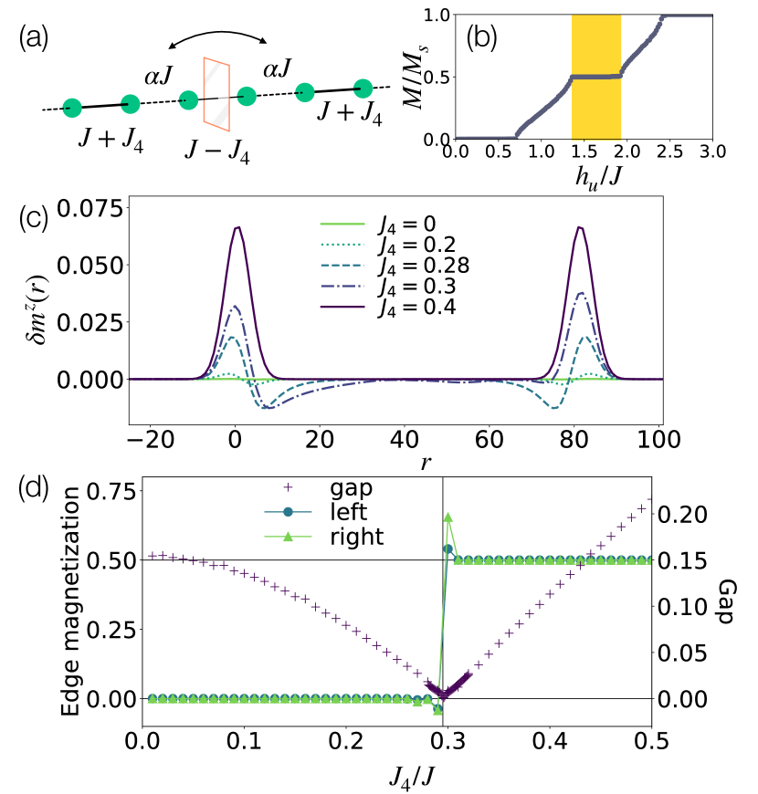
Figure 4: (a) Spin-1 chain (55) with bond-inversion center. (b) Magnetization curve for $J_{4}=0$. (c) Site $r$ dependence of $\delta m^{z}(r)$ (d) $J_{4}$ dependence of lowest-energy excitation gap ($+$ markers) and edge magnetizations (53) (circles and triangles). The edge magnetizations are quantized as $M_{\mathrm{left}}^{z}=M_{\mathrm{right}}^{z}=0.499999999$ for $J_{4}>J_{4c}\approx 0.295$. We used parameters $J=1$, $\alpha=0.2$, $h_{u}=1.5$. The system size is $L=162$ for (b,c) and $242$ for (d).

IV Charge jump at quantum critical point

The spin-$1/2$ ladder (46) is the prototypical model that exhibits the quantized edge magnetizations on the nonzero magnetization plateau. In what follows, we consider a thought-provoking model whose edge magnetization jumps from zero to a nonzero value at a quantum critical point on the plateau.

IV.1 Four-site periodic spin-1 chain and its pseudospin picture

The model is a spin-1 HAFM chain with a four-site periodic structure [Fig. 4 (a)],

$$\mathcal{H}_{4} =J\sum_{j=1}^{\frac{L-2}{2}}(\bm{S}_{2j-1}\cdot\bm{S}_{2j}+\alpha\bm{S}_{2j}\cdot\bm{S}_{2j+1})$$

$$\qquad+J_{4}\sum_{j=1}^{\frac{L}{2}}(-1)^{j}\bm{S}_{2j-1}\cdot\bm{S}_{2j}-h_{u}\sum_{j}S_{j}^{z},$$ (55)

where $\bm{S}_{j}$ is the spin-1 operator at the $j$th site. $0\leq\alpha\leq 1$ and $0\leq J_{4}<J$. The parameter $\alpha$ denotes the bond alternation for $\alpha\not=1$. The $J_{4}$ interaction is the four-site periodic exchange interaction. We can label $\bm{S}_{2j-1}=\bm{S}_{r,1}$ and $\bm{S}_{2j}=\bm{S}_{r,2}$ for $r=1,2,\cdots,L/2$. Here, we define the charge (50) as

$$C_{r}=\sum_{n=1}^{2}(S_{r,n}^{z}-m).$$ (56)

The bond-alternating chain (55) shows magnetization plateaus [Fig. 4 (b)]. The $1/2$ plateau for $J_{4}=0$ was experimentally observed Narumi et al. (2004). We can see this $1/2$ plateau as a forced ferromagnetic phase of another $S=1/2$ pseudospin, $\tilde{\bm{T}}_{j}$. For $\alpha=0$, the model (55) is reduced to isolated spin-1 dimers. Each dimer is described by the Hamiltonian (47). This time, the spin quantum number of $\bm{S}_{1}$ and $\bm{S}_{2}$ are $S=1$. For $h_{u}=0$, each dimer has the spin-0 singlet ground state, $\ket{s}=(\ket{1,-1}+\ket{-1,1}-\ket{0,0})/\sqrt{3}$. The magnetic field reduces the excitaton energy of a spin-1 state $\ket{t_{1}}=(\ket{1,0}-\ket{0,1})/\sqrt{2}$ and makes $\ket{s}$ and $\ket{t_{1}}$ degenerate at $M/M_{s}=1/4$. Regarding $\ket{s}$ and $\ket{t_{1}}$ as the “down” and ”up” state of the $S=1/2$ pseudospin $\tilde{\bm{T}}_{j}$, we can rewrite the Hamiltonian (55) as

$$\mathcal{H}_{4} \approx\frac{J\alpha}{3}\sum_{j}(\tilde{T}_{j}^{x}\tilde{T}_{j+1}^{x}+\tilde{T}_{j}^{y}\tilde{T}_{j+1}^{y}+\tfrac{3}{4}\tilde{T}_{j}^{z}\tilde{T}_{j+1}^{z})$$

$$\qquad-\sum_{j}(h^{\prime}_{\mathrm{eff}}-(-1)^{j}J_{4})\tilde{T}_{j}^{z}$$ (57)

within the first-order approximation about $\alpha$ Okamoto et al. (2001). The $J_{4}$ interaction turns into the staggered magnetic field, which induces the $1/4$ magnetization plateau around $h^{\prime}_{\mathrm{eff}}=0$. As $h^{\prime}_{\mathrm{eff}}$ is increased from zero, the pseudospin chain eventually reaches the forced ferromagnetic phase of the pseudospin, that is, the $1/2$ magnetization plateau with $\braket{S_{2j-1}^{z}}=\braket{S_{2j}^{z}}=(1+2\braket{\tilde{T}_{j}^{z}})/4=1/2$. The $1/2$ magnetization plateau thus exists even for $J_{4}=0$ Totsuka (1997).

To understand the magnetization process for $M/M_{s}>1/2$, we need to go beyond this pseudospin approximation. For $M/M_{s}>1/2$, a spin-2 state $\ket{q_{2}}=\ket{1,1}$ of the spin-1 dimer enters into the ground state. The inter-dimer interactions make $\ket{q_{2}}$ dispersive. The magnetization process for $1/2<M/M_{s}\leq 1$ corresponds to a process that increases a population of $\ket{q_{2}}$ in the ground state.

IV.2 Quantum phase transition on 1/2 magnetization plateau

The effective staggered magnetic field $J_{4}(-1)^{j}\tilde{T}_{j}^{z}$ would seem to drag the ground state away from the $1/2$ plateau since the forced Néel state $\bigotimes_{j=1}^{L/2}\ket{\tilde{T}_{j}^{z}=(-1)^{j+1}/2}$ in accordance with the effective staggered-field interaction has $M/M_{s}=1/4$. However, the $J_{4}$ interaction induces a quantum phase transition without dragging the ground state away from the $1/2$ plateau. Figure 4 (c) shows the $J_{4}$ dependence of $M_{\mathrm{left}}^{z}$ and $M_{\mathrm{right}}^{z}$. We chose $L=162$ to keep the bond-centered inversion symmetry, $\mathcal{I}_{b}:\,\bm{S}_{j}\to\bm{S}_{L+1-j}$ under the OBC. The model (55) is $\mathcal{I}_{b}$-invariant only when $L=2\mod 4$ . The U(1) spin-rotation and $\mathcal{I}_{b}$ symmetries protect the quantization of the edge magnetization, as we see later. The $\mathcal{I}_{s}$ cannot protect the quantization of the edge magnetization. The spatial dependence $\delta m^{z}(r)$ gradually changes as $J_{4}$ is increased [Fig. 4 (c)]. Nevertheless, the edge magnetizations shows a jump from zero to $1/2$ at $J_{4}=J_{4c}\approx 0.295J$ [Fig. 4 (d)] since the above symmetries forbid the continuous change [Eq. (215)].

An effective field theory gives a straightforward way to understand the charge jump. It was previously shown that the effective field theory on the magnetization plateau becomes the sine-Gordon theory for $S-m\in\mathbb{Z}$ Tanaka et al. (2009); Takayoshi et al. (2015). This sine-Gordon theory itself is inapplicable to the current situation of our interest with $S-m=1/2$. However, we can modify the argument of Refs. Tanaka et al. (2009); Takayoshi et al. (2015) to fit into our situation (Appendix C.3.3). We can resolve the issue of the fractional $S-m$ by properly counting topological sectors. The previously considered case with $S-m\in\mathbb{Z}$ involves the single topological sector. Our case with $S-m\in\mathbb{Z}+1/2$ involves two topological sectors. This topological difference governs the behavior of the effective field theory.

Let us first discuss the effective field theory in the bulk by imposing the periodic boundary condition, $\bm{S}_{j+L}=\bm{S}_{j}$, on the spin chain (55). When $\alpha-1=J_{4}=0$, the spin chain (55) is the uniform spin-1 HAFM chain. When $S-m=1/2$, the spin-1 chain is described by an effective field theory with the following Hamiltonian [see Eq. (200)]:

$$\mathcal{H}_{\rm eff} \approx\frac{v}{2\pi K}\int dx\,(\partial_{\mu}\phi)^{2}$$

$$\qquad-2\zeta^{2}\cos[2\pi(S-m)]\int dx\,\cos(4\phi),$$ (58)

where $\zeta$ is a fugacity of a vortex Tanaka et al. (2009); Takayoshi et al. (2015). When the $\cos(4\phi)$ interaction is relevant, the spin-1 chain shows the magnetization plateau by spontaneously breaking the one-site translation symmetry, $T_{1}:\bm{S}_{j}\to\bm{S}_{j+1}$. When the $\cos(4\phi)$ interaction is irrelevant, the spin-1 chain has the gapless TL-liquid ground state for $S-m=1/2$. While it is hard to judge which is the case only from the effective field theory, we know numerically that the gapless scenario is the case Takahashi and Sakai (1991). Hence, we may drop the $\cos(4\phi)$ term from the Hamiltonian (58).

The $T_{1}$ symmetry is translated into Eq. (186), namely,

$$\phi(x)\to\phi(x)+\frac{\pi}{2},$$ (59)

$$\theta(x)\to\theta(x)+\pi,$$ (60)

in the field theory language, which excludes $\cos(2\phi)$ and $\sin(2\phi)$ from the Hamiltonian. The absence of $\cos(2\phi)$ and $\sin(2\phi)$ is due to the destructive interference between the two topological sectors. The bond alternation $\alpha\not=1$ and the $J_{4}$ interaction break the $T_{1}$ symmetry and unbalance the interference between the topological sectors. The model (55) on the $1/2$ plateau is mapped to the sine-Gordon theory,

$$\mathcal{H}_{4} =\int_{0}^{L}dx\biggl{[}\frac{v}{2\pi K}(\partial_{\mu}\phi)^{2}+(g_{2}(J_{4})-g_{2c})\cos(2\phi)\biggr{]},$$ (61)

with $g_{2}(J_{4})\propto(J_{4})^{2}/J$ and $g_{2c}\propto(1-\alpha)J$. The $J_{4}$ interaction of Eq. (55) is taken into account perturbatively. The $J_{4}$ interaction gives rise to $\cos(2\phi)$ in a second-order perturbation process (Appendix D) because the $J_{4}$ interaction has the four-site periodicity. The cosine interaction $\cos(2\phi)$ is the most relevant interaction with the two-site periodicity in accordance with the antiferromagnetic fluctuations. The second-order perturbation expansion is required to produce the two-site periodic interaction from the four-site one. Note that $\sin(2\phi)$ is still forbidden because of the $\mathcal{I}_{b}$ symmetry, $\phi(x)\to-\phi(L-x)\mod 2\pi$ [Eq. (195)].

Next, we impose the OBC on the spin chain (55). The $T_{1}$ symmetry is lost, but the $\mathcal{I}_{b}$ symmetry survives in the OBC. The effective Hamiltonian (61) thus holds with the OBC as well as the periodic one. When $J_{4}=0$, the sine-Gordon theory (61) with $g_{2c}>0$ locks $\bar{\phi}=0$ (i.e. $\mathcal{P}=0$). $J_{4}\not=0$ makes $g_{2}(J_{4})>0$. An increase of $J_{4}>0$ drags the system into the quantum critical point $J_{4}=J_{4c}$, where $g_{2}(J_{4})=g_{2c}$ holds. For $J_{4}>J_{4c}$, the sine-Gordon theory (61) with $g_{2}(J_{4})-g_{2c}<0$ locks $\bar{\phi}=\pi/2$ (i.e. $\mathcal{P}=1/2$).

IV.3 Topological transition on magnetization plateau

Figure 5: (a) $J_{4}$ dependence of lowest-energy excitation gap for $h_{u}/J=1.5$, $\alpha=0.2$, and $L=122$ (circles) and $L=242$ ($+$ markers). (b) Numerically calculated entanglement entropy for $h_{u}/J=1.5$, $\alpha=0.2$, and $L=242$ (circles) and the fitting function (62) with $(a_{s},c)=(0.52,0.94)$. The central charge $c\approx 1$ is consistent with the sine-Gordon theory (61).

Numerical results show that the quantum phase transition at $J_{4}=J_{4c}$ is likely to be a quantum critical one with the gap closing [Fig. 4 (d), Fig. 5 (a)]. In the quantum critical regime, the entanglement entropy shows the logarithmic scaling Calabrese and Cardy (2004) [Fig. 5 (b)],

$$\mathcal{S}_{\rm EE}(x) =a_{s}+\frac{c}{6}\ln\biggl{[}\frac{L}{\pi}\sin\biggl{(}\frac{\pi x}{L}\biggr{)}\biggr{]},$$ (62)

with a constant $a_{s}$ and the central charge $c$. The central charge characterizes the conformal field theory that corresponds to the quantum critical point. The numerical estimation $c\approx 0.94$ is consistent with $c=1$ of the effective field theory (61) with $g_{2}(J_{4})=g_{2c}$. The gap is thus highly likely to be closed at the transition point $g_{2}(J_{4})=g_{2c}$. Even if the phase transition should be weakly first-order, our field theory (61) still holds by taking into account a less relevant interaction, $\cos(4\phi)$, which is dropped in Eq. (61) (see Eq. (214)). If the first-order transition scenario comes true, the $J_{4}$ interaction must affect the scaling dimension of the $\cos(4\phi)$ interaction to make it relevant.

Despite the ground state’s quantum critical behavior, the edge magnetization shows the abrupt change, reflecting its topological nature. The quantization of the edge magnetization is an exact property of the spin chain (55). The $\mathcal{I}_{b}$ symmetry of the Hamiltonian imposes that

$$\braket{U}=\braket{\mathcal{I}_{b}U\mathcal{I}_{b}^{-1}}=\braket{U^{\dagger}}.$$ (63)

It follows that $\operatorname{Im}\ln\braket{U}=-\operatorname{Im}\ln\braket{U}\mod 2\pi$. Namely, the $\mathcal{I}_{b}$ imposes

$$\mathcal{P} =0,\>\text{ or }\>\frac{1}{2}\mod 1.$$ (64)

This is consistent with the numerical results. $\mathcal{P}=0$ holds for $J_{4}<J_{4c}$ and $\mathcal{P}=1/2$ for $J_{4}>J_{4c}$.

Our quantum field theory (61) also supports the fact that the U(1) spin-rotation and the $\mathcal{I}_{b}$ symmetries protect the quantization of the edge magnetization. According to Eqs. (195), the $\mathcal{I}_{b}$ symmetry forbids $\sin(n\phi)$ with $n\in\mathbb{Z}$ from entering into the effective Hamiltonian. Besides, the U(1) spin-rotation symmetry forbids $\cos(n\theta)$ and $\sin(n\theta)$. Therefore, the quantization of the edge magnetization of the spin-1 chain (55) on the $1/2$ plateau is protected by the U(1) spin-rotation and the $\mathcal{I}_{b}$ symmetry.

Precisely speaking, the ground state for $J_{4}>J_{4c}$ violates the charge neutrality condition (51) because of $M_{\mathrm{left}}^{z}=M_{\mathrm{right}}^{z}=1/2$ [Figs. 4 (c), (d)]. $\sum_{j=1}^{L}\braket{C_{j}}=1$ holds for $J_{4}>J_{4c}$ whereas $\sum_{j=1}^{L}\braket{C_{j}}=0$ for $J_{4}<J_{4c}$. Nevertheless, the ground state remains on the $1/2$ plateau for $J_{4}>J_{4c}$ in the thermodynamic limit since $\frac{M}{M_{s}}=\frac{1}{2}(1+\frac{1}{L})\to\frac{1}{2}$.

Thus far, we have developed the effective field theory to understand the topological quantum phase transition of the spin-1 chain (55) on the $1/2$ magnetization plateau. We employed the effective field theory approach because the pseudospin approximation seemed powerless. Still, the weakly-coupled dimer picture at $|\alpha|\ll 1$ gives us some intuition to understand the abrupt charge jump at $J_{4}=J_{4c}$. When $J_{4}=\alpha=0$, the ground state is the product state of $\ket{t_{1}}$. The $J_{4}$ interaction weakens antiferromagnetic intradimer coupling, $J-J_{4}$, and invites the spin-2 state, $\ket{q_{2}}$, to join the low-energy physics. Let us compare the energies of two product states $\ket{t_{1}}_{1}\ket{t_{1}}_{2}\cdots\ket{t_{1}}_{L/2}$ and $\ket{t_{1}}_{1}\ket{t_{1}}_{2}\cdots\ket{q_{2}}_{r_{1}}\cdots\ket{t_{1}}_{L/2}$, where we replace $\ket{t_{1}}_{r_{1}}$ by $\ket{q_{2}}_{r_{1}}$ for one dimer at $r_{1}$. Let $E$ and $E^{\prime}$ be eigenenergies of the former and latter states for $\alpha=0$. The latter becomes the ground state when their energy difference $\Delta E:=E^{\prime}-E$,

$$\Delta E =2(J-J_{4})-h_{u}$$ (65)

becomes negative, that is, when $J_{4}>J_{4d}$ with

$$J_{4d} =\frac{2J-h_{u}}{2}.$$ (66)

For $\alpha=0$, the first-order transition occurs at $J_{4}=J_{4d}$ because every $\ket{t_{1}}$ is replaced by $\ket{q_{2}}$ as $J_{4}$ passes $J_{4d}$. For $\alpha\not=0$, the inter-dimer exchange interaction minimizes the number of $\ket{q_{2}}$ to minimize the energy cost due to the antiferromagnetic $J\alpha$ interaction. The number of $\ket{q_{2}}$ is zero for $J_{4}<J_{4d}$ and will be one for $J_{4}>J_{4d}$. For the parameter set of Fig. 4, we obtain $J_{4d}=0.25$, close enough to $J_{4c}\approx 0.295$ where the topological transition actually occurs. When one of $\ket{t_{1}}$ is replaced by the spin-2 $\ket{q_{2}}$, the spin-$2$ object will be delocalized to minimize the energy cost arising from the antiferromagnetic exchange interactions. If $\ket{q_{2}}$ carrying the charge one is shunted off to the edges, it is fractionalized to two $1/2$ charges to keep the exact $\mathcal{I}_{b}$ symmetry. We thus end up with the edge magnetizations $M_{\rm left}^{z}=M_{\rm right}^{z}=1/2$.

V Edge magnetization of ferrimagnets

The edge magnetizations hitherto considered are triggered by spatially nonuniform interactions. Even if the edge magnetization has a topological origin such as the spin-1 Haldane phase of the uniform spin-1 HAFM chain, the staggered magnetic field is necessary to make the edge magnetization visible by lifting the degeneracy of the edge state. In this sense, we thus far needed spatially nonuniform interactions to trigger the edge magnetization by breaking the inversion symmetry that protects the edge-state degeneracy.

Here, we discuss a contrasting case that the uniform magnetic field triggers the edge magnetization by lifting the ground-state degeneracy. We deal with a spin-$1/2$ HAFM model on a union-jack strip [Fig. 6 (a)] Shimokawa and Nakano (2013); Furuya and Giamarchi (2014),

$$\mathcal{H}_{\rm UJ} =J_{1}\sum_{j=1}^{L}\sum_{n=1}^{3}\bm{S}_{j,n}\cdot\bm{S}_{j+1,n}+J_{1}\sum_{j=1}^{L}\bm{S}_{j,2}\cdot(\bm{S}_{j,1}+\bm{S}_{j,3})$$

$$+J_{2}\sum_{j=2}^{L-1}\bm{S}_{j,2}\cdot(\bm{S}_{j-1,1}+\bm{S}_{j-1,3}+\bm{S}_{j+1,1}+\bm{S}_{j+1,3}),$$ (67)

where $\bm{S}_{j,n}$ is the spin-$1/2$ operator. The first term denotes the intra-chain interaction, the second term denotes the rung interaction, and the last one denotes the inter-chain diagonal interactions.

For large enough $J_{2}/J_{1}>0$, this frustrated three-leg spin ladder exhibits a spontaneous magnetization plateau with $|M|/M_{s}=1/3$ by spontaneously breaking the SU(2) spin-rotation symmetry Shimokawa and Nakano (2013). The spontaneous ferromagnetic order is accompanied by an antiferromagnetic order thanks to the lattice structure. Namely, the ground state has the spontaneous long-range commensurate ferrimagnetic order. The ferrimagnetic order leads to $\mathcal{P}\not=0$, as we show below. However, similarly to the spin-1 Haldane phase, the edge magnetization is concealed by a $\mathbb{Z}_{2}$ symmetry, for example, a $\pi$ rotation symmetry $(S_{j,n}^{x},S_{j,n}^{y},S_{j,n}^{z})\to(S_{j,n}^{x},-S_{j,n}^{y},-S_{j,n}^{z})$ around the $x$ axis.

Figure 6: (a) Union-jack strip. (b) Site $r$ dependence of $\braket{C_{j}}$ and $\delta m^{z}(r)$ with $N=3$ and $m=1/6$. The edge magnetizations are quantized as $M_{\mathrm{right}}^{z}=-M_{\mathrm{left}}^{z}=0.5000000$. We used $J_{1}=1$, $J_{4}=4$, $h_{u}=0.1$, and $3L=240$.

Different from the spin-1 Haldane phase, an infinitesimal uniform magnetic field completely lifts the ground-state degeneracy by choosing one of the spontaneous ferrimagnetic states. In the presence of the weak uniform magnetic field, the effective field theory of the union-jack strip on the $1/3$ plateau has the following Hamiltonian (Appendix E),

$$\mathcal{H}_{\mathrm{UJ}} =\int_{0}^{L}dx\biggl{[}\frac{v}{2\pi K}(\partial_{\mu}\phi)^{2}+\zeta\cos(2\phi)\biggr{]}.$$ (68)

The $\phi$ field is related to the charge as $C_{j}=\sum_{n=1}^{3}S_{j,n}^{z}=\partial_{x}\phi/\pi$. The cosine interaction locks $\phi$ to $\bar{\phi}=\pm\pi/2$ and gives $\mathcal{P}=\mp 1/2$. Tracing the hitherto developed argument, we can confirm that the U(1) and $\mathcal{I}_{s}$ symmetries protect the quantization of the edge magnetization $\mathcal{P}=1/2$. Our $3L=240$-site calculation shows the fine quantization $M_{\mathrm{right}}^{z}=-M_{\mathrm{left}}^{z}=0.50000000$. Note that not $\mathcal{I}_{b}$ but $\mathcal{I}_{s}$ protects the quantization in contrast to the spin-1 chain (55) on the $1/2$ plateau. This symmetry difference ultimately comes from the difference in number of spin ladders’ legs .

In the absence of the uniform magnetic field, the magnetization plateau with $m=1/3$ and $m=-1/3$ are degenerate, where the edge magnetizations are concealed by the ground-state degeneracy. The uniform magnetic field chooses, for example, the $m=1/3$ state and makes the ground state unique and gapped. Then, nothing conceals the edge magnetization any longer [Fig. 6 (b)].

VI Conclusion and outlook

quantum phase	edge magnetization?	on plateau?
odd-spin Haldane (SPT)	no	yes Oshikawa et al. (1997); Takayoshi et al. (2014)
induced Néel (SPt)	yes	not found yet
large-$D$ (trivial)	no	yes Sakai and Takahashi (1998); Kitazawa and Okamoto (2000)
quantized $\mathcal{P}$	yes	yes

Table 1: Comparison of quantum phases with symmetry-protected quantized edge magnetization $\mathcal{P}$ (fifth row) with odd-spin Haldane phases (second row), an SPt phase (third row), and a trivial phase (fourth row). We numerically and field-theoretically found quantum phases accompanied by edge magnetizations on magnetization plateaus $m=0$ or $m\not=0$, which are referred to as ”quantized $\mathcal{P}$ in the table. The odd-spin Haldane phase, a symmetry-protected topological (SPT) phase, exhibit no edge magnetizations because a protecting symmetry forbids it. The quantized-$\mathcal{P}$ phase as well as the odd-spin Haldane phase are realized on a nonzero magnetization plateau Takayoshi et al. (2015). The SPt phase can exhibit the edge magnetization but is not found yet on nonzero magnetization plateaus.

We discussed the edge magnetization as the magnetic analog of the surface electric charge by using the low-energy effective field theory and the numerical density-matrix renormalization group method. Low-energy physics of one-dimensional quantum spin systems with or without the magnetization per site is described by the same effective field theory, the sine-Gordon theory.

The sine-Gordon theory is the strongly interacting field theory of the U(1) boson field $\phi$. We showed that the edge magnetization as the surface electric charge is the zero mode of $\phi$ [Eq. (13)]. The quantization of the zero mode is protected by the U(1) spin-rotation and inversion symmetries. The inversion symmetry can be either the site-centered or bond-centered one, depending on the carrier of the charge [Eq. (50)] and the number of spin chains.

We characterized quantum phases of one-dimensional quantum spin systems based on the edge magnetization and the symmetry protection of its quantization. We found some affinities and differences of this characterization with the odd-spin Haldane phase (a symmetry-protected topological phase) and the SPt phase as summarized in Table. 1. The edge magnetization turned out to give us an interesting viewpoint of the classification of quantum phases. Moreover, in principle, the edge magnetization is an observable quantity and will be relevant to experimental studies.

Our field-theoretical results on one-dimensional quantum spin systems will be useful as building blocks to construct magnetic analog of corner magnetizations in two- or three-dimensional quantum spin systems Watanabe et al. (2021) in the spirit of the coupled-wire construction Kane et al. (2002); Teo and Kane (2014); Meng et al. (2015); Lecheminant and Tsvelik (2017).

Appendix A Open boundary condition in spin chains

The open boundary condition (OBC) on the quantum spin-1/2 chain is formulated in a fermion language Eggert and Affleck (1992). The spin-1/2 operator $\bm{S}_{j}$ is written as Giamarchi (2004)

$$S_{j}^{z} =\psi_{j}^{\dagger}\psi_{j}-\frac{1}{2},$$ (69)

$$S_{j}^{+} =\psi_{j}^{\dagger}\exp\biggl{(}i\sum_{k=1}^{j-1}\psi_{k}^{\dagger}\psi_{k}\biggr{)},$$ (70)

where $\psi_{j}$ is an annihilation operator of a spinless fermion. The spinless fermion $\psi(x)=\psi_{j}/\sqrt{a_{0}}$ is split into right-moving $\psi_{R}(x)$ and left-moving $\psi_{L}(x)$ parts: $\psi(x)=e^{-ik_{F}x}\psi_{L}(x)+e^{ik_{F}x}\psi_{R}(x)$ with $x=ja_{0}$ and the Fermi wavenumber $k_{F}=\pi/2a_{0}$ Giamarchi (2004). We impose the OBC at $x=0$ on the spinless fermion by requiring the following conditions Eggert and Affleck (1992),

$$\psi(0)=\psi(L)=0.$$ (71)

Note that chiral fermion operaetors, $\psi_{L}$ and $\psi_{R}$ cancel each other so that Eq. (71) holds. This boundary condition is further translated into that for $\phi(x)$ and $\theta(x)$ via the following bosonization formula Giamarchi (2004),

$$\psi_{R}(x) \sim e^{-i(\theta-\phi)},\qquad\psi_{L}(x)\sim e^{-i(\theta+\phi)}.$$ (72)

Two boson fields $\phi(x)$ and $\theta(x)$ satisfy the commutation relation,

$$[\phi(x),\theta(y)]=i\pi\Theta_{\rm step}(y-x),$$ (73)

where $\Theta_{\rm step}(z)$ is the step function,

$$\Theta_{\rm step}(z) =\left\{\begin{array}[]{ccc}1&&(z>0)\\ 1/2&&(z=0)\\ 0&&(z<0)\end{array}\right..$$ (77)

This bosonization formula leads to, for instance, $(-1)^{j}S_{j}^{z}\approx a_{1}\sin(2\phi)+\cdots$ because $S_{j}^{z}=\psi_{j}^{\dagger}\psi_{j}-\frac{1}{2}$,

$$\psi^{\dagger}(x)\psi(x) =\psi_{R}^{\dagger}(x)\psi_{R}(x)+\psi_{L}^{\dagger}(x)\psi_{L}(x)$$

$$\quad+(-1)^{j}\bigl{[}\psi_{R}^{\dagger}(x)\psi_{L}(x)+\psi_{L}^{\dagger}(x)\psi_{R}(x)\bigr{]},$$ (78)

and

$$\psi_{R}^{\dagger}(x)\psi_{L}(x)+\psi_{L}^{\dagger}(x)\psi_{R}(x)$$

$$\sim e^{-2i\phi(x)+[\phi(x),\theta(x)]}+e^{2i\phi(x)-[\phi(x),\theta(x)]}$$

$$=2\sin(2\phi).$$ (79)

The boundary condition, $\psi(0)=0$, on the left edge leads to Eggert and Affleck (1992)

$$1-e^{2i\phi(0)}=0,$$ (80)

namely,

$$\phi(0) =0\mod\pi.$$ (81)

On the other edge, we obtain

$$1-e^{2ik_{F}L}e^{2i\phi(L)}=0.$$ (82)

Since $L/a_{0}$ must be an even integer to meet the charge-neutrality condition, we find

$$\phi(L)=0\mod\pi.$$ (83)

This boundary condition $\phi(0)=\phi(L)=0\mod\pi$ is consistent with the charge neutrality condition,

$$\sum_{j=1}^{L}S_{j}^{z}=\frac{1}{\pi}[\phi(L)-\phi(0)]=0.$$ (84)

The OBC on the spin chain is interpreted as the Dirichlet boundary condition on $\phi(x)$ at $x=0,\,L$. Equations (81) and (83) leads to

$$\partial_{t}\phi(x)\Bigr{|}_{x=0,L}=0.$$ (85)

The $\phi$’s canonical conjugate, $\theta$, then satisfies the Neumann boundary condition Furuya and Oshikawa (2012):

$$\partial_{x}\theta(x)\Bigr{|}_{x=0,L}=0.$$ (86)

Appendix B Semiclassical bosonization at zero magnetic fields

This section describes a derivation of the sine-Gordon theories for the spin-$S$ chain from the O(3) nonlinear sigma model (NL$\sigma$M). Here, we deal with zero-field cases.

B.1 Classical Hamiltonian of nonlinear sigma model

We start with the mapping of the spin operator $\bm{S}_{j}$ to slowly varying fields $\bm{n}(x_{j})$ and $\bm{L}(x_{j})$ Sachdev (2007):

$$\bm{S}_{j} =S\bm{\Omega}(x_{j}),$$ (87)

$$\bm{\Omega}(x_{j}) =(-1)^{j}\bm{n}(x_{j})\sqrt{1-\biggl{(}\frac{a_{0}\bm{L}(x_{j})}{S}\biggr{)}^{2}}+\frac{a_{0}}{S}\bm{L}(x_{j}),$$ (88)

where $S$ is the spin quantum number, $x_{j}=ja_{0}$ is the spatial coordinate, and $\bm{\Omega}(x_{j})$ is the three-component unit vector with $|\bm{\Omega}(x_{j})|^{2}=1$. Two quantum fields $\bm{n}(x)$ and $\bm{L}(x)$ satisfy $|\bm{n}(x)|^{2}=1$ and $\bm{n}(x)\cdot\bm{L}(x)=0$ for every $x$ so that $|\bm{\Omega}(x)|^{2}=1$. To respect the SU(2) commutation relation $[S_{j}^{a},S_{k}^{b}]=i\varepsilon^{abc}\delta_{j,k}S_{j}^{c}$, the following commutation relations are required Sachdev (2007).

$$[L^{a}(x),L^{b}(x)] =i\varepsilon^{abc}L^{c}(x)\delta(x-y),$$ (89)

$$[L^{a}(x),n^{b}(x)] =i\varepsilon^{abc}n^{c}(x)\delta(x-y),$$ (90)

$$[n^{a}(x),n^{b}(x)] =0,$$ (91)

where $\varepsilon^{abc}$ is the complete antisymmetric tensor with $\varepsilon^{xyz}=1$ and $\delta_{i,j}$ is the Kronecker’s delta.

Let us consider the partition function $Z$ of the spin-$S$ Heisenberg antiferromagnetic spin chain,

$$\mathcal{H}=J\sum_{j}\bm{S}_{j}\cdot\bm{S}_{j+1}.$$ (92)

Note that our arguments also applies to $N$-leg spin-$S$ ladders and other related one-dimensional systems Affleck (1989); Sénéchal (1995); Sierra (1996); Dell’Aringa et al. (1997); Sato and Oshikawa (2007). For simplicity, we take the simplest example (92) here. Performing the Taylor expansion on the exchange interaction $\bm{S}_{j}\cdot\bm{S}_{j+1}$ up to the $O({a_{0}}^{2})$ terms, we obtain

$$\sum_{j}\bm{S}_{j}\cdot\bm{S}_{j+1} \approx\int\frac{dx}{a_{0}}\biggl{(}\frac{S^{2}{a_{0}}^{2}}{2}(\partial_{x}\bm{n})^{2}+2{a_{0}}^{2}\bm{L}^{2}\biggr{)}+\mathrm{const.}$$ (93)

The effective Hamiltonian is given by

$$\mathcal{H}_{\rm cl} =\int dx\biggl{(}\frac{gv}{2}\bm{L}^{2}+\frac{v}{2g}(\partial_{x}\bm{n})^{2}\biggr{)},$$ (94)

with $g=2/S$ and $v=2JSa_{0}$. Equation (94) represents the classical Hamiltonian in the path integral formalism. In other words, the Berry phase is yet to be included. We can express the uniform component $\bm{L}(x_{j})$ of the spin operator $\bm{S}_{j}$ in terms of the staggered one, $\bm{n}(x_{j})$. The Heisenberg equation of motion $\partial_{t}\bm{n}=i[\mathcal{H}_{\rm cl},\bm{n}]$ tells us that $\partial_{t}\bm{n}=gv\bm{L}\times\bm{n}$. This relation immediately leads to

$$\bm{L} =\frac{1}{gv}\bm{n}\times\partial_{t}\bm{n}.$$ (95)

B.2 Berry phase

The partition function $Z$ of the spin chain (92) is written as

$$Z =\int\mathcal{D}\bm{\Omega}\delta(|\bm{\Omega}|^{2}-1)e^{-\mathcal{S}},$$ (96)

$$\mathcal{S} =\mathcal{S}_{\rm BP}+\mathcal{S}_{\rm cl},$$ (97)

in the path-integral formalism, where $\mathcal{S}$ is the total action and $\mathcal{S}_{\rm cl}=\int_{0}^{\beta}d\tau\,\mathcal{H}_{\rm cl}$ is the classical action. $\beta=1/k_{B}T$ is the inverse temperature, eventually set to $\beta\to+\infty$. The other part $\mathcal{S}_{\rm BP}$ of the action is the Berry phase Sachdev (2007); Auerbach (1998):

$$\mathcal{S}_{\rm BP} =-iS\sum_{j}\omega[\bm{\Omega}(x_{j},\tau)],$$ (98)

$$\omega[\bm{\Omega}(x_{j},\tau)] =\int_{0}^{\beta}d\tau\,\Bigl{(}1-\cos\gamma(x_{j},\tau)\Bigr{)}\partial_{\tau}\theta(x_{j},\tau),$$ (99)

where $\gamma(x,\tau)$ and $\theta(x,\tau)$ are the polar and azimuthal angles, respectively:

$$\bm{\Omega}(x,\tau) =\begin{pmatrix}\sin\gamma(x,\tau)\cos\theta(x,\tau)\\ \sin\gamma(x,\tau)\sin\theta(x,\tau)\\ \cos\gamma(x,\tau)\end{pmatrix}.$$ (100)

We employed this notation for the angles to make contact with the conventional notation of the Abelian bosonization Giamarchi (2004) in Sec. B.3.2.

The Berry phase (98) gives rise to the well-publicized theta term that determines the ground state’s fate in quantum spin chains Haldane (1983a, b); Affleck (1989). Note that the classical ground state of the model (92) is the Néel ordered state. We can regard $(-1)^{j}\bm{n}$ in Eq. (88) as the classical configuration,

$$\bm{\Omega}(x_{j})=(-1)^{j}\bm{n}(x_{j}),$$ (101)

and $a_{0}\bm{L}/S_{0}$ as its quantum fluctuations. Let us evaluate the Berry phase (98) for the classical configuration (101). The Berry phase then becomes

$$\mathcal{S}_{\rm BP} =-iS\sum_{j}(-1)^{j}\omega[\bm{n}(x_{j},\tau)]$$

$$=-iS\sum_{j^{\prime}}\Bigl{\{}\omega[\bm{n}(x_{2j^{\prime}},\tau)]-\omega[\bm{n}(x_{2j^{\prime}-1},\tau)]\Bigr{\}}$$

$$=-iS\int_{0}^{\beta}d\tau\int\frac{dx}{2}\frac{\delta\omega[\bm{n}(x),\tau]}{\delta\bm{n}(x,\tau)}\cdot\partial_{x}\bm{n}(x,\tau).$$ (102)

The functional derivative $\delta\omega[\bm{n}]/\delta\bm{n}$ has a simple representation Auerbach (1998),

$$\frac{\delta\omega[\bm{n}]}{\delta\bm{n}}=\bm{n}\times\partial_{\tau}\bm{n}.$$ (103)

Then, the Berry phase turns into the theta term,

$$\mathcal{S}_{\rm BP} =i\Theta\int\frac{d\tau dx}{4\pi}\bm{n}\cdot\partial_{\tau}\bm{n}\times\partial_{x}\bm{n},$$ (104)

with $\Theta=2\pi S$. Inclusion of the quantum fluctuation $a_{0}\bm{L}/S$ has no impact on the value of the Berry phase (104) since the local modifications of $\bm{\Omega}$ keep the topological term such as the Berry phase intact.

B.3 Dual transformation to sine-Gordon theory

It is well known that the O(3) NL$\sigma$M at zero magnetic fields can be mapped to the sine-Gordon model Affleck (1986). Here, we derive the dual transformation at the operator level. That is, we relate the boson fields of the sine-Gordon theory to the sigma field $\bm{n}$ of the O(3) NL$\sigma$M, and ultimately to the original spin. We call this bosonization formula a “semiclassical” bosonization since the O(3) NL$\sigma$M is a semiclassical field theory. Interestingly, the resultant “bosonization” formulas resemble the well-known Abelian bosonization formulas of quantum spins Giamarchi (2004), as we show later.

To bridge the O(3) NL$\sigma$M and the sine-Gordon model, we add a local interaction, $D(n^{z})^{2}$ with $D>0$, to the classical Hamiltonian (94). This term is akin to the single-ion anisotropy term $D\sum_{j}(S_{j}^{z})^{2}$ and the easy-plane exchange anisotropy $-D\sum_{j}S_{j}^{z}S_{j+1}^{z}$. The introduction of the easy-plane anisotropy to the spin chain (92) does not immediately induce any quantum phase transition regardless of the spin quantum number Giamarchi (2004); Chen et al. (2003); Tonegawa et al. (2011).

B.3.1 Action of dual quantum field theory

The low-energy excitations of the O(3) NL$\sigma$M carry the topological number,

$$Q_{\rm m}=\frac{1}{4\pi}\int d\tau dx\,\bm{n}\cdot\partial_{\tau}\bm{n}\times\partial_{x}\bm{n}.$$ (105)

The topological number (105) is called the skyrmion number. The magnetic skyrmion carries $Q_{\rm m}\in\mathbb{Z}$. The skyrmion can be split into two merons (Fig. 2) Gross (1978); Affleck (1986), which plays the essential role in what follows.

The meron with $Q_{\rm m}=\pm 1/2$ resembles a vortex with the vorticity $\pm 1$. The meron avoids the energy cost due to the anisotropy by mostly lying down on the $xy$ plane. Unlike the vortex with the singular point at its center, the meron avoids the singularity by pointing toward the $z$ axis in a finite spacetime area. Let us call this area the core. The core size is a decreasing function of $D$.

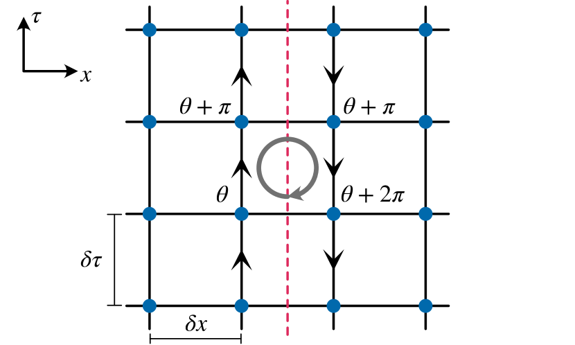
Figure 7: A vortex with $\nu=1$ resting a bond connecting two points $x_{j}$ and $x_{j+1}$ is shown. The spacetime is discretized to the rectangular lattice. The vorticity is defined on a rectangular plaquette indicated by a gray circle with an arrow. The $\theta$ field changes by $\pi$ along the vertical line with arrows. The vorticity on the plaquette is $\nu=[\theta(x,\tau+\delta\tau)-\theta(x,\tau)-\theta(x+\delta x,\tau+\delta\tau)+\theta(x+\delta x,\tau+\delta\tau)]/2\pi=1$.

The meron’s topological charge (105) is characterized by the two integers, $(\sigma,\nu)$, where $\sigma=\pm 1$ is the sign of $n^{z}$ at the center of the meron’s core and $\nu\in\mathbb{Z}$ is the vorticity density. In what follows, we discretize the ($1+1$)-dimensional spacetime as the rectangular lattice with the lattice spacings $\delta\tau$ and $\delta x$ in the $\tau$ and $x$ directions, respectively (Fig. 7). If we take $\delta\tau$ and $\delta x$ much larger than the core size of the meron, the meron on the discretized spacetime behaves just like the vortex except for the topological term. The topological charge (105) recalls the orientation $\sigma=\pm 1$ of $n^{z}$ at the core center of the meron. When the system has $N_{\mathrm{m}}$ merons with $(\sigma_{n},\nu_{n})$ for $n=1,2,\cdots,N_{\mathrm{m}}$, the net topological charge (105) is written as Nagaosa and Tokura (2013)

$$Q_{\rm m}=\sum_{n=1}^{N_{\mathrm{m}}}\frac{1}{2}\sigma_{n}\nu_{n}.$$ (106)

The vorticity density is defined as

$$\nu_{n} =\frac{\delta\tau\delta x}{2\pi}(\partial_{\tau}\partial_{x}-\partial_{x}\partial_{\tau})\theta(x,\tau).$$ (107)

The net vorticity over the system, $Q_{\rm v}$, is given by

$$Q_{\rm v} =\sum_{n}\nu_{n}=\frac{1}{2\pi}\int d\tau dx\,(\partial_{\tau}\partial_{x}-\partial_{x}\partial_{\tau})\theta(x,\tau).$$ (108)

We are now ready to derive a dual field theory of the O(3) NL$\sigma$M. The meron has a characteristic length scale $\ell_{\rm c}$ corresponding to the core size. If the correlation length, $\ell$, of merons is much longer than $\ell_{\rm c}$, the merons can be effectively regarded as vortices at the length scale $\gtrsim\ell$. We can assume $\ell\gg\ell_{\rm c}$ without loss of generality thanks to $D$. Larger $D/v$ shrinks the core size $\ell_{\rm c}$ and expands the correlation length $\ell$ simultaneously. Accordingly, we can construct the low-energy effective field theory of meron similarly to that for the vortex Kosterlitz and Thouless (1973); Kosterlitz (1974). Following the standard argument of the dual transformation of the two-dimensional XY model to the sine-Gordon theory Kosterlitz and Thouless (1973); Kosterlitz (1974), we rewrite the action $\mathcal{S}$ and the partition function $Z$ as

$$\mathcal{S} =\frac{1}{2g}\int d\tau dx\,(\partial_{\mu}\theta)^{2}-(\ln\zeta)\sum_{n=0}^{N_{\rm m}}\nu_{n}^{2}+i\frac{\Theta}{2}\sum_{n=0}^{N_{\rm m}}\sigma_{n}\nu_{n},$$ (109)

$$Z =\sum_{N_{\rm m}=0}^{\infty}\int\mathcal{D}\mathcal{\theta}\,\exp(-\mathcal{S}),$$ (110)

where $(\partial_{\mu}\theta)^{2}=(\partial_{x}\theta)^{2}+(\partial_{\tau}\theta)^{2}$ and $\zeta$ is a fugacity of the meron Affleck (1986). $N_{\rm m}=0,1,2,\cdots$ is the total number of merons. We set $\nu_{0}=\sigma_{0}=0$ for $N_{\mathrm{m}}=0$. Note that the velocity $v$ is set to unity for simplicity. We can resurrect $v$ whenever we want. The second term of Eq. (109) represents the energy cost to create the meron with $(\sigma_{n},\nu_{n})$, which is introduced here based on physical considerations Kosterlitz (1974). The energy cost is independent of $\sigma_{n}=\pm 1$ thanks to the global $\mathbb{Z}_{2}$ symmetry under $n^{z}\to-n^{z}$. The easy-plane anisotropy $D(n^{z})^{2}$ is encoded in the fugacity $\zeta$.

Let us introduce an auxiliary field $J_{\mu}$ for $\mu=\tau,x$ through the Hubbard-Stratonivich transformation Takayoshi et al. (2015).

$$Z =\sum_{N_{\rm m}}\int\mathcal{D}\theta\mathcal{D}J_{\tau}\mathcal{D}J_{x}\exp\biggl{(}-\frac{1}{2\pi K}\int d\tau dx\,{J_{\mu}}^{2}$$

$$\quad+\frac{i}{\pi}\int d\tau dx\,J_{\mu}\partial_{\mu}\theta+(\ln\zeta)\sum_{n}\nu_{n}^{2}-i\frac{\Theta}{2}\sum_{n}\sigma_{n}\nu_{n}\biggr{)},$$ (111)

with $K$ being

$$K =\frac{\pi}{g}.$$ (112)

Here, we split $\theta$ into a regular part $\theta_{\rm r}$ and a vortex part $\theta_{\rm v}$: $\theta=\theta_{\rm r}+\theta_{\rm v}$. These two parts are distinguished by the vorticity,

$$(\partial_{\tau}\partial_{x}-\partial_{x}\partial_{\tau})\theta_{\rm r}(x,\tau) =0,$$

$$(\partial_{\tau}\partial_{x}-\partial_{x}\partial_{\tau})\theta_{\rm v}(x,\tau) \not=0.$$ (113)

Integrating $\theta_{\rm r}$ field in Eq. (111), we obtain the delta function

$$\int\prod_{\tau,x}\mathcal{D}\theta_{\rm r}(x,\tau)\exp\biggl{(}-\frac{i}{\pi}(\partial_{\mu}J_{\mu})\theta_{\rm r}\biggr{)}\propto\prod_{\tau,x}\delta(\partial_{\mu}J_{\mu}).$$ (114)

On the other hand, completing the square with respect to $J_{\mu}$, we find that the following relation holds along a path with the largest contribution to the path integral:

$$J_{\mu}=iK\partial_{\mu}\theta_{\rm v},$$ (115)

for $\mu=\tau,x$. Hereafter, we denote $\theta_{\rm v}$ as $\theta$ for simplicity except when we stress the difference of $\theta_{\rm v}$ and $\theta$.

The condition, $\partial_{\mu}J_{\mu}=0$, imposed by the delta function $\delta(\partial_{\mu}J_{\mu})$ is automatically met if we write the $J_{\mu}$ field as

$$J_{\mu}=\varepsilon^{\mu\nu}\partial_{\nu}\phi,$$ (116)

where $\varepsilon^{\mu\nu}$ is the two-dimensional complete anatisymmetric tensor with $\varepsilon^{\tau x}=1$. The field $\phi$ introduced so is dual to $K\theta$ in a sense that they satisfy the Cauchy-Riemann relation,

$$\frac{K}{v}\partial_{t}\theta =\partial_{x}\phi,$$ (117)

$$-K\partial_{x}\theta =\frac{1}{v}\partial_{t}\phi.$$ (118)

The $\phi$ field is coupled to the vorticity density through the following term of the action (111):

$$\frac{i}{\pi}\int d\tau dx\,J_{\mu}\partial_{\mu}\theta =-\frac{i}{\pi}\int d\tau dx\,\varepsilon^{\mu\nu}\phi\partial_{\nu}\partial_{\mu}\theta.$$ (119)

We derived the right hand side by integrating $\phi$ by parts. If we discretize the spacetime to a rectangular lattice (Fig. 7), we can further rewrite it as

$$\exp\biggl{(}\frac{i}{\pi}\int d\tau dx\,J_{\mu}\partial_{\mu}\theta\biggr{)} =\prod_{\tau,x}\exp(2i\phi\nu_{n}).$$ (120)

We obtain the following expression of the partition function:

$$Z =\sum_{N_{\rm m}}\int\mathcal{D}\phi\prod_{\tau,x}\exp\biggl{(}-\frac{1}{2\pi K}(\partial_{\mu}\phi)^{2}+2i\phi\nu_{n}$$

$$\quad+(\ln\zeta)\nu_{n}^{2}-i\frac{\Theta}{2}\sigma_{n}\nu_{n}\biggr{)}.$$ (121)

Let us keep the $N_{\rm m}=0,1$ contributions only.

Since the larger $\nu_{n}$ requires larger energy cost to create the meron, we limit ourselves to $\nu_{n}=0$ or $\nu_{n}=\pm 1$ for $N_{\rm m}=1$. Then the partition function is approximated as

$$Z \approx\int\mathcal{D}\phi\prod_{\tau,x}\exp\biggl{(}-\frac{1}{2\pi K}(\partial_{\mu}\phi)^{2}\biggr{)}$$

$$\quad\times\biggl{[}1+\zeta(e^{2i\phi}+e^{-2i\phi})(e^{-i\frac{\Theta}{2}}+e^{i\frac{\Theta}{2}})\biggr{]}$$

$$\approx\int\mathcal{D}\phi\prod_{\tau,x}\exp\biggl{(}-\frac{1}{2\pi K}(\partial_{\mu}\phi)^{2}+4\zeta\cos(\Theta/2)\cos(2\phi)\biggr{)}$$

$$=\int\mathcal{D}\phi\exp(-\mathcal{S}_{\rm dual}),$$ (122)

with the dual action,

$$\mathcal{S}_{\rm dual} =\frac{v}{2\pi K}\int d\tau dx\,(\partial_{\mu}\phi)^{2}$$

$$\qquad-4\zeta\cos\biggl{(}\frac{\Theta}{2}\biggr{)}\int d\tau dx\,\cos(2\phi).$$ (123)

Since $\Theta=2\pi S$, the dual action (123) is consistent with the existence of the symmetric gapped quantum phase for $S\in\mathbb{Z}$. Besides, the sine-Gordon theory (123) shows that the Haldane phases for odd $S$ and even $S$ belong to different phases. The odd-spin Haldane phase is the symmetry-protected topological phase whereas the even-spin one is topologically trivial Pollmann et al. (2012).

When $S\in\mathbb{Z}+1/2$, the coupling constant vanishes, $\cos(\Theta/2)=\cos(\pi S)=0$. The merons with odd vorticities are then forbidden. Instead, the merons with even vorticities should be taken into account. The largest contribution comes from a pair of merons with $\nu_{1}=\nu_{2}=\pm 1$ Including these merons, we are led to

$$\mathcal{S}_{\rm dual} =\frac{v}{2\pi K}\int d\tau dx\,(\partial_{\mu}\phi)^{2}-4\zeta^{2}\cos\Theta\int d\tau dx\,\cos(4\phi),$$ (124)

for $S\in\mathbb{Z}+1/2$. When the ground state described by the sine-Gordon model (124) is gapped, the ground state is doubly degenerate due to the spontaneous breaking of the $\phi\to\phi+\pi/2$ symmetry. As we see below, this symmetry is the one-site translation symmetry of the spin chain.

B.3.2 Operator relations between spin and dual boson

To represent spin chain’s symmetries in terms of the dual boson field, $\phi$, we need a translation dictionary from the spin to the boson. Let us recall that the sine-Gordon theories (123) and (124) are derived from the NL$\sigma$M. Since we already have the translation rules (87) and (88) from the spin to the sigma field $\bm{n}$, we only need to establish the translation from the sigma field to the $\phi$ boson. If we completely ignore the quantum fluctuations, we find $\bm{\Omega}(x_{j})=(-1)^{j}\bm{n}(x_{j})$. With the polar coordinate,

$$\bm{n}(x,\tau) =\begin{pmatrix}\sin\gamma(x,\tau)\cos\theta(x,\tau)\\ \sin\gamma(x,\tau)\sin\theta(x,\tau)\\ \cos\gamma(x,\tau)\end{pmatrix}.$$ (125)

Note that we are focused on the physics at the length scale much longer than the core size. Almost everywhere is thus outside the meron’s core. The polar angle is fixed to $\gamma=\pi/2$ outside the core. At the classical level, we have $n^{x}=\cos\theta$ and $n^{y}=\sin\theta$ but the others, $n^{z}$, $L^{x}$, $L^{y}$, and $L^{z}$, are zero. The latter quantities become nonzero when the quantum fluctuation is taken into account.

Previously, we found an equation (95) to relate $\bm{L}$ to $\bm{n}$. For the $z$ component,

$$a_{0}L^{z} =\frac{a_{0}}{gv}(\bm{n}\times\partial_{t}\bm{n})^{z}$$

$$=\frac{a_{0}K}{\pi v}\partial_{t}\theta.$$ (126)

Using the Cauchy-Riemann relation (118), we obtain

$$a_{0}L^{z} =\frac{a_{0}}{\pi}\partial_{x}\phi.$$ (127)

The equal-time commutation relation, $[L^{z}(x),n^{a}(y)]=i\varepsilon^{zab}n^{b}(x)\delta(x-y)$ is then rephrased as $[\partial_{x}\phi(x),e^{i\theta(y)}]=\pi e^{i\theta(x)}\delta(x-y)$, which implies

$$[\partial_{x}\phi(x),\theta(y)] =\pi i\delta(x-y),$$ (128)

or equivalently,

$$[\phi(x),\partial_{y}\theta(y)] =\pi i\delta(x-y).$$ (129)

These commutation relations are exactly identical to the canonical one for the U(1) compact boson field of the TL liquid Giamarchi (2004) and also equivalent to Eq. (73).

Next, we look into $n^{z}$. This quantity is coupled to the staggered magnetic field through the Zeeman energy, $-h_{s}\sum_{j}(-1)^{j}S_{j}^{z}=-(Sh_{s}/a_{0})\int dx\,n^{z}(x)$. The staggered field makes merons with $\sigma=\pm$ nonequivalent. In other words, $h_{s}$ makes the fugacity dependent on $\sigma_{n}$: $\zeta_{\sigma_{n}}$. We can include the staggered field into the action (109) as follows.

$$\mathcal{S} =\frac{1}{2g}\int d\tau dx\,(\partial_{\mu}\theta)^{2}-\sum_{n=0}^{N_{\rm m}}(\ln\zeta_{\sigma_{n}})\nu_{n}^{2}$$

$$\qquad+i\frac{\Theta}{2}\sum_{n=0}^{N_{\rm m}}\sigma_{n}\nu_{n}.$$ (130)

Repeating the dual transformation, we obtain

$$Z \approx\int\mathcal{D}\phi\prod_{\tau,x}\exp\biggl{(}-\frac{1}{2\pi K}(\partial_{\mu}\phi)^{2}\biggr{)}$$

$$\quad\times\biggl{[}1+\zeta_{+}e^{2\phi i}e^{-i\frac{\Theta}{2}}+\zeta_{-}e^{2\phi i}e^{i\frac{\Theta}{2}}$$

$$\quad+\zeta_{+}e^{-2\phi i}e^{i\frac{\Theta}{2}}+\zeta_{-}e^{2\phi i}e^{-i\frac{\Theta}{2}}\biggr{]}$$

$$=\int\mathcal{D}\phi\prod_{\tau,x}\exp\biggl{(}-\frac{1}{2\pi K}(\partial_{\mu}\phi)^{2}\biggr{)}$$

$$\quad\times\biggl{[}1+2\zeta_{+}\cos\biggl{(}2\phi-\frac{\Theta}{2}\biggr{)}+2\zeta_{-}\cos\biggl{(}2\phi+\frac{\Theta}{2}\biggr{)}\biggr{]}$$

$$\approx\int\mathcal{D}\phi\prod_{\tau,x}\exp\biggl{(}-\frac{1}{2\pi K}(\partial_{\mu}\phi)^{2}\biggr{)}$$

$$\quad\times\biggl{[}1+2(\zeta_{+}+\zeta_{-})\cos\biggl{(}\frac{\Theta}{2}\biggr{)}\cos(2\phi)$$

$$\quad+2(\zeta_{+}-\zeta_{-})\sin\biggl{(}\frac{\Theta}{2}\biggr{)}\sin(2\phi)\biggr{]}.$$ (131)

Here, we expand the right hand side about $h_{s}$. The expansion of the fugacities $\zeta_{\pm}=\zeta\pm c_{\zeta}h_{s}$ with a constant $c_{\zeta}$ leads to

$$Z \approx\int\mathcal{D}\phi\prod_{\tau,x}\exp\biggl{(}-\frac{1}{2\pi K}(\partial_{\mu}\phi)^{2}\biggr{)}$$

$$\quad\times\biggl{[}1+4\zeta\cos\biggl{(}\frac{\Theta}{2}\biggr{)}\cos(2\phi)$$

$$\qquad+4c_{\zeta}h_{s}\sin\biggl{(}\frac{\Theta}{2}\biggr{)}\sin(2\phi)\biggr{]}$$

$$\approx\int\mathcal{D}\phi\,\exp(-\mathcal{S}_{\rm dual}).$$ (132)

The dual action is thus given by

$$\mathcal{S}_{\rm dual} =\frac{1}{2\pi K}(\partial_{\mu}\phi)^{2}-4\zeta\cos(\Theta/2)\cos(2\phi)$$

$$\quad+a_{1}h_{s}\sin(\Theta/2)\sin(2\phi),$$ (133)

with a constant $a_{1}$. The last term implies

$$n^{z} =a_{1}\sin(\Theta/2)\sin(2\phi).$$ (134)

Finally, we rewrite $L^{x}$ and $L^{y}$.

$$L^{x} =\frac{1}{gv}(n^{y}\partial_{t}n^{z}-n^{z}\partial_{t}n^{x})$$

$$=\frac{a_{1}}{gv}\sin(\Theta/2)\bigl{\{}\sin\theta(\partial_{t}\phi)\cos(2\phi)$$

$$\qquad-\sin(2\phi)(\partial_{t}\theta)\cos\theta\bigr{\}},$$ (135)

$$L^{y} =\frac{1}{gv}(n^{z}\partial_{t}n^{x}-n^{x}\partial_{t}n^{z})$$

$$=-\frac{a_{1}}{gv}\sin(\Theta/2)\bigl{\{}-\sin(2\phi)(\partial_{t}\theta)\sin\theta$$

$$\qquad-2\cos\theta(\partial_{t}\phi)\cos(2\phi)\bigr{\}}.$$ (136)

The operator-product expansion of the $\phi$ field Di Francesco et al. (1998),

$$\partial_{t}\phi(x+a_{0})\cos(2\phi(x)) =\frac{1}{ia_{0}}\sin(2\phi(x))+\cdots,$$ (137)

and a similar expansion for $\theta$ lead to

$$L^{x} =-ib_{1}\sin(\Theta/2)\sin\theta\sin(2\phi),$$ (138)

$$L^{y} =ib_{1}\sin(\Theta/2)\cos\theta\sin(2\phi),$$ (139)

with a constant $b_{1}\in\mathbb{R}$.

We could finally translate the spin operator into the $\phi$ and $\theta$ terms.

$$S_{j}^{z} =\frac{a_{0}}{\pi}\partial_{x}\phi+(-1)^{j}a_{1}\sin(\pi S)\sin(2\phi),$$ (140)

$$S_{j}^{+} =e^{i\theta}\bigl{[}(-1)^{j}+b_{1}\sin(\pi S)\sin(2\phi)\bigr{]}.$$ (141)

The dimer order parameter $(-1)^{j}\bm{S}_{j}\cdot\bm{S}_{j+1}$ is bosonized as

$$(-1)^{j}\bm{S}_{j}\cdot\bm{S}_{j+1}=d\cos(2\phi)+\cdots$$ (142)

with a nonuniversal constant $d\in\mathbb{R}$ Orignac (2004); Takayoshi and Sato (2010); Hikihara et al. (2017); Berg et al. (2008). This bosonization formula follows from operator product expansions such as

$$(-1)^{j}S_{j}^{z}S_{j+1}^{z} \approx\frac{2a_{0}a_{1}}{\pi}\partial_{x}\phi\sin(2\phi(x+a_{0}))+\cdots$$

$$\sim\cos(2\phi(x))+\cdots.$$ (143)

Surprisingly, Eqs. (140), (141), and (142) are identical to the standard bosonizaton formulas Giamarchi (2004) for $S=1/2$. We call Eqs. (140) and (141) semiclassical bosonization formulas. The relations (140) and (141) imply that $\phi$ and $\theta$ for $S\in\mathbb{Z}+1/2$ are compactified as

$$\phi\sim\phi+\pi,\qquad\theta\sim\theta+2\pi.$$ (144)

Note that the staggered component of Eq. (140) vanishes when $S\in\mathbb{Z}$. The staggered component is not absent but represented as $\sin\phi$ for $S\in\mathbb{Z}$. This $S$ dependence of the bosonization formulas is related to the LSM theorem Lieb et al. (1961); Furuya and Oshikawa (2017). For $S\in\mathbb{Z}+1/2$, the anisotropy $D(n^{z})^{2}\propto-\cos(4\phi)$ does not induce the unique gapped ground state. If $\cos(4\phi)$ is relevant and makes the ground state gapped, the ground state breaks the one-site translation symmetry, $\phi\to\phi+\frac{\pi}{2}$, spontaneously, as we see soon later. For $S\in\mathbb{Z}$, by contrast, $D(n^{z})^{2}$ with large enough $D>0$ makes the unique gapped ground state, which is the large-$D$ state, $\bigotimes_{j}\ket{S_{j}^{z}=0}$. The effective Hamiltonian (123) implies that $D(n^{z})^{2}\propto-D\cos(2\phi)$. Here, the minus sign comes from the fact that the large-$D$ phase is topologically trivial. We can deduce

$$n^{z}\propto\sin\phi,\qquad(S\in\mathbb{Z}),$$ (145)

for $S\in\mathbb{Z}$. Equation (145) is consistent with the $S$ dependence of the one-site translation symmetry. According to Eq. (140), the one-site translation $T_{1}:\,\bm{S}_{j}\to\bm{S}_{j+1}$ can be rephrased as

$$T_{1}:\quad\phi(x)\to\phi(x)+\frac{\pi}{2}\mod\pi,$$ (146)

for $S\in\mathbb{Z}+1/2$. On the other hand, $T_{1}$ should act on $\phi$ for $S\in\mathbb{Z}$ as

$$T_{1}:\quad\phi(x)\to\phi(x)+\pi\mod\pi,$$ (147)

for $S\in\mathbb{Z}$ because the effective field theory (61) is $T_{1}$-invariant and also because the integer-spin HAFM chain can be seen as a two-leg HAFM ladder of the half-odd-integer spin Fuji (2016). For $S\in\mathbb{Z}$, the two boson fields $\phi$ and $\theta$ will be compactified as

$$\phi\sim\phi+\pi,\qquad\theta\sim\theta+2\pi.$$ (148)

This compactification of $\phi$ is consistent with the deduced relation (145). However, unfortunately, no microscopic derivations of Eq. (145) are yet available.

In the main text, we discuss the symmetry protection of the quantization of the edge magnetization. In the spin-$S$ chains, the protecting symmetries are the U(1) spin-rotation symmetry and the site-centered inversion symmetry. The rotation around the $z$ axis by an angle $\varphi$ is obviously translated into

$$\phi(x) \to\phi(x),\qquad\theta(x)\to\theta(x)+\varphi.$$ (149)

The site-centered inversion symmetry is

$$\phi(x) \to-\phi(L-x)+\pi S,\qquad\theta(x)\to\theta(L-x).$$ (150)

The symmetries (149) and (150) forbid $\cos\theta$, $\sin\theta$, and $\cos(2\phi)$ for the $S\in\mathbb{Z}+1/2$ case (3) and forbids $\cos\theta$, $\sin\theta$, and $\sin(2\phi)$ for the $S\in\mathbb{Z}$ case (33).

Appendix C Semiclassical bosonization on magnetization plateaus

C.1 Classical Hamiltonian of nonlinear sigma model

Our starting point for $m>0$ is also the relation (88). For $m=0$, we first considered the classical Néel configuration and took the quantum fluctuation into account later. On the magnetization plateau with $m>0$, instead, the classical configuration is the transverse Néel state with the longitudinal uniform magnetization:

$$\bm{\Omega}(x_{j},\tau) =\begin{pmatrix}(-1)^{j}n^{x}(x_{j},\tau)\sqrt{1-(m/S)^{2}}\\ (-1)^{j}n^{y}(x_{j},\tau)\sqrt{1-(m/S)^{2}}\\ m/S\end{pmatrix}$$

$$=\begin{pmatrix}(-1)^{j}\sin\gamma_{0}\cos\theta(x_{j},\tau)\\ (-1)^{j}\sin\gamma_{0}\sin\theta(x_{j},\tau)\\ \cos\gamma_{0}\end{pmatrix},$$ (151)

where $\cos\gamma_{0}=m/S$ is fixed to a constant.

In Sec. B, the staggered part $(-1)^{j}\bm{n}(x_{j})$ of $\bm{\Omega}(x_{j})$ is the classical configuration and the uniform part $(a_{0}/S)\bm{L}(x_{j})$ is the quantum fluctuation. In this section, we regard Eq. (151) as the classical configuration and the other part of $\bm{\Omega}(x_{j},\tau)$,

$$\begin{pmatrix}(a_{0}/S)L^{x}\\ (a_{0}/S)L^{y}\\ (-1)^{j}n^{z}(x_{j},\tau)\sqrt{1-(m/S)^{2}}\end{pmatrix},$$ (152)

as the quantum fluctuation.

Similarly to Sec. B, we also consider the spin-$S$ HAFM chain,

$$\mathcal{H}=J\sum_{j}\bm{S}_{j}\cdot\bm{S}_{j+1}-h_{u}\sum_{j}S_{j}^{z}.$$ (153)

The classical Hamiltonian, $\mathcal{H}_{\rm cl}$, in the path integral formalism is almost identical to Eq. (94):

$$\mathcal{H}_{\rm cl} =\int\frac{dx}{a_{0}}\biggl{(}\frac{JS^{2}{a_{0}}^{2}}{2}(\partial_{x}\bm{n})^{2}+2J{a_{0}}^{2}\bm{L}^{2}$$

$$\quad-h_{u}(a_{0}L^{z}+{a_{0}}^{2}\partial_{x}L^{z})\biggr{)}+\mathrm{const.}$$

$$=\int dx\biggl{(}\frac{v}{2g}(\partial_{x}\bm{n})^{2}+\frac{gv}{2}\bm{L}^{2}-h_{u}L^{z}\biggr{)}+\mathrm{const.}$$ (154)

The Heisenberg equation of motion for $\bm{n}$ relates $\bm{L}$ and $\partial_{t}\bm{n}$:

$$\bm{L} =\frac{1}{gv}\bm{n}\times(\partial_{t}\bm{n}+\bm{h}_{u}\times\bm{n}),$$ (155)

with $\bm{h}_{u}=(0\>0\>h_{u})^{T}$. The uniform magnetic field $h_{u}$ is fixed so that $a_{0}h_{u}/gv=m$.

C.2 Berry phase

At first glance, the classical Hamiltonian $\mathcal{H}_{\rm cl}$ does not make much difference from that for $m=0$. By contrast, the Berry phase is completely different. The value of the Berry phase is insensitive to the local modifications of $\bm{\Omega}(x_{j},\tau)$ thanks to its topological nature. Accordingly, the Berry phase is governed by the classical configuration in the semiclassical approach.

In what follows, we rewrite the Berry phase of the classical configuration (151). Note that the following argument just repeats those of Refs. Lamas et al. (2011); Takayoshi et al. (2015). Still, it is worth repeating here because we are to derive the Berry phase later in similar but more extended situations.

First, we note that the Berry phase for the classical configuration (151) of $\bm{\Omega}(x_{j})$ is identical to that for another configuration $\tilde{\bm{\Omega}}(x_{j},\tau)$, that is,

$$\tilde{\bm{\Omega}}(x_{j},\tau) =\begin{pmatrix}\sin\gamma_{0}\cos\theta(x_{j},\tau)\\ \sin\gamma_{0}\sin\theta(x_{j},\tau)\\ \cos\gamma_{0}\end{pmatrix},$$ (156)

except for a certain constant. More precisely Tanaka et al. (2009),

$$-iS\sum_{j}\omega[\bm{\Omega}(x_{j},\tau)] =-iS\sum_{j}\omega[\tilde{\bm{\Omega}}(x_{j},\tau)]+i\pi\sum_{j}(S-m).$$ (157)

Since the second term on the right-hand side is merely a constant, we can identify these two Berry phases.

Next, following Ref. Takayoshi et al. (2015), we rewrite the Berry phase for $\tilde{\bm{\Omega}}$ as follows.

$$\mathcal{S}_{\rm BP} =-iS\sum_{j=1}^{L}\omega[\tilde{\bm{\Omega}}(x_{j},\tau)]$$

$$=-iS\sum_{j^{\prime}=1}^{L/2}\omega[\tilde{\bm{\Omega}}(x_{2j^{\prime}},\tau)]-iS\sum_{j^{\prime}=1}^{L/2}\biggl{(}2(1-\cos\gamma_{0})\int_{0}^{\beta}d\tau\,\partial_{\tau}\theta(x_{2j^{\prime}-1},\tau)-\omega[\tilde{\bm{\Omega}}(x_{2j^{\prime}-1},\tau)]\biggr{)}$$

$$=-iS\sum_{j=1}^{L}(-1)^{j}\omega[\tilde{\bm{\Omega}}(x_{j},\tau)]-2i(S-m)\sum_{j^{\prime}=1}^{L/2}\int_{0}^{\beta}d\tau\,\partial_{\tau}\theta(x_{2j^{\prime}-1},\tau)$$

$$=i\pi(S-m)Q_{\rm v}-i(S-m)\int_{0}^{L}\frac{dx}{a_{0}}\int_{0}^{\beta}d\tau\,\partial_{\tau}\theta(x,\tau)$$ (158)

In the last line, we used the one-site translation symmetry. $Q_{\rm v}=\sum_{n}\nu_{n}$ represents the net vorticity on the two-dimensional spacetime, (108). We arrived at the following form of the Berry phase.

$$\mathcal{S}_{\rm BP} =i\pi(S-m)Q_{\rm v}+\mathcal{S}_{\rm LSM},$$ (159)

$$\mathcal{S}_{\rm LSM} =-i(S-m)\int_{0}^{L}\frac{dx}{a_{0}}\int_{0}^{\beta}d\tau\,\partial_{\tau}\theta(x,\tau).$$ (160)

As Ref. Takayoshi et al. (2015) mentioned, the term (160) is related to the LSM theorem Lieb et al. (1961). Let us denote the ground state on the magnetization plateau as $\ket{\psi_{0}}$. The ground state has a configuration, $\{\theta(x,\tau)\}_{\{x,\tau\}\in\mathbb{R}^{2}}$, of the $\theta$ field. Here, we consider another state, $\ket{\psi_{1}}$, with a slowly shifted configuration $\{\theta^{\prime}(x,\tau)\}_{\{x,\tau\}\in\mathbb{R}^{2}}$, related to $\theta(x,\tau)$ through

$$\theta^{\prime}(x,\tau) =\theta(x,\tau)-\frac{2\pi a_{0}}{\beta L}\tau.$$ (161)

The $\theta^{\prime}$ field respects the periodic boundary condition only in the $L\to+\infty$ limit since $\theta^{\prime}(x,\tau+\beta)=\theta^{\prime}(x,\tau)-2\pi a_{0}/L$. Nevertheless, it is useful to consider the shifted field $\theta^{\prime}$ because it works as a variational configuration of the genuine low-energy state.

The analytical continuation $\tau\to it$ clarifies the physical meaning of the shift (161). The shift $i(2\pi a_{0}/\beta L)t$ of $\theta$ is an insertion of a gauge field $\bm{A}=(A_{0},A_{1})$ with

$$A_{0} =0,$$ (162)

$$A_{1} =\frac{2\pi a_{0}}{\beta L}t,$$ (163)

in the real time $t$ Yao and Oshikawa (2020). The gauge field is gradually increased from the time $t=0$ to $t=\beta$, that is, $A_{1}(t=0)=0$ and $A_{1}(t=\beta)=2\pi a_{0}/L$. The latter corresponds to the unit flux insertion Furuya and Nakamura (2019). The gauge field is adiabatically inserted in the $\beta\to+\infty$ limit.

The state $\ket{\psi_{1}}$ has a vanishing excitation energy in the thermodynamic limit at zero temperature because the difference of the classical energies,

$$\mathcal{H}_{\rm cl}[\theta^{\prime}]-\mathcal{H}_{\rm cl}[\theta] =-\frac{2vK}{\beta L}\int_{0}^{L}dx\,\partial_{x}\theta(x,\tau)$$

$$\qquad+\frac{L}{a_{0}}\frac{vK}{2\pi}\biggl{(}\frac{2\pi a_{0}}{\beta L}\biggr{)}^{2},$$ (164)

is vanishing in the limit of $L\to+\infty$.

However, the shift (161) affects the LSM term.

$$\mathcal{S}_{\rm LSM} =-i(S-m)\int_{0}^{L}\frac{dx}{a_{0}}\int_{0}^{\beta}d\tau\,\partial_{\tau}\theta^{\prime}(x,\tau)$$

$$=-i(S-m)\int_{0}^{L}\frac{dx}{a_{0}}\int_{0}^{\beta}d\tau\,\partial_{\tau}\theta(x_{j},\tau)+2\pi i(S-m).$$ (165)

If $S-m\not\in\mathbb{Z}$, the two states, $\ket{\psi_{0}}$ and $\ket{\psi_{1}}$, belong to different topological sectors. When $S-m=p/q$ for coprime integers $p$ and $q$, there are $q$ orthogonal low-energy states, $\ket{\psi_{0}},\,\ket{\psi_{1}},\,\cdots,\ket{\psi_{q-1}}$. The low-energy state $\ket{\psi_{n}}$ for $n>0$ has the configuration,

$$\theta^{\prime}(x,\tau) =\theta(x,\tau)-\frac{2\pi a_{0}}{\beta L}n\tau.$$ (166)

Therefore, when $S-m\in\mathbb{Z}+p/q$, the partition function at zero temperature is given by

$$Z \approx\sum_{n=0}^{q-1}\braket{\psi_{n}}{e^{-\beta\mathcal{H}}}{\psi_{n}}.$$ (167)

C.3 Dual transformation to sine-Gordon theory

C.3.1 When $S-m\in\mathbb{Z}$

Here, we consider the simplest case of $S-m\in\mathbb{Z}$. The $m\not=0$ case starts from the classical configuration (151). Unlike the $m=0$ case, the topological excitation is the vortex rather than the meron. Note that the path integral is defined under the (imaginary-)temporal boundary condition:

$$\theta(\tau+\beta,x)=\theta(\tau,x)\mod 2\pi.$$ (168)

The LSM term (160) does not interfere with the boundary condition (168) for $S-m\in\mathbb{Z}$ and is thus negligible. For $S-m\in\mathbb{Z}$, the dual field theory is derived as follows. The classical configuration,

$$n^{x} =\sqrt{1-(m/S)^{2}}\,\cos\theta(x,\tau),$$ (169)

$$n^{y} =\sqrt{1-(m/S)^{2}}\,\sin\theta(x,\tau),$$ (170)

$$a_{0}L^{z} =m,$$ (171)

leads to the following action,

$$\mathcal{S} =\frac{v[1-(m/S)^{2}]}{2g}\int d\tau dx\,(\partial_{\mu}\theta)^{2}-(\ln\zeta)\sum_{n=0}^{N_{\rm v}}\nu_{n}^{2}$$

$$\qquad-i\pi(S-m)\sum_{n=0}^{N_{\rm v}}\nu_{n}$$

$$=\frac{vK}{2\pi}\int d\tau dx\,(\partial_{\mu}\theta)^{2}-(\ln\zeta)\sum_{n=0}^{N_{\rm v}}\nu_{n}^{2}$$

$$\qquad-i\pi(S-m)\sum_{n=0}^{N_{\rm v}}\nu_{n},$$ (172)

with the Luttinger parameter,

$$K =\frac{\pi}{g}[1-(m/S)^{2}].$$ (173)

$N_{\rm v}=0,1,2,\cdots$ is the number of vortices. The Hubbard-Stratonovich transformation turns the partition function into

$$Z =\sum_{N_{\rm v}}\int\mathcal{D}\theta\mathcal{D}J_{\tau}\mathcal{D}J_{x}\,\exp\biggl{(}-\frac{1}{2\pi K}\int d\tau dx\,{J_{\mu}}^{2}$$

$$\quad+\frac{i}{\pi}\int d\tau dx\,J_{\mu}\partial_{\mu}\theta+(\ln\zeta)\sum_{n=0}^{N_{\rm v}}\nu_{n}^{2}+\mathcal{S}_{\rm BP}\biggr{)}$$

$$=\sum_{N_{\rm v}=0}^{\infty}\int\mathcal{D}\phi\,e^{-\mathcal{S}_{\rm LSM}}\prod_{\tau,x}\exp\biggl{(}-\frac{1}{2\pi K}(\partial_{\mu}\phi)^{2}+2i\phi\nu_{n}$$

$$\quad+(\ln\zeta)\nu_{n}^{2}+\pi i(S-m)\nu_{n}\biggr{)}.$$ (174)

Collecting the $N_{\rm v}=0,1$ terms, we obtain the following representation of the partition function,

$$Z \approx\int\mathcal{D}\phi\prod_{\tau,x}\exp\biggl{(}-\frac{1}{2\pi K}(\partial_{\mu}\phi)^{2}\biggr{)}$$

$$\qquad\times\biggl{[}1+\zeta(e^{i[\pi(S-m)+2\phi]}+\mathrm{H.c.})\biggr{]}$$

$$=\int\mathcal{D}\phi\prod_{\tau,x}\exp(-\mathcal{S}_{\rm dual}),$$ (175)

with the dual action

$$\mathcal{S}_{\rm dual} =\frac{v}{2\pi K}\int d\tau dx\,(\partial_{\mu}\phi)^{2}$$

$$\qquad-2\zeta\int d\tau dx\,\cos[\pi(S-m)+2\phi]$$

$$=\frac{v}{2\pi K}\int d\tau dx\,(\partial_{\mu}\phi)^{2}$$

$$\qquad-2\zeta\cos[\pi(S-m)]\int d\tau dx\,\cos(2\phi).$$ (176)

Though the dual action is qualitatively the same as Eq. (140), they have two quantitative differences. The first difference is the coupling constant of the cosine interaction, where $\Theta=2\pi S$ is replaced by $2\pi(S-m)$. The other is the Luttinger parameter (173).

Let us compile the translation dictionary from the spin to the boson. We again start with $L^{z}$, which admits the following quantum fluctuation:

$$a_{0}L^{z} =m+\frac{a_{0}}{gv}(\bm{n}\times\partial_{t}\bm{n})^{z}$$

$$=m+\frac{a_{0}K}{\pi v}\partial_{t}\theta$$

$$=m+\frac{a_{0}}{\pi}\partial_{x}\phi.$$ (177)

Previously, we saw that the sine-Gordon theory at $m=0$ admits the staggered magnetic field $h_{s}$ as the imbalance of the fugacities of merons. This time, however, the staggered field hardly affects the fugacities of vortices, because the vortices have no longitudinal $n^{z}$ component classically. Instead, the staggered magnetic field is introduced to the action of the vortex through $m$. The staggered field modifies $m$ to $m+(-1)^{j}\delta m$. The staggered field doubles the unit-cell size of the spin-$S$ HAFM chain. The unit cell contains two sites, $x_{2j^{\prime}-1}$ and $x_{2j^{\prime}}$. The staggered magnetic field modifies the classical configuration to

$$\bm{\Omega}(x_{2j^{\prime}-1},\tau) =\begin{pmatrix}-\sqrt{1-[(m-\delta m)/S]^{2}}\cos\theta_{1}(x_{2j^{\prime}-1},\tau)\\ -\sqrt{1-[(m-\delta m)/S]^{2}}\sin\theta_{1}(x_{2j^{\prime}-1},\tau)\\ (m-\delta m)/S\end{pmatrix},$$ (178)

$$\bm{\Omega}(x_{2j^{\prime}},\tau) =\begin{pmatrix}\sqrt{1-[(m+\delta m)/S]^{2}}\cos\theta_{2}(x_{2j^{\prime}},\tau)\\ \sqrt{1-[(m+\delta m)/S]^{2}}\sin\theta_{2}(x_{2j^{\prime}},\tau)\\ (m+\delta m)/S\end{pmatrix}.$$ (179)

Doubling the unit-cell size also doubles the number of fields. Note that $\theta_{1}+\theta_{2}$ is related to the global U(1) spin-rotation symmetry but $\theta_{1}-\theta_{2}$ is unrelated to any global symmetry. Under such circumstance, the antisymmetric field, $\theta_{1}-\theta_{2}$, acquires the larger excitation gap than the symmetric field, $\theta_{1}+\theta_{2}$, does Oshikawa et al. (1997). Integrating out the high-energy antisymmetric field imposes a constraint,

$$\theta_{1}(x,\tau) =\theta_{2}(x,\tau)=\theta(x,\tau)\mod 2\pi.$$ (180)

This relation allows us to calculate the Berry phase in analogy with Eq. (158). Namely, the staggered magnetization leads to the Berry phase:

$$\mathcal{S}_{\rm BP} =-iS\sum_{j^{\prime}=1}^{L/2}\omega[\bm{\Omega}(x_{2j^{\prime}},\tau)]-iS\sum_{j^{\prime}=1}^{L/2}\biggl{[}2\biggl{(}1-\frac{m+\delta m}{S}\biggr{)}\int_{0}^{\beta}d\tau\,\partial_{\tau}\theta_{1}(x_{2j^{\prime}-1},\tau)-\omega[\bm{\Omega}(x_{2j^{\prime}-1},\tau)]\biggr{]}$$

$$=-iS\sum_{j=1}^{L}(-1)^{j}\omega[\bm{\Omega}(x_{j},\tau)]-2i(S-m-\delta m)\sum_{j^{\prime}=1}^{L/2}\int_{0}^{\beta}d\tau\,\partial_{\tau}\theta(x_{2j^{\prime}-1},\tau)$$

$$=\pi i(S-m-\delta m)Q_{\rm v}-i(S-m)\int_{0}^{L}\frac{dx}{a_{0}}\int_{0}^{\beta}d\tau\,\partial_{\tau}\theta(x,\tau).$$ (181)

The constant shift $S-m\to S-m-\delta m$ of the coefficient of $Q_{\rm v}$ affects the dual action as follows.

$$\mathcal{S}_{\rm dual} =\frac{v}{2\pi K}\int d\tau dx\,(\partial_{\mu}\phi)^{2}$$

$$\quad-2\zeta\int d\tau dx\,\cos[\pi(S-m-\delta m)-2\phi]$$

$$\approx\frac{v}{2\pi K}\int d\tau dx\,(\partial_{\mu}\phi)^{2}$$

$$\quad-2\zeta\int d\tau dx\,\cos[\pi(S-m)]\cos(2\phi)$$

$$\quad+2\zeta\delta m\int d\tau dx\,\cos[\pi(S-m)]\sin(2\phi).$$ (182)

The last term implies that $n^{z}$ is given by

$$n^{z} \propto(-1)^{j}\cos[\pi(S-m)]\sin(2\phi).$$ (183)

$L^{x}$, $L^{y}$ are obtained similarly to Eqs. (138) and (139). In short, we obtain

$$S_{j}^{z} =m+\frac{a_{0}}{\pi}\partial_{x}\phi+(-1)^{j}a_{1}\cos[\pi(S-m)]\sin(2\phi),$$ (184)

$$S_{j}^{+} =e^{i\theta}\bigl{[}(-1)^{j}+b_{1}\cos[\pi(S-m)]\sin(2\phi)\bigr{]},$$ (185)

with nonuniversal constants, $a_{1},b_{1}\in\mathbb{R}$. The semiclassical bosonization formulas (184) and (185) are identical to the $m=0$ ones (140) and (141) by replacing $\sin(\pi S)$ with $\cos[\pi(S-m)]$. The bosonization formulas (184) and (185) indicate that the one-site translation $T_{1}:\bm{S}_{j}\to\bm{S}_{j+1}$ and the site-centered inversion $\mathcal{I}_{s}:\bm{S}_{j}\to\bm{S}_{L-j}$ act on $\phi$ and $\theta$ as

$$T_{1} :\,\phi(x,\tau)\to\phi(x,\tau)+\frac{\pi}{2},$$ (186)

$$T_{1} :\,\theta(x,\tau)\to\theta(x,\tau)+\pi,$$ (187)

and

$$\mathcal{I}_{s} :\,\phi(x,\tau)\to-\phi(L-x,\tau)+\frac{\pi}{2},$$ (188)

$$\mathcal{I}_{s} :\,\theta(x,\tau)\to\theta(L-x,\tau)+\pi.$$ (189)

Since the bond-centered inversion $\mathcal{I}_{b}=T_{1}\mathcal{I}_{s}$ keeps the spin-rotation symmetries and inverts $\phi(x,\tau)\to-\phi(L-x,\tau)$, the dimer order parameter $(-1)^{j}\bm{S}_{j}\cdot\bm{S}_{j+1}$ is again bosonized as

$$(-1)^{j}\bm{S}_{j}\cdot\bm{S}_{j+1} =d\cos(2\phi)+\cdots.$$ (190)

C.3.2 When $S-m\in\mathbb{Z}+p/q$

When $S-m$ has a decimal part, we need to include the LSM-twisted states [Eq. (167)]. If we include the vortices with $\nu=\pm 1$ only, the partition function would become

$$Z \approx\int\mathcal{D}\phi\prod_{\tau,x}\exp\biggl{(}-\frac{1}{2\pi K}(\partial_{\mu}\phi)^{2}\biggr{)}$$

$$\quad\times\sum_{n=0}^{q-1}\biggl{[}1+e^{i\frac{2\pi n}{q}}\zeta(e^{i[\pi(S-m)-2\phi]}+e^{-i[\pi(S-m)-2\phi]})\biggr{]}$$

$$=\int\mathcal{D}\phi\prod_{\tau,x}\exp\biggl{(}-\frac{1}{2\pi K}(\partial_{\mu}\phi)^{2}\biggr{)},$$ (191)

because $\sum_{n=0}^{q}e^{i(2\pi n/q)}=0$. The LSM term thus forbids the single-vortex excitation with $\nu=\pm 1$. Likewise, it forbids those with $\nu\not=0\mod q$. Therefore, vortices can be excited only when $\nu_{n}\in q\mathbb{Z}$. The dual action is then given by

$$\mathcal{S}_{\rm dual} =\frac{v}{2\pi K}\int d\tau dx\,(\partial_{\mu}\phi)^{2}$$

$$\qquad-2\zeta\int d\tau dx\,\cos[\pi q(S-m)-2q\phi]$$

$$=\frac{v}{2\pi K}\int d\tau dx\,(\partial_{\mu}\phi)^{2}$$

$$\qquad-2\zeta\cos[\pi q(S-m)]\int d\tau dx\,\cos(2q\phi).$$ (192)

This field theory is perfectly consistent with the one discussed by Oshikawa, Yamanaka, and Affleck Oshikawa et al. (1997).

C.3.3 When $S-m\in\mathbb{Z}+1/2$

In the main text, the semiclassical bosonization formulas are required for the $S-m\in\mathbb{Z}+1/2$ case. In what follows, we limit ourselves to the $S-m\in\mathbb{Z}+1/2$ case.

To derive the semiclassical bosonization formulas, we need to investigate the response of the dual field theory to the external staggered magnetic field. There is a low-energy state, $\ket{\psi^{\prime}_{0}}$, that lives in a different topological sector from the ground state $\ket{\psi_{0}}$ for $\delta m=0$. Previously, we defined $\ket{\psi^{\prime}_{0}}=\ket{\psi_{1}}$ by twisting the $\theta$ field [Eq. (161)]. When $Q_{\rm v}=\pm 1$ and $S-m\in\mathbb{Z}+1/2$, we can instead employ another, more convenient, example of a low-energy state $\ket{\psi^{\prime}_{0}}$, that is,

$$\ket{\psi^{\prime}_{0}} =\mathcal{I}_{b}\ket{\psi_{0}}.$$ (193)

The bond-centered inversion flips the sign of the vorticity density,

$$\mathcal{I}_{b}:\,\nu_{n}\to-\nu_{n}.$$ (194)

Figure 7 gives a schematic understanding of the relation (194).

The $2i\phi\nu_{n}$ term of Eq. (174) is invariant under $\mathcal{I}_{b}$ because this term is originally $iJ_{\mu}\partial_{\mu}\theta_{\rm v}/\pi=-K(\partial_{\mu}\theta_{\rm v})^{2}/\pi$, which is apparently $\mathcal{I}_{b}$-invariant. To compensate this sign and make this term $\mathcal{I}_{b}$-invariant, the $\phi$ field must transform as

$$\mathcal{I}_{b}:\,\phi(x)\to-\phi(L-x)\mod 2\pi.$$ (195)

The relation (194) results in an interesting fact that $\ket{\psi_{0}}$ and $\ket{\psi^{\prime}_{0}}$ belong to different topological sectors because

$$\mathcal{I}_{b}\mathcal{S}_{\rm BP}\mathcal{I}_{b}^{-1} =-iS\sum_{j=1}^{L}(-1)^{j}\omega[\tilde{\bm{\Omega}}(x_{L+1-j},\tau)]$$

$$\quad-2i(S-m)\sum_{j^{\prime}=1}^{L/2}\int_{0}^{\beta}d\tau\,\partial_{\tau}\theta(x_{L+1-(2j^{\prime}-1)},\tau)$$

$$=iS\sum_{j=1}^{L}(-1)^{j}\omega[\tilde{\bm{\Omega}}(x_{j},\tau)]$$

$$\quad-2i(S-m)\sum_{j^{\prime}=1}^{L/2}\int_{0}^{\beta}d\tau\,\partial_{\tau}\theta(x_{2j^{\prime}},\tau)$$

$$=\mathcal{S}_{\rm BP}-2\pi i(S-m)Q_{\rm v}.$$ (196)

If $Q_{\rm v}=1$ and $S-m\in\mathbb{Z}+1/2$, the following relation holds:

$$\mathcal{I}_{b}\mathcal{S}_{\rm BP}\mathcal{I}_{b}^{-1}-\mathcal{S}_{\rm BP} =\pi i\mod 2\pi i.$$ (197)

The two states $\ket{\psi_{0}}$ and $\mathcal{I}_{b}\ket{\psi_{0}}$ are thus orthogonal low-energy states, equally contributing to the partition function,

$$Z =\braket{\psi_{0}}{e^{-\beta\mathcal{H}}}{\psi_{0}}+\braket{\psi^{\prime}_{0}}{e^{-\beta\mathcal{H}}}{\psi^{\prime}_{0}}$$

$$=\braket{\psi_{0}}{e^{-\beta\mathcal{H}}}{\psi_{0}}+\braket{\psi_{0}}{\mathcal{I}_{b}^{-1}e^{-\beta\mathcal{H}}\mathcal{I}_{b}}{\psi_{0}}.$$ (198)

When collecting the $N_{\rm v}=0,1$ terms, we find

$$Z \approx\int\mathcal{D}\phi\prod_{\tau,x}\exp\biggl{(}-\frac{v}{2\pi K}(\partial_{\mu}\phi)^{2}\biggr{)}$$

$$\quad\times\biggl{[}1+\zeta(e^{i[\pi(S-m)-2\phi]}+\mathrm{H.c.})$$

$$\quad-\zeta(e^{i[\pi(S-m)-2\phi]}+\mathrm{H.c.})\biggr{]}$$

$$=\int\mathcal{D}\phi\prod_{\tau,x}\exp\biggl{(}-\frac{v}{2\pi K}(\partial_{\mu}\phi)^{2}\biggr{)}.$$ (199)

The $N_{\rm v}=2$ term needs to be included to the action in order to generate the most relevant interaction. The dual action thus becomes

$$\mathcal{S}_{\rm dual} =\frac{v}{2\pi K}\int d\tau dx\,(\partial_{\mu}\phi)^{2}$$

$$\qquad-2\zeta^{2}\cos[2\pi(S-m)]\int d\tau dx\,\cos(4\phi).$$ (200)

If the ground state of the spin-1 HAFM chain for $S-m=1/2$ is gapped, it must be doubly degenerate by spontaneously breaking the $\phi\to\phi+\frac{\pi}{2}$ symmetry. The $\phi\to\phi+\frac{\pi}{2}$ symmetry is highly likely to be the one-site translation symmetry. If so, the site-centered inversion symmetry $\mathcal{I}_{s}=\mathcal{I}_{b}T_{1}$ acts on $\phi(x,\tau)$ as

$$\mathcal{I}_{s}:\,\phi(x)\to-\phi(L-x)+\frac{\pi}{2}\mod 2\pi.$$ (201)

Like $\mathcal{I}_{b}$, the site-centered inversion $\mathcal{I}_{s}=\mathcal{I}_{b}T_{1}$ flips the sign of $\nu_{n}\to-\nu_{n}$ because $T_{1}$ keeps $\nu_{n}$. An extra phase arises from the coupling $2i\phi\nu_{n}$ in Eq. (174). In fact,

$$\mathcal{I}_{s}(2i\phi\nu_{n})\mathcal{I}_{s}^{-1} =2i\phi\nu_{n}+\pi i\nu_{n},$$ (202)

contains the phase $\pi i$ for $\nu_{n}=\pm 1$. Thus, the state $\mathcal{I}_{s}\ket{\psi_{0}}$ also belongs to the different topological sector from that $\ket{\psi_{0}}$ lives in. Just like we did for $\mathcal{I}_{b}$, we can confirm that the $\nu_{n}=\pm 1$ contributions to the dual action $\mathcal{S}_{\rm dual}$ are canceled between the two low-energy states, $\ket{\psi_{0}}$ and $\mathcal{I}_{s}\ket{\psi_{0}}$.

Let us apply the staggered magnetic field, $h_{s}\sum_{j}(-1)^{j}S_{j}^{z}$, to the spin-$S$ HAFM chain. The staggered magnetic field keeps the $\mathcal{I}_{s}$ symmetry but breaks the $\mathcal{I}_{b}$ symmetry. The Berry phase (181) modified by the staggered magnetic field leads to

$$Z \approx\int\mathcal{D}\phi\,\prod_{\tau,x}\exp\biggl{(}-\frac{1}{2\pi K}(\partial_{\mu}\phi)^{2}\biggr{)}$$

$$\quad\times\biggl{[}1+\zeta(e^{i[\pi(S-m-\delta m)+2\phi]}+\mathrm{H.c.})$$

$$\quad+e^{\pi i}\zeta e^{i[-\pi(S-m-\delta m)+2\phi]}+\mathrm{H.c.})\biggr{]}$$

$$=\int\mathcal{D}\phi\,\prod_{\tau,x}\exp\biggl{(}-\frac{1}{2\pi K}(\partial_{\mu}\phi)^{2}\biggr{)}$$

$$\quad\times\biggl{[}1-4\zeta\sin[\pi(S-m-\delta m)]\sin(2\phi)\biggr{]}.$$ (203)

We thus obtain the dual action

$$\mathcal{S}_{\rm dual} =\frac{v}{2\pi K}\int d\tau dx\,(\partial_{\mu}\phi)^{2}$$

$$\qquad+4\pi\zeta\delta m\int d\tau dx\,\cos[\pi(S-m)]\sin(2\phi).$$ (204)

This dual action implies the following representation of the staggered magnetization,

$$n^{z} \propto\cos[\pi(S-m)]\sin(2\phi),$$ (205)

leading to the following semiclassical bosonization formulas (184) and (185). The bond alternation $(-1)^{j}\bm{S}_{j}\cdot\bm{S}_{j+1}$ is bosonized as

$$(-1)\bm{S}_{j}\cdot\bm{S}_{j+1} =d\cos(2\phi)+\cdots.$$ (206)

Appendix D $J_{4}$ interaction

In the main text, we deal with an interaction,

$$\mathcal{V}_{4} =J_{4}\sum_{j=1}^{L/2}(-1)^{j}\bm{S}_{2j-1}\cdot\bm{S}_{2j}$$

$$=-J_{4}\sum_{j=1}^{L-1}\sin\biggl{(}\frac{\pi j}{2}\biggr{)}\bm{S}_{j}\cdot\bm{S}_{j+1}.$$ (207)

Let us include $\mathcal{V}_{4}$ into the low-energy effective field theory of the spin-1 chain perturbatively. Here, the full Hamiltonian is

$$\mathcal{H}_{4} =\mathcal{H}_{0}+\mathcal{V}_{4},$$ (208)

$$\mathcal{H}_{0} =J\sum_{j^{\prime}=1}^{L/2}(\bm{S}_{2j^{\prime}-1}\cdot\bm{S}_{2j^{\prime}}+\alpha\bm{S}_{2j^{\prime}}\cdot\bm{S}_{2j^{\prime}+1}).$$ (209)

This perturbative expansion can be systematically performed Furuya (2020). Let $P$ be a projection operator to the low-energy subspace of the unperturbed model $\mathcal{H}_{0}$. Acting on the unperturbed ground state, the interaction (207) generates an excitation with $q=\pi/2a_{0}$, which is almost at the top of the single-band excitation band, that is, $P\mathcal{V}_{4}P=0$. Hence, the interaction (207) does not affect the ground state and low-energy physics up to the first-order of the perturbative expansion. The leading contribution comes from the second-order perturbation,

$$P\mathcal{V}_{4}\frac{1}{E_{0}-\mathcal{H}_{0}}Q\mathcal{V}_{4}P,$$ (210)

where $Q=1-P$. The second-order perturbation gives rise to various interaction. The most relevant one is the biquadratic interaction,

$$-\lambda_{4}\sum_{j=1}^{L}\sin^{2}\biggl{(}\frac{\pi j}{2}\biggr{)}(\bm{S}_{j}\cdot\bm{S}_{j+1})^{2}$$

$$=-\frac{\lambda_{4}}{2}\sum_{j=1}^{L}\bigl{\{}1-(-1)^{j}\bigr{\}}(\bm{S}_{j}\cdot\bm{S}_{j+1})^{2}$$ (211)

with $\lambda_{4}\propto{J_{4}}^{2}/J$ is a positive constant.

Using the semiclassical bosonization formulas for $S-m=1/2$ (Appendix C.3.3), we obtain

$$\sum_{j=1}^{L}(\bm{S}_{j}\cdot\bm{S}_{j+1})^{2} =d_{u}\int_{0}^{L}dx\,\cos^{2}(2\phi)+\cdots$$

$$=\frac{d_{u}}{2}\int_{0}^{L}dx\,\cos(4\phi)+\cdots$$ (212)

with $d_{u}\propto d^{2}>0$. On the other hand, the staggered part contains $\sin(2\phi)$,

$$\sum_{j=1}^{L}(-1)^{j}(\bm{S}_{j}\cdot\bm{S}_{j+1})^{2}=d_{s}\int_{0}^{L}dx\,\cos(2\phi)+\cdots,$$ (213)

with a constant $d_{s}=m^{2}d$. The constant $d$ relates the dimerization with $\phi$: $(-1)^{j}\bm{S}_{j}\cdot\bm{S}_{j+1}=d\cos(2\phi)+\cdots$ Takayoshi and Sato (2010); Hikihara et al. (2017). We can set the constant $d>0$ without loss of generality. The effective Hamiltonian of the spin-1 chain (55) of the main text on the $1/2$ plateau is

$$\mathcal{H}_{4} =\frac{v}{2\pi K}\int_{0}^{L}dx\,(\partial_{\mu}\phi)^{2}+(g_{2}(J_{4})-g_{2c})\int_{0}^{L}dx\,\cos(2\phi)$$

$$\quad+g_{4}(J_{4})\int_{0}^{L}dx\,\cos(4\phi),$$ (214)

with $g_{2c}\propto J(1-\alpha)$, $g_{2}(J_{4})=\lambda_{4}d_{s}/2>0$, and $g_{4}(J_{4})=-\lambda_{4}d_{u}/2<0$. This field theory is called the double sine-Gordon theory. Note that $\exp(\pm 2i\phi)$ are the most relevant vertex operators in accordance with the compactification relation, $\phi\sim\phi+\pi$ for $S-m\in\mathbb{Z}$. When $g_{2}(J_{4})-g_{2c}\not=0$, the $\cos(4\phi)$ interaction is negligible since it is less relevant than $\cos(2\phi)$ even if $\cos(4\phi)$ is relevant. The sign of $g_{2}(J_{4})-g_{2c}$ determines the ground state and the edge magnetization. The $\phi$ field is locked to $\bar{\phi}=0$ (i.e. $\mathcal{P}=0$) for $g_{2}(J_{4})-g_{2c}<0$ and to $\bar{\phi}=\pm\pi/2$ (i.e. $\mathcal{P}=\pm 1/2$) for $g_{2}(J_{4})-g_{2c}>0$. The quantum phase transition at $g_{2}(J_{4})-g_{2c}=0$ is the second order if $\cos(4\phi)$ is irrelevant and otherwise the first order.

The quantum phase transition is likely to be the second order from the $J_{4}$ dependence of the excitation gap [Fig. 5 (a)]. The quantum critical behavior is also supported by the site-dependent entanglement entropy [Fig. 5 (b)]. If $\cos(4\phi)$ is irrelevant, the central charge at $g_{2}(J_{4})-g_{2c}=0$ is exactly $c=1$. We fitted the numerical data by Eq. (62) by regarding $a_{s}$ and $c$ of Eq. (62) as fitting parameters [Fig. 5 (b)]. We obtained $(a_{s},c)=(0.52,\,0.94)$, consistent with the quantum field theory (214) with irrelevant $\cos(4\phi)$.

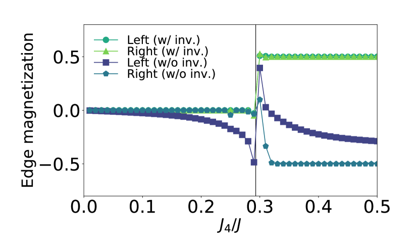
Figure 8: Comparison of edge magnaetizations $M_{\rm right}^{z}$ and $M_{\rm left}^{z}$ for $L=242$ (circles and triangles) and for $L=240$ (squares and pentagons). The other parameters are fixed to $h_{u}/J=1.5$ and $\alpha=0.2$. The former case has the $I_{b}$ symmetry and the latter has not. The inversion symmetry quantizes the edge magnetizations except in the vicinity of the quantum critical point $J_{4}/J=0.295$. Without the inversion symmetry, the edge magnetization shows continuous changes even away from the quantum critical point.

Despite the quantum critical behaviors of the excitation gap and the entanglement entropy, the order parameters show discontinuous behaviors because of the inversion symmetry. Figure 8 shows the edge magnetizations with and without the $\mathcal{I}_{b}$ symmetry. The $\mathcal{I}_{b}$ symmetry imposes a strong constraint on the edge magnetization as the bulk polarization. Recall that $U$ is given by Eq. (50). The exact $\mathcal{I}_{b}$ symmetry of the model (55) leads to

$$\braket{U} =\braket{\mathcal{I}_{b}U\mathcal{I}_{b}^{-1}}$$

$$=\biggl{\langle}\exp\biggl{(}i\frac{2\pi}{L}\sum_{j=1}^{L}jC_{L+1-j}\biggr{)}\biggr{\rangle}$$

$$=\biggl{\langle}\exp\biggl{(}i\frac{2\pi}{L}\sum_{j=1}^{L}(L+1-j)C_{j}\biggr{)}\biggr{\rangle}$$

$$=\braket{U^{\dagger}}\exp\biggl{(}2\pi i\biggl{(}1+\frac{1}{L}\biggr{)}\sum_{j=1}^{L}\braket{C_{j}^{z}}\biggr{)}$$ (215)

The charge neutrality condition, $\sum_{j=1}^{L}\braket{C_{j}}=0$, leads to $\braket{U}=\braket{U^{\dagger}}$. Accordingly, if $\braket{U}\not=0$,

$$\mathcal{P} =\frac{1}{2\pi}\operatorname{Im}\ln\braket{U}=0\text{ or }\frac{1}{2}\mod 1.$$ (216)

The condition $\braket{U}\not=0$ is equivalent to the locking of $\phi$. $\braket{U}=0$ holds at the quantum critical point where the $\phi$ field is gapless, where the edge polarization is ill-defined.

In the absence of the $\mathcal{I}_{b}$ symmetry, the edge magnetization is not necessarily quantized. Indeed, Fig. 8 shows that $M_{\rm left}^{z}$ depends on $J_{4}$ continuously except for the quantum critical point $J_{4}=J_{4c}$. By contrast, the other edge $M_{\rm right}^{z}$ is well quantized. This asymmetric behavior of the quantization can be understood as the modification of the boundary condition. The spin chain (55) has the exact $\mathcal{I}_{b}$ symmetry with the OBC for $L=2\mod 4$. By adding two sites to one edge of the chain, say, the left edge, we can make $L=0\mod 4$ and violate the $\mathcal{I}_{b}$ symmetry. We can expect that such addition of sites hardly modifies the bulk Hamiltonian and generate a symmetry-breaking potential localized at the left edge of the chain. The most relevant interaction is the staggered magnetic field, $h_{B}\sin(2\phi(0,\tau))$. This boundary staggered field alters the boundary condition on the left edge from $\phi(x=0)=0$ to

$$\phi(x=0,\tau)=\Phi,$$ (217)

with a constant $\Phi$. This modification of the boundary condition explains the continuous change of the edge magnetization (Fig. 8) in the absence of the $\mathcal{I}_{b}$ symmetry.

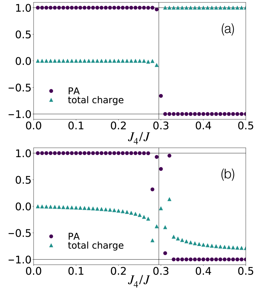
Figure 9: $J_{4}$ dependence of polarization amplitude $\braket{U}$ (circles) and total charge $\sum_{j=1}^{L}\braket{C_{j}}$ (triangles) for $h_{u}/J=1.5$, $\alpha=0.2$ with system size (a) $L=242$ and (b) $L=240$. (a) When the $\mathcal{I}_{b}$ symmetry is present, the polarization amplitude and the total charge show abrupt changes at $J_{4}/J\approx 0.295$ thanks to the $\mathcal{I}_{b}$ symmetry. (b) On the other hand, when the $\mathcal{I}_{b}$ symmetry is absent, the total charge changes continuously though the accuracy of the numerical data is extremely lowered in the vicinity of the quantum critical point $J_{4}/J\approx 0.295$. Note that apart from $\braket{U}$ and the total charge, the other thermodynamic quantities behave similarly regardless of the presence of the absence of the $\mathcal{I}_{b}$ symmetry.

The edge magnetization as the bulk polarization (216) works as an order parameter to distinguish the $\bar{\phi}=0$ phase ($\mathcal{P}=0$) and the $\bar{\phi}=\pi/2$ phase ($\mathcal{P}=1/2\mod 1$). Likewise, the polarization amplitude $\braket{U}$ can also be regarded as the order parameter. Figure 9 shows the $J_{4}$ dependence of the polarization amplitude $\braket{U}$ and the total charge, $\sum_{j=1}^{L}\braket{C_{j}}$. The abrupt jump of the order parameter (216) is due to the $\mathcal{I}_{b}$ symmetry. The polarization amplitude $\braket{U}$ also jumps unlike the bond-alternating spin-$S$ chains at zero magnetic fields Nakamura and Todo (2002), though the polarization amplitude is not necessarily quantized as $\braket{U}=\pm 1$. If the excitation gap closes at the transition point, the polarization amplitude will change continuously and cross zero at the transition point. Therefore, the observed jump of Fig. 9 implies that the quantum critical regime is too narrow to observe such a continuous change of $\braket{U}$.

The total charge can also be seen as an order parameter to distinguish the two phases of concern [Fig. 9 (a)]. The charge neutrality is weakly broken for $J_{4}>J_{4c}$. Nevertheless, since the discrepancy of the charge is precisely one, the quantum phase remains on the $1/2$ magnetization plateau in the $L\to+\infty$ limit, $M/M_{s}=\frac{1}{2}+\frac{1}{L}\to\frac{1}{2}$.

The $J_{4}$ dependence of the total charge becomes continuous in the absence of the $\mathcal{I}_{b}$ symmetry [Fig. 9 (b)]. Besides, the total charge tends to $-1$ in the $J_{4}/J$ limit. The sign change compared to the $I_{b}$-symmetric case remains obscure at this stage. Except for this continuous decrease of the total charge, the numerical results and the field-theoretical analyses are consistent.

Appendix E Union-jack strip

The effective field theory (68) of the union-jack strip

$$\mathcal{H}_{\rm UJ} =J_{1}\sum_{j=1}^{L}\sum_{n=1}^{3}\bm{S}_{j,n}\cdot\bm{S}_{j+1,n}+J_{1}\sum_{j=1}^{L}\bm{S}_{j,2}\cdot(\bm{S}_{j,1}+\bm{S}_{j,3})$$

$$+J_{2}\sum_{j=2}^{L-1}\bm{S}_{j,2}\cdot(\bm{S}_{j-1,1}+\bm{S}_{j-1,3}+\bm{S}_{j+1,1}+\bm{S}_{j+1,3})$$

$$-h_{u}\sum_{j=1}^{L}\sum_{n=1}^{3}S_{j,n}^{z},$$ (218)

on the $1/3$ plateau is derived similarly to that in Appendix C. The infinitesimal uniform magnetic field $h_{u}>0$ is imposed to break the $S^{z}\to-S^{z}$ symmetry. We consider the classical configuration,

$$\bm{\Omega}_{n}(x_{j},\tau) =\begin{pmatrix}(-1)^{j+n}\sqrt{1-(m/S)^{2}}\cos\theta_{n}(x_{j},\tau)\\ (-1)^{j+n}\sqrt{1-(m/S)^{2}}\sin\theta_{n}(x_{j},\tau)\\ m/S\end{pmatrix},$$ (219)

for each leg. The index $n=1,2,3$ denotes the $n$th leg. The interleg interaction leads to

$$\theta_{1}(x,\tau) =\theta_{2}(x,\tau)=\theta_{3}(x,\tau),$$ (220)

modulo $2\pi$ in the ground state. The Berry phase is thus given by

$$\mathcal{S}_{\rm BP} =3\pi i(S-m)Q_{\rm v}-3i(S-m)\int_{0}^{L}\frac{dx}{a_{0}}\int_{0}^{\beta}d\tau\,\partial_{\tau}\theta(x,\tau),$$ (221)

where $\theta=(\theta_{1}+\theta_{2}+\theta_{3})/3$. Since $3(S-m)=1$ for the spin-$1/2$ union-jack strip on the $1/3$ plateau, the dual theory is derived similarly to Appendix C.3.1.

$$\mathcal{S}_{\rm dual} =\frac{v}{2\pi K}\int d\tau dx\,(\partial_{\mu}\phi)^{2}$$

$$\qquad-2\zeta\cos[3\pi(S-m)]\int d\tau dx\,\cos(2\phi),$$ (222)

with $\phi=\phi_{1}+\phi_{2}+\phi_{3}$. In this formulation, the long-range antiferromagnetic order results from the locking of $\phi$. The semiclassical bosonization formulas on the $1/3$ plateau differ from Eqs. (184) and (185) because the staggered magnetic field,

$$h_{s}\sum_{j=1}^{L}\sum_{n=1}^{3}(-1)^{j+n}S_{j,n}^{z},$$ (223)

keeps all the symmetries of the model (218). This symmetry implies the bosonization formula,

$$(-1)^{j+n}S_{j,n}^{z}\propto\cos(2\phi).$$ (224)

References

- Landau et al. (2013) L. D. Landau, E. M. Lifshitz, and L. P. Pitaevski, Electrodynamics of continuous media, Vol. 8 (Butterworth-Heinemann, Oxford, 2013).
- Vanderbilt and King-Smith (1993) David Vanderbilt and R. D. King-Smith, “Electric polarization as a bulk quantity and its relation to surface charge,” Phys. Rev. B 48, 4442–4455 (1993).
- Benalcazar et al. (2017a) Wladimir A. Benalcazar, B. Andrei Bernevig, and Taylor L. Hughes, “Electric multipole moments, topological multipole moment pumping, and chiral hinge states in crystalline insulators,” Phys. Rev. B 96, 245115 (2017a).
- Benalcazar et al. (2017b) Wladimir A. Benalcazar, B. Andrei Bernevig, and Taylor L. Hughes, “Quantized electric multipole insulators,” Science 357, 61–66 (2017b).
- Qi et al. (2008) Xiao-Liang Qi, Taylor L. Hughes, and Shou-Cheng Zhang, “Topological field theory of time-reversal invariant insulators,” Phys. Rev. B 78, 195424 (2008).
- Ezawa (2018) Motohiko Ezawa, “Higher-Order Topological Insulators and Semimetals on the Breathing Kagome and Pyrochlore Lattices,” Phys. Rev. Lett. 120, 026801 (2018).
- Pollmann et al. (2010) Frank Pollmann, Ari M. Turner, Erez Berg, and Masaki Oshikawa, “Entanglement spectrum of a topological phase in one dimension,” Phys. Rev. B 81, 064439 (2010).
- Pollmann et al. (2012) Frank Pollmann, Erez Berg, Ari M. Turner, and Masaki Oshikawa, “Symmetry protection of topological phases in one-dimensional quantum spin systems,” Phys. Rev. B 85, 075125 (2012).
- Affleck et al. (1988) Ian Affleck, Tom Kennedy, Elliott H. Lieb, and Hal Tasaki, “Valence bond ground states in isotropic quantum antiferromagnets,” Communications in Mathematical Physics 115, 477–528 (1988).
- Kennedy and Tasaki (1992) Tom Kennedy and Hal Tasaki, “Hidden zz2 symmetry breaking in haldane-gap antiferromagnets,” Phys. Rev. B 45, 304–307 (1992).
- Kohmoto and Tasaki (1992) Mahito Kohmoto and Hal Tasaki, “Hidden zz2symmetry breaking and the haldane phase in the s=1/2 quantum spin chain with bond alternation,” Phys. Rev. B 46, 3486–3495 (1992).
- Nakamura and Todo (2002) Masaaki Nakamura and Synge Todo, “Order Parameter to Characterize Valence-Bond-Solid States in Quantum Spin Chains,” Phys. Rev. Lett. 89, 077204 (2002).
- Watanabe et al. (2021) Haruki Watanabe, Yasuyuki Kato, Hoi Chun Po, and Yukitoshi Motome, “Fractional corner magnetization of collinear antiferromagnets,” Phys. Rev. B 103, 134430 (2021).
- Kane et al. (2002) C. L. Kane, Ranjan Mukhopadhyay, and T. C. Lubensky, “Fractional quantum hall effect in an array of quantum wires,” Phys. Rev. Lett. 88, 036401 (2002).
- Teo and Kane (2014) Jeffrey C. Y. Teo and C. L. Kane, “From luttinger liquid to non-abelian quantum hall states,” Phys. Rev. B 89, 085101 (2014).
- Meng et al. (2015) Tobias Meng, Titus Neupert, Martin Greiter, and Ronny Thomale, “Coupled-wire construction of chiral spin liquids,” Phys. Rev. B 91, 241106 (2015).
- Lecheminant and Tsvelik (2017) P. Lecheminant and A. M. Tsvelik, “Lattice spin models for non-abelian chiral spin liquids,” Phys. Rev. B 95, 140406 (2017).
- Marshall (1955) W. Marshall, “Antiferromagnetism,” Proceedings of the Royal Society of London. Series A. Mathematical and Physical Sciences 232, 48–68 (1955).
- Lieb and Mattis (1962) Elliott Lieb and Daniel Mattis, “Ordering energy levels of interacting spin systems,” Journal of Mathematical Physics 3, 749–751 (1962).
- Giamarchi (2004) T. Giamarchi, Quantum Physics in One Dimension (Oxford University Press, Oxford, 2004).
- Gogolin et al. (2004) Alexander O Gogolin, Alexander A Nersesyan, and Alexei M Tsvelik, Bosonization and strongly correlated systems (Cambridge university press, 2004).
- Hikihara and Furusaki (2004) T. Hikihara and A. Furusaki, “Correlation amplitudes for the spin- chain in a magnetic field,” Phys. Rev. B 69, 064427 (2004).
- Resta (1998) Raffaele Resta, “Quantum-Mechanical Position Operator in Extended Systems,” Phys. Rev. Lett. 80, 1800–1803 (1998).
- Watanabe and Oshikawa (2018) Haruki Watanabe and Masaki Oshikawa, “Inequivalent Berry Phases for the Bulk Polarization,” Phys. Rev. X 8, 021065 (2018).
- Lieb et al. (1961) Elliott Lieb, Theodore Schultz, and Daniel Mattis, “Two soluble models of an antiferromagnetic chain,” Annals of Physics 16, 407 – 466 (1961).
- Oshikawa (2000) Masaki Oshikawa, “Commensurability, Excitation Gap, and Topology in Quantum Many-Particle Systems on a Periodic Lattice,” Phys. Rev. Lett. 84, 1535–1538 (2000).
- Oshikawa et al. (1997) Masaki Oshikawa, Masanori Yamanaka, and Ian Affleck, “Magnetization Plateaus in Spin Chains: “Haldane Gap” for Half-Integer Spins,” Phys. Rev. Lett. 78, 1984–1987 (1997).
- Yao and Oshikawa (2020) Yuan Yao and Masaki Oshikawa, “Generalized Boundary Condition Applied to Lieb-Schultz-Mattis-Type Ingappabilities and Many-Body Chern Numbers,” Phys. Rev. X 10, 031008 (2020).
- Cho et al. (2017) Gil Young Cho, Chang-Tse Hsieh, and Shinsei Ryu, “Anomaly manifestation of Lieb-Schultz-Mattis theorem and topological phases,” Phys. Rev. B 96, 195105 (2017).
- Furuya and Oshikawa (2017) Shunsuke C. Furuya and Masaki Oshikawa, “Symmetry Protection of Critical Phases and a Global Anomaly in Dimensions,” Phys. Rev. Lett. 118, 021601 (2017).
- Yao et al. (2019) Yuan Yao, Chang-Tse Hsieh, and Masaki Oshikawa, “Anomaly Matching and Symmetry-Protected Critical Phases in Spin Systems in Dimensions,” Phys. Rev. Lett. 123, 180201 (2019).
- Kobayashi et al. (2018) Ryohei Kobayashi, Yuya O. Nakagawa, Yoshiki Fukusumi, and Masaki Oshikawa, “Scaling of the polarization amplitude in quantum many-body systems in one dimension,” Phys. Rev. B 97, 165133 (2018).
- Nakamura and Furuya (2019) Masaaki Nakamura and Shunsuke C. Furuya, “Extraction of topological information in Tomonaga-Luttinger liquids,” Phys. Rev. B 99, 075128 (2019).
- Furuya and Nakamura (2019) Shunsuke C. Furuya and Masaaki Nakamura, “Polarization amplitude near quantum critical points,” Phys. Rev. B 99, 144426 (2019).
- Eggert and Affleck (1992) Sebastian Eggert and Ian Affleck, “Magnetic impurities in half-integer-spin heisenberg antiferromagnetic chains,” Phys. Rev. B 46, 10866–10883 (1992).
- Schulz (1986) H. J. Schulz, “Phase diagrams and correlation exponents for quantum spin chains of arbitrary spin quantum number,” Phys. Rev. B 34, 6372–6385 (1986).
- Kim et al. (2000) Eugene H. Kim, G. Fáth, J. Sólyom, and D. J. Scalapino, “Phase transitions between topologically distinct gapped phases in isotropic spin ladders,” Phys. Rev. B 62, 14965–14974 (2000).
- Hijii et al. (2005) Keigo Hijii, Atsuhiro Kitazawa, and Kiyohide Nomura, “Phase diagram of two-leg spin-ladder systems,” Phys. Rev. B 72, 014449 (2005).
- Shelton et al. (1996) D. G. Shelton, A. A. Nersesyan, and A. M. Tsvelik, “Antiferromagnetic spin ladders: Crossover between spin S=1/2 and S=1 chains,” Phys. Rev. B 53, 8521–8532 (1996).
- Chitra and Giamarchi (1997) R. Chitra and T. Giamarchi, “Critical properties of gapped spin-chains and ladders in a magnetic field,” Phys. Rev. B 55, 5816–5826 (1997).
- Lecheminant and Orignac (2002) P. Lecheminant and E. Orignac, “Magnetization and dimerization profiles of the cut two-leg spin ladder,” Phys. Rev. B 65, 174406 (2002).
- Orignac and Lecheminant (2003) E. Orignac and P. Lecheminant, “Magnetization and dimerization profiles of open spin ladders,” Physica B: Condensed Matter 329-333, 971–972 (2003).
- Robinson et al. (2019) Neil J. Robinson, Alexander Altland, Reinhold Egger, Niklas M. Gergs, Wei Li, Dirk Schuricht, Alexei M. Tsvelik, Andreas Weichselbaum, and Robert M. Konik, “Nontopological majorana zero modes in inhomogeneous spin ladders,” Phys. Rev. Lett. 122, 027201 (2019).
- Fuji (2016) Yohei Fuji, “Effective field theory for one-dimensional valence-bond-solid phases and their symmetry protection,” Phys. Rev. B 93, 104425 (2016).
- Affleck (1989) I Affleck, “Quantum spin chains and the Haldane gap,” Journal of Physics: Condensed Matter 1, 3047–3072 (1989).
- Sachdev (2007) Subir Sachdev, Quantum phase transitions (Cambridge University Press, Cambridge, 2007).
- Auerbach (1998) Assa Auerbach, Interacting electrons and quantum magnetism (Springer-Verlag, New York, 1998).
- Affleck (1986) Ian Affleck, “Mass generation by merons in quantum spin chains and the O(3) model,” Phys. Rev. Lett. 56, 408–411 (1986).
- Gross (1978) David J. Gross, “Meron configurations in the two-dimensional O(3) -model,” Nuclear Physics B 132, 439–456 (1978).
- Kosterlitz and Thouless (1973) J M Kosterlitz and D J Thouless, “Ordering, metastability and phase transitions in two-dimensional systems,” Journal of Physics C: Solid State Physics 6, 1181–1203 (1973).
- Kosterlitz (1974) J M Kosterlitz, “The critical properties of the two-dimensional xy model,” Journal of Physics C: Solid State Physics 7, 1046–1060 (1974).
- Tonegawa et al. (2011) Takashi Tonegawa, Kiyomi Okamoto, Hiroki Nakano, Tôru Sakai, Kiyohide Nomura, and Makoto Kaburagi, “Haldane, Large-, and Intermediate- in Quantum Spin Chain with On-Site and XXZ Anisotropies,” Journal of the Physical Society of Japan 80, 043001 (2011).
- Shindou (2005) Ryuichi Shindou, “Quantum Spin Pump in S=1/2 Antiferromagnetic Chains –Holonomy of Phase Operators in sine-Gordon Theory–,” Journal of the Physical Society of Japan 74, 1214–1223 (2005).
- Fuji et al. (2015) Yohei Fuji, Frank Pollmann, and Masaki Oshikawa, “Distinct Trivial Phases Protected by a Point-Group Symmetry in Quantum Spin Chains,” Phys. Rev. Lett. 114, 177204 (2015).
- Schulz (1980) H. J. Schulz, “Critical behavior of commensurate-incommensurate phase transitions in two dimensions,” Phys. Rev. B 22, 5274–5277 (1980).
- Fishman et al. (2020) Matthew Fishman, Steven R. White, and E. Miles Stoudenmire, “The ITensor Software Library for Tensor Network Calculations,” (2020), arXiv:2007.14822 .
- Tonegawa et al. (1998) Takashi Tonegawa, Takeshi Nishida, and Makoto Kaburagi, “Ground-state magnetization curve of a generalized spin-1/2 ladder,” Physica B: Condensed Matter 246-247, 368–371 (1998).
- Giamarchi and Tsvelik (1999) T. Giamarchi and A. M. Tsvelik, “Coupled ladders in a magnetic field,” Phys. Rev. B 59, 11398–11407 (1999).
- Bouillot et al. (2011) Pierre Bouillot, Corinna Kollath, Andreas M. Läuchli, Mikhail Zvonarev, Benedikt Thielemann, Christian Rüegg, Edmond Orignac, Roberta Citro, Martin Klanjšek, Claude Berthier, Mladen Horvatić, and Thierry Giamarchi, “Statics and dynamics of weakly coupled antiferromagnetic spin- ladders in a magnetic field,” Phys. Rev. B 83, 054407 (2011).
- Narumi et al. (2004) Yasuo Narumi, Koichi Kindo, Masayuki Hagiwara, Hiroki Nakano, Akira Kawaguchi, Kouichi Okunishi, and Masanori Kohno, “High-field magnetization of antiferromagnetic bond-alternating chain compounds,” Phys. Rev. B 69, 174405 (2004).
- Okamoto et al. (2001) Kiyomi Okamoto, Nobuhisa Okazaki, and Tôru Sakai, “Magnetization plateau of frustrated spin ladder,” Journal of the Physical Society of Japan 70, 636–639 (2001).
- Totsuka (1997) Keisuke Totsuka, “Magnetization processes in bond-alternating quantum spin chains,” Physics Letters A 228, 103–110 (1997).
- Tanaka et al. (2009) Akihiro Tanaka, Keisuke Totsuka, and Xiao Hu, “Geometric phases and the magnetization process in quantum antiferromagnets,” Phys. Rev. B 79, 064412 (2009).
- Takayoshi et al. (2015) Shintaro Takayoshi, Keisuke Totsuka, and Akihiro Tanaka, “Symmetry-protected topological order in magnetization plateau states of quantum spin chains,” Phys. Rev. B 91, 155136 (2015).
- Takahashi and Sakai (1991) Minoru Takahashi and Tôru Sakai, “Magnetization Curve and Correlation Function of Haldane-Gap Antiferromagnet in Strong Magnetic Field,” Journal of the Physical Society of Japan 60, 760–763 (1991).
- Calabrese and Cardy (2004) Pasquale Calabrese and John Cardy, “Entanglement entropy and quantum field theory,” Journal of Statistical Mechanics: Theory and Experiment 2004, P06002 (2004).
- Shimokawa and Nakano (2013) Tokuro Shimokawa and Hiroki Nakano, “Nontrivial ferrimagnetism of the heisenberg model on the union jack strip lattice,” Journal of the Korean Physical Society 63, 591–595 (2013).
- Furuya and Giamarchi (2014) Shunsuke C. Furuya and Thierry Giamarchi, “Spontaneously magnetized tomonaga-luttinger liquid in frustrated quantum antiferromagnets,” Phys. Rev. B 89, 205131 (2014).
- Takayoshi et al. (2014) Shintaro Takayoshi, Masahiro Sato, and Takashi Oka, “Laser-induced magnetization curve,” Phys. Rev. B 90, 214413 (2014).
- Sakai and Takahashi (1998) Tôru Sakai and Minoru Takahashi, “Magnetization plateau in an antiferromagnetic Heisenberg chain with anisotropy,” Phys. Rev. B 57, R3201–R3204 (1998).
- Kitazawa and Okamoto (2000) Atsuhiro Kitazawa and Kiyomi Okamoto, “Magnetization-plateau state of the spin chain with single-ion anisotropy,” Phys. Rev. B 62, 940–945 (2000).
- Furuya and Oshikawa (2012) Shunsuke C. Furuya and Masaki Oshikawa, “Boundary Resonances in Antiferromagnetic Chains Under a Staggered Field,” Phys. Rev. Lett. 109, 247603 (2012).
- Sénéchal (1995) D. Sénéchal, “Semiclassical description of spin ladders,” Phys. Rev. B 52, 15319–15326 (1995).
- Sierra (1996) Germán Sierra, “The nonlinear sigma model and spin ladders,” Journal of Physics A: Mathematical and General 29, 3299–3310 (1996).
- Dell’Aringa et al. (1997) S. Dell’Aringa, E. Ercolessi, G. Morandi, P. Pieri, and M. Roncaglia, “Effective actions for spin ladders,” Phys. Rev. Lett. 78, 2457–2460 (1997).
- Sato and Oshikawa (2007) Masahiro Sato and Masaki Oshikawa, “Magnon bands of -leg integer-spin antiferromagnetic systems in the weak-interchain-coupling regime,” Phys. Rev. B 75, 014404 (2007).
- Haldane (1983a) F. D. M. Haldane, “Continuum dynamics of the 1-D Heisenberg antiferromagnet: Identification with the O(3) nonlinear sigma model,” Physics Letters A 93, 464–468 (1983a).
- Haldane (1983b) F. D. M. Haldane, “Nonlinear Field Theory of Large-Spin Heisenberg Antiferromagnets: Semiclassically Quantized Solitons of the One-Dimensional Easy-Axis Néel State,” Phys. Rev. Lett. 50, 1153–1156 (1983b).
- Chen et al. (2003) Wei Chen, Kazuo Hida, and B. C. Sanctuary, “Ground-state phase diagram of chains with uniaxial single-ion-type anisotropy,” Phys. Rev. B 67, 104401 (2003).
- Nagaosa and Tokura (2013) Naoto Nagaosa and Yoshinori Tokura, “Topological properties and dynamics of magnetic skyrmions,” Nature Nanotechnology 8, 899–911 (2013).
- Di Francesco et al. (1998) Philippe Di Francesco, Pierre Mathieu, and David Sénéchal, Conformal field theory (Springer-Verlag, New York, 1998).
- Orignac (2004) E. Orignac, “Quantitative expression of the spin gap via bosonization for a dimerized spin-1/2 chain,” The European Physical Journal B 39, 335–339 (2004).
- Takayoshi and Sato (2010) Shintaro Takayoshi and Masahiro Sato, “Coefficients of bosonized dimer operators in spin- chains and their applications,” Phys. Rev. B 82, 214420 (2010).
- Hikihara et al. (2017) Toshiya Hikihara, Akira Furusaki, and Sergei Lukyanov, “Dimer correlation amplitudes and dimer excitation gap in spin- xxz and heisenberg chains,” Phys. Rev. B 96, 134429 (2017).
- Berg et al. (2008) Erez Berg, Emanuele G. Dalla Torre, Thierry Giamarchi, and Ehud Altman, “Rise and fall of hidden string order of lattice bosons,” Phys. Rev. B 77, 245119 (2008).
- Lamas et al. (2011) C. A. Lamas, S. Capponi, and P. Pujol, “Combined analytical and numerical approach to study magnetization plateaux in doped quasi-one-dimensional antiferromagnets,” Phys. Rev. B 84, 115125 (2011).
- Furuya (2020) Shunsuke C. Furuya, “Field-induced dimer orders in quantum spin chains,” Phys. Rev. B 101, 134425 (2020).