Superradiance in dynamically modulated Tavis-Cummings model with spectral disorder

Abstract

Superradiance is the enhanced emission of photons from quantum emitters collectively coupling to the same optical mode. However, disorder in the resonant frequencies of the quantum emitters can perturb this effect. In this paper, we study the interplay between superradiance and spectral disorder in a dynamically modulated Tavis-Cummings model. Through numerical simulations and analytical calculations, we show that the effective cooperativity of the superradiant mode, which is always formed over an extensive number of emitters, can be multiplicatively enhanced with a quantum control protocol modulating the resonant frequency of the optical mode. Our results are relevant to experimental demonstration of superradiant effects in solid-state quantum optical systems, wherein the spectral disorder is a significant technological impediment towards achieving photon-mediated emitter-emitter couplings.

Coherent interaction between a collection of quantum emitters and an optical mode, theoretically described by the Tavis-Cummings model Tavis and Cummings (1968), has been a topic of intense theoretical interest since the conception of quantum optics. Multiple emitters coupling strongly to the same optical mode are known to exhibit cooperative effects, the most prominent of which is the formation of a superradiant state Gross and Haroche (1982); Rehler and Eberly (1971); Scully and Svidzinsky (2009); Dicke (1954). Superradiant states are fully symmetric collective excitations of the multiple emitters whose interaction with the optical mode is enhanced due to a constructive interference of the individually emitted photons. These states underlie the physical phenomena of collective spontaneous emission (Dicke superradiance) Dicke (1954); Andreev et al. (1980); Clemens et al. (2003); Eleuch and Rotter (2014) and superradiant phase transitions Hepp and Lieb (1973); Lambert et al. (2004); Bamba et al. (2016). Furthermore, the enhancement of light-matter interaction in such systems has implications for design and implementation of a number of quantum information processing blocks, such as transducers Casabone et al. (2015), memories Ortiz-Gutiérrez et al. (2018) and non-classical light sources Jahnke et al. (2016).

However, technologically relevant experimental systems that can potentially demonstrate and use superradiance, such as solid-state quantum optical systems like quantum dots Scheibner et al. (2007); Grim et al. (2019), color centers Angerer et al. (2018) and rare-earth ions Zhong et al. (2017), often suffer from spectral disorder amongst the quantum emitters. Since spectral disorder can disrupt interactions between emitters, it competes with the collective emitter-optical mode interaction and can prevent the formation of the superradiant state. This interplay between disorder and coherent interaction has been extensively studied in time-independent quantum systems arising in many-body physics Anderson (1958); Lee and Fisher (1981); Alet and Laflorencie (2018); Nandkishore and Huse (2015); Pal and Huse (2010); Nandkishore and Sondhi (2017); Nag and Garg (2019); Smith et al. (2016) as well as quantum optics Moreira et al. (2019); Akkermans et al. (2008); Ashhab and Semba (2017); Biella et al. (2013); Cottier et al. (2018); Kelly et al. (2021); Manzoni et al. (2017); Fayard et al. (2021); Temnov and Woggon (2005); Trivedi et al. (2019); Mivehvar et al. (2017); Debnath et al. (2019) There has been recent interest in understanding the impact of dynamical modulation, applied globally on all the emitters, on the properties of such models. Such modulation schemes are easily experimentally accessible, e.g. in quantum optical systems with a dynamically modulated optical mode (such as modulation of the resonant frequency of a cavity Zhang et al. (2019)) or with collectively modulated emitters (through simultaneously laser driving or stark shifting the resonant frequencies of all emitters Sun et al. (2018); Lukin et al. (2020)). These global quantum controls designed with off-the-shelf optimization techniques De Fouquieres et al. (2011); d’Alessandro (2007) have been be used to potentially compensate for, or in some cases exploit, the spectral disorder Julsgaard et al. (2013); Gorshkov et al. (2008) for building quantum information processing hardware such as quantum transducers and memories. However, an understanding of their effectiveness in compensating disorder, specially in the thermodynamic limit of large number of emitters, is less well understood.

In this paper, we study the interplay of superradiance and spectral disorder in a dynamically modulated Tavis-Cummings model. Within the single-photon subspace, the all-to-all coupling between the emitters enables the formation of a superradiant state over an extensive number of emitters irrespective of the extent of disorder in the system. We study the impact of the dynamical modulation, designed as a quantum control to compensate for the spectral disorder in the system, on the formation of this superradiant state. We demonstrate that this dynamical modulation can achieve a multiplicative enhancement in the cooperativity of the superradiant state even in the limit of a large number of emitters. Finally, we provide evidence that this control pulse, designed by only considering single-photon dynamics, also multiplicatively enhances superradiance in the multi-photon subspaces of the Tavis-Cummings model.

We consider $N$ emitters coupled to a cavity with the following Hamiltonian (Fig 1a)

$$H=\omega_{c}(t)a^{\dagger}a+H_{e}+H_{c},\ \text{where}$$

$$H_{e}=\sum_{i=1}^{N}\omega_{i}\sigma_{i}^{\dagger}\sigma_{i}\text{ and }H_{c}=g(N)\sum_{i=1}^{N}(a^{\dagger}\sigma_{i}+\sigma_{i}^{\dagger}a)$$ (1)

where $\omega_{c}(t)$ is the time dependent frequency of the cavity, $\omega_{i}$ is the resonant frequency of the $i$th emitter, $a^{\dagger}$ is the raising operator of the cavity, $\sigma_{i}^{\dagger}$ is the excitation operator of the $i$th emitter, and $g(N)$ is the emitter-cavity coupling strength (which we allow to depend on the number of emitters). Furthermore, we assume that the cavity emits into an output channel with decay rate $\kappa$, and the emitters in addition to coupling to the cavity also individually decay with decay rate $\gamma$. We will denote the ground state of this model, with no photons in the cavity and all emitters in their individual ground state, by $\ket{\text{G}}$.

To quantify the superradiant behavior of this system, we use two metrics: eigenstate superradiance and photon generation fidelity. The eigenstate superradiance (ES) is calculated as

$$\mu_{\text{ES}}[\omega_{c}(t)]=\max_{\ket{\phi}}\bigg{|}\bra{\text{G}}\sum_{i=1}^{N}\sigma_{i}\ket{\phi}\bigg{|}^{2},$$ (2)

where the maximization is done over all $\ket{\phi}$, the single-photon Floquet eigenstates of $H(t)$. This metric can be interpreted as a measure of the coupling between the (most) superradiant state and the ground state $\ket{\text{G}}$ induced by $H_{c}$. We point out that in the absence of disorder and with the emitters being on-resonance with the cavity mode, $\mu_{\text{ES}}=N/2$. Additionally, we calculate the photon generation fidelity; we initialize the emitters to an initial symmetric state (i.e. $\sum_{i=1}^{N}\sigma_{i}^{\dagger}\ket{\text{G}}/\sqrt{N}$), allow it to decay into the output channel through the cavity, and compute the probability of a photon being emitted into the output channel:

$$\mu_{\text{FID}}[\omega_{c}(t)]=\kappa\int_{0}^{\infty}\langle a^{\dagger}(t)a(t)\rangle dt.$$ (3)

We begin by studying the behavior of an unmodulated system ($\omega_{c}(t)=0$) within the single photon subspace as a function of $N$. Fig. 1b considers a setting where the coupling strength between the cavity and emitters is independent of $N$ (i.e. $g(N)\sim$ constant) – in this case within the single-photon subspace, $\left\|{H_{c}}\right\|\sim g(N)\sqrt{N}\sim\sqrt{N}$ and $\left\|{H_{e}}\right\|\sim\text{constant}$. Hence, for large $N$ the dynamics of this system is completely dominated by $H_{c}$ and spectral disorder does not play any role. This is evidenced both by the eigenvalue superradiance approaching $N/2$ as $N\to\infty$ and the single-photon generation fidelity approaching the fidelity of the homogeneous system (Fig. 1b). A more interesting setting, studied in Fig. 1c, is where $g(N)\sim 1/\sqrt{N}$ so as to make the norms $\left\|{H_{c}}\right\|$ and $\left\|{H_{e}}\right\|$ comparable at large $N$. In this case, while superradiance is not completely recovered as $N\to\infty$, we find that the eigenstate superradiance still scales as $N$ — consequently, a superradiant state is still formed between an extensive number (but not all) of emitters. Likewise, the single photon generation fidelity approaches a non-zero constant as $N\rightarrow\infty$ — since the coupling constant vanishes in this limit, this is only possible if an extensive number of emitters are cooperatively emitting into the cavity mode. The formation of a superradiant state over an extensive number of emitters stems from the all-to-all coupling between the emitters mediated by the cavity mode, making it fundamentally different from the impact of disorder in models with local interactions, wherein the number of emitters cooperatively interacting with each other would grow at most logarithmically with $N$ Anderson (1958); Aizenman and Molchanov (1993).

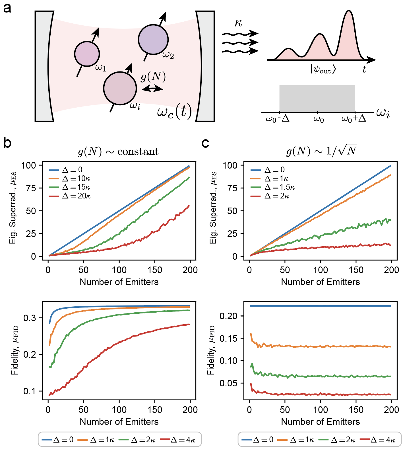
Figure 1: Setup and Unmodulated System Scaling (a) We consider $N$ emitters with frequencies $\omega_{i}$ coupled to a cavity with rate $g(N)$. The cavity is driven by a pulse that imparts a frequency shift $\omega_{c}(t)$ and is coupled to a waveguide with rate $\kappa$. (b) Single photon eigenstate superradiance and fidelity of the unmodulated ($\omega_{c}(t)=0$) system in (a), with coupling strength $g=\kappa$ held constant. Single photon emission fidelity is calculated in the presence of external decay at rate $2\kappa$. (c) Eigenstate superradiance and fidelity with $g$ scaled as $g=\kappa/\sqrt{N}$. All plots show the average value from 25 different emitter ensembles with frequencies sampled from a uniform distribution.

Figure 2: Pulse Optimization (a) Output photon flux before and after optimization for $N=10,50,$ and $150$ with $g=\kappa/\sqrt{N}$, $\Delta=10\kappa$, and constant external decay rate $0.5\kappa$. Transparent lines show the photon flux for each ensemble and solid lines show the average. (b) Optimized single photon emission fidelity scaling with $N$ for $g=\kappa/\sqrt{N}$, $\Delta=10\kappa$, and constant external decay rate $0.5\kappa$. (c) Optimized eigenstate superradiance scaling with $N$ for $g=\kappa/\sqrt{N}$ and $\Delta=10\kappa$. With these parameters a homogeneous ensemble would exhibit an eigenstate superradiance of $N/2$. Plots show the average value from 25 different emitter ensembles.

We next consider the impact of dynamical modulation of cavity resonance $\omega_{c}(t)$ on superradiance. To find a modulation signal that best compensates for the spectral disorder, we maximize the single photon generation fidelity (Eq. 3) with respect to $\omega_{c}(t)$. The optimized modulation signal is computed by using time-dependent scattering theory Trivedi et al. (2018); Fischer et al. (2018) together with adjoint-sensitivity analysis Cao et al. (2003) (see supplementary for details) to solve the maximization problem. Figure 2a shows the impact that applying this modulation has on the photon emission rate ($\kappa\langle a^{\dagger}(t)a(t)\rangle$) into the output channel — we clearly see a significant sustained and consistent enhancement of photon flux due to the modulating signal. Furthermore, as is seen in Figs. 2b and c both the single-photon generation fidelity as well as the eigenstate superradiance (now computed with the eigenstate of the propagator corresponding to the duration for which the pulse is applied) are multiplicatively enhanced when compared to the unmodulated system.

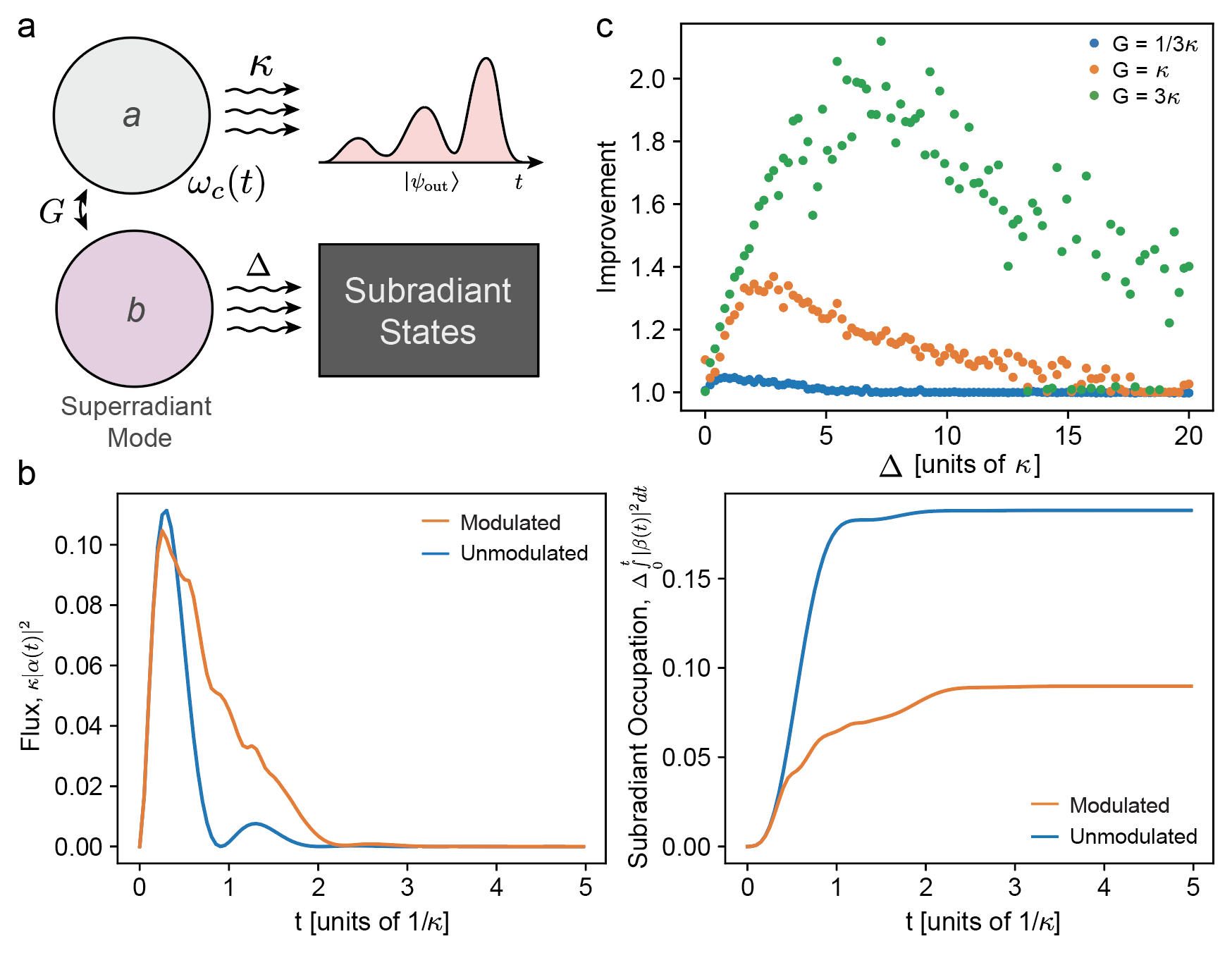
Figure 3: Large $N$ Model (a) Effective model for the system presented in Fig 1a when emitter frequencies are drawn from a Lorentzian distribution and $N\rightarrow\infty$. (b) Output photon flux and subradiant occupation for optimized Large $N$ model with $G=3\kappa$ and $\Delta=5\kappa$. (c) Large $N$ optimization improvement scaling with $\Delta$ for $G=1/3\kappa,1\kappa,$ and $3\kappa$.

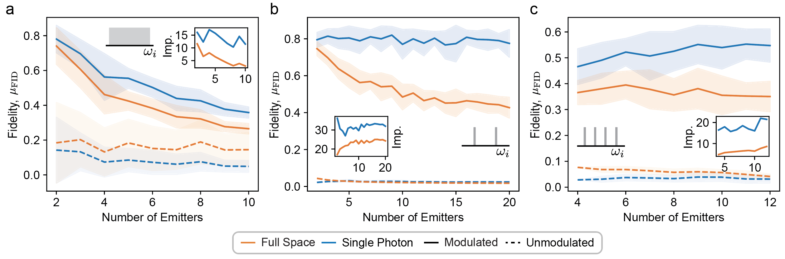
Figure 4: Multi-Photon Optimization (a) Photon emission fidelity normalized to a homogeneous ensemble for the single photon subspace and full space with emitter frequencies drawn from a uniform distribution. Modulation in the both the single photon and full space are optimized in the single photon subspace. Here $g=\kappa/\sqrt{N}$ and $\Delta=10\kappa$. Filled area represents the standard deviation across 25 ensembles. Inset shows average improvement by modulating the system with the optimized pulse. (b) Photon emission fidelity and improvement with emitter frequencies drawn from 2 bins with standard deviation the same as in (a). (c) Photon emission fidelity and improvement with emitter frequencies drawn from 4 bins with standard deviation the same as in (a).

Surprisingly, a constant enhancement in the superradiance metrics persists even in the limit of a large number of emitters, and improves with an increase in the spectral disorder. To confirm and provide an explanation of this behaviour, we derive an effective analytical model for directly capturing the dynamics in the thermodynamic limit ($N\to\infty$). Assuming a Lorentzian distribution of the emitter frequency [$p(\omega_{i})=\Delta_{0}/\pi(\omega_{i}^{2}+\Delta_{0}^{2})$], the single-excitation dynamics in the limit of $N\to\infty$ can be captured by a coupled oscillator model (Fig. 3a) —

$$\begin{bmatrix}\dot{\alpha}(t)\\ \dot{\beta}(t)\end{bmatrix}=\begin{bmatrix}-(i\omega_{c}(t)+\kappa/2)&-G\\ G&-\Delta_{0}\end{bmatrix}\begin{bmatrix}\alpha(t)\\ \beta(t)\end{bmatrix}-iG\begin{bmatrix}e^{-\delta_{0}t}\\ 0\end{bmatrix}.$$ (4)

Here $G=\lim_{N\to\infty}g(N)\sqrt{N}$, and $\alpha(t)$ is the amplitude of the dynamically modulated cavity mode, and $\beta(t)$ can be interpreted as the amplitude of the superradiant mode which directly couples to the cavity mode. Note that the inhomogeneous broadening $\Delta_{0}$ effectively induces a decay in the superradiant mode due to its coupling to the subradiant states due to the inhomogeniety in the emitter frequencies. By optimizing the single photon generation fidelity with this effective model, we find an enhancement in superradiance (Fig 3b) consistent with the finite $N$ results. We clearly see that the application of the modulation reduces the number of photons lost to the subradiant states, and can be viewed as dynamically decoupling the subradiant states from the superradiant mode Viola et al. (1999). Fig. 3c shows the dependence of the improvement in the photon-generation fidelity achieved by the modulation on the coupling strength $G$ and the broadening $\Delta$ — as is intuitively expected, higher improvement in superradiance is seen for more strongly coupled systems. Furthermore, the improvement in single photon generation initially grows with $\Delta$, but tends back towards 1 as $\Delta\gg G$ as the decay into the subradiant bath dominates the system dynamics.

Finally, we study how superradiance within the multi-photon subspaces is impacted by the dynamical modulation. While it is in principle possible to recompute the modulation signal $\omega_{c}(t)$ by simulating an $N$ excitation problem where all the emitters are initially excited (demonstrated in the supplemental information), the cost of performing this simulation increases exponentially with $N$. However, physical intuition suggests that the pulse obtained by maximizing the single-photon superradiance facilitates the transfer of excitations between the disordered ensemble of emitters and the cavity mode, and hence should also enhance superradiance within the full $N-$excitation subspace. We see this effect in the photon emission fidelity in Fig. 4a — we point out that the enhancement obtained for the $N-$excitation problem is smaller than that obtained for the single-particle problem, since the pulse designed within the single-photon space is conceivably suboptimal for the $N-$excitation problem.

An important question that arises for the $N-$excitation superradiance enhancement is whether it survives in the limit of large $N$. Since numerical simulations of the large $N$ model becomes prohibitively expensive, we instead consider the emitter frequencies to be chosen randomly only from a discrete set (Figs. 4b and c) as opposed to a continuous distribution. Exploiting the permutational invariance of emitters at the same frequency, this system can be simulated with a cost that scales polynomially in the number of emitters but exponentially in the number of frequencies Shammah et al. (2018). We expect the discrete probability distribution to at least qualitatively capture the properties of the continuous probability distribution, since it should in principle be possible discretize a continuous probability distribution over the emitter frequencies into bins whose widths depend on the linewidth of the system. While we do not have a rigorous proof of this statement, we numerically verify this for the problem of computing the fidelity metric in the supplement. Figures 4b and c show the dependence of the fidelity on $N$ for $2$ and $4$ frequency problems, we find that the enhancement in superradiance on applying a pulse optimized in the single photon subspace remains nearly constant with $N$ in both cases, indicating that a multiplicative enhancement is possible even in $N-$excitation superradiance.

In conclusion, we have studied a dynamically modulated Tavis-Cummings Hamiltonian with spectral disorder and presented an analysis of the emergence of superradiance in this model. Our conclusions indicate that superradiance can persist and be potentially technologically useful even in the limit of large spectral disorder, and that global quantum controls can be used to enhance it. These results are relevant to a number of on-going experimental efforts in studying and scaling-up solid-state quantum optical systems. One of the most important and interesting problems left open in our work is scaling quantum control designs, with experimentally realistic local or quasi-local controls, to multi-excitation subspaces of systems with large number of emitters. While we explored how controls designed with low excitation number subspaces can provide some improvement even in the high excitation number subspaces, there might be the potential to design controls within the low entanglement spaces of the Hilbert space (i.e. states described by low bond dimension matrix product states), which have been investigated in the context of waveguide QED systems with spatial disorder Manzoni et al. (2017).

Acknowledgments: We thank Sattwik Deb Mishra and Daniel Malz for helpful discussions and Geun Ho Ahn and Eric Rosenthal for providing feedback on the manuscript. AW acknowledges the Herb and Jane Dwight Stanford Graduate Fellowship and the NTT Research Fellowship. RT acknowledges Max Planck Harvard research center for quantum optics (MPHQ) postdoctoral fellowship. KN acknowledges the Stanford Physics Undergraduate Research Program. We acknowledge support from the Department of Energy (DOE) grant number DE-SC0019174.

Supplemental Information

Numerical Techniques

To simulate in the single-photon subspace, we use the time-dependent Schrodinger Equation:

$$i\frac{d}{dt}\ket{\psi_{\text{cav}}(t)} =(\omega_{c}(t)-i\frac{\kappa}{2})\ket{\psi_{\text{cav}}(t)}+g\sum_{i=1}^{N}\ket{\psi_{\text{em},i}(t)}$$

$$i\frac{d}{dt}\ket{\psi_{\text{em},i}(t)} =(\omega_{i}-i\frac{\gamma}{2})\ket{\psi_{\text{em},i}(t)}+g(N)\ket{\psi_{\text{cav}}(t)},$$

where $\omega_{c}(t)$ is the time dependent frequency of the cavity, $\omega_{i}$ is the resonant frequency of the $i$th emitter, and $g(N)$ is the emitter-cavity coupling strength. The cavity emits into an output channel with decay rate $\kappa$, and the emitters in addition to coupling to the cavity also individually decay with decay rate $\gamma$. We initialize the system to $\ket{\psi(0)}=\frac{1}{\sqrt{N}}\sum_{i=1}^{N}\ket{\psi_{\text{em},i}(t)}$.

To simulate in the multi-photon subspace, we use the time-dependent Master Equation:

$$\frac{d}{dt}\rho(t) =-i[H(t),\rho]+\sum_{j=0}^{N}\left[L_{j}\rho L_{j}^{\dagger}-\frac{1}{2}\{L_{j}^{\dagger}L_{j},\rho\}\right],\ \text{where}$$

$$H(t) =\omega_{c}(t)a^{\dagger}a+\sum_{i=1}^{N}\omega_{i}\sigma_{i}^{\dagger}\sigma_{i}+g(N)\sum_{i=1}^{N}(a^{\dagger}\sigma_{i}+\sigma_{i}^{\dagger}a),$$

$$L_{0} =\sqrt{\kappa}a,$$

$$L_{j} =\sqrt{\gamma}\sigma_{j}\ \text{for }j=1,2\dots N,$$

where $\omega_{c}(t)$ is the time dependent frequency of the cavity, $\omega_{i}$ is the resonant frequency of the $i$th emitter, $a^{\dagger}$ is the raising operator of the cavity, $\sigma_{i}^{\dagger}$ is the excitation operator of the $i$th emitter, and $g(N)$ is the emitter-cavity coupling strength. Furthermore, we assume that the cavity emits into an output channel with decay rate $\kappa$, and the emitters in addition to coupling to the cavity also individually decay with decay rate $\gamma$. We initialize the system to the excited state of all emitters.

Adjoint Optimization

We consider a general problem of a state $s(t)$ governed by

$$\frac{ds(t)}{dt}=A(t,p)s(t)+b(t),$$ (5)

where $p$ are control parameters governing the trajectory of the system and $b(t)$ is the input to the system. The system at $t=0$ is at state $s(0)$ and the time window of interest is from $t=0$ to $t=T$. We consider an objective function $O$:

$$O=f\left(\int_{0}^{T}\sigma^{\text{T}}(t)s(t)dt\right),$$ (6)

where $f:\mathbb{C}\rightarrow\mathbb{R}$ is some function. We are interested in computing $\partial O/\partial p_{i}$ efficiently.

Preliminaries: Formally, the solution of the ODE can be written by introducing the propagator $U(t)$:

$$U(t,p)=\mathrm{T}e^{\int_{0}^{t}A(\tau,p)d\tau}$$ (7)

to reach

$$s(t)=U(t,p)s(0)+U(t,p)\int_{0}^{t}U^{-1}(\tau,p)b(\tau)d\tau.$$ (8)

An ODE for $U^{-1}(t,p)$ can also be calculated,

$$\frac{d}{dt}U^{-1}(t,p)+U^{-1}(t,p)A(t,p)=0.$$ (9)

Calculation of gradient: Consider perturbing $p_{i}\rightarrow p_{i}+\delta p_{i}$. This would result in the state $s(t)\rightarrow s(t)+\delta s(t)$, where

$$\frac{d}{dt}\delta s(t)=U(t,p)\int_{0}^{t}U^{-1}(\tau,p)\frac{\partial A(\tau,p)}{\partial p_{i}}s(\tau)d\tau,$$ (10)

the solution to which is given by

$$\frac{\delta s(t)}{\delta p_{i}}=U(t,p)\int_{0}^{t}U^{-1}(\tau,p)\frac{\partial A(\tau,p}{\partial p_{i}}s(\tau)d\tau,$$ (11)

where we have used the fact that $\delta s(0)=0$. Now the objective function changes by

$$\frac{\delta O}{\delta p_{i}}=2\mathrm{Re}\left\{f^{\prime}\left(\int_{0}^{T}\sigma^{\text{T}}(t)s(t)dt\right)\int_{0}^{T}\sigma^{\text{T}}(t)\frac{\delta s(t)}{\delta p_{i}}dt\right\}.$$ (12)

Consider the term

$$\int_{0}^{T}\sigma^{\text{T}}(t)\frac{\delta s(t)}{\delta p_{i}}dt$$

$$=\int_{t=0}^{T}\int_{\tau=0}^{t}\sigma^{\text{T}}(t)U(t,p)U^{-1}(\tau,p)\frac{\partial A(\tau,p)}{\partial p_{i}}s(\tau)d\tau dt$$

$$=\int_{\tau=0}^{T}\int_{t=\tau}^{T}\sigma^{\text{T}}(t)U(t,p)U^{-1}(\tau,p)\frac{\partial A(\tau,p)}{\partial p_{i}}s(\tau)d\tau dt$$

$$=\int_{\tau=0}^{T}a^{\text{T}}(t)\frac{\partial A(\tau,p)}{\partial p_{i}}s(\tau)d\tau,$$

where we have defined

$$a(\tau)=\int_{t=\tau}^{T}[U(t,p)U^{-1}(t,p)]^{\text{T}}\sigma(t)dt$$

$$=U^{-\text{T}}(\tau,p)\int_{t=\tau}^{T}U^{\text{T}}(t,p)\sigma(t)dt.$$

An ODE for $a(t)$ can now be derived:

$$\frac{d}{d\tau}a(\tau) =\frac{d}{d\tau}U^{-\text{T}}(\tau,p)\int_{t=\tau}^{T}U^{T}(t,p)\sigma(t)dt$$

$$\qquad\qquad+U^{-\text{T}}(\tau,p)(-U^{\text{T}}(\tau,p)\sigma(\tau))$$

$$=[-U^{-1}(\tau,p)A(\tau,p)]^{\text{T}}\int_{t=\tau}^{T}U^{\text{T}}(t,p)\sigma(t)dt-\sigma(\tau)$$

$$=-A^{\text{T}}(\tau,p)a(\tau)-\sigma(\tau).$$

The boundary condition, as seen from the definition is simply $a(T)=0$. This is the adjoint simulation. Finally, for the gradient we obtain

$$\frac{\delta O}{\delta p_{i}}=2\mathrm{Re}\left\{f^{\prime}\left(\int_{0}^{T}\sigma^{\text{T}}(t)s(t)dt\right)\int_{0}^{T}a^{\text{T}}(\tau)\frac{\partial A(\tau,p)}{\partial p_{i}}s(\tau)d\tau\right\}.$$ (13)

We note that the adjoint field is calculated only once, and all the derivatives $\delta O/\delta p_{i}$ are accessed immediately.

In our specific problem, the state evolution $s(t)=\psi(t)$ is governed by the system Hamiltonian, so

$$A(t,p)=H(t)=\omega_{c}(t)a^{\dagger}a+\sum_{i=1}^{N}\omega_{i}\sigma_{i}^{\dagger}\sigma_{i}+g\sum_{i=1}^{N}(a^{\dagger}\sigma_{i}+\sigma_{i}^{\dagger}a),$$

and the free parameter $p$ corresponds to $\omega_{c}(t)$. Thus the gradient with respect to our one free parameter is

$$\frac{\partial A(t,p)}{\partial p}=a^{\dagger}a$$

We can calculate the output wave function by taking the overlap of the system wave function with the cavity state, and so our overlap objective is

$$\sigma^{\text{T}}(t)=f(t)\bra{\text{G}}a,$$

where $f(t)$ is the desired time dependent wavefunction (which we compute from the simulation of the homogeneous system).

As our objective function is the absolute value squared of the overlap, our gradients can be calculated as

$$\frac{\delta O}{\delta\omega_{c}(t)}=2\text{Re}\left\{\bra{a(t)}a^{\dagger}a\ket{\psi(t)}\int_{0}^{T}f^{*}(\tau)\braket{G}{a}{\psi(\tau)}^{*}d\tau\right\}.$$

Large $N$ Model

To derive a model for the limit of a large number of emitters, we first need to derive the system dynamics as a function of the emitter distribution.

We start with the single particle problem

$$\ket{\psi(t)}=\left[\alpha(t)a^{\dagger}+\sum_{\mu=1}^{N}s_{\mu}(t)\sigma_{\mu}^{\dagger}\right]\ket{0}$$ (14)

which is governed by

$$i\dot{\alpha}(t) =\left(\omega_{c}(t)-i\frac{\kappa}{2}\right)\alpha(t)+\frac{G}{\sqrt{N}}\sum_{\mu=1}^{N}s_{\mu}(t)$$

$$i\dot{s}_{\mu}(t) =\delta_{\mu}s_{\mu}(t)+\frac{G}{\sqrt{N}}\alpha(t).$$

We can integrate the second equation of motion

$$s_{\mu}(t)=s_{\mu}(0)e^{-i\delta_{\mu}t}-i\frac{G}{\sqrt{N}}\int_{0}^{t}\alpha(s)e^{-i\delta_{\mu}(t-s)}ds.$$

Thus,

$$\sum_{\mu=1}^{N}s_{\mu}(t)=\sqrt{N}S_{in}(t)-i\sum_{\mu=1}^{N}\frac{G}{\sqrt{N}}\int_{0}^{t}\alpha(s)e^{-i\delta_{\mu}(t-s)}ds,$$

where we have introduced

$$S_{\text{in}}(t)=\sum_{\mu=1}^{N}S_{\mu}(0)\frac{e^{-i\delta_{\mu}t}}{\sqrt{N}}.$$ (15)

Thus,

$$i\dot{\alpha}(t)=\left(\omega_{c}(t)-i\frac{\kappa}{2}\right)\alpha -i\frac{G^{2}}{N}\sum_{\mu=1}^{N}\int_{0}^{t}\alpha(s)e^{-i\delta_{\mu}(t-s)}ds-iGS_{\text{in}}(t)$$

$$i\dot{\alpha}(t)=\left(\omega_{c}(t)-i\frac{\kappa}{2}\right)\alpha -iG^{2}\int_{0}^{t}\alpha(s)K(t-s)ds-iGS_{\text{in}}(t),$$

where for $t\geq 0$

$$K(t)=\frac{1}{N}\sum_{\mu=1}^{N}e^{-i\delta_{\mu}t}.$$

We now have an expression for the cavity dynamics as a function of the emitter frequencies. Until this point, the system of equations is exact. Assuming each frequency is picked independently at random, in the limit of large $N$, $K(t)$ can be expressed as

$$K(t)=\braket{e^{-i\delta t}}=\int P(\delta)e^{-i\delta t}d\delta.$$ (16)

A relatively simple model can be derived if $P(\delta$) is Lorentzian,

$$P(\delta)=\frac{\delta_{0}}{\pi}\frac{1}{\delta^{2}+\Delta_{0}^{2}}.$$

In this case, for $t\geq 0$

$$K(t) =\frac{\delta_{0}}{\pi}\int_{-\infty}^{\infty}\frac{e^{-i\delta t}}{\delta^{2}+\Delta_{0}^{2}}d\delta$$

$$=\frac{1}{2\pi i}\int_{-\infty}^{\infty}\left(\frac{1}{\delta-i\Delta_{0}}-\frac{1}{\delta+i\Delta_{0}}\right)e^{-i\delta t}d\delta$$

$$=e^{-\Delta_{0}t}.$$

Now, introducing $\beta(t)$ as

$$\beta(t) =G\int_{0}^{t}\alpha(s)K(t-s)ds$$

$$=G\int_{0}^{t}e^{-\Delta_{0}(t-s)}\alpha(s)ds,$$

we can rewrite the equations of motion as

$$\dot{\alpha}(t) =-i\left(\omega_{c}(t)-i\frac{\kappa}{2}\right)\alpha-G\beta(t)-iGS_{\text{in}}(t)$$

$$\dot{\beta}(t) =-\Delta_{0}\beta(t)+G\alpha(t)$$

which is a model of a coupled cavity (Fig 3a). Here, $\alpha(t)$ still represents the original cavity, and the new $\beta(t)$ represents the superradiant state. The decay rate $\Delta_{0}$ of the superradiant state $\beta(t)$ can be viewed as the decay into a bath consisting of the subradiant states, whose coupling rate to the cavity are 0 in the limit of large $N$.

To simulate an initial state which is an equal superposition of all excited states, we would use $S_{\mu}(0)=1/\sqrt{N}$ with which

$$S_{\text{in}}(t) =\frac{1}{N}\sum_{\mu}e^{-i\delta_{\mu}t}$$

$$=\braket{e^{-i\delta t}}$$

$$=\int P(\delta)e^{-i\delta t}d\delta$$

$$=e^{-\Delta_{0}t}u(t),$$

where $u(t)$ is the unit step function. As $S_{in}(t)$ is the only input to the system, it bounds the maximum single photon generation fidelity. As the total power entering into the system, $\int_{0}^{\infty}GS_{in}(t)dt$, scales as $G/\Delta_{0}$, the maximum possible fidelity should scale accordingly.

Multi-photon Optimization

By maximizing the overlap of the full $N$-photon output wavepacket with that of the homogeneous case, we can enhance the emission rate of 2 to 5 emitter inhomogeneous ensembles, Sup. Fig. 1. However, this optimization procedure is far too expensive for larger $N$, as the simulation costs scales exponentially.

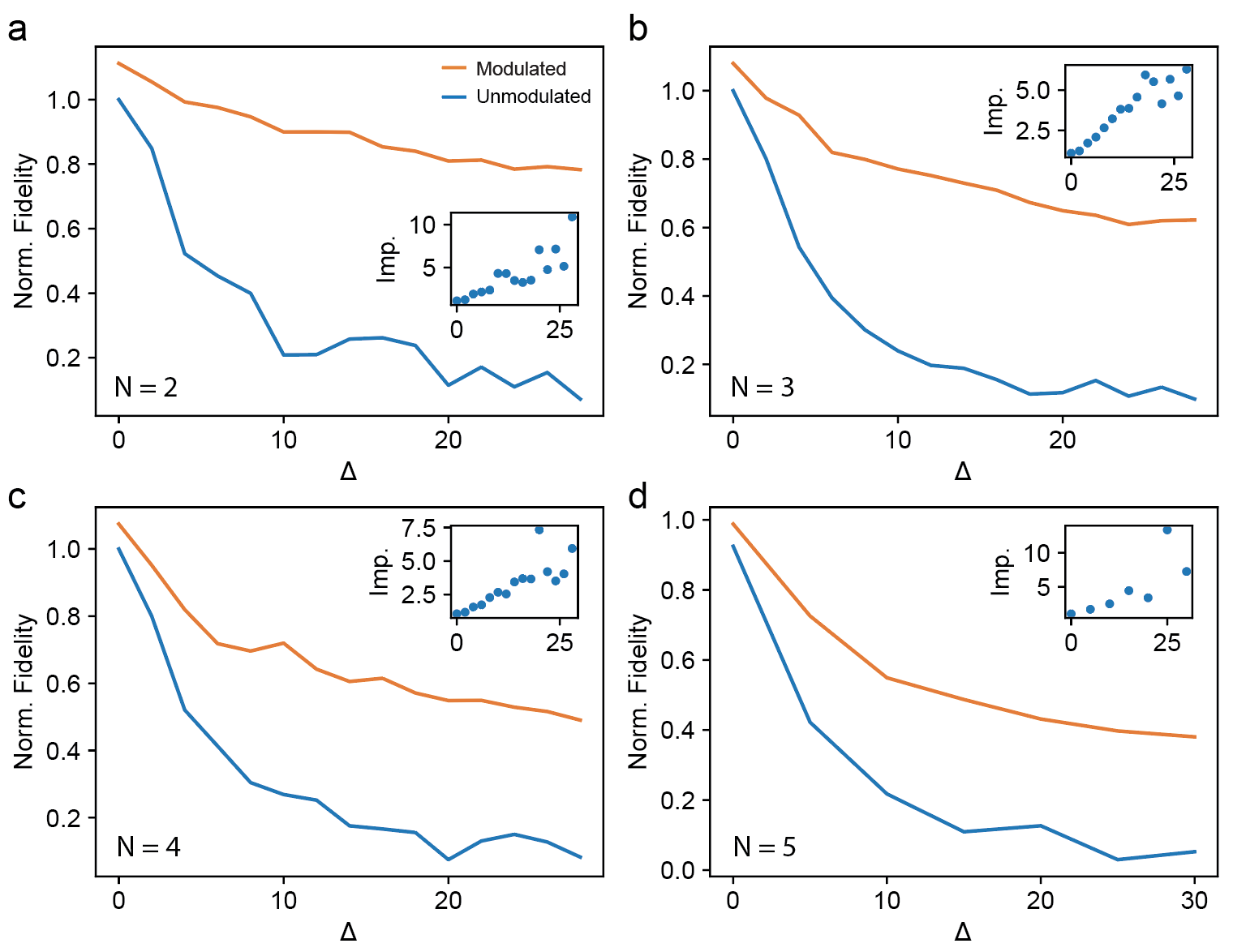
Figure S1: $N$ Photon Multi-Emitter Optimization (a-d) $N$ photon space optimization of $N=2,3,4,5$ emitters with a nonradiative decay rate of $0.5\kappa$ and $\Delta$ in units of $\kappa$. All data points are an average of 25 ensembles.

To simulate larger ensembles more efficiently, we can bin the emitter frequencies in order to maximize permutational invariance, allowing the simulation to scale polynomially with the number of emitters and exponentially only with the number of frequency bins. To validate that this discretization can still capture the desired system dynamics, we calculate the simulation error in single photon generation fidelity with increasing $N$, Sup. Fig. 2a. Here we define the simulation error as the fractional difference in fidelity between the discretized ensemble and full ensemble. We find that the error induced through discretization can be made to be small with enough bins, and also that the number of bins needed for a given error threshold does not increase with the number of emitters (given that g scales as $1/\sqrt{N}$). For a given $N$, we also find that the error introduced by binning decreases as $g$ is increased, Sup. Fig. 2b,likely because the linewidths of the emitters grow, increasing the minimum linewidth of the system.

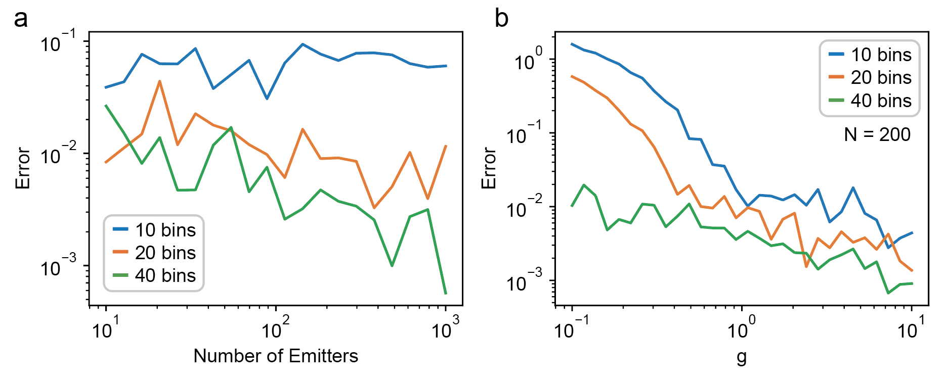
Figure S2: Emitter Binning (a) Error in calculated single photon generation fidelity due to binning as N increases. Here $\Delta=10\kappa$, $g=\kappa/\sqrt{N}$. (b) Error in calculated single photon generation fidelity due to binning as $g$ increases for $N=200$. $g$ is in units of $\kappa/\sqrt{200}$.

References

- Tavis and Cummings (1968) M. Tavis and F. W. Cummings, Physical Review 170, 379 (1968).
- Gross and Haroche (1982) M. Gross and S. Haroche, Physics reports 93, 301 (1982).
- Rehler and Eberly (1971) N. E. Rehler and J. H. Eberly, Physical Review A 3, 1735 (1971).
- Scully and Svidzinsky (2009) M. O. Scully and A. A. Svidzinsky, Science 325, 1510 (2009).
- Dicke (1954) R. H. Dicke, Physical review 93, 99 (1954).
- Andreev et al. (1980) A. V. Andreev, V. I. Emel’yanov, and Y. A. Il’inskiĭ, Soviet Physics Uspekhi 23, 493 (1980).
- Clemens et al. (2003) J. Clemens, L. Horvath, B. Sanders, and H. Carmichael, Physical Review A 68, 023809 (2003).
- Eleuch and Rotter (2014) H. Eleuch and I. Rotter, The European Physical Journal D 68, 1 (2014).
- Hepp and Lieb (1973) K. Hepp and E. H. Lieb, Annals of Physics 76, 360 (1973).
- Lambert et al. (2004) N. Lambert, C. Emary, and T. Brandes, Physical review letters 92, 073602 (2004).
- Bamba et al. (2016) M. Bamba, K. Inomata, and Y. Nakamura, Physical review letters 117, 173601 (2016).
- Casabone et al. (2015) B. Casabone, K. Friebe, B. Brandstätter, K. Schüppert, R. Blatt, and T. Northup, Physical review letters 114, 023602 (2015).
- Ortiz-Gutiérrez et al. (2018) L. Ortiz-Gutiérrez, L. Muñoz-Martínez, D. Barros, J. Morales, R. Moreira, N. Alves, A. Tieco, P. Saldanha, and D. Felinto, Physical review letters 120, 083603 (2018).
- Jahnke et al. (2016) F. Jahnke, C. Gies, M. Aßmann, M. Bayer, H. Leymann, A. Foerster, J. Wiersig, C. Schneider, M. Kamp, and S. Höfling, Nature communications 7, 1 (2016).
- Scheibner et al. (2007) M. Scheibner, T. Schmidt, L. Worschech, A. Forchel, G. Bacher, T. Passow, and D. Hommel, Nature Physics 3, 106 (2007).
- Grim et al. (2019) J. Q. Grim, A. S. Bracker, M. Zalalutdinov, S. G. Carter, A. C. Kozen, M. Kim, C. S. Kim, J. T. Mlack, M. Yakes, B. Lee, et al., Nature materials 18, 963 (2019).
- Angerer et al. (2018) A. Angerer, K. Streltsov, T. Astner, S. Putz, H. Sumiya, S. Onoda, J. Isoya, W. J. Munro, K. Nemoto, J. Schmiedmayer, et al., Nature Physics 14, 1168 (2018).
- Zhong et al. (2017) T. Zhong, J. M. Kindem, J. Rochman, and A. Faraon, Nature communications 8, 1 (2017).
- Anderson (1958) P. W. Anderson, Physical review 109, 1492 (1958).
- Lee and Fisher (1981) P. A. Lee and D. S. Fisher, Physical Review Letters 47, 882 (1981).
- Alet and Laflorencie (2018) F. Alet and N. Laflorencie, Comptes Rendus Physique 19, 498 (2018).
- Nandkishore and Huse (2015) R. Nandkishore and D. A. Huse, Annu. Rev. Condens. Matter Phys. 6, 15 (2015).
- Pal and Huse (2010) A. Pal and D. A. Huse, Physical review b 82, 174411 (2010).
- Nandkishore and Sondhi (2017) R. M. Nandkishore and S. L. Sondhi, Physical Review X 7, 041021 (2017).
- Nag and Garg (2019) S. Nag and A. Garg, Physical Review B 99, 224203 (2019).
- Smith et al. (2016) J. Smith, A. Lee, P. Richerme, B. Neyenhuis, P. W. Hess, P. Hauke, M. Heyl, D. A. Huse, and C. Monroe, Nature Physics 12, 907 (2016).
- Moreira et al. (2019) N. A. Moreira, R. Kaiser, and R. Bachelard, EPL (Europhysics Letters) 127, 54003 (2019).
- Akkermans et al. (2008) E. Akkermans, A. Gero, and R. Kaiser, Physical review letters 101, 103602 (2008).
- Ashhab and Semba (2017) S. Ashhab and K. Semba, Physical Review A 95, 053833 (2017).
- Biella et al. (2013) A. Biella, F. Borgonovi, R. Kaiser, and G. Celardo, EPL (Europhysics Letters) 103, 57009 (2013).
- Cottier et al. (2018) F. Cottier, R. Kaiser, and R. Bachelard, Physical Review A 98, 013622 (2018).
- Kelly et al. (2021) S. P. Kelly, A. M. Rey, and J. Marino, Physical Review Letters 126, 133603 (2021).
- Manzoni et al. (2017) M. T. Manzoni, D. E. Chang, and J. S. Douglas, Nature communications 8, 1 (2017).
- Fayard et al. (2021) N. Fayard, L. Henriet, A. Asenjo-Garcia, and D. Chang, arXiv preprint arXiv:2101.01645 (2021).
- Temnov and Woggon (2005) V. V. Temnov and U. Woggon, Physical review letters 95, 243602 (2005).
- Trivedi et al. (2019) R. Trivedi, M. Radulaski, K. A. Fischer, S. Fan, and J. Vučković, Physical review letters 122, 243602 (2019).
- Mivehvar et al. (2017) F. Mivehvar, F. Piazza, and H. Ritsch, Physical review letters 119, 063602 (2017).
- Debnath et al. (2019) K. Debnath, Y. Zhang, and K. Mølmer, Physical Review A 100, 053821 (2019).
- Zhang et al. (2019) M. Zhang, C. Wang, Y. Hu, A. Shams-Ansari, T. Ren, S. Fan, and M. Lončar, Nature Photonics 13, 36 (2019).
- Sun et al. (2018) S. Sun, J. L. Zhang, K. A. Fischer, M. J. Burek, C. Dory, K. G. Lagoudakis, Y.-K. Tzeng, M. Radulaski, Y. Kelaita, A. Safavi-Naeini, et al., Physical review letters 121, 083601 (2018).
- Lukin et al. (2020) D. M. Lukin, A. D. White, et al., npj Quantum Information 6, 1 (2020).
- De Fouquieres et al. (2011) P. De Fouquieres, S. Schirmer, S. Glaser, and I. Kuprov, Journal of Magnetic Resonance 212, 412 (2011).
- d’Alessandro (2007) D. d’Alessandro, Introduction to quantum control and dynamics (Chapman and Hall/CRC, 2007).
- Julsgaard et al. (2013) B. Julsgaard, C. Grezes, P. Bertet, and K. Mølmer, Physical review letters 110, 250503 (2013).
- Gorshkov et al. (2008) A. V. Gorshkov, T. Calarco, M. D. Lukin, and A. S. Sørensen, Physical Review A 77, 043806 (2008).
- Aizenman and Molchanov (1993) M. Aizenman and S. Molchanov, Communications in Mathematical Physics 157, 245 (1993).
- Trivedi et al. (2018) R. Trivedi, K. Fischer, S. Xu, S. Fan, and J. Vuckovic, Physical Review B 98, 144112 (2018).
- Fischer et al. (2018) K. A. Fischer, R. Trivedi, V. Ramasesh, I. Siddiqi, and J. Vučković, Quantum 2, 69 (2018).
- Cao et al. (2003) Y. Cao, S. Li, L. Petzold, and R. Serban, SIAM journal on scientific computing 24, 1076 (2003).
- Viola et al. (1999) L. Viola, E. Knill, and S. Lloyd, Physical Review Letters 82, 2417 (1999).
- Shammah et al. (2018) N. Shammah, S. Ahmed, N. Lambert, S. De Liberato, and F. Nori, Physical Review A 98, 063815 (2018).