An EMA-conserving, pressure-robust and Re-semi-robust reconstruction method for the unsteady incompressible Navier-Stokes equations

Abstract.

Proper EMA-balance (E: kinetic energy; M: momentum; A: angular momentum), pressure-robustness and $Re$-semi-robustness ($Re$: Reynolds number) are three important properties of Navier-Stokes simulations with exactly divergence-free elements. This EMA-balance makes a method conserve kinetic energy, linear momentum and angular momentum under some suitable senses; pressure-robustness means that the velocity errors are independent of the continuous pressure; $Re$-semi-robustness means that the constants appearing in the error bounds of kinetic and dissipation energies do not explicitly depend on inverse powers of the viscosity. In this paper, based on the pressure-robust reconstruction methods in [A. Linke and C. Merdon, Comput. Methods Appl. Mech. Engrg. 311 (2016), 304-326], we propose a novel reconstruction method for a class of non-divergence-free simplicial elements which admits almost all the above properties. The only exception is the energy balance, where kinetic energy should be replaced by a properly redefined discrete energy. Some numerical comparisons with exactly divergence-free methods, pressure-robust reconstructions and the EMAC scheme are provided to confirm our theoretical results.

1. Introduction

In this paper, we study the finite element methods for the unsteady Navier-Stokes equations (NSEs):

(1.1a) $$\boldsymbol{u}_{t}-\nu\Delta\boldsymbol{u}+\left(\boldsymbol{u}\cdot\nabla\right)\boldsymbol{u}+\nabla p =\boldsymbol{f} \text{in}~{}J\times\Omega,$$

(1.1b) $$\nabla\cdot\boldsymbol{u} =0 \text{in}~{}J\times\Omega,$$

(1.1c) $$\boldsymbol{u}\left(0\right) =\boldsymbol{u}^{0} \text{in}~{}\Omega,$$

(1.1d) $$\boldsymbol{u} =\boldsymbol{0} \text{on}~{}J\times\Gamma,$$

where $J=\left(0,T\right]$ and $\Omega\subset\mathbb{R}^{d}$ $\left(d=2,3\right)$ is a bounded domain with Lipschitz-continuous polyhedral boundary $\Gamma$; $\boldsymbol{u}$ and $p$ represent the unknown velocity and pressure, respectively; $\nu>0$ is the constant kinematic viscosity; $\boldsymbol{f}$ represents the external force and $\boldsymbol{u}^{0}$ is the initial velocity. We assume $\boldsymbol{f}\left(t\right)\in\boldsymbol{L}^{2}\left(\Omega\right)$ for all $t\in J$. For simplicity, here we only consider the homogeneous Dirichlet boundary condition. Other boundary conditions are also of interest.

For designing accurate numerical schemes, it is widely believed that preserving the fundamental (physical or mathematical) properties of the continuous problem is of great importance. For the unsteady incompressible Navier-Stokes equations, these fundamental properties include the divergence constraint eq. 1.1b, the balance laws for some physical quantities (e.g., kinetic energy, linear momentum, angular momentum, vorticity, helicity and enstrophy) [18, 10], an invariance property for the velocity with respect to the gradient field in $\boldsymbol{f}$ [35, 30] and so on. Among these properties, the divergence constraint is of central importance. The papers [18, 30] respectively showed that the exactly divergence-free mixed methods preserved the balance laws and the invariance property mentioned above. The latter means that these methods are pressure-robust; namely the velocity errors are independent of the pressure. Moreover, it was demonstrated in [46] that the constants in error estimates, including the Gronwall constant, did not depend on $\nu^{-1}$ explicitly for divergence-free finite element methods. This property was called ($Re$-)semi-robustness, uniform, or quasi-uniform estimates [29] sometimes.

Due to these fascinating properties, constructing exactly divergence-free elements has been an increasingly hot topic in recent years [49, 25, 26, 39, 27, 12, 40]. However, compared to classical non-divergence-free elements (e.g., Taylor-Hood, MINI and Bernardi-Raugel, cf. [23, 28]), the construction of these elements is not trivial in most cases. Another popular idea is relaxing the continuity condition but enforcing the divergence constraint strongly, which results in the so-called nonconforming $H(\operatorname{div})$-conforming methods [14, 48, 47, 31, 24, 45]. In this paper, we focus on the conforming mixed methods for the Navier-Stokes equations.

Modifying the formulation to preserve some fundamental properties of the continuous problem (or divergence-free mixed methods) for non-divergence-free elements is another popular research topic. With an observation that most classical elements are non-divergence-free, this topic includes (not just) pressure-robust reconstructions [35, 36, 37, 32, 34], the EMAC (EMA-conserving) formulation [10, 11, 42] and some $Re$-semi-robust methods [15, 8, 16, 20]. The method introduced in this paper is also included in this topic. Pressure-robustness plays an important role on the accuracy of a method when ‘gradient forces dominate the momentum balance’ [38]; the velocity errors of the methods which are not $Re$-semi-robust might grow quickly with respect to time for higher Reynolds number flows [46]; the EMAC scheme is one of the “enhanced-physics” based schemes which have a long history such as [2, 19, 1, 44, 43], and the paper [42] showed that an improper treatment of energy, linear momentum and angular momentum produced lower bounds for $L^{2}$ velocity errors. It is worth mentioning that, the properties mentioned above are usually not mutually independent. For example, in the paper [42], Olshanskii and Rebholz proved that the Gronwall constants in EMAC estimates did not depend on the viscosity explicitly, which is exactly $Re$-semi-robustness except that the constant in the pressure-induced error polynomially depended on the inverse of viscosity. Another example is the popular grad-div stabilization [41, 9]. It can not only weaken (not totally remove) the impact of the pressure on velocity errors [30] but also make the usual skew-symmetric scheme semi-robust with respect to the Reynolds number [15]. Finally, we also refer the readers to the review article [29] for more details.

In this paper, we propose a novel reconstruction formulation which is EMA-conserving for the reconstructed discrete velocity (here the energy should be redefined), pressure-robust and $Re$-semi-robust. For simplicity, we shall refer to this reconstruction as the “EMAPR” reconstruction throughout this paper. Our method is based on the pressure-robust reconstruction formulation in [37]. The main difference lies on the discretization of the convective term. For the convective term, two (pressure-robust) discrete forms were proposed in [37]: the convective form and the rotational form. Similarly to [10], it can be checked that the two forms do not conserve the linear momentum and angular momentum (the latter conserves kinetic energy). Here we propose an EMA-conserving form, i.e., it does not produce any extra energy, momentum and angular momentum under some appropriate senses. Then we give a pressure-robust and $Re$-semi-robust error estimate for the continuous-in-time case, provided that the continuous solution $\boldsymbol{u}$ is in $L^{2}\left(J;\boldsymbol{W}^{1,\infty}\left(\Omega\right)\right)$. To obtain such an estimate, we also need to slightly modify the discretization of the evolutionary term by introducing a stabilization. Finally, we shall prove that our formulation could be easily applied to a class of simplicial locally mass-conserving elements whose pressures are discontinuous. To the best of our knowledge, the EMAPR reconstruction is the first method on conforming non-divergence-free elements which is EMA-conserving, pressure-robust and $Re$-semi-robust simultaneously. For nonconforming and non-divergence-free methods, a reconstructed Hybrid discontinuous Galerkin method in [33] (see formulas “(6.3d)” and “(6.5)” in it) probably admits most of these properties also.

The remainder of this paper is organized as follows. In Section 2 we discuss the EMAPR methods and some balance laws. Section 3 is devoted to giving a pressure-robust and $Re$-semi-robust error estimate for the EMAPR method. We show that a class of locally divergence-free elements (include the Bernardi-Raugel element) could be easily incorporated into our framework in Section 4. Finally we carry out some numerical experiments in Section 5.

In what follows we will use $C$, with or without a subscript, to denote a generic positive constant. The standard inner product for $\left[L^{2}\left(D\right)\right]^{n}$ or $\left[L^{2}\left(D\right)\right]^{n\times n}$ ($n\in\mathbb{Z}$) will be denoted by $\left(\cdot,\cdot\right)_{D}$ uniformly. The notation $\left\|\cdot\right\|_{m,p,D}$ ($\left|\cdot\right|_{m,p,D}$) will be used to denote the Sobolev norm (seminorm, respectively) of $\left[W^{m,p}\left(D\right)\right]^{n}$ or $\left[W^{m,p}\left(D\right)\right]^{n\times n}$. With the convention the subscripts $m,p$ and $D$ will be omitted for $m=0$, $p=2$ and $D=\Omega$, respectively. $H^{m}\left(D\right)$ coincides with $W^{m,2}\left(D\right)$ and $\boldsymbol{W}^{m,p}\left(D\right)$ coincides with $\left[{W}^{m,p}\left(D\right)\right]^{d}$.

2. The EMAPR reconstruction method

2.1. The divergence-free reconstruction operator

Let $\mathcal{T}_{h}$ denote a partition of $\Omega$. We define the mesh size $h:=\max_{K\in\mathcal{T}_{h}}h_{K}$ with $h_{K}$ the diameter of elements $K$. Denote by $\varrho_{K}$ the diameter of the biggest ball inscribed in $K$. Here we assume that $\mathcal{T}_{h}$ is shape-regular [13], i.e., there exists a positive constant $\xi$ such that

(2.1) $$\frac{h_{K}}{\varrho_{K}}\leq\xi\quad\forall~{}K\in\mathcal{T}_{h}.$$

Introduce

$$V=\boldsymbol{H}^{1}_{0}\left(\Omega\right):=\left\{\boldsymbol{v}\in\boldsymbol{H}^{1}\left(\Omega\right):\boldsymbol{v}|_{\Gamma}=\boldsymbol{0}\right\},$$

$$X=\boldsymbol{H}_{0}\left(\operatorname{div};\Omega\right):=\left\{\boldsymbol{v}\in\boldsymbol{H}\left(\operatorname{div};\Omega\right):\boldsymbol{v}\cdot\boldsymbol{n}\right|_{\Gamma}=0\},$$

$$\boldsymbol{H}^{2}\left(\mathcal{T}_{h}\right):=\left\{\boldsymbol{v}\in\boldsymbol{L}^{2}\left(\Omega\right):\boldsymbol{v}|_{K}\in\boldsymbol{H}^{2}\left(K\right)\quad\forall~{}K\in\mathcal{T}_{h}\right\},$$

and

$$W=L_{0}^{2}\left(\Omega\right):=\left\{q\in L^{2}\left(\Omega\right):\int_{\Omega}q~{}d\boldsymbol{x}=0\right\},$$

where $\boldsymbol{n}$ is the unit external normal vector on $\Gamma$. Furthermore we define the bilinear form $b:X\times W\rightarrow\mathbb{R}$ by

$$b\left(\boldsymbol{v},q\right):=\left(\nabla\cdot\boldsymbol{v},q\right)\ \text{ for any }\ \left(\boldsymbol{v},q\right)\in X\times W.$$

Let $\left(V_{h},X_{h},W_{h}\right)\subset\left(V,X,W\right)$ denotes a triple of finite element spaces satisfying

(2.2) $$\inf_{q_{h}\in W_{h}}\sup_{\boldsymbol{v}_{h}\in V_{h}\setminus\left\{\boldsymbol{0}\right\}}\frac{b\left(\boldsymbol{v}_{h},q_{h}\right)}{\left\|\nabla\boldsymbol{v}\right\|}\geq\beta_{h}\left\|q_{h}\right\|\text{ for some }\beta_{h}>0,$$

and

(2.3) $$\nabla\cdot X_{h}\subseteq W_{h}.$$

Remark 1.

For simplicity, throughout this article we assume that $\boldsymbol{u}\notin V_{h}$ for the true solution $\boldsymbol{u}$. This assumption does not influence the construction of the method, but will be beneficial to simplifying notation in error estimates and highlighting the fundamental ideas. For a more general velocity, there is no extra essential difficulty for analysis.

Denote by

$$V^{0}:=\left\{\boldsymbol{v}\in V:b\left(\boldsymbol{v},q\right)=0\quad\forall~{}q\in W\right\}=\left\{\boldsymbol{v}\in V:\nabla\cdot\boldsymbol{v}=0\right\},$$

and

$$V_{h}^{0}:=\left\{\boldsymbol{v}_{h}\in V_{h}:b\left(\boldsymbol{v}_{h},q_{h}\right)=0\quad\forall~{}q_{h}\in W_{h}\right\},$$

the spaces of divergence-free velocity functions and discretely divergence-free velocity functions, respectively. Note that if $\nabla\cdot V_{h}\subseteq W_{h}$, we have $V_{h}^{0}\subset V^{0}$, which means that the functions in $V_{h}^{0}$ are exactly divergence-free. For most classical elements, this relationship does not hold.

Let $P^{k}\left(K\right)$ denotes the space of polynomials on $K$ of degree no more than $k$. We also define

$$\boldsymbol{P}^{k}:=\left\{\boldsymbol{v}_{h}\in V:\boldsymbol{v}_{h}|_{K}\in\left[P^{k}(K)\right]^{d}\text{ for all }K\in\mathcal{T}_{h}\right\}.$$

We suppose that the velocity space $V_{h}$ is of order $k$ ($k\geq 1$), i.e., there exists a non-negative integer $k$ such that $\boldsymbol{P}^{k}\subset V_{h}$ and $\boldsymbol{P}^{k+1}\not\subset V_{h}$.

We introduce the divergence-free reconstruction operator $\Pi_{h}:V_{h}\rightarrow X_{h}$ (we do not give the concrete definition here) which satisfies that

(2.4) $$\nabla\cdot\Pi_{h}\boldsymbol{v}_{h}\equiv 0\text{ for all }\boldsymbol{v}_{h}\in V_{h}^{0};$$

(2.5) $$b\left(\boldsymbol{v}_{h},q_{h}\right)=b\left(\Pi_{h}\boldsymbol{v}_{h},q_{h}\right)\text{ for all }\left(\boldsymbol{v}_{h},q_{h}\right)\in V_{h}\times W_{h};$$

(2.6) $$\left(\boldsymbol{g},\boldsymbol{v}_{h}-\Pi_{h}\boldsymbol{v}_{h}\right)\leq Ch^{k}\left|\boldsymbol{g}\right|_{k-1}\left\|\nabla\boldsymbol{v}_{h}\right\|\text{ for all }\boldsymbol{g}\in\boldsymbol{H}^{k-1}\left(\Omega\right),\boldsymbol{v}_{h}\in V_{h}^{0}.$$

Note that eq. 2.4 can be derived from eq. 2.3 and eq. 2.5.

We also assume that $\Pi_{h}$ satisfies the following properties.

Assumption 1.

There exists two operators $\Pi_{h}^{1}:V_{h}\rightarrow V_{h}$ and $\Pi_{h}^{R}:V_{h}\rightarrow X_{h}$ such that $\Pi_{h}\boldsymbol{v}=\Pi_{h}^{1}\boldsymbol{v}+\Pi_{h}^{R}\boldsymbol{v}$ for all $\boldsymbol{v}\in V_{h}$ and

(2.7) $$\left|\Pi_{h}^{1}\boldsymbol{v}_{h}\right|_{1,\infty,K}\leq C\left|\boldsymbol{v}_{h}\right|_{1,\infty,K}\ \ \forall~{}K\in\mathcal{T}_{h},\boldsymbol{v}_{h}\in V_{h}^{0},$$

(2.8) $$\left\|\Pi_{h}^{R}\boldsymbol{v}_{h}\right\|_{\infty,K}\leq Ch_{K}\left|\boldsymbol{v}_{h}\right|_{1,\infty,K}\ \ \forall~{}K\in\mathcal{T}_{h},\boldsymbol{v}_{h}\in V_{h}^{0}.$$

Finally, we extend the definitions of $\Pi_{h}$, $\Pi_{h}^{1}$ and $\Pi_{h}^{R}$ to $\operatorname{span}\left\{{\boldsymbol{u}}\right\}$ for the exact solution $\boldsymbol{u}$, by defining that

(2.9) $$\Pi_{h}\boldsymbol{u}=\Pi_{h}^{1}\boldsymbol{u}=\boldsymbol{u},\quad\Pi_{h}^{R}\boldsymbol{u}=\boldsymbol{0}.$$

Since we have assumed $\boldsymbol{u}\notin V_{h}$, this extension will not arise contradiction with their definitions on $V_{h}$.

In Section 4, we shall show that the reconstruction operators in [37, Remark 4.2] and their higher order versions on a class of locally divergence-free simplicial elements satisfy all the above properties.

2.2. The EMAPR method for classical elements

Introduce

$$a\left(\boldsymbol{u},\boldsymbol{v}\right):=\left(\nabla\boldsymbol{u},\nabla\boldsymbol{v}\right)\text{ for all }\boldsymbol{u},\boldsymbol{v}\in V,$$

and

$$c\left(\boldsymbol{u},\boldsymbol{v},\boldsymbol{w}\right):=\left(\left(\boldsymbol{u}\cdot\nabla\right)\boldsymbol{v},\boldsymbol{w}\right)\text{ for all }\left(\boldsymbol{u},\boldsymbol{v},\boldsymbol{w}\right)\in\boldsymbol{L}^{2}\left(\Omega\right)\times V\times\boldsymbol{L}^{2}\left(\Omega\right).$$

The weak formulation for eq. 1.1 characterises $\left(\boldsymbol{u},p\right):J\rightarrow V\times W$ by

(2.10a) $$\left(\frac{\partial\boldsymbol{u}}{\partial t},\boldsymbol{v}\right)+\nu a\left(\boldsymbol{u},\boldsymbol{v}\right)+c\left(\boldsymbol{u},\boldsymbol{u},\boldsymbol{v}\right)-b\left(\boldsymbol{v},p\right) =\left(\boldsymbol{f},\boldsymbol{v}\right)\quad\forall~{}\boldsymbol{v}\in V,$$

(2.10b) $$b\left(\boldsymbol{u},q\right) =0\quad\ \forall~{}q\in W,$$

and $\boldsymbol{u}\left(0\right)=\boldsymbol{u}^{0}$. A straightforward semi-discrete analog of eq. 2.10 is to find $\left(\boldsymbol{u}_{h},p_{h}\right):J\rightarrow V_{h}\times W_{h}$ satisfying $\boldsymbol{u}_{h}\left(0\right)=\boldsymbol{u}_{h}^{0}\in V_{h}$ with $\boldsymbol{u}_{h}^{0}$ some approximation of $\boldsymbol{u}^{0}$ and

(2.11a) $$\left(\frac{\partial\boldsymbol{u}_{h}}{\partial t},\boldsymbol{v}_{h}\right)+\nu a\left(\boldsymbol{u}_{h},\boldsymbol{v}_{h}\right)+c\left(\boldsymbol{u}_{h},\boldsymbol{u}_{h},\boldsymbol{v}_{h}\right)-b\left(\boldsymbol{v}_{h},p_{h}\right) =\left(\boldsymbol{f},\boldsymbol{v}_{h}\right),$$

(2.11b) $$b\left(\boldsymbol{u}_{h},q_{h}\right) =0,$$

for all $\left(\boldsymbol{v}_{h},q_{h}\right)\in V_{h}\times W_{h}$. However, it is well-known that the above scheme is not energy-stable and pressure-robust unless $\boldsymbol{u}_{h}$ is exactly divergence-free (or equivalently, $\nabla\cdot V_{h}\subseteq W_{h}$). To obtain a pressure-robust velocity for classical elements, in [37] Linke and Merdon proposed a novel finite element formulation which reads

$$\left(\Pi_{h}\frac{\partial\boldsymbol{u}_{h}}{\partial t},\Pi_{h}\boldsymbol{v}_{h}\right) +\nu a\left(\boldsymbol{u}_{h},\boldsymbol{v}_{h}\right)+c\left(\boldsymbol{u}_{h},\boldsymbol{u}_{h},\Pi_{h}\boldsymbol{v}_{h}\right)$$

$$-b\left(\boldsymbol{v}_{h},p_{h}\right)+b\left(\boldsymbol{u}_{h},q_{h}\right)=\left(\boldsymbol{f},\Pi_{h}\boldsymbol{v}_{h}\right).$$

Here $b\left(\boldsymbol{v}_{h},p_{h}\right)$ should be interpreted as $b\left(\Pi_{h}\boldsymbol{v}_{h},p_{h}\right)$ via property eq. 2.5. By using divergence-free reconstructions, the above formulation restores the $L^{2}$-orthogonality between discretely divergence-free test functions and gradient fields, and thus remove the effect of the continuous pressure for velocity errors. There is a consistency error arising from the diffusion term.

To make the method energy-stable, a pressure-robust and energy-conserving discretization (the rotational form) of the nonlinear term were also proposed in [37]:

(2.12) $$c_{\operatorname{rot}}\left(\boldsymbol{u}_{h},\boldsymbol{v}_{h},\boldsymbol{w}_{h}\right):=\left(\nabla\times\boldsymbol{u}_{h}\times\Pi_{h}\boldsymbol{v}_{h},\Pi_{h}\boldsymbol{w}_{h}\right),$$

where $\nabla\times$ is the $\operatorname{curl}$ operator [23]. However, following [10] or Section 2.3 below, one can prove that the rotational form does not preserve momentum and angular momentum (see Remark 4 below). To resolve this issue, we propose an EMA-conserving form, which results in the EMAPR reconstruction:

$${\rm Find}~{}\left(\boldsymbol{u}_{h},p_{h}\right):J\rightarrow V_{h}\times W_{h}~{}{\rm such~{}that}\quad\quad\quad\quad\quad\qquad$$

(2.13a) $$d_{h}\left(\frac{\partial\boldsymbol{u}_{h}}{\partial t},\boldsymbol{v}_{h}\right)+\nu a\left(\boldsymbol{u}_{h},\boldsymbol{v}_{h}\right)+c_{h}\left(\boldsymbol{u}_{h},\boldsymbol{u}_{h},\boldsymbol{v}_{h}\right)-b\left(\boldsymbol{v}_{h},p_{h}\right) =\left(\boldsymbol{f},\Pi_{h}\boldsymbol{v}_{h}\right),$$

(2.13b) $$b\left(\boldsymbol{u}_{h},q_{h}\right) =0,\qquad\ \ \quad$$

for all $\boldsymbol{v}_{h}\in V_{h},q_{h}\in W_{h}$ and $\boldsymbol{u}_{h}\left(0\right)=\boldsymbol{u}_{h}^{0}$. Here $d_{h}$ is given by

(2.14) $$d_{h}\left(\boldsymbol{u}_{h},\boldsymbol{v}_{h}\right):=\left(\Pi_{h}\boldsymbol{u}_{h},\Pi_{h}\boldsymbol{v}_{h}\right)+\alpha\left(\Pi_{h}^{R}\boldsymbol{u}_{h},\Pi_{h}^{R}\boldsymbol{v}_{h}\right),$$

where $\alpha$ is a positive parameter. The trilinear form $c_{h}$ is defined by

(2.15) $$c_{h}\left(\boldsymbol{u}_{h},\boldsymbol{v}_{h},\boldsymbol{w}_{h}\right): =c\left(\Pi_{h}\boldsymbol{u}_{h},\Pi_{h}^{1}\boldsymbol{v}_{h},\Pi_{h}^{1}\boldsymbol{w}_{h}\right)+c\left(\Pi_{h}\boldsymbol{u}_{h},\Pi_{h}^{1}\boldsymbol{v}_{h},\Pi_{h}^{R}\boldsymbol{w}_{h}\right)$$

$$\ \ \ \ \ -c\left(\Pi_{h}\boldsymbol{u}_{h},\Pi_{h}^{1}\boldsymbol{w}_{h},\Pi_{h}^{R}\boldsymbol{v}_{h}\right)$$

$$=c\left(\Pi_{h}\boldsymbol{u}_{h},\Pi_{h}^{1}\boldsymbol{v}_{h},\Pi_{h}\boldsymbol{w}_{h}\right)-c\left(\Pi_{h}\boldsymbol{u}_{h},\Pi_{h}^{1}\boldsymbol{w}_{h},\Pi_{h}^{R}\boldsymbol{v}_{h}\right).$$

Remark 2.

The fundamental requirement of projection $\Pi_{h}$ is: For any $\boldsymbol{v}_{h}\in V_{h}$, $\Pi_{h}\boldsymbol{v}_{h}$ can be decomposed into a sufficiently approximate $H^{1}$-conforming component and a “small” $H(\operatorname{div})$-conforming component (consider $\Pi_{h}^{1}\boldsymbol{v}_{h}$ and $\Pi_{h}^{R}\boldsymbol{v}_{h}$). This is the prerequisite of constructing our methods. Regarding the discretization of the convection term, a rough description of our basic idea is: Apply the $H^{1}$-conforming part to guarantee the accuracy and “abuse” the $H(\operatorname{div})$-conforming part to guarantee the conservation of energy, momentum and angular momentum. We note that the reconstruction operators in [34] for Taylor-Hood and MINI elements probably satisfy this fundamental requirement also.

Remark 3.

The bilinear form $d_{h}$ with $\alpha=0$ is the classical discretization in pressure-robust reconstructions for the $\left(\boldsymbol{u},\boldsymbol{v}\right)$-like term. However, for the case $\alpha=0$ we can not obtain a $Re$-semi-robust estimate theoretically. In practice, we find that the stabilization term $\left(\Pi_{h}^{R}\boldsymbol{u}_{h},\Pi_{h}^{R}\boldsymbol{v}_{h}\right)$ is of importance for the high order locally divergence-free elements ($k\geq 2$) in the case that $\nu$ is very small or equal to zero (the Euler equation). In this case, without this term, the $H^{1}$ error of the discrete velocity might be large.

2.3. EMA-balance in semi-discrete schemes

Now we are in the position to analyze the discrete balance laws with the EMAPR reconstruction. We define kinetic energy $E:X\rightarrow\mathbb{R}$, momentum $M:X\rightarrow\mathbb{R}^{d}$ and angular momentum $M_{\boldsymbol{x}}:X\rightarrow\mathbb{R}^{3}$ by

$$E\left(\boldsymbol{u}^{*}\right):=\frac{1}{2}\int_{\Omega}|\boldsymbol{u}^{*}|^{2}{~{}d}\boldsymbol{x},\quad M\left(\boldsymbol{u}^{*}\right):=\int_{\Omega}\boldsymbol{u}^{*}~{}{d}\boldsymbol{x},\quad M_{\boldsymbol{x}}\left(\boldsymbol{u}^{*}\right):=\int_{\Omega}\boldsymbol{u}^{*}\times\boldsymbol{x}~{}{d}\boldsymbol{x},$$

for any $\boldsymbol{u}^{*}\in X$. For any two-dimensional vector $\boldsymbol{u}^{*}=\left(u_{1}^{*},u_{2}^{*}\right)$, to compute angular momentum or cross product, one can always embed it into three-dimensional spaces by setting $\boldsymbol{u}^{*}=\left(u_{1}^{*},u_{2}^{*},0\right)$. Let $\boldsymbol{u}$ be the solution of eq. 2.10 and it satisfies the following balance laws [10, 42]:

$$\frac{d}{dt}E\left(\boldsymbol{u}\right)+\nu\left\|\nabla\boldsymbol{u}\right\|^{2}=\left(\boldsymbol{f},\boldsymbol{u}\right),\quad\frac{d}{dt}M\left(\boldsymbol{u}\right)=\int_{\Omega}\boldsymbol{f}~{}d\boldsymbol{x},\quad\frac{d}{dt}M_{\boldsymbol{x}}\left(\boldsymbol{u}\right)=\int_{\Omega}\boldsymbol{f}\times\boldsymbol{x}~{}d\boldsymbol{x},$$

where the balance laws of momentum and angular momentum are based on some appropriate assumptions. Following [10, 11, 42], here (only for the analysis of momentum and angular momentum) we assume that $\left(\boldsymbol{u},p\right)$ is compactly supported in $\Omega$ (e.g., consider an isolated vortex). We also define a discrete energy $E_{d}:V_{h}^{0}\oplus\operatorname{span}\left\{\boldsymbol{u}\right\}\rightarrow\mathbb{R}$ by

$$E_{d}\left(\boldsymbol{u}^{*}\right):=\frac{1}{2}d_{h}\left(\boldsymbol{u}^{*},\boldsymbol{u}^{*}\right),$$

for any $\boldsymbol{u}^{*}\in V_{h}^{0}\oplus\operatorname{span}\left\{\boldsymbol{u}\right\}$. Note that we have $E\left(\Pi_{h}\boldsymbol{u}^{*}\right)\leq E_{d}\left(\boldsymbol{u}^{*}\right)$ with $E\left(\boldsymbol{u}\right)=E_{d}\left(\boldsymbol{u}\right)$.

The following lemma is essential for EMA analysis.

Lemma 1.

For any finite element triple $\left(\boldsymbol{u}_{h},\boldsymbol{v}_{h},\boldsymbol{w}_{h}\right)\in{\boldsymbol{H}}\left(\operatorname{div};\Omega\right)\times{\boldsymbol{H}^{1}}\left(\Omega\right)\times{\boldsymbol{H}^{1}}\left(\Omega\right)$, we have

(2.16) $$c\left(\boldsymbol{u}_{h},\boldsymbol{v}_{h},\boldsymbol{w}_{h}\right)=-c\left(\boldsymbol{u}_{h},\boldsymbol{w}_{h},\boldsymbol{v}_{h}\right)$$

if

• $\boldsymbol{u}_{h}$ is exactly divergence-free, i.e., $\nabla\cdot\boldsymbol{u}_{h}\equiv 0$;

• $\boldsymbol{u}_{h}|_{\Gamma}\cdot\boldsymbol{n}=0$ or $\boldsymbol{v}_{h}|_{\Gamma}=\boldsymbol{0}$ or $\boldsymbol{w}_{h}|_{\Gamma}=\boldsymbol{0}$.

Proof.

This lemma is covered by the lemma for skew-symmetry of a class of discontinuous Galerkin formulations, cf. [17, Lemma 6.39]. In fact, the trilinear form $``t_{h}\left(\cdot,\cdot,\cdot\right)"$ in [17, Lemma 6.39] is exactly $c\left(\cdot,\cdot,\cdot\right)$ provided that all inputs satisfy the conditions in Lemma 1. Then [17, Lemma 6.39] implies, for $\left(\boldsymbol{u}_{h},\boldsymbol{v}_{h},\boldsymbol{w}_{h}\right)$ satisfying the conditions in Lemma 1,

(2.17a) $$0=c\left(\boldsymbol{u}_{h},\boldsymbol{v}_{h}+\boldsymbol{w}_{h},\boldsymbol{v}_{h}+\boldsymbol{w}_{h}\right)= \underbrace{c\left(\boldsymbol{u}_{h},\boldsymbol{v}_{h},\boldsymbol{v}_{h}\right)}_{=0}+\underbrace{c\left(\boldsymbol{u}_{h},\boldsymbol{w}_{h},\boldsymbol{w}_{h}\right)}_{=0}+$$

(2.17b) $$c\left(\boldsymbol{u}_{h},\boldsymbol{v}_{h},\boldsymbol{w}_{h}\right)+c\left(\boldsymbol{u}_{h},\boldsymbol{w}_{h},\boldsymbol{v}_{h}\right).$$

This completes the proof. ∎

Lemma 1 and eq. 2.15 imply the following lemma.

Lemma 2.

For any $\left(\boldsymbol{u}_{h},\boldsymbol{v}_{h},\boldsymbol{w}_{h}\right)\in V_{h}^{0}\times V_{h}\times V_{h}$ we have

$$c_{h}\left(\boldsymbol{u}_{h},\boldsymbol{v}_{h},\boldsymbol{w}_{h}\right)=-c_{h}\left(\boldsymbol{u}_{h},\boldsymbol{w}_{h},\boldsymbol{v}_{h}\right).$$

Setting $\boldsymbol{v}_{h}=\boldsymbol{u}_{h}$ in eq. 2.13 and applying eq. 2.13b and Lemma 2, one immediately obtains that

Theorem 2.1.

Let $\boldsymbol{u}_{h}$ be the solution of eq. 2.13. Then it satisfies the following balance of energy:

$$\frac{d}{dt}E_{d}\left(\boldsymbol{u}_{h}\right)+\nu\left\|\nabla\boldsymbol{u}_{h}\right\|^{2}=\left(\boldsymbol{f},\Pi_{h}\boldsymbol{u}_{h}\right).$$

Boundary conditions may influence the balance of momentum and angular momentum. For simplicity, we do some extra assumptions which are similar to the continuous case, to remove the contribution of boundary. Similar assumptions were also used for the analysis of the EMAC formulation in [10].

Assumption 2.

The finite element solution $\left(\boldsymbol{u}_{h},p_{h}\right)$, $\Pi_{h}\boldsymbol{u}_{h}$ and the external force $\boldsymbol{f}$ are only supported on a sub-mesh $\hat{\mathcal{T}_{h}}\subset\mathcal{T}_{h}$ such that there exists an operator $\chi:\boldsymbol{H}^{1}\left(\Omega\right)\rightarrow\boldsymbol{P}^{k}\subseteq V_{h}$ satisfying

(2.18) $$\chi\left(\boldsymbol{g}\right)|_{\hat{\mathcal{T}_{h}}}=\boldsymbol{g},\quad\Pi_{h}\chi\left(\boldsymbol{g}\right)|_{\hat{\mathcal{T}_{h}}}=\Pi_{h}^{1}\chi\left(\boldsymbol{g}\right)|_{\hat{\mathcal{T}_{h}}}=\boldsymbol{g},$$

for $\boldsymbol{g}=\boldsymbol{e}_{i},\boldsymbol{x}\times\boldsymbol{e}_{i}$ $\left(1\leq i\leq d\right)$. Here $\boldsymbol{e}_{i}\in\mathbb{R}^{d}$ is the unit vector whose $i$-th component is equal to 1.

In fact, for locally divergence-free elements, the support of $\Pi_{h}\boldsymbol{u}_{h}$ is the same as $\boldsymbol{u}_{h}$, since the reconstruction could be locally performed on each element. Furthermore, note that $\nabla\cdot\boldsymbol{e}_{i}=\nabla\cdot\left(\boldsymbol{x}\times\boldsymbol{e}_{i}\right)=0$, and $\boldsymbol{e}_{i}$ and $\boldsymbol{x}\times\boldsymbol{e}_{i}$ are linear polynomials. So the equalities for $\Pi_{h}$ and $\Pi_{h}^{1}$ in eq. 2.18 are not hard to satisfy. The reconstruction operators in Section 4 fulfill these equalities.

Next, the following equalities will be used to analyze angular momentum:

(2.19) $$\boldsymbol{a}\cdot\left(\boldsymbol{b}\times\boldsymbol{c}\right)=\left(\boldsymbol{a}\times\boldsymbol{b}\right)\cdot\boldsymbol{c},$$

and

(2.20) $$\left(\boldsymbol{a}\cdot\nabla\right)\left(\boldsymbol{x}\times\boldsymbol{e}_{i}\right)\cdot\boldsymbol{b}=-\left(\boldsymbol{a}\times\boldsymbol{b}\right)\cdot\boldsymbol{e}_{i},$$

for any $\boldsymbol{a},\boldsymbol{b},\boldsymbol{c}\in\mathbb{R}^{3}$. These two equalities can be obtained by expanding out each term.

Theorem 2.2.

Let $\boldsymbol{u}_{h}$ be the solution of eq. 2.13. Then under Assumption 2 $\Pi_{h}{u}_{h}$ satisfies the following balances:

$$\frac{d}{dt}M\left(\Pi_{h}\boldsymbol{u}_{h}\right)=\int_{\Omega}\boldsymbol{f}~{}d\boldsymbol{x},\quad\frac{d}{dt}M_{\boldsymbol{x}}\left(\Pi_{h}\boldsymbol{u}_{h}\right)=\int_{\Omega}\boldsymbol{f}\times\boldsymbol{x}~{}d\boldsymbol{x}.$$

Proof.

Taking $\boldsymbol{v}_{h}=\chi\left(\boldsymbol{e}_{i}\right),\chi\left(\tilde{\boldsymbol{e}}_{i}\right)$ with $\tilde{\boldsymbol{e}}_{i}:=\boldsymbol{x}\times\boldsymbol{e}_{i}$ in eq. 2.13, by Assumption 2 one respectively obtains

$$\left(\frac{\partial\left(\Pi_{h}\boldsymbol{u}_{h}\right)}{\partial t},\boldsymbol{e}_{i}\right)+\nu a\left(\boldsymbol{u}_{h},\boldsymbol{e}_{i}\right)+c_{h}\left(\boldsymbol{u}_{h},\boldsymbol{u}_{h},\boldsymbol{e}_{i}\right)-b\left(\boldsymbol{e}_{i},p_{h}\right)=\left(\boldsymbol{f},\boldsymbol{e}_{i}\right),$$

and

$$\left(\frac{\partial\left(\Pi_{h}\boldsymbol{u}_{h}\right)}{\partial t},\tilde{\boldsymbol{e}}_{i}\right)+\nu a\left(\boldsymbol{u}_{h},\tilde{\boldsymbol{e}}_{i}\right)+c_{h}\left(\boldsymbol{u}_{h},\boldsymbol{u}_{h},\tilde{\boldsymbol{e}}_{i}\right)-b\left(\tilde{\boldsymbol{e}}_{i},p_{h}\right)=\left(\boldsymbol{f},\tilde{\boldsymbol{e}}_{i}\right)=\left(\boldsymbol{f}\times\boldsymbol{x},\boldsymbol{e}_{i}\right),$$

where in the last inequality we also apply eq. 2.19. Since $\Delta\boldsymbol{e}_{i}=\Delta\tilde{\boldsymbol{e}}_{i}=\boldsymbol{0}$ and $\nabla\cdot\boldsymbol{e}_{i}=\nabla\cdot\tilde{\boldsymbol{e}}_{i}=0$, it suffices to prove that

$$c_{h}\left(\boldsymbol{u}_{h},\boldsymbol{u}_{h},\boldsymbol{e}_{i}\right)=0,\quad c_{h}\left(\boldsymbol{u}_{h},\boldsymbol{u}_{h},\tilde{\boldsymbol{e}}_{i}\right)=0.$$

By $\nabla\boldsymbol{e}_{i}=\boldsymbol{0}$, Lemma 2 and eq. 2.18 imply that

$$c_{h}\left(\boldsymbol{u}_{h},\boldsymbol{u}_{h},\boldsymbol{e}_{i}\right)=-c_{h}\left(\boldsymbol{u}_{h},\boldsymbol{e}_{i},\boldsymbol{u}_{h}\right)=-c\left(\Pi_{h}\boldsymbol{u}_{h},\boldsymbol{e}_{i},\Pi_{h}\boldsymbol{u}_{h}\right)=0,$$

and

$$c_{h}\left(\boldsymbol{u}_{h},\boldsymbol{u}_{h},\tilde{\boldsymbol{e}}_{i}\right)=-c\left(\Pi_{h}\boldsymbol{u}_{h},\tilde{\boldsymbol{e}}_{i},\Pi_{h}\boldsymbol{u}_{h}\right)=\left(\Pi_{h}\boldsymbol{u}_{h}\times\Pi_{h}\boldsymbol{u}_{h},\boldsymbol{e}_{i}\right)=0,$$

together with eq. 2.20. Thus we complete the proof. ∎

For the case $\nu=0$ (the Euler equations), if we apply the no-penetration boundary condition ($\boldsymbol{u}\cdot\boldsymbol{n}=0$ on $J\times\Gamma$), the skew-symmetry of $c_{h}$ still holds by Lemma 1. Thus Theorem 2.1 implies that the method eq. 2.13 conserves a discrete energy for $\nu=0$ and $\boldsymbol{f}=\boldsymbol{0}$, with only no-penetration boundary condition strongly imposed. Theorem 2.2 implies that eq. 2.13 conserves linear momentum and angular momentum (of $\Pi_{h}\boldsymbol{u}_{h}$) for $\boldsymbol{f}$ with zero momentum and zero angular momentum, respectively (under Assumption 2).

Remark 4 (Momentum analysis for the rotational form eq. 2.12).

We use linear momentum as an example. By [10, Eq. (8)], we have

$$c_{\operatorname{rot}}\left(\boldsymbol{u}_{h},\boldsymbol{u}_{h},\boldsymbol{v}_{h}\right)=c\left(\Pi_{h}\boldsymbol{u}_{h},\boldsymbol{u}_{h},\Pi_{h}\boldsymbol{v}_{h}\right)-c\left(\Pi_{h}\boldsymbol{v}_{h},\boldsymbol{u}_{h},\Pi_{h}\boldsymbol{u}_{h}\right).$$

Then taking $\boldsymbol{v}_{h}=\chi\left(\boldsymbol{e}_{i}\right)$ gives

$$c_{\operatorname{rot}}\left(\boldsymbol{u}_{h},\boldsymbol{u}_{h},\boldsymbol{e}_{i}\right) =c\left(\Pi_{h}\boldsymbol{u}_{h},\boldsymbol{u}_{h},\boldsymbol{e}_{i}\right)-c\left(\boldsymbol{e}_{i},\boldsymbol{u}_{h},\Pi_{h}\boldsymbol{u}_{h}\right)$$

$$=-c\left(\Pi_{h}\boldsymbol{u}_{h},\boldsymbol{e}_{i},\boldsymbol{u}_{h}\right)-c\left(\boldsymbol{e}_{i},\boldsymbol{u}_{h},\Pi_{h}\boldsymbol{u}_{h}\right)\quad\text{(by \lx@cref{creftype~refnum}{essentiallemma})}$$

$$=-c\left(\boldsymbol{e}_{i},\boldsymbol{u}_{h},\Pi_{h}\boldsymbol{u}_{h}\right)\neq 0.$$

Thus linear momentum is not preserved by $c_{\operatorname{rot}}$. Angular momentum can be similarly checked.

3. A pressure-robust and $Re$-semi-robust error estimate

Let $\boldsymbol{u}$ solve eq. 2.10. We assume $\Delta\boldsymbol{u}\in L^{2}\left(J;\boldsymbol{L}^{2}\left(\Omega\right)\right)$. Multiplying $\Pi_{h}\boldsymbol{v}_{h}\in\Pi_{h}V_{h}^{0}$ on the two sides of eq. 1.1 and integrating over $\Omega$, one arrives at

(3.1) $$\left(\frac{\partial\boldsymbol{u}}{\partial t},\Pi_{h}\boldsymbol{v}_{h}\right)-\nu\left(\Delta\boldsymbol{u},\Pi_{h}\boldsymbol{v}_{h}\right)+c\left(\boldsymbol{u},\boldsymbol{u},\Pi_{h}\boldsymbol{v}_{h}\right)=\left(\boldsymbol{f},\Pi_{h}\boldsymbol{v}_{h}\right)\quad\forall~{}\boldsymbol{v}_{h}\in V_{h}^{0},$$

where the term $\left(\nabla p,\Pi_{h}\boldsymbol{v}_{h}\right)$ has been removed since $\nabla\cdot\Pi_{h}\boldsymbol{v}_{h}\equiv 0$. According to the definition of $\Pi_{h}$, $\Pi_{h}^{1}$ and $\Pi_{h}^{R}$ on the exact solution $\boldsymbol{u}$ (see Equation 2.9) and eqs. 2.14 and 2.15, Equation 3.1 could be rewritten as

(3.2) $$d_{h}\left(\frac{\partial\boldsymbol{u}}{\partial t},\boldsymbol{v}_{h}\right)-\nu\left(\Delta\boldsymbol{u},\Pi_{h}\boldsymbol{v}_{h}\right)+c_{h}\left(\boldsymbol{u},\boldsymbol{u},\boldsymbol{v}_{h}\right)=\left(\boldsymbol{f},\Pi_{h}\boldsymbol{v}_{h}\right)\quad\forall~{}\boldsymbol{v}_{h}\in V_{h}^{0}.$$

Subtracting eq. 2.13 from eq. 3.1 we get the error equation

(3.3) $$d_{h}\left(\frac{\partial\left(\boldsymbol{u}-\boldsymbol{u}_{h}\right)}{\partial t},\boldsymbol{v}_{h}\right) +\nu\left(\nabla\left(\boldsymbol{u}-\boldsymbol{u}_{h}\right),\nabla\boldsymbol{v}_{h}\right)+c_{h}\left(\boldsymbol{u},\boldsymbol{u},\boldsymbol{v}_{h}\right)$$

$$-c_{h}\left(\boldsymbol{u}_{h},\boldsymbol{u}_{h},\boldsymbol{v}_{h}\right)=\delta_{h}\left(\boldsymbol{u},\boldsymbol{v}_{h}\right)\quad\forall~{}\boldsymbol{v}_{h}\in V_{h}^{0},$$

where

$$\delta_{h}\left(\boldsymbol{u},\boldsymbol{v}_{h}\right):=\nu\left(\Delta\boldsymbol{u},\Pi_{h}\boldsymbol{v}_{h}\right)+\nu\left(\nabla\boldsymbol{u},\nabla\boldsymbol{v}_{h}\right)=-\nu\left(\Delta\boldsymbol{u},(1-\Pi_{h})\boldsymbol{v}_{h}\right)$$

is the consistency error from the diffusion term [36, 37].

Denote by $\Pi_{h}^{S}:V^{0}\rightarrow V_{h}^{0}$ the Stokes projection which satisfies

(3.4) $$\left(\nabla\left(\boldsymbol{v}-\Pi_{h}^{S}\boldsymbol{v}\right),\nabla\boldsymbol{w}\right)=0\ \ \ \forall~{}\boldsymbol{v}\in V^{0},\boldsymbol{w}\in V_{h}^{0}.$$

Assumption 3.

For any $\boldsymbol{v}\in V^{0}\cap\boldsymbol{W}^{1,\infty}\left(\Omega\right)$, it holds that

(3.5) $$\left\|\nabla\Pi_{h}^{S}\boldsymbol{v}\right\|_{\infty}\leq C\left\|\nabla\boldsymbol{v}\right\|_{\infty}.$$

We refer the readers to [22] for some analysis of eq. 3.5.

Split the error $\boldsymbol{u}-\boldsymbol{u}_{h}$ as

(3.6) $$\boldsymbol{e}_{h}:=\boldsymbol{u}-\boldsymbol{u}_{h}=\boldsymbol{u}-\Pi_{h}^{S}\boldsymbol{u}+\Pi_{h}^{S}\boldsymbol{u}-\boldsymbol{u}_{h}=\boldsymbol{\eta}+\boldsymbol{\phi}_{h}.$$

Next, we introduce the dual norm $\left\|\cdot\right\|_{(V_{h}^{0})^{{}^{\prime}}}$ for any linear functional $L$ on $V_{h}^{0}$:

$$\left\|L\right\|_{\left(V_{h}^{0}\right)^{{}^{\prime}}}:=\sup_{\boldsymbol{v}_{h}\in V_{h}^{0}\setminus\left\{\boldsymbol{0}\right\}}\frac{L\left(\boldsymbol{v}_{h}\right)}{\left\|\nabla\boldsymbol{v}_{h}\right\|},$$

or for any $\boldsymbol{g}\in\boldsymbol{L}^{2}\left(\Omega\right)$:

$$\left\|\boldsymbol{g}\right\|_{\left(V_{h}^{0}\right)^{{}^{\prime}}}:=\sup_{\boldsymbol{v}_{h}\in V_{h}^{0}\setminus\left\{\boldsymbol{0}\right\}}\frac{\left(\boldsymbol{g},\boldsymbol{v}_{h}\right)}{\left\|\nabla\boldsymbol{v}_{h}\right\|}.$$

We also define a mesh-dependent seminorm $|||\cdot|||_{*}$ on $V_{h}$ by

(3.7) $$|||\boldsymbol{w}|||_{*}^{2}:=\sum_{K\in\mathcal{T}_{h}}h_{K}^{-2}\left\|\Pi_{h}^{R}\boldsymbol{w}\right\|_{K}^{2}.$$

The following two inequalities will be used to estimate the nonlinear terms.

Lemma 3.

There exists a positive constant $C$, independent of $h$, such that

(3.8) $$c\left(\boldsymbol{z},\boldsymbol{v},\Pi_{h}^{R}\boldsymbol{w}\right)\leq C\left\|\boldsymbol{z}\right\|_{\infty}\left\|\boldsymbol{v}\right\||||\boldsymbol{w}|||_{*},$$

and

(3.9) $$c\left(\boldsymbol{z},\boldsymbol{v},\Pi_{h}^{R}\boldsymbol{w}\right)\leq C\left\|\boldsymbol{z}\right\|\left\|\boldsymbol{v}\right\|\left|\boldsymbol{w}\right|_{1,\infty},$$

for $\left(\boldsymbol{z},\boldsymbol{v},\boldsymbol{w}\right)\in\boldsymbol{L}^{2}\left(\Omega\right)\times V_{h}\times V_{h}^{0}$ with some corresponding regularity conditions.

Proof.

It follows from the Schwarz’s inequality and the inverse inequality that

$$c\left(\boldsymbol{z},\boldsymbol{v},\Pi_{h}^{R}\boldsymbol{w}\right) =\sum_{K\in\mathcal{T}_{h}}\left(\left(\boldsymbol{z}\cdot\nabla\right)\boldsymbol{v},\Pi_{h}^{R}\boldsymbol{w}\right)_{K}\leq\left\|\boldsymbol{z}\right\|_{\infty}\sum_{K\in\mathcal{T}_{h}}\left\|\nabla\boldsymbol{v}\right\|_{K}\left\|\Pi_{h}^{R}\boldsymbol{w}\right\|_{K}$$

$$\leq\left\|\boldsymbol{z}\right\|_{\infty}\left(\sum_{K\in\mathcal{T}_{h}}h_{K}^{2}\left\|\nabla\boldsymbol{v}\right\|_{K}^{2}\right)^{1/2}\left(\sum_{K\in\mathcal{T}_{h}}h_{K}^{-2}\left\|\Pi_{h}^{R}\boldsymbol{w}\right\|_{K}^{2}\right)^{1/2}$$

$$\leq C\left\|\boldsymbol{z}\right\|_{\infty}\left\|\boldsymbol{v}\right\||||\boldsymbol{w}|||_{*}.$$

For the second inequality, from eq. 2.8 similarly we have

$$c\left(\boldsymbol{z},\boldsymbol{v},\Pi_{h}^{R}\boldsymbol{w}\right) =\sum_{K\in\mathcal{T}_{h}}\left(\left(\boldsymbol{z}\cdot\nabla\right)\boldsymbol{v},\Pi_{h}^{R}\boldsymbol{w}\right)_{K}\leq\sum_{K\in\mathcal{T}_{h}}\left\|\boldsymbol{z}\right\|_{K}\left\|\nabla\boldsymbol{v}\right\|_{K}\left\|\Pi_{h}^{R}\boldsymbol{w}\right\|_{\infty,K}$$

$$\leq\sum_{K\in\mathcal{T}_{h}}\left\|\boldsymbol{z}\right\|_{K}h_{K}\left\|\nabla\boldsymbol{v}\right\|_{K}h_{K}^{-1}\left\|\Pi_{h}^{R}\boldsymbol{w}\right\|_{\infty,K}$$

$$\leq C\sum_{K\in\mathcal{T}_{h}}\left\|\boldsymbol{z}\right\|_{K}\left\|\boldsymbol{v}\right\|_{K}\left|\boldsymbol{w}\right|_{1,\infty,K}\leq C\left\|\boldsymbol{z}\right\|\left\|\boldsymbol{v}\right\|\left|\boldsymbol{w}\right|_{1,\infty}.$$

This completes the proof. ∎

Theorem 3.1.

Let $\boldsymbol{u}$ be the solution of eq. 2.10 and $\boldsymbol{u}_{h}$ be the solution of eq. 2.13. Under Assumption 1, Assumption 3 and the assumptions that $\boldsymbol{u}\in L^{2}\left(J;\boldsymbol{W}^{1,\infty}\left(\Omega\right)\right)\cap L^{4}\left(J;\boldsymbol{H}^{1}\left(\Omega\right)\right)$, $\boldsymbol{u}_{t}\in L^{2}\left(J;\boldsymbol{L}^{2}\left(\Omega\right)\right)$, $\Delta\boldsymbol{u}\in L^{2}\left(J;\boldsymbol{L}^{2}\left(\Omega\right)\right)$ and $\boldsymbol{u}_{h}^{0}=\Pi_{h}^{S}\boldsymbol{u}^{0}$, with $C$ independent of $h$ and $\nu$ the following estimate holds:

(3.10) $$E_{d}(\boldsymbol{e}_{h} \left(T\right))+\frac{\nu}{2}\int_{0}^{T}\left\|\nabla\boldsymbol{e}_{h}\right\|^{2}~{}dt\leq E_{d}\left(\boldsymbol{\eta}\left(T\right)\right)+\frac{\nu}{2}\int_{0}^{T}\left\|\nabla\boldsymbol{\eta}\right\|^{2}~{}dt$$

$$+e^{{G\left(\boldsymbol{u},T\right)}}\int_{0}^{T}\left.\bigg{\{}E_{d}\left(\boldsymbol{\eta}_{t}\right)+\frac{\nu}{2}\left\|\Delta\boldsymbol{u}\circ(1-\Pi_{h})\right\|_{\left(V_{h}^{0}\right)^{{}^{\prime}}}^{2}\right.$$

$$\left.+C\left\|\boldsymbol{u}\right\|_{1,\infty}\left(\left\|\Pi_{h}\boldsymbol{\eta}\right\|^{2}+\left\|\nabla\Pi_{h}^{1}\boldsymbol{\eta}\right\|^{2}+|||\boldsymbol{\eta}|||_{*}^{2}\right)\right.\bigg{\}}~{}dt,$$

where $G(\boldsymbol{u},T)=T+C_{\alpha}\left\|\boldsymbol{u}\right\|_{L^{1}\left(J;\boldsymbol{W}^{1,\infty}\left(\Omega\right)\right)}$ with $C_{\alpha}$ dependent on $\alpha$ and the shape regularity of mesh but independent of $h$ and $\nu$.

Proof.

Substituting eq. 3.6 into eq. 3.3 and taking $\boldsymbol{v}_{h}=\boldsymbol{\phi}_{h}$ give that

(3.11) $$\frac{d}{dt}E_{d}\left(\boldsymbol{\phi}_{h}\right) +\nu\left\|\nabla\boldsymbol{\phi}_{h}\right\|^{2}=d_{h}\left(\boldsymbol{\eta}_{t},\boldsymbol{\phi}_{h}\right)-\underbrace{\nu\left(\nabla\boldsymbol{\eta},\nabla\boldsymbol{\phi}_{h}\right)}_{=0\text{ by }\lx@cref{creftype~refnum}{Stokesprojection}}$$

$$\underbrace{-c_{h}\left(\boldsymbol{u},\boldsymbol{u},\boldsymbol{\phi}_{h}\right)+c_{h}\left(\boldsymbol{u}_{h},\boldsymbol{u}_{h},\boldsymbol{\phi}_{h}\right)}_{\mathcal{NL}}+\delta_{h}\left(\boldsymbol{u},\boldsymbol{\phi}_{h}\right).$$

Let us estimate each term in eq. 3.11. For the evolutionary term we have

(3.12) $$\left|d_{h}\left(\boldsymbol{\eta}_{t},\boldsymbol{\phi}_{h}\right)\right|\leq E_{d}\left(\boldsymbol{\eta}_{t}\right)+E_{d}\left(\boldsymbol{\phi}_{h}\right).$$

For $\delta_{h}$ the estimate could be found in [37]:

(3.13) $$\left|\delta_{h}\left(\boldsymbol{u},\boldsymbol{\phi}_{h}\right)\right|\leq\frac{1}{2}\nu\left\|\Delta\boldsymbol{u}\circ\left(1-\Pi_{h}\right)\right\|_{\left(V_{h}^{0}\right)^{{}^{\prime}}}^{2}+\frac{1}{2}\nu\left\|\nabla\boldsymbol{\phi}_{h}\right\|^{2}.$$

Now, let us estimate the convective terms. We use a similar decomposition with [46, 42]:

(3.14) $$-\mathcal{NL}=c_{h}\left(\boldsymbol{u},\boldsymbol{\eta},\boldsymbol{\phi}_{h}\right)+c_{h}\left(\boldsymbol{u},\Pi_{h}^{S}\boldsymbol{u},\boldsymbol{\phi}_{h}\right)-c_{h}\left(\boldsymbol{u}_{h},\boldsymbol{u}_{h},\boldsymbol{\phi}_{h}\right).$$

Further,

(3.15) $$c_{h}\left(\boldsymbol{u},\Pi_{h}^{S}\boldsymbol{u},\boldsymbol{\phi}_{h}\right)-c_{h}\left(\boldsymbol{u}_{h},\boldsymbol{u}_{h},\boldsymbol{\phi}_{h}\right) =c_{h}\left(\boldsymbol{e}_{h},\Pi_{h}^{S}\boldsymbol{u},\boldsymbol{\phi}_{h}\right)+c_{h}\left(\boldsymbol{u}_{h},\Pi_{h}^{S}\boldsymbol{u},\boldsymbol{\phi}_{h}\right)$$

$$-c_{h}\left(\boldsymbol{u}_{h},\boldsymbol{u}_{h},\boldsymbol{\phi}_{h}\right)$$

$$=c_{h}\left(\boldsymbol{e}_{h},\Pi_{h}^{S}\boldsymbol{u},\boldsymbol{\phi}_{h}\right)+c_{h}\left(\boldsymbol{u}_{h},\boldsymbol{\phi}_{h},\boldsymbol{\phi}_{h}\right)$$

$$=c_{h}\left(\boldsymbol{e}_{h},\Pi_{h}^{S}\boldsymbol{u},\boldsymbol{\phi}_{h}\right)$$

$$=c_{h}\left(\boldsymbol{\eta},\Pi_{h}^{S}\boldsymbol{u},\boldsymbol{\phi}_{h}\right)+c_{h}\left(\boldsymbol{\phi}_{h},\Pi_{h}^{S}\boldsymbol{u},\boldsymbol{\phi}_{h}\right).$$

Then it follows from the Schwarz’s inequality, Young’s inequality, Lemma 3, Assumption 1 and Assumption 3 that

(3.16) $$|c_{h}(\boldsymbol{u}, \boldsymbol{\eta},\boldsymbol{\phi}_{h})|=\left|c\left(\boldsymbol{u},\Pi_{h}^{1}\boldsymbol{\eta},\Pi_{h}\boldsymbol{\phi}_{h}\right)-c\left(\boldsymbol{u},\Pi_{h}^{1}\boldsymbol{\phi}_{h},{\Pi_{h}^{R}\boldsymbol{\eta}}\right)\right|_{{\left(\Pi_{h}^{R}\boldsymbol{\eta}=-\Pi_{h}^{R}\Pi_{h}^{S}\boldsymbol{u}\right)}}$$

$$\leq\left\|\boldsymbol{u}\right\|_{\infty}\left(\left\|\nabla\Pi_{h}^{1}\boldsymbol{\eta}\right\|\left\|\Pi_{h}\boldsymbol{\phi}_{h}\right\|+C\left\|\Pi_{h}^{1}\boldsymbol{\phi}_{h}\right\||||\Pi_{h}^{S}\boldsymbol{u}|||_{*}\right)$$

$$\leq\left\|\boldsymbol{u}\right\|_{\infty}\left(\frac{1}{2}\left\|\nabla\Pi_{h}^{1}\boldsymbol{\eta}\right\|^{2}+\frac{1}{2}\left\|\Pi_{h}\boldsymbol{\phi}_{h}\right\|^{2}+C\left(\left\|\Pi_{h}^{1}\boldsymbol{\phi}_{h}\right\|^{2}+|||\boldsymbol{\eta}|||_{*}^{2}\right)\right),$$

(3.17) $$\left|c_{h}\left(\boldsymbol{\eta},\Pi_{h}^{S}\boldsymbol{u},\boldsymbol{\phi}_{h}\right)\right| =\left|c\left(\Pi_{h}\boldsymbol{\eta},\Pi_{h}^{1}\Pi_{h}^{S}\boldsymbol{u},\Pi_{h}\boldsymbol{\phi}_{h}\right)-c\left(\Pi_{h}\boldsymbol{\eta},\Pi_{h}^{1}\boldsymbol{\phi}_{h},\Pi_{h}^{R}\Pi_{h}^{S}\boldsymbol{u}\right)\right|$$

$$\leq C\left|\boldsymbol{u}\right|_{1,\infty}\left\|\Pi_{h}\boldsymbol{\eta}\right\|\left(\left\|\Pi_{h}\boldsymbol{\phi}_{h}\right\|+\left\|\Pi_{h}^{1}\boldsymbol{\phi}_{h}\right\|\right)$$

$$\leq C\left|\boldsymbol{u}\right|_{1,\infty}\left(\left\|\Pi_{h}\boldsymbol{\eta}\right\|^{2}+\left\|\Pi_{h}\boldsymbol{\phi}_{h}\right\|^{2}+\left\|\Pi_{h}^{1}\boldsymbol{\phi}_{h}\right\|^{2}\right),$$

and

(3.18) $$\left|c_{h}\left(\boldsymbol{\phi}_{h},\Pi_{h}^{S}\boldsymbol{u},\boldsymbol{\phi}_{h}\right)\right|=\big{|}c\left(\Pi_{h}\boldsymbol{\phi}_{h},\Pi_{h}^{1}\Pi_{h}^{S}\boldsymbol{u},\Pi_{h}\boldsymbol{\phi}_{h}\right)$$

$$-c\left(\Pi_{h}\boldsymbol{\phi}_{h},\Pi_{h}^{1}\boldsymbol{\phi}_{h},\Pi_{h}^{R}\Pi_{h}^{S}\boldsymbol{u}\right)\big{|}\leq C\left|\boldsymbol{u}\right|_{1,\infty}\left(\left\|\Pi_{h}\boldsymbol{\phi}_{h}\right\|^{2}+\left\|\Pi_{h}^{1}\boldsymbol{\phi}_{h}\right\|^{2}\right).$$

Substituting eqs. 3.15 to 3.18 into eq. 3.14 one could obtain that

(3.19) $$\left|\mathcal{NL}\right|\leq C\left\|\boldsymbol{u}\right\|_{1,\infty}\left(\left\|\Pi_{h}\boldsymbol{\eta}\right\|^{2}+\left\|\nabla\Pi_{h}^{1}\boldsymbol{\eta}\right\|^{2}+|||\boldsymbol{\eta}|||_{*}^{2}+\left\|\Pi_{h}\boldsymbol{\phi}_{h}\right\|^{2}+\left\|\Pi_{h}^{1}\boldsymbol{\phi}_{h}\right\|^{2}\right).$$

Then substituting eqs. 3.12, 3.13 and 3.19 into eq. 3.11 provides

(3.20) $$\frac{d}{dt} E_{d}\left(\boldsymbol{\phi}_{h}\right)+\frac{\nu}{2}\left\|\nabla\boldsymbol{\phi}_{h}\right\|^{2}\leq E_{d}\left(\boldsymbol{\eta}_{t}\right)+E_{d}\left(\boldsymbol{\phi}_{h}\right)+\frac{1}{2}\nu\left\|\Delta\boldsymbol{u}\circ\left(1-\Pi_{h}\right)\right\|_{\left(V_{h}^{0}\right)^{{}^{\prime}}}^{2}$$

$$+C\left\|\boldsymbol{u}\right\|_{1,\infty}\left(\left\|\Pi_{h}\boldsymbol{\eta}\right\|^{2}+\left\|\nabla\Pi_{h}^{1}\boldsymbol{\eta}\right\|^{2}+|||\boldsymbol{\eta}|||_{*}^{2}+\left\|\Pi_{h}\boldsymbol{\phi}_{h}\right\|^{2}+\left\|\Pi_{h}^{1}\boldsymbol{\phi}_{h}\right\|^{2}\right).$$

Note that $\left\|\Pi_{h}\boldsymbol{\phi}_{h}\right\|^{2}\leq 2E_{d}\left(\boldsymbol{\phi}_{h}\right)$ and $\left\|\Pi_{h}^{1}\boldsymbol{\phi}_{h}\right\|^{2}\leq\left(4+4/\alpha\right)E_{d}\left(\boldsymbol{\phi}_{h}\right)$ by [7, Lemma 3]. Finally, integrating over $J$, and applying the fact $\boldsymbol{u}_{h}\left(0\right)=\Pi_{h}^{S}\boldsymbol{u}\left(0\right)$ and the Gronwall inequality, we can get

$$E_{d}\left(\boldsymbol{\phi}_{h}\left(T\right)\right) +\frac{\nu}{2}\int_{0}^{T}\left\|\nabla\boldsymbol{\phi}_{h}\right\|^{2}~{}dt\leq e^{{G\left(\boldsymbol{u},T\right)}}\int_{0}^{T}\left.\bigg{\{}E_{d}\left(\boldsymbol{\eta}_{t}\right)+\frac{\nu}{2}\left\|\Delta\boldsymbol{u}\circ\left(1-\Pi_{h}\right)\right\|_{\left(V_{h}^{0}\right)^{{}^{\prime}}}^{2}\right.$$

$$\left.+C\left\|\boldsymbol{u}\right\|_{1,\infty}\left(\left\|\Pi_{h}\boldsymbol{\eta}\right\|^{2}+\left\|\nabla\Pi_{h}^{1}\boldsymbol{\eta}\right\|^{2}+|||\boldsymbol{\eta}|||_{*}^{2}\right)\right.\bigg{\}}~{}dt.$$

Then eq. 3.10 follows immediately from a combination of the above inequality and the triangle inequality. ∎

4. The reconstruction on simiplicial locally mass-conserving elements

In this section, we focus on a class of simiplicial locally divergence-free elements which satisfy the inf-sup condition eq. 2.2, and give the corresponding divergence-free reconstruction operators. First, let us recall the construction of the locally divergence-free elements in [23, pp. 132-144], where the lowest order case is the well-known Bernardi-Raugel element [4]. Consider an arbitrary element $K$ with vertices $a_{i},1\leq i\leq d+1$. Denote by $e_{i}$ the edge/face opposite to $a_{i}$ and $\boldsymbol{n}_{i}$ the unit outward normal vector corresponding to $e_{i},1\leq i\leq d+1$. Further, $\lambda_{i},1\leq i\leq d+1$ denote the corresponding barycentric coordinates. Then the face bubbles are defined by

$$\boldsymbol{b}_{i}:=\left(\prod_{1\leq j\leq d+1;j\neq i}\lambda_{j}\right)\boldsymbol{n}_{i},1\leq i\leq d+1.$$

We also define

$${b}_{K}:=\prod_{1\leq j\leq d+1}\lambda_{j},\quad\tilde{P}^{k}\left(K\right):=\operatorname{span}\left\{\prod_{i=1}^{d}x_{i}^{k_{i}},k_{i}\geq 0,1\leq i\leq d,\sum_{i=1}^{d}k_{i}=k\right\}.$$

Then the local finite element spaces for velocity on an element $K$ are defined as Table 1.

Table 1. Local velocity spaces on an element $K$.

Order	Dimension	Local space
$k=1$	2D/3D	$\boldsymbol{{\mathcal{P}}}_{k}\left(K\right)=\left[P^{1}\left(K\right)\right]^{d}\oplus\operatorname{span}\left\{\boldsymbol{b}_{i},1\leq i\leq d+1\right\}$
$k\geq 2$	2D	$\boldsymbol{{\mathcal{P}}}_{k}\left(K\right)=\left[P^{k}\left(K\right)\oplus{b}_{K}\tilde{P}^{k-2}\left(K\right)\right]^{2}$
$k=2$	3D	$\boldsymbol{{\mathcal{P}}}_{k}\left(K\right)=\left[P^{2}\left(K\right)\oplus{b}_{K}\tilde{P}^{0}\left(K\right)\right]^{3}\oplus\operatorname{span}\left\{\boldsymbol{b}_{i},1\leq i\leq 4\right\}$
$k\geq 3$	3D	$\boldsymbol{{\mathcal{P}}}_{k}\left(K\right)=\left[P^{k}\left(K\right)\oplus{b}_{K}\left(\tilde{P}^{k-2}\left(K\right)\oplus\tilde{P}^{k-3}\left(K\right)\right)\right]^{3}$

For $k$-th order velocity spaces, the matching pressure space is the space of discontinuous piecewise polynomials of degree no more than $k-1$, whatever the dimension is. In what follows, $V_{h}$ will denote a velocity space of order $k$ mentioned above and $W_{h}$ is the corresponding pressure space. From Table 1 one can see there exists a space of bubble functions $V_{h}^{b}\cong V_{h}/\boldsymbol{P}^{k}$ such that $V_{h}=\boldsymbol{P}^{k}\oplus V_{h}^{b}$. For any $\boldsymbol{v}_{h}\in V_{h}$, it is natural to split it into two parts:

$$\boldsymbol{v}_{h}=\boldsymbol{v}_{h}^{1}+\boldsymbol{v}_{h}^{b}\text{ with }\boldsymbol{v}_{h}^{1}\in\boldsymbol{P}^{k},\boldsymbol{v}_{h}^{b}\in V_{h}^{b}.$$

We consider a class of divergence-free reconstruction operators which were also discussed in [37, Remark 4.2]. These operators are defined as follows. Let $I_{h}:\boldsymbol{C}^{0}\left(\bar{\Omega}\right)\rightarrow\boldsymbol{P}^{k}$ denote the usual nodal interpolation operator. Then $\Pi_{h}^{1}$ is defined by

$$\Pi_{h}^{1}|_{V_{h}}:=I_{h}.$$

Let $\Pi_{h}^{RT}$ be the common Raviart-Thomas interpolation of order $k-1$ [5]. The operator $\Pi_{h}^{R}$ is defined by

(4.1) $$\Pi_{h}^{R}|_{V_{h}}:=\Pi_{h}^{RT}\circ\left(1-I_{h}\right).$$

Hence, for any $\boldsymbol{v}_{h}\in V_{h}$ one has

(4.2) $$\Pi_{h}\boldsymbol{v}_{h}=\Pi_{h}^{1}\boldsymbol{v}_{h}+\Pi_{h}^{R}\boldsymbol{v}_{h}=I_{h}\boldsymbol{v}_{h}+\Pi_{h}^{RT}\left(\boldsymbol{v}_{h}-I_{h}\boldsymbol{v}_{h}\right).$$

At this time the space $X_{h}$ could be chosen as

$$X_{h}:=\left\{\boldsymbol{v}_{h}\in\boldsymbol{H}\left(\operatorname{div};\Omega\right):\boldsymbol{v}_{h}|_{K}\in\left[P^{k}\left(K\right)\right]^{d}\text{ for all }K\in\mathcal{T}_{h}\right\}.$$

Clearly $X_{h}$ and $W_{h}$ satisfy the relationship eq. 2.3.

Remark 5.

Under the setting above, for any $\boldsymbol{v}_{h}\in V_{h}$ it holds that $\Pi_{h}\boldsymbol{v}_{h}=\boldsymbol{v}_{h}^{1}+\Pi_{h}\boldsymbol{v}_{h}^{b}.$ In other words, these reconstruction operators only change the bubble part of the elements. Thus the reconstruction is low-cost and has not changed much compared to the previous classical formulation. This is especially the case for the first order element and the second order element in two dimensions, and the first order element in three dimensions, since it is not hard to find that, for any $\boldsymbol{v}_{h}$ belonging to these spaces,

$$\Pi_{h}^{1}\boldsymbol{v}_{h}^{b}=0\Rightarrow\Pi_{h}\boldsymbol{v}_{h}^{b}=\Pi_{h}^{R}\boldsymbol{v}_{h}^{b}=\Pi_{h}^{RT}\boldsymbol{v}_{h}^{b}\Rightarrow\Pi_{h}\boldsymbol{v}_{h}=\boldsymbol{v}_{h}^{1}+\Pi_{h}^{RT}\boldsymbol{v}_{h}^{b}.$$

Next, let us analyze the properties of the reconstruction operators defined above. To analyze the convergence rates of EMAPR for the elements mentioned above, we shall assume that the true solution $\boldsymbol{u}\left(t\right)$ ($t\in J$) is in $\boldsymbol{H}^{\frac{3}{2}+\epsilon}\left(\Omega\right)$ with some $\epsilon>0$. This assumption guarantees $\boldsymbol{u}\left(t\right)\in\boldsymbol{C}^{0}\left(\bar{\Omega}\right)$ and thus $I_{h}\boldsymbol{u}$ is well-defined. We define $\boldsymbol{V}\left(\mathcal{T}_{h}\right):=\boldsymbol{C}^{0}\left(\bar{\Omega}\right)\cap\boldsymbol{H}^{2}\left(\mathcal{T}_{h}\right)$.

Lemma 4.

The operators $I_{h}$ and $\Pi_{h}^{RT}$ satisfy the following properties:

(4.3) $$\left\|\boldsymbol{v}-I_{h}\boldsymbol{v}\right\|_{K}+h_{K}\left\|\nabla(\boldsymbol{v}-I_{h}\boldsymbol{v})\right\|_{K}\leq Ch_{K}^{2}\left|\boldsymbol{v}\right|_{2,K}\quad\forall\ \boldsymbol{v}\in\boldsymbol{V}\left(\mathcal{T}_{h}\right);$$

(4.4) $$\left\|\boldsymbol{v}-I_{h}\boldsymbol{v}\right\|_{K}+h_{K}\left\|\nabla(\boldsymbol{v}-I_{h}\boldsymbol{v})\right\|_{K}\leq Ch_{K}^{2}\left|\boldsymbol{v}-I_{h}\boldsymbol{v}\right|_{2,K}\quad\forall\ \boldsymbol{v}\in\boldsymbol{V}\left(\mathcal{T}_{h}\right);$$

(4.5) $$\left\|\boldsymbol{v}-\Pi_{h}^{RT}\boldsymbol{v}\right\|_{K}\leq Ch_{K}\left\|\nabla\boldsymbol{v}\right\|_{K}\quad\forall\ \boldsymbol{v}\in V;$$

(4.6) $$\left\|\Pi_{h}^{RT}\boldsymbol{v}_{h}\right\|_{p,K}\leq\left\|\boldsymbol{v}_{h}\right\|_{p,K},\quad p=2,\infty,\quad\forall\ \boldsymbol{v}_{h}\in V_{h};$$

(4.7) $$\left(\boldsymbol{v}-\Pi_{h}^{RT}\boldsymbol{v},\boldsymbol{w}\right)_{K}=0\quad\forall~{}\boldsymbol{v}\in V,\boldsymbol{w}\in\left[P^{k-2}(K)\right]^{d},$$

for all $K\in\mathcal{T}_{h}$.

Proof.

We refer the readers to [6, Theorem 4.4.4] and [5, Propositions 2.5.1, 2.3.4] for eq. 4.3, eq. 4.5 and eq. 4.7, respectively. Note that $I_{h}\left(\boldsymbol{v}-I_{h}\boldsymbol{v}\right)=\boldsymbol{0}$. Then replacing $\boldsymbol{v}$ with $\boldsymbol{v}-I_{h}\boldsymbol{v}$ in eq. 4.3 gives eq. 4.4.

Let us prove eq. 4.6. We have

$$\left\|\boldsymbol{v}_{h}-\Pi_{h}^{RT}\boldsymbol{v}_{h}\right\|_{p,K} \leq Ch_{K}^{d/p-d/2}\left\|\boldsymbol{v}_{h}-\Pi_{h}^{RT}\boldsymbol{v}_{h}\right\|_{K}$$

$$\leq Ch_{K}^{d/p-d/2+1}\left\|\nabla\boldsymbol{v}_{h}\right\|_{K}\leq C\left\|\boldsymbol{v}_{h}\right\|_{p,K},$$

where we repeatedly use the local estimates in [6, Lemma 4.5.3] and the interpolation error of $\Pi_{h}^{RT}$ eq. 4.5. Then eq. 4.6 follows immediately from the triangle inequality. Note that eq. 4.6 does not hold if $\boldsymbol{v}_{h}$ is an arbitrary function in $V$. ∎

Lemma 5.

The reconstruction operators defined by eq. 4.2 satisfy eqs. 2.4 to 2.8 and eq. 2.18.

Proof.

Equation 2.18 is clearly satisfied. Furthermore since eq. 2.4 is implied in eq. 2.5 due to $\nabla\cdot\Pi_{h}\boldsymbol{v}_{h}\in W_{h}$ for any $\boldsymbol{v}_{h}\in V_{h}$ (see eq. 2.3), we only prove eqs. 2.5 to 2.8.

Denote by $P_{h}:L^{2}\left(\Omega\right)\rightarrow W_{h}$ the $L^{2}$ projection to $W_{h}$. Applying the commuting diagram property for $\Pi_{h}^{RT}$ and $P_{h}$ (e.g., see [5, Remark 2.5.2]) and eq. 2.3 one can obtain

$$P_{h}\nabla\cdot\Pi_{h}\boldsymbol{v}_{h} =\nabla\cdot\Pi_{h}\boldsymbol{v}_{h}=\nabla\cdot\Pi_{h}^{1}\boldsymbol{v}_{h}+\nabla\cdot\Pi_{h}^{RT}\left(1-\Pi_{h}^{1}\right)\boldsymbol{v}_{h}$$

$$=\nabla\cdot\Pi_{h}^{1}\boldsymbol{v}_{h}+P_{h}\nabla\cdot\left(1-\Pi_{h}^{1}\right)\boldsymbol{v}_{h}=P_{h}\nabla\cdot\boldsymbol{v}_{h},$$

which is exactly eq. 2.5.

The proof of eq. 2.6 is very similar to the analysis in [36]. In fact, for any $\boldsymbol{v}_{h}\in V_{h}$, from eq. 4.2 we have

(4.8) $$\boldsymbol{v}_{h}-\Pi_{h}\boldsymbol{v}_{h}=\left(\boldsymbol{v}_{h}-I_{h}\boldsymbol{v}_{h}\right)-\Pi_{h}^{RT}\left(\boldsymbol{v}_{h}-I_{h}\boldsymbol{v}_{h}\right),$$

which, together with eq. 4.7, implies that

(4.9) $$\left(\boldsymbol{v}_{h}-\Pi_{h}\boldsymbol{v}_{h},\boldsymbol{w}\right)_{K}=0\quad\forall~{}\boldsymbol{w}\in\left[P^{k-2}(K)\right]^{d},K\in\mathcal{T}_{h}.$$

On the other hand, from eq. 4.8, eq. 4.6, eq. 4.3 and inverse inequalities, it follows that

(4.10) $$\left\|\boldsymbol{v}_{h}-\Pi_{h}\boldsymbol{v}_{h}\right\|_{K}\leq C\left\|(1-I_{h})\boldsymbol{v}_{h}\right\|_{K}\leq Ch_{K}^{2}\left|\boldsymbol{v}_{h}\right|_{2,K}\leq Ch_{K}\left\|\nabla\boldsymbol{v}_{h}\right\|_{K}.$$

Then a combination of eq. 4.9, eq. 4.10 and approximation theory gives

$$\left|\left(\boldsymbol{g},\left(1-\Pi_{h}\right)\boldsymbol{v}_{h}\right)\right|=\left|\left(\boldsymbol{g}-P_{h}^{k-2}\boldsymbol{g},\left(1-\Pi_{h}\right)\boldsymbol{v}_{h}\right)\right|\leq Ch^{k}\left|\boldsymbol{g}\right|_{k-1}\left\|\nabla\boldsymbol{v}_{h}\right\|,$$

where $P_{h}^{k-2}$ is the $L^{2}$ projection operator to the space of piecewise polynomials of degree no more than $k-2$. This completes the proof of eq. 2.6.

By [6, Theorem 4.4.4] we have

(4.11) $$\left\|\left(1-I_{h}\right)\boldsymbol{v}_{h}\right\|_{\infty,K}+h_{K}\left|\left(1-I_{h}\right)\boldsymbol{v}_{h}\right|_{1,\infty,K}\leq Ch_{K}\left|\boldsymbol{v}_{h}\right|_{1,\infty,K},$$

for all $K\in\mathcal{T}_{h},\boldsymbol{v}_{h}\in V_{h}^{0}$. The inequality eq. 2.7 follows immediately from a combination of the triangle inequality and eq. 4.11.

For eq. 2.8, similarly to eq. 4.10, using eq. 4.11 we have

$$\left\|\Pi_{h}^{R}\boldsymbol{v}_{h}\right\|_{\infty,K}\leq C\left\|\left(1-I_{h}\right)\boldsymbol{v}_{h}\right\|_{\infty,K}\leq Ch_{K}\left|\boldsymbol{v}_{h}\right|_{1,\infty,K}.$$

Thus we complete the proof. ∎

Up to now, we have proven that a class of divergence-free reconstruction operators satisfy the assumptions in Section 2.1. Thus it admits an a priori error estimate in Theorem 3.1. The only question is whether the right-hand side of eq. 3.10 is an $O\left(h^{k}\right)$ quantity if $\boldsymbol{u}$ is sufficiently smooth. The non-trivial terms are the ones corresponding to $\Pi_{h}\boldsymbol{\eta}$ (including $E_{d}\left(\boldsymbol{\eta}\right)$), $\Pi_{h}^{1}\boldsymbol{\eta}$, $\Pi_{h}^{R}\boldsymbol{\eta}$ (including $E_{d}\left(\boldsymbol{\eta}\right)$ and $|||\boldsymbol{\eta}|||_{*}$) and $\left\|\Delta\boldsymbol{u}\circ\left(1-\Pi_{h}\right)\right\|_{\left(V_{h}^{0}\right)^{{}^{\prime}}}$. The following lemmas are to answer this question.

Lemma 6.

Let $\boldsymbol{u}$ be the solution of eq. 2.10. Suppose that $\boldsymbol{u}\left(t\right)\in\boldsymbol{H}^{k+1}\left(\Omega\right)$ $(t\in J)$. Then we have

(4.12) $$\left\|\Delta\boldsymbol{u}\left(t\right)\circ\left(1-\Pi_{h}\right)\right\|_{\left(V_{h}^{0}\right)^{{}^{\prime}}}\leq Ch^{k}\left|\boldsymbol{u}\left(t\right)\right|_{k+1}.$$

Proof.

The inequality eq. 4.12 follows immediately from eq. 2.6 by taking $\boldsymbol{g}=\Delta\boldsymbol{u}\left(t\right)$. ∎

Introduce the seminorm $|||\cdot|||_{2}$ on $\boldsymbol{H}^{2}\left(\mathcal{T}_{h}\right)$ by

$$|||\boldsymbol{v}|||_{2}^{2}:=\sum_{K\in\mathcal{T}_{h}}\left|\boldsymbol{v}\right|_{2,K}^{2}\quad\forall~{}\boldsymbol{v}\in\boldsymbol{H}^{2}\left(\mathcal{T}_{h}\right).$$

Lemma 7.

Let $\boldsymbol{u}$ be the solution of eq. 2.10 and $\boldsymbol{\eta}=\boldsymbol{u}-\Pi_{h}^{S}\boldsymbol{u}$. Suppose that $\boldsymbol{u}\in\boldsymbol{H}^{\frac{3}{2}+\epsilon}\left(\Omega\right)\cap\boldsymbol{H}^{2}\left(\mathcal{T}_{h}\right)$ with $\epsilon>0$. Then we have

(4.13) $$\left\|\Pi_{h}\boldsymbol{\eta}\right\|\leq\left\|\boldsymbol{\eta}\right\|+C\left(\left\|\boldsymbol{u}-I_{h}\boldsymbol{u}\right\|+\left\|\boldsymbol{\eta}\right\|+h^{2}|||\boldsymbol{\eta}|||_{2}\right),$$

(4.14) $$\left\|\nabla\Pi_{h}^{1}\boldsymbol{\eta}\right\|\leq 2\left\|\nabla\boldsymbol{\eta}\right\|+\left\|\nabla\left(\boldsymbol{u}-I_{h}\boldsymbol{u}\right)\right\|+Ch|||\boldsymbol{\eta}|||_{2},$$

(4.15) $$\left\|\Pi_{h}^{R}\boldsymbol{\eta}\right\|\leq C\left(\left\|\boldsymbol{u}-I_{h}\boldsymbol{u}\right\|+\left\|\boldsymbol{\eta}\right\|+h^{2}|||\boldsymbol{\eta}|||_{2}\right),$$

and

(4.16) $$|||\boldsymbol{\eta}|||_{*}\leq C\left(\left\|\nabla\left(\boldsymbol{u}-I_{h}\boldsymbol{u}\right)\right\|+\left\|\nabla\boldsymbol{\eta}\right\|+h|||\boldsymbol{\eta}|||_{2}\right).$$

Proof.

Note that

(4.17) $$\Pi_{h}\boldsymbol{\eta}=\boldsymbol{u}-\Pi_{h}\Pi_{h}^{S}\boldsymbol{u} =\boldsymbol{u}-I_{h}\Pi_{h}^{S}\boldsymbol{u}-\Pi_{h}^{RT}\left(1-I_{h}\right)\Pi_{h}^{S}\boldsymbol{u}$$

$$=\boldsymbol{\eta}+\left[\left(1-I_{h}\right)\Pi_{h}^{S}\boldsymbol{u}-\Pi_{h}^{RT}\left(1-I_{h}\right)\Pi_{h}^{S}\boldsymbol{u}\right],$$

(4.18) $$\Pi_{h}^{1}\boldsymbol{\eta}=\boldsymbol{u}-I_{h}\Pi_{h}^{S}\boldsymbol{u}=\boldsymbol{\eta}+\left(1-I_{h}\right)\Pi_{h}^{S}\boldsymbol{u},$$

and

(4.19) $$\Pi_{h}^{R}\boldsymbol{\eta}=-\Pi_{h}^{R}\Pi_{h}^{S}\boldsymbol{u}=-\Pi_{h}^{RT}\left(1-I_{h}\right)\Pi_{h}^{S}\boldsymbol{u}.$$

A common term in the right-hand sides of eqs. 4.17 to 4.19 is

(4.20) $$\left(1-I_{h}\right)\Pi_{h}^{S}\boldsymbol{u}=\left(\boldsymbol{u}-I_{h}\boldsymbol{u}\right)+I_{h}\boldsymbol{\eta}.$$

Note that eq. 4.3 guarantees with the triangle inequality

(4.21) $$\left\|I_{h}\boldsymbol{v}\right\|_{K}\leq\left\|\boldsymbol{v}\right\|_{K}+Ch_{K}^{2}\left|\boldsymbol{v}\right|_{2,K},$$

and

(4.22) $$\left\|\nabla I_{h}\boldsymbol{v}\right\|_{K}\leq\left\|\nabla\boldsymbol{v}\right\|_{K}+Ch_{K}\left|\boldsymbol{v}\right|_{2,K},$$

for all $\boldsymbol{v}\in\boldsymbol{C}^{0}\left(\bar{\Omega}\right)\cap\boldsymbol{H}^{2}\left(\mathcal{T}_{h}\right),K\in\mathcal{T}_{h}$. Substituting eq. 4.21 and eq. 4.22 into eq. 4.20 gives

(4.23) $$\left|\left(1-I_{h}\right)\Pi_{h}^{S}\boldsymbol{u}\right|_{m,K}\leq\left|\boldsymbol{u}-I_{h}\boldsymbol{u}\right|_{m,K}+\left|\boldsymbol{\eta}\right|_{m,K}+Ch_{K}^{2-m}\left|\boldsymbol{\eta}\right|_{2,K}\text{ for }m=0,1.$$

Substituting eq. 4.23 into eqs. 4.17 to 4.19 and applying eq. 4.6 for eqs. 4.17 and 4.19 provide eqs. 4.13 to 4.15.

To estimate $|||\boldsymbol{\eta}|||_{*}$, with eq. 4.19, eq. 4.6, eq. 4.4 and the inverse inequality one obtains

$$\left\|\Pi_{h}^{R}\boldsymbol{\eta}\right\|_{K}\leq C\left\|\left(1-I_{h}\right)\Pi_{h}^{S}\boldsymbol{u}\right\|_{K} \leq Ch_{K}^{2}\left|\left(1-I_{h}\right)\Pi_{h}^{S}\boldsymbol{u}\right|_{2,K}$$

$$\leq Ch_{K}\left\|\nabla\left(1-I_{h}\right)\Pi_{h}^{S}\boldsymbol{u}\right\|_{K}.$$

The above estimate, together with eqs. 3.7 and 4.23, implies that

$$|||\boldsymbol{\eta}|||_{*}\leq C\left\|\nabla\left(1-I_{h}\right)\Pi_{h}^{S}\boldsymbol{u}\right\|\leq C\left(\left\|\nabla\left(\boldsymbol{u}-I_{h}\boldsymbol{u}\right)\right\|+\left\|\nabla\boldsymbol{\eta}\right\|+h|||\boldsymbol{\eta}|||_{2}\right).$$

This completes the proof. ∎

Finally, based on the results in Theorem 3.1, Lemma 6 and Lemma 7, as well as the approximation properties of $I_{h}$ and $\Pi_{h}^{S}$ [6, 23], we get the convergence rates of the kinetic and dissipation energy errors of $\boldsymbol{u}_{h}$ (or $\Pi_{h}\boldsymbol{u}_{h}$) for eq. 2.13, with the elements and reconstruction operators in this section.

Corollary 1.

Let $\left(\boldsymbol{u},p\right)$ be the solution of eq. 2.10 and $\left(\boldsymbol{u}_{h},p_{h}\right)$ be the solution of eq. 2.13, with the elements and reconstruction operators used in Section 4. Suppose $\boldsymbol{u}\in L^{\infty}\left(J;\boldsymbol{H}^{k+1}\left(\Omega\right)\right)\cap L^{2}\left(J;\boldsymbol{W}^{1,\infty}\left(\Omega\right)\right)$, $\boldsymbol{u}_{t}\in L^{2}\left(J;\boldsymbol{H}^{k+1}\left(\Omega\right)\right)$. Under Assumption 3 and the assumption that $\boldsymbol{u}_{h}^{0}=\Pi_{h}^{S}\boldsymbol{u}^{0}$, the following estimate holds:

(4.24) $$\left\|\boldsymbol{u}-\boldsymbol{u}_{h}\right\|_{L^{\infty}\left(J;\boldsymbol{L}^{2}\left(\Omega\right)\right)}+\nu^{\frac{1}{2}}\left\|\nabla\left(\boldsymbol{u}-\boldsymbol{u}_{h}\right)\right\|_{L^{2}\left(J;\boldsymbol{L}^{2}\left(\Omega\right)\right)}\leq B\left(\boldsymbol{u},T\right)h^{k},$$

where

$$B \left(\boldsymbol{u},T\right)=C\bigg{\{}h\left|\boldsymbol{u}\right|_{L^{\infty}\left(J;\boldsymbol{H}^{k+1}\left(\Omega\right)\right)}+\left|\boldsymbol{u}\right|_{L^{2}\left(J;\boldsymbol{H}^{k+1}\left(\Omega\right)\right)}+e^{\frac{1}{2}G\left(\boldsymbol{u},T\right)}\Big{[}$$

$$h\left|\boldsymbol{u}_{t}\right|_{L^{2}\left(J;\boldsymbol{H}^{k+1}\left(\Omega\right)\right)}+\left|\boldsymbol{u}\right|_{L^{2}\left(J;\boldsymbol{H}^{k+1}\left(\Omega\right)\right)}+\left\|\boldsymbol{u}\right\|_{L^{2}\left(J;\boldsymbol{W}^{1,\infty}\left(\Omega\right)\right)}\left|\boldsymbol{u}\right|_{L^{4}\left(J;\boldsymbol{H}^{k+1}\left(\Omega\right)\right)}\Big{]}\bigg{\}},$$

with $C$ independent of $p$, $h$ and inverse powers of $\nu$.

5. Numerical experiments

5.1. Example 1: convergence test and pressure-robustness test

For the first example we consider the potential flow in [37, Example 6]. On $\Omega=\left(0,1\right)^{2}$ the velocity is prescribed as $\boldsymbol{u}=\min\left\{t,1\right\}\nabla\chi$ with $\chi=x^{3}y-y^{3}x$. We set $\boldsymbol{f}=0$ such that the pressure gradient exactly balances the gradient filed produced by the velocity terms. Due to the quadratic convective term, the pressure is much more complicated than the velocity [21]. The pressure-robustness will paly a key role on the accuracy of the simulations of this problem. We use this example to show the convergence rates and the pressure-robustness of our method.

We consider the case of $\nu=5\times 10^{-4}$ and apply the first order Bernardi-Raugel element and the second order element mentioned in Section 4, $P_{2}^{bubble}/P_{1}^{disc}$. For the time-stepping, the BDF2 scheme is used. For convergence test, here we only consider the spatial effects and neglect the effects of the time discretizations by choosing a small time step: $\Delta t=0.001$ and $T=0.1$. A non-uniform initial mesh is used, which consists of 132 triangles and produces total 506 DOFs for Bernardi-Raugel element and 1246 DOFs for $P_{2}^{bubble}/P_{1}^{disc}$. The pressure-robustness test is performed on the double refinement of the initial mesh, with the time step $\Delta t=0.01$ and $T=2$. We also give some results from the classical scheme and the pressure-robust reconstruction scheme in [37] with the convective form for the nonlinear term. In each time step, we solve a linear problem by replacing the advective velocity in trilinear forms with some appropriate extrapolation of the previous step velocities.

Finally, to show the pressure-robustness of our methods further, we also compute the problem with $\boldsymbol{f}=100\nabla\chi$, which only change the pressure in the continuous problem and the discrete pressure for pressure-robust methods. Some results are shown in Tables 2, 3, 4, 5, 6, 7 and 8. For pressure-robust tests, we only show the results with $\alpha=0$. The results below, especially the results in Table 8, demonstrate that our methods are robust with respect to the continuous pressure.

For second order tests, we find that our methods give a little worse result than the pressure-robust reconstruction methods in [37]. This is reasonable since we alter the discretization of the convective form. Although our methods are EMA-conserving, these advantages is not easy to shown in a potential flow unless we use a much smaller viscosity.

Table 2. Example 1. Errors by the Bernardi-Raugel element with $\alpha=0,T=0.1$.

level	$\left\|\boldsymbol{u}-\boldsymbol{u}_{h}\right\|$	eoc	$\left\|\boldsymbol{u}-\Pi_{h}\boldsymbol{u}_{h}\right\|$	eoc	$\left\|\nabla\left(\boldsymbol{u}-\boldsymbol{u}_{h}\right)\right\|$	eoc	$\left\|p-p_{h}\right\|$	eoc
0	$4.3762$e-$4$	$-$	$5.5822$e-$4$	$-$	$2.7562$e-$2$	$-$	$2.2363$e-$2$	$-$
1	$1.0781$e-$4$	$2.02$	$1.4006$e-$4$	$1.99$	$1.3462$e-$2$	$1.03$	$1.1242$e-$2$	$0.99$
2	$2.6214$e-$5$	$2.04$	$3.4968$e-$5$	$2.00$	$6.5417$e-$3$	$1.04$	$5.6197$e-$3$	$1.00$
3	$6.4910$e-$6$	$2.01$	$8.7537$e-$6$	$1.99$	$3.2321$e-$3$	$1.01$	$2.8093$e-$3$	$1.00$

Table 3. Example 1. Errors by $P_{2}^{bubble}/P_{1}^{disc}$ with $\alpha=0,T=0.1$.

level	$\left\|\boldsymbol{u}-\boldsymbol{u}_{h}\right\|$	eoc	$\left\|\boldsymbol{u}-\Pi_{h}\boldsymbol{u}_{h}\right\|$	eoc	$\left\|\nabla\left(\boldsymbol{u}-\boldsymbol{u}_{h}\right)\right\|$	eoc	$\left\|p-p_{h}\right\|$	eoc
0	$1.1624$e-$5$	$-$	$1.4688$e-$5$	$-$	$9.4495$e-$4$	$-$	$1.2894$e-$3$	$-$
1	$1.4175$e-$6$	$3.03$	$1.9025$e-$6$	$2.94$	$2.2039$e-$4$	$2.10$	$3.2351$e-$4$	$1.99$
2	$1.8333$e-$7$	$2.95$	$2.4828$e-$7$	$2.93$	$5.4150$e-$5$	$2.02$	$8.0835$e-$5$	$2.00$
3	$2.3777$e-$8$	$2.94$	$3.2014$e-$8$	$2.95$	$1.3519$e-$5$	$2.00$	$2.0233$e-$5$	$1.99$

Table 4. Example 1. Errors by the Bernardi-Raugel element with $\alpha=1,T=0.1$.

level	$\left\|\boldsymbol{u}-\boldsymbol{u}_{h}\right\|$	eoc	$\left\|\boldsymbol{u}-\Pi_{h}\boldsymbol{u}_{h}\right\|$	eoc	$\left\|\nabla\left(\boldsymbol{u}-\boldsymbol{u}_{h}\right)\right\|$	eoc	$\left\|p-p_{h}\right\|$	eoc
0	$4.7428$e-$4$	$-$	$5.7279$e-$4$	$-$	$2.8068$e-$2$	$-$	$2.2364$e-$2$	$-$
1	$1.0993$e-$4$	$2.10$	$1.4107$e-$4$	$2.02$	$1.3287$e-$2$	$1.07$	$1.1242$e-$2$	$0.99$
2	$2.6469$e-$5$	$2.05$	$3.5056$e-$5$	$2.00$	$6.5124$e-$3$	$1.02$	$5.6197$e-$3$	$1.00$
3	$6.5237$e-$6$	$2.02$	$8.7597$e-$6$	$2.00$	$3.2315$e-$3$	$1.01$	$2.8093$e-$3$	$1.00$

Table 5. Example 1. Errors by $P_{2}^{bubble}/P_{1}^{disc}$ with $\alpha=1,T=0.1$.

level	$\left\|\boldsymbol{u}-\boldsymbol{u}_{h}\right\|$	eoc	$\left\|\boldsymbol{u}-\Pi_{h}\boldsymbol{u}_{h}\right\|$	eoc	$\left\|\nabla\left(\boldsymbol{u}-\boldsymbol{u}_{h}\right)\right\|$	eoc	$\left\|p-p_{h}\right\|$	eoc
0	$1.2393$e-$5$	$-$	$1.6257$e-$5$	$-$	$9.1896$e-$4$	$-$	$1.2894$e-$3$	$-$
1	$1.4720$e-$6$	$3.07$	$2.0064$e-$6$	$3.01$	$2.1807$e-$4$	$2.07$	$3.2351$e-$4$	$1.99$
2	$1.8534$e-$7$	$2.98$	$2.5244$e-$7$	$2.99$	$5.4057$e-$5$	$2.01$	$8.0835$e-$5$	$2.00$
3	$2.3864$e-$8$	$2.95$	$3.2125$e-$8$	$2.97$	$1.3523$e-$5$	$1.99$	$2.0233$e-$5$	$1.99$

Table 6. Example 1. Errors by the Bernardi-Raugel element with $\alpha=0$ on mesh level 2 (classical methods/EMAPR/pressure-robust reconstructions).

t	$\left\|\boldsymbol{u}-\boldsymbol{u}_{h}\right\|$	$\left\|\nabla\left(\boldsymbol{u}-\boldsymbol{u}_{h}\right)\right\|$	$\left\|P_{h}p-p_{h}\right\|$
0.5	$1.84$e-$2$/$1.61$e-$4$/$1.62$e-$4$	$3.66$/$3.72$e-$2$/$3.86$e-$2$	$1.63$e-$2$/$5.02$e-$5$/$4.70$e-$5$
1	$4.35$e-$2$/$4.47$e-$4$/$4.71$e-$4$	$8.47$/$8.73$e-$2$/$9.83$e-$2$	$5.59$e-$2$/$2.46$e-$4$/$2.29$e-$4$
1.5	$5.50$e-$2$/$5.56$e-$4$/$6.07$e-$4$	$9.24$/$8.89$e-$2$/$0.10$	$4.02$e-$2$/$2.62$e-$4$/$2.37$e-$4$
2.0	$5.53$e-$2$/$5.98$e-$4$/$7.37$e-$4$	$9.24$/$8.90$e-$2$/$0.10$	$4.09$e-$2$/$2.84$e-$4$/$2.68$e-$4$

Table 7. Example 1. Errors by $P_{2}^{bubble}/P_{1}^{disc}$ with $\alpha=0$ on mesh level 2 (classical methods/EMAPR/pressure-robust reconstructions).

t	$\left\|\boldsymbol{u}-\boldsymbol{u}_{h}\right\|$	$\left\|\nabla\left(\boldsymbol{u}-\boldsymbol{u}_{h}\right)\right\|$	$\left\|P_{h}p-p_{h}\right\|$
0.5	$4.85$e-$5$/$1.61$e-$6$/$1.20$e-$6$	$1.21$e-$2$/$4.55$e-$4$/$3.36$e-$4$	$6.94$e-$5$/$1.09$e-$6$/$5.80$e-$7$
1	$9.81$e-$5$/$4.95$e-$6$/$3.40$e-$6$	$2.58$e-$2$/$1.34$e-$3$/$8.69$e-$4$	$1.50$e-$4$/$5.14$e-$6$/$2.54$e-$6$
1.5	$1.15$e-$4$/$5.75$e-$6$/$3.80$e-$6$	$2.65$e-$2$/$1.36$e-$3$/$8.95$e-$4$	$1.44$e-$4$/$5.29$e-$6$/$2.64$e-$6$
2.0	$1.17$e-$4$/$6.07$e-$6$/$3.94$e-$6$	$2.66$e-$2$/$1.37$e-$3$/$8.98$e-$4$	$1.43$e-$4$/$5.47$e-$6$/$2.73$e-$6$

Table 8. Example 1. Errors with $\alpha=0$ and $\boldsymbol{f}=100\nabla\chi$ on mesh level 2 (classical methods/EMAPR).

	Bernardi-Raugel			$P_{2}^{bubble}/P_{1}^{disc}$
$t$	$\|\boldsymbol{u}-\boldsymbol{u}_{h}\|$	$\|\nabla(\boldsymbol{u}-\boldsymbol{u}_{h})\|$		$\|\boldsymbol{u}-\boldsymbol{u}_{h}\|$	$\|\nabla(\boldsymbol{u}-\boldsymbol{u}_{h})\|$
$0.5$	$1.51$/$1.61$e-$4$	$265.73$/$3.72$e-$2$		$4.80$e-$3$/$1.61$e-$6$	$1.10$/$4.55$e-$4$
$1$	$1.62$/$4.47$e-$4$	$285.33$/$8.73$e-$2$		$3.74$e-$3$/$4.95$e-$6$	$0.90$/$1.34$e-$3$
$1.5$	$1.74$/$5.56$e-$4$	$284.10$/$8.89$e-$2$		$3.78$e-$3$/$5.75$e-$6$	$0.90$/$1.36$e-$3$
$2$	$1.78$/$5.98$e-$4$	$280.08$/$8.90$e-$2$		$3.86$e-$3$/$6.07$e-$6$	$0.90$/$1.37$e-$3$

5.2. Example 2: EMA-conserving test: the Gresho problem

In the second example we consider the Gresho problem [10, 11, 21], which is a benchmark to test the EMA-conserving properties of a method. With $\boldsymbol{f}=\boldsymbol{0}$ and $\nu=0$, the exact solutions on $\Omega=\left(-0.5,0.5\right)^{2}$ are set as

$$\begin{array}[]{c}r\leq 0.2:\left\{\begin{array}[]{l}\boldsymbol{u}=\left(\begin{array}[]{c}-5y\\ 5x\end{array}\right),\\ p=12.5r^{2}+\gamma\end{array}\right.0.2\leq r\leq 0.4:\left\{\begin{array}[]{l}\boldsymbol{u}=\left(\begin{array}[]{c}-\frac{2y}{r}+5y\\ \frac{2x}{r}-5x\end{array}\right),\\ p=12.5r^{2}-20r+4\log\left(r\right)+\beta\end{array}\right.\end{array}$$

and all vanish for $r>0.4$, where $r=\sqrt{x^{2}+y^{2}}$ and

$$\beta=\left(-12.5\right)\left(0.4\right)^{2}+20\left(0.4\right)^{2}-4\log\left(0.4\right),\gamma=\beta-20\left(0.2\right)+4\log\left(0.2\right).$$

We strongly enforce the no-penetration boundary condition in computations. And set $\alpha=0$ and $\alpha=1$ for Bernardi-Raugel element and $P_{2}^{bubble}/P_{1}^{disc}$, respectively. We find that for this problem the gradient of the velocity solution might be very large for higher order elements ($k\geq 2$) if $\alpha=0$. This is the reason for the choice of $\alpha$. The Bernardi-Raugel element is tested on a uniform $48\times 48$ triangular mesh and the $P_{2}^{bubble}/P_{1}^{disc}$ is tested on a non-uniform mesh with $h=1/25$. To highlight the conservative properties, we apply the Crank-Nicolson scheme for time discretizations with $\Delta t=0.01$ and $T=10$.

To make a comparison, we also compute the results from two classes of conservative methods: one is the EMAC formulation [10, 42] with the same elements and meshes as our methods, the other is the classical convective formulation but with the exactly divergence-free elements. For the first order divergence-free elements, we choose the element proposed by Guzmán and Neilan in [27], which is performed on the same mesh as the Bernardi-Raugel element. Note that the Guzmán-Neilan element has the same DOFs as the Bernardi-Raugel element on a given mesh. The Guzmán-Neilan element consists of linear pieceewise polynomials and some modified Bernardi-Raugel bubbles which are constructed on the barycentric refinement of each triangle. For the second order divergence-free elements, we choose the well-known Scott-Vogelius (SV2) element, $P_{2}/P_{1}^{disc}$ [3, 30], which is run on the barycentric refinement of the mesh for $P_{2}^{bubble}/P_{1}^{disc}$ to guarantee the stability. For all methods we solve a nonlinear system in each step by Newton iterations or Picard iterations with a tolerance of $10^{-6}$ for $H^{1}$ norm.

Some results are shown in Fig. 1 and Fig. 2, where the “momentum” denotes the sum of all the components of the linear momentum. For EMAPR methods, all the quantities are computed by $\Pi_{h}\boldsymbol{u}_{h}$. For first order approximations, the pressure is approximated by piecewise constant. In this time, the effect of the lack of pressure-robustness for the EMAC formulation is obvious. For higher order approximations, all the methods give very similar results, since the continuous pressure is not very complicated (the maximum power is 2) and all the methods are EMA-conserving.

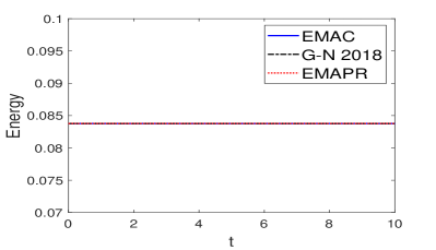
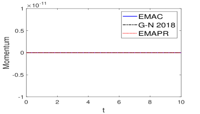
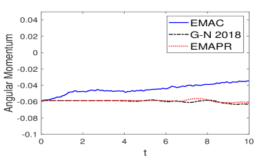
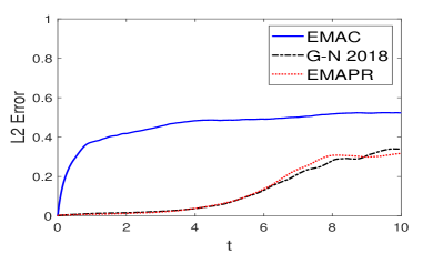
Figure 1. Example 2. Plots of kinetic energy, momentum, angular momentum and L2 errors by the Bernardi-Raugel element or Guzmán-Neilan element (G-N 2018) versus time.

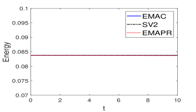
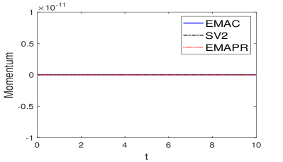
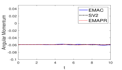
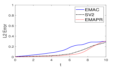
Figure 2. Example 2. Plots of kinetic energy, momentum, angular momentum and L2 errors by $P_{2}^{bubble}/P_{1}^{disc}$ or SV2 versus time.

5.3. Example 3: $Re$-semi-robustness test: the lattice vortex problem

In the final example, we consider the lattice vortex problem [42, 46] on $\Omega=\left(0,1\right)^{2}$, which is a benchmark to test the exponential growth rates (with respect to time) of the errors. In Section 4 we have shown that the Gronwall constant is independent of $\nu$. The exact velocity is set as $\boldsymbol{u}\left(t,\boldsymbol{x}\right)=\boldsymbol{u}^{0}\left(\boldsymbol{x}\right)\exp\left({-8\pi^{2}\nu t}\right)$ with $\boldsymbol{u}^{0}\left(\boldsymbol{x}\right)=\left(\sin\left(2\pi x\right)\sin\left(2\pi y\right),\cos\left(2\pi x\right)\cos\left(2\pi y\right)\right)^{\text{T}}$. With an appropriate $p$, $\boldsymbol{u}$ fulfills an exact unsteady NSE with $\boldsymbol{f}=\boldsymbol{0}$. To test the $Re$-semi-robustness, we choose a small $\nu$ and large $T$: $\nu=1\times 10^{-5}$ and $T=10$.

The methods (or elements) used in this example are the same as Section 5.2, except replacing the EMAC scheme with the classical skew-symmetric scheme (SKEW), which has been shown not to be $Re$-semi-robust with non-divergence-free elements [42, 46]. All the first order methods are run on the uniform $64\times 64$ triangular mesh. The $P_{2}^{bubble}/P_{1}^{disc}$ are tested on a non-uniform mesh with the size $h=0.03$, and the SV2 element is performed on the barycentric refinement of the same mesh. For our methods, we give the results for both $\alpha=0$ and $\alpha=1$. Note that from the theoretical analysis the value of $\alpha$ has an effect on the property of $Re$-semi-robustness. For the time discretizations, we use the Crank-Nicolson scheme with $\Delta t=0.001$. We linearize all the methods by replacing the first velocity in trilinear forms with some appropriate extrapolation of the previous step velocities.

Some results are shown in Figs. 3 and 4. One could find that the value of $\alpha$ does have an effect on the growth speed of the errors. For first order approximations, the methods (elements) proposed by Guzmán and Neilan in [27] give the best results, and our method with $\alpha=1$ gives very close performance in the final time. For second order approximations, our method admits the best performance. Except the SKEW formulation on non-divergence-free elements, all the methods below show a slower growth speed of the errors.

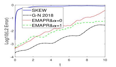
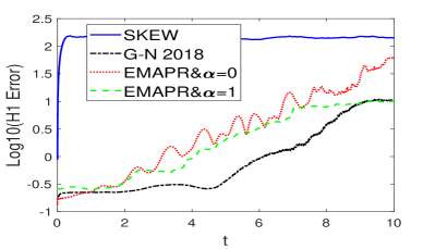
Figure 3. Example 3. Plots of L2 errors, H1 errors by the Bernardi-Raugel element or Guzmán-Neilan element versus time.

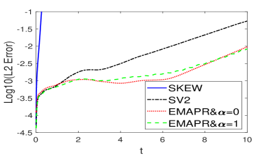
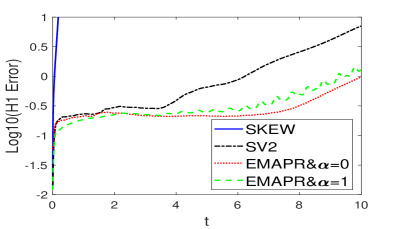
Figure 4. Example 3. Plots of L2 errors, H1 errors by $P_{2}^{bubble}/P_{1}^{disc}$ or SV2 versus time.

References

- [1] R.V. Abramov and A.J. Majda, Discrete approximations with additional conserved quantities: deterministic and statistical behavior, Methods Appl. Anal. 10 (2003), no. 2, 151–190.
- [2] Akio Arakawa, Computational design for long-term numerical integration of the equations of fluid motion: Two dimensional incompressible flow, Part I, J. Comput. Phys. 1 (1966), 119–143.
- [3] D. N. Arnold and J. Qin, Quadratic velocity/linear pressure Stokes elements, Advances in Computer Methods for Partial Differential Equations-VII, R. Vichnevetsky, D. Knight & G. Richter, eds., IMACS, New Brunswick, NJ (1992), 28–34.
- [4] Christine Bernardi and Genevieve Raugel, Analysis of some finite elements for the Stokes problem, Math. Comp. 44 (1985), no. 169, 71–79.
- [5] Daniele Boffi, Franco Brezzi, and Michel Fortin, Mixed finite element methods and applications, Springer Series in Computational Mathematics, vol. 44, Springer Berlin Heidelberg, 2013.
- [6] Susanne C. Brenner and L. Ridgway Scott, The mathematical theory of finite element methods, Texts in Applied Mathematics, vol. 15, Springer New York, New York, NY, 2008.
- [7] F. Brezzi, T. J. R. Hughes, L. D. Marini, and A. Masud, Mixed discontinuous Galerkin methods for Darcy flow, J. Sci. Comput. 22-23 (2005), no. 1-3, 119–145.
- [8] Erik Burman and Miguel A. Fernández, Continuous interior penalty finite element method for the time-dependent Navier-Stokes equations: space discretization and convergence, Numer. Math. 107 (2007), no. 1, 39–77.
- [9] Michael A. Case, Vincent J. Ervin, Alexander Linke, and Leo G. Rebholz, A connection between Scott-Vogelius and grad-div stabilized Taylor-Hood FE approximations of the Navier-Stokes equations, SIAM J. Numer. Anal. 49 (2011), no. 4, 1461–1481.
- [10] Sergey Charnyi, Timo Heister, Maxim A. Olshanskii, and Leo G. Rebholz, On conservation laws of Navier-Stokes Galerkin discretizations, J. Comput. Phys. 337 (2017), 289–308.
- [11] Sergey Charnyi, Timo Heister, Maxim A. Olshanskii, and Leo G. Rebholz, Efficient discretizations for the EMAC formulation of the incompressible Navier-Stokes equations, Appl. Numer. Math. 141 (2019), 220–233.
- [12] Snorre H. Christiansen and Kaibo Hu, Generalized finite element systems for smooth differential forms and Stokes’ problem, Numer. Math. 140 (2018), no. 2, 327–371.
- [13] Philippe G. Ciarlet, The finite element method for elliptic problems, Society for Industrial and Applied Mathematics, 2002.
- [14] Bernardo Cockburn, Guido Kanschat, and Dominik Schtzau, A note on discontinuous Galerkin divergence-free solutions of the Navier-Stokes equations, J. Sci. Comput. 31 (2007), no. 1-2, 61–73.
- [15] Javier de Frutos, Bosco García-Archilla, Volker John, and Julia Novo, Analysis of the grad-div stabilization for the time-dependent Navier-Stokes equations with inf-sup stable finite elements, Adv. Comput. Math. 44 (2018), no. 1, 195–225.
- [16] by same author, Error analysis of non inf-sup stable discretizations of the time-dependent Navier-Stokes equations with local projection stabilization, IMA J. Numer. Anal. 39 (2019), no. 4, 1747–1786.
- [17] Daniele Antonio Di Pietro and Alexandre Ern, Mathematical aspects of discontinuous Galerkin methods, Mathematiques et Applications, vol. 69, Springer Berlin Heidelberg, Berlin, Heidelberg, 2012.
- [18] John A. Evans and Thomas J. R. Hughes, Isogeometric divergence-conforming B-splines for the unsteady Navier-Stokes equations, J. Comput. Phys. 241 (2013), 141–167.
- [19] George J. Fix, Finite Element Models for Ocean Circulation Problems, SIAM J. Appl. Math. 29 (1975), no. 3, 371–387.
- [20] Bosco García-Archilla, Volker John, and Julia Novo, Symmetric pressure stabilization for equal-order finite element approximations to the time-dependent Navier-Stokes equations, IMA J. Numer. Anal. 41 (2021), no. 2, 1093–1129.
- [21] Nicolas R. Gauger, Alexander Linke, and Philipp W. Schroeder, On high-order pressure-robust space discretisations, their advantages for incompressible high Reynolds number generalised Beltrami flows and beyond, The SMAI journal of computational mathematics 5 (2019), 89–129.
- [22] V. Girault, R. H. Nochetto, and L. R. Scott, Max-norm estimates for Stokes and Navier-Stokes approximations in convex polyhedra, Numer. Math. 131 (2015), no. 4, 771–822.
- [23] Vivette Girault and Pierre-Arnaud Raviart, Finite element methods for Navier-Stokes equations, Springer Series in Computational Mathematics, vol. 5, Springer Berlin Heidelberg, Berlin, Heidelberg, 1986.
- [24] Johnny Guzmán and Michael Neilan, A family of nonconforming elements for the Brinkman problem, IMA J. Numer. Anal. 32 (2012), no. 4, 1484–1508.
- [25] by same author, Conforming and divergence-free Stokes elements on general triangular meshes, Math. Comp. 83 (2013), no. 285, 15–36.
- [26] Johnny Guzmán and Michael Neilan, Conforming and divergence-free Stokes elements in three dimensions, IMA J. Numer. Anal. 34 (2014), 1489–1508.
- [27] Johnny Guzmán and Michael Neilan, Inf-sup stable finite elements on barycentric refinements producing divergence–free approximations in arbitrary dimensions, SIAM J. Numer. Anal. 56 (2018), no. 5, 2826–2844.
- [28] Volker John, Finite element methods for incompressible flow problems, Springer, New York, 2016.
- [29] Volker John, Petr Knobloch, and Julia Novo, Finite elements for scalar convection-dominated equations and incompressible flow problems: a never ending story?, Comput. Visual Sci. 19 (2018), no. 5-6, 47–63.
- [30] Volker John, Alexander Linke, Christian Merdon, Michael Neilan, and Leo G. Rebholz, On the divergence constraint in mixed finite element methods for incompressible flows, SIAM Rev. 59 (2017), no. 3, 492–544.
- [31] Juho Könnö and Rolf Stenberg, -conforming finite elements for the Binkman problem, Math. Models Methods Appl. Sci. 21 (2011), no. 11, 2227–2248.
- [32] Philip L. Lederer, Pressure-robust discretizations for Navier-Stokes equations: Divergence-free reconstruction for Taylor-Hood elements and high order hybrid discontinuous Galerkin methods, Master’s thesis, Vienna Technical University, Vienna, 2016.
- [33] Philip L. Lederer, Christoph Lehrenfeld, and Joachim Schöberl, Hybrid discontinuous Galerkin methods with relaxed H(div)-conformity for incompressible flows. Part II, ESAIM: Math. Model. Numer. Anal. 53 (2019), no. 2, 503–522.
- [34] Philip L. Lederer, Alexander Linke, Christian Merdon, and Joachim Schöberl, Divergence-free reconstruction operators for pressure-robust Stokes discretizations with continuous pressure finite elements, SIAM J. Numer. Anal. 55 (2017), no. 3, 1291–1314.
- [35] Alexander Linke, On the role of the Helmholtz decomposition in mixed methods for incompressible flows and a new variational crime, Comput. Methods Appl. Mech. Engrg. 268 (2014), 782–800.
- [36] Alexander Linke, Gunar Matthies, and Lutz Tobiska, Robust arbitrary order mixed finite element methods for the incompressible Stokes equations with pressure independent velocity errors, ESAIM: Math. Model. Numer. Anal. 50 (2016), no. 1, 289–309.
- [37] Alexander Linke and Christian Merdon, Pressure-robustness and discrete Helmholtz projectors in mixed finite element methods for the incompressible Navier-Stokes equations, Comput. Methods Appl. Mech. Engrg. 311 (2016), 304–326.
- [38] Alexander Linke and Leo G. Rebholz, Pressure-induced locking in mixed methods for time-dependent Navier-Stokes equations, J. Comput. Phys. 388 (2019), 350–356.
- [39] Michael Neilan, Discrete and conforming smooth de Rham complexes in three dimensions, Math. Comp. 84 (2015), 2059–2081.
- [40] Michael Neilan and Baris Otus, Divergence-free Scott–Vogelius elements on curved domains, SIAM J. Numer. Anal. 59 (2021), no. 2, 1090–1116.
- [41] M. A. Olshanskii and A. Reusken, Grad-div stabilization for Stokes equations, Math. Comp. 73 (2004), 1699–1718.
- [42] Maxim A. Olshanskii and Leo G. Rebholz, Longer time accuracy for incompressible Navier-Stokes simulations with the EMAC formulation, Comput. Methods Appl. Mech. Engrg. 372 (2020), 113369.
- [43] A. Palha and M. Gerritsma, A mass, energy, enstrophy and vorticity conserving (MEEVC) mimetic spectral element discretization for the 2D incompressible Navier-Stokes equations, J. Comput. Phys. 328 (2017), 200–220.
- [44] Leo G. Rebholz, An energy- and helicity-conserving finite element scheme for the Navier-Stokes equations, SIAM J. Numer. Anal. 45 (2007), no. 4, 1622–1638.
- [45] Sander Rhebergen and Garth N. Wells, An embedded-hybridized discontinuous Galerkin finite element method for the Stokes equations, Comput. Methods Appl. Mech. Engrg. 358 (2020), 112619.
- [46] Philipp W. Schroeder, Christoph Lehrenfeld, Alexander Linke, and Gert Lube, Towards computable flows and robust estimates for inf-sup stable FEM applied to the time-dependent incompressible Navier-Stokes equations, SeMA 75 (2018), no. 4, 629–653.
- [47] Junping Wang, Xiaoshen Wang, and Xiu Ye, Finite element methods for the Navier-Stokes equations by elements, J. Comput. Math. 26 (2008), 410–436.
- [48] Junping Wang and Xiu Ye, New finite element methods in computational fluid dynamics by elements, SIAM J. Numer. Anal. 45 (2007), no. 3, 1269–1286.
- [49] Shangyou Zhang, A new family of stable mixed finite elements for the 3D Stokes equations, Math. Comp. 74 (2005), no. 250, 543–554.