Deterministic cellular automata resembling diffusion

1 Introduction

The phenomenon of diffusion is very common in various natural, technological, economic and social systems. What is usually understood by it is the movement of particles (or ideas, biological organisms, people, price values, etc.) from a region of higher concentration to a region of lower concentration. At the microscopic level, the driver of the diffusion is the random walk or Brownian motion of individual particles. When diffusion is simulated in computer software, for example, in order to numerically investigate a model of a natural phenomenon, random walks must be simulated using pseudo-random number generator, consuming significant CPU resources. Alternatively, diffusion can be modeled and studied using partial differential equations, such as the heat equation or Fick’s laws of diffusion. Such equations must be first discretized in order to solve them numerically on digital computers.

If the objective is to construct a computer model which exhibits movement form higher to lower concentrations, it would be obviously best to avoid using random numbers and differential equations, devising the model from the beginning in such a way that it operates in the space of binary strings. All what is then needed is to find the right dynamical system “living” in such a space and resembling diffusion to the extent it is possible. Cellular automata seem to be ideally suited for this purpose, since they are fully discrete analogs of partial differential equations, with discrete space, time, and state variables.

Our goal in this paper is, therefore, to search for binary cellular automata which share some features with broadly understood diffusion processes, and to find out how well they resemble the actual diffusion (if alt all).

In order to have some sort of benchmark to compare with, let us consider a model of “real” diffusion constructed as follows. Consider one dimensional lattice with lattice sites being either empty (state 0) or occupied by a single particle (state 1). All particles simultaneously and independently of each other decide whether to move to the left or to the right, with the same probability 0.5 in either direction. We then simultaneously move every particle to the desired position if it is empty, otherwise the particle stays in the same place. If two particles want to move to the same empty spot, only one of them, randomly selected, is allowed to do so. This process, which constitutes a single time step, is then repeated for as many time steps as desired.

Figure 1 illustrates this process for 40 particles initially occupying a block of 40 sites in the middle of the lattice of 250 sites. Consecutive iterations are shown every 10 steps as individual rows. Black squares represent particles, empty spaces are shown in white color.

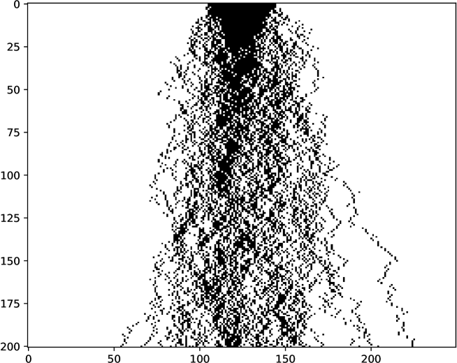
Figure 1: Spatiotemporal pattern of random diffusion on one dimensional lattice of 250 sites. The initial condition is a solid block of 40 particles. Every 10th time step is shown, so that the numbers on the vertical axis correspond to the actual time divided by 10.

We can see that with the passage of time the particles occupy wider and wider region. This is analogous to the behaviour of a gas which, if released in a small region of a container, will eventually spread over the entire container.

Three features of the above process are crucial: (i) the “gas” of particles expands in space, (ii) the total number of particles is conserved and (iii) the arrangement of particles appears more and more disordered (spatial entropy increases). While our ultimate goal is to find (or construct) CA rules satisfying all three conditions, in this paper we will pursue a more modest goal, namely we will investigate binary cellular automata satisfying the first two conditions only.

2 Basic definitions

Let $f:\{0,1\}^{n}\to\{0,1\}$ be called a local function or rule of cellular automaton, where $n>0$. We will sometimes refer to it as $n$-input rule. Let $l$ and $r$ be two positive integers called, respectively, left radius and right radius such that $l+r+1=n$. For a given local function $f$, we define the global function $F:\{0,1\}^{\mathbbm{Z}}\to\{0,1\}^{\mathbbm{Z}}$ such that for all $x\in\{0,1\}$ we have

$$[F(x)]_{i}=f(x_{i-l},x_{i-l+1},\ldots,x_{i+r}).$$

It is customary to refer to CA rules by their Wolfram number [9], defined as

$$W(f)=\sum_{(x_{1},x_{2},\ldots x_{n})\in\{0,1\}^{n}}2^{2^{n-1}x_{1}+2^{n-2}x_{2}+\ldots 2^{0}x_{n}}.$$

When discussing family of specific CA rules it is usually convenient to divide them into equivalence classes of rules having similar properties [9, 1]. These equivalence classes are defined with respect to the group generated by the operators of reflection and conjugation denoted, respectively by $R$ and $C$, and defined on the set of all one-dimensional binary $n$-input CA rules $f$ by

$$R\,f(x_{1},x_{2},\ldots,x_{n}) =f(x_{n},x_{n-1},\ldots,x_{1}),$$

$$C\,f(x_{1},x_{2},\ldots,x_{n}) =f(1-x_{1},1-x_{2},\ldots,1-x_{n}).$$

In some cases, equivalence classes generated by the operator $R$ alone are more appropriate, and we will discuss this later in the paper.

A one-dimensional $n$-input CA rule $f$ is number-conserving if, for all $L\geq n$ and all $(x_{1},x_{2},\ldots,x_{L})\in\{0,1\}^{L}$ it satisfies

$$\sum_{i=0}^{L-1}f(x_{i},x_{i+1},\ldots,x_{i+n-1})=\sum_{i=0}^{L-1}x_{i}$$ (1)

where all indices are taken modulo $L$.

Property of being number-conserving is decidable and easily checked, using the well known method described in [3]. These rules have been exnensively studied in the past [6, 5, 4, 8, 7]. It is well known that there exist

• 5 number conserving rules with 3 inputs, rules 184, 226, 170, 240 and 204, although the local functions of the last three effectively depend on 1 input only;

• 22 number conserving rules with 4 inputs, although 8 of them depend effectively on 3 or less inputs only.

• 428 number conserving rules with 5 inputs,

Decompression ratio for cellular automata

As remarked in the introduction, we will be searching for rules which behave like “expanding gas” and which conserve the number of particles. The second condition will obviously be satisfied by number conserving rules, thus we will restrict our attention to such rules from now on. As for the first condition, we need to quantify the notion of “expansion”.

Let $x\in{\{0,1\}}^{\mathbbm{Z}}$ be a bi-infinite binary sequence, to be called configuration. The set of indices $i$ corresponding to nonzero values of $x_{i}$ will be called support of $x$,

$$\mathop{\mathrm{supp}}x=\{i\in{\mathbbm{Z}}:x_{i}\neq 0\}.$$

If $\mathop{\mathrm{supp}}x$ is finite, then we can define diameter of $x$,

$$\mathop{\mathrm{diam}}(x)=\max\mathop{\mathrm{supp}}x-\min\mathop{\mathrm{supp}}x+1$$

For $x$ with finite support, we define density of support as

$$\rho(x)=\frac{\sum_{i\in{\mathbbm{Z}}}x_{i}}{\mathop{\mathrm{diam}}(x)}$$

Now let us suppose that $F$ is the global function of some cellular automaton, so that $F^{k}(x)$ denotes the configuration obtained by iterating $F$ $k$ times. For $x$ with finite support and for a number-conserving $F$,

$$\sum_{i\in{\mathbbm{Z}}}x_{i}=\sum_{i\in{\mathbbm{Z}}}[F^{k}(x)]_{i}$$

for any $k\in{\mathbbm{N}}$.

Define decompression ratio for a given cellular automaton $F$ and a configuration $x$ as

$$\psi_{F}(x)=\lim_{k\to\infty}\frac{\mathop{\mathrm{diam}}\left(F^{k}(x)\right)}{\mathop{\mathrm{diam}}(x)}.$$

Figure 2 shows an example calculation of the decompression ratio in a concrete situation. In this example the the decompression ratio reaches certain limit after a finite number of iterations and stays constant thereafter. As we shall see, this will be a common feature in number-conserving CA.

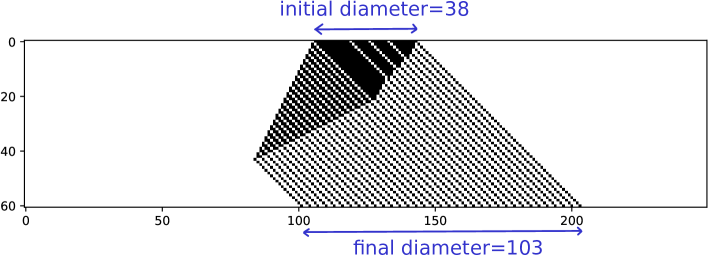
Figure 2: Calculations of the decompression ratio for a sample initial configuration and 4-input rule 60200. Here $\psi_{F}(x)=\frac{103}{38}=\approx 2.71$

Since the decompression ratio for a given rule depends on the initial configuration, we need to average it out over all configurations. We will achieve this by considering the set of all configurations which have a given fixed diameter and a given number of ones. More formally, let $d>2$, $2\leq n\leq d$ and and let $D_{d,n}$ be the set of all configurations $x\in{\{0,1\}}^{\mathbbm{Z}}$ with support starting at the origin, such that they have exactly $m$ 1’s and $\mathop{\mathrm{diam}}x=d$. Since the number of binary strings of length $a$ having exactly $b$ 1’s is equal to $\binom{a}{b}$, it immediately follows that

$$\mathop{\mathrm{card}}D_{d,n}=\binom{d-2}{n-2}.$$

Then we define expected decompression ratio as

$$\psi_{d,p,F}=\frac{\sum_{x\in D_{d,n}}\psi_{F}(x)}{\mathop{\mathrm{card}}D_{d,n}},$$

where $p=n/d$ represents the density of support of configurations in $D_{d,n}$. The expected decompression ratio can still possibly depend on the diameter $d$, thus we will define

$$\psi_{p,F}=\lim_{d\to\infty}\psi_{d,p,F}.$$

Finally, since $p\in[0,1]$, we can average the above over $p$, obtaining a single number, to be called a rule decompression ratio, defined as

$$\psi_{F}=\frac{\int_{0}^{1}\psi_{p,F}\,dp}{\int_{0}^{1}dp}=\int_{0}^{1}\psi_{p,F}\,dp.$$

Computing $\psi_{F}$ for a given CA is not easy, although we will see later that it can be accomplished in some cases. We can, however, compute its approximate value as follows.

For a given $p\in[0,1]$ and $d$, we set $n=pd$ and randomly generate a binary string of length $d-2$ with exactly $n-2$ ones, selecting it randomly with uniform probability from the set of all such strings. We add 1 in front and at the end of this string, obtaining a string with $n$ ones having diameter $d$. We then add a number of zeros in front and end obtaining a finite configuration of length $M$. We then iterate rule $F$ for a sufficient number of time steps so that the diameter expands to its limiting value and compute $\psi_{d,p,F}$. This is repeated for values of $p$ ranging from 0 to 1, with small increments. We then plot the decompression ratio versus $p$. This, if $d$ is sufficiently large, approximates the graph of $\psi_{p,F}$ vs. $p$.

Figure 3 shows an example of such a plot for rule 60200.

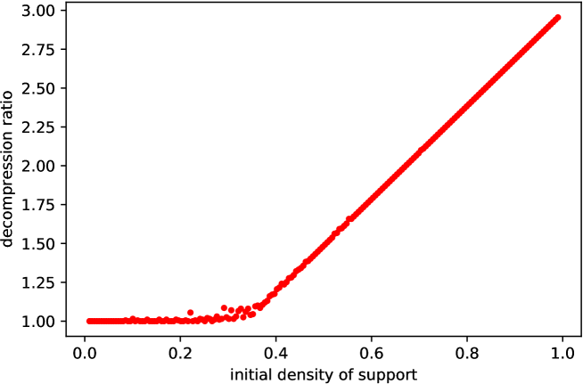
Figure 3: Decompression ratio $\psi_{d,p,F}$ vs. initial density of support $p$ for rule 60200. Graph obtained numerically by generating random samples of configurations with support diameter $d=200$ and iterating rule 60200 until diameter stops changing.

From this graph, we could conjecture that for rule 60200 the decompression factor is

$$\psi_{p,F}=\begin{cases}1&\mbox{if }p<1/3,\\ 3p&\mbox{otherwise.}\end{cases}$$

With the above, we can now compute the rule decompression ratio for rule 60200,

$$\psi_{F}=\int_{0}^{1/3}dp+\int_{1/3}^{1}3p\,dp=\frac{1}{3}+\frac{4}{3}=\frac{5}{3}.$$

For other number conserving rules the rule decompression ratio can be obtained in a similar way. We will carry out this procedure for rules with 3, 4 and 5 inputs in order to fin the “best” rule among them, that is, the rule which features the largest decompression ratio.

3 Rules with three inputs

Among the number conserving rules with three inputs, three are trivial. These are rules 170 and 240 (shifts) as well as rule 204 (identity). All three preserve diameters of configurations with finite support, thus for them $\psi_{F}=1$.

Rule 184 (and its reflected version rule 226) is more interesting. Due to the nature of rule 184, for a given $x\in D_{d,n}$, the diameter of $F^{k}(x)$ is non-decreasing with $k$, and reaches the limiting value after the final number of steps. Define, therefore, the final diameter as

$$\lim_{k\to\infty}\mathop{\mathrm{diam}}F^{k}(x).$$

For a given $x\in D_{d,n}$, the final diameter is bounded. One can show the following.

Proposition 1.

Let $d>2$, $2\leq n\leq d$. For rule 184, for every $x\in D_{d,n}$, the final diameter of $x$ is bounded by

$$d_{min}\leq\lim_{k\to\infty}\mathop{\mathrm{diam}}F^{k}(x)\leq d_{max},$$ (2)

where

$$d_{min}=\begin{cases}d&\mbox{if }2\leq n\leq d/2,\\ 2n-1&\mbox{otherwise,}\end{cases}$$ (3)

and

$$d_{max}=\begin{cases}d+n-2&\mbox{if }n<d,\\ 2d-1&\mbox{if $n=d$.}\end{cases}$$ (4)

Proof. Let us consider $d_{max}$ first. Rule 184 can be viewed as particle system, where each particle (site in state 1) will move to the right in the next time step if its right neighbour is empty [2]. Since the rightmost particle has always 0 as its right neighbour, it will always move. The rightmost particle, on the other hand, can be stopped, and if it is stopped, diameter grows (because the rightmost one moves at the same time). Therefore, in order to maximized the final diameter, we need to put all inside particles grouped in a solid block on the left, as shown in Figure 4a. If we do it, the leftmost site will be stopped for $n-2$ steps, so the diameter will increase by $n-2$, reaching final value $d+n-2$. The only exception to this is the case when $n=d$, as shown in Figure 4b. In this case, the leftmost site is stopped for one more extra step, so that the final diameter is $d+n-2+1=2d-1$. This yields the upper bound given in eq. (4).

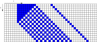
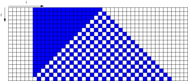
(a)  (b)

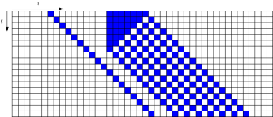
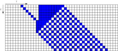
(c)  (d)

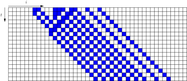
(e)(f)

Figure 4: Spatiotemporal patterns for rule 184 used in the proof of Proposition 1.

In order to achieve the minimal final diameter, we need to group inside particles as far to the right as possible, as shown in Figures 4c and 4d. If $n\leq d/2$, the leftmost site is never stopped, so that the diameter does not change at all and is always equal to $d$, as in Figure 4c. If $n>d/2$, the final pattern is of the form $101010\ldots 10$, that is, it consists of $n$ repeated pairs $10$, as shown in in Figure 4d. Diameter of this configuration is $2n-1$. This yields the lower bound given in eq. (3).

Proposition 2.

Let $d>2$, $2\leq n\leq d$. The number of elements of $D_{d,n}$ having the final diameter $d_{f}$, to be denoted as $N(d_{f})$, is given by

$$N(d_{f})=\begin{cases}\displaystyle\binom{d-2}{d_{f}-n}-\binom{d-2}{d_{f}-n+1}&\mbox{if }d_{f}\neq 2n-1,\\[15.00002pt] \displaystyle\binom{d-2}{n-2}-\binom{d-2}{n}&\mbox{if }d_{f}=2n-1.\end{cases}$$ (5)

Proof. We will start with the case $d_{f}=2n-1$. As we already know from the proof of the previous proposition, $d_{f}=2n-1$ means that the final pattern consists of alternating 1’s and 0’s, as in Figures  4d and  4e. In order to reach this configuration, we must make sure that in the initial configuration any cluster of zeros disappears before the final configuration is reached. Let us define the rightmost substring of a given string $s$ as the substring of $s$ which ends at the end of $s$.

The final configuration $101010\ldots 1$ will be obtained if any rightmost substring of the support of the initial configuration has no more 0’s than 1’s. The number of binary strings of length $d$ staring and ending with 1, having exactly $n$ 1’s and having the property that any rightmost substring of it has no more 0’s than 1’s is equal to

$$\binom{d-2}{n-2}-\binom{d-2}{n},$$

exactly as claimed in eq. (5).

When $d_{f}\neq 2n-1$, the final configuration will not be $101010\ldots 1$, but will include some extra 0’s, as in the example in Figure 4f. The number of such extra zeros is $\epsilon=d_{f}-(2n-1)$. Final configuration with $\epsilon$ extra zeros is obtained when among the rightmost substrings of the support of the initial configuration the maximal excess of 0’s over 1’s is $\epsilon$. The number of binary strings of length $d$ staring and ending with 1, having exactly $n$ 1’s and having the property that among the rightmost substrings of each of of them the maximal excess of 0’s over 1’s equals $\epsilon$ is given by

$$\binom{d-2}{\epsilon+n-1}-\binom{d-2}{\epsilon+n}=\binom{d-2}{d_{f}-n}-\binom{d-2}{d_{f}-n+1},$$

again in agreement with eq. (5). $\Box$

We can now compute the decompression ratio for rule 184 as

$$\psi_{d,p,F}=\frac{\sum_{d_{f}=d_{min}}^{d_{max}}\frac{d_{f}}{d}N(d_{f})}{\sum_{d_{f}=d_{min}}^{d_{max}}N(d_{f})}.$$

The denominator of the above, as we already remarked, equals to $\binom{d-2}{n-2}$, thus we obtain

$$\psi_{d,p,F}=\frac{1}{d}{\binom{d-2}{n-2}}^{-1}\sum_{d_{f}=d_{min}}^{d_{max}}d_{f}N(d_{f}),$$ (6)

where $n=pd$ is rounded to the nearest integer, $N(d_{f})$ is given by eq. (5), and $d_{min}$, $d_{max}$ are given by eqs. (3–4).

Although it does not seem to be possible to compute the closed form of the sum in the above formula, numerical plot of the decompression ratio can easily be produced. Figure 5 shows the plot of $\psi_{d,p,F}$ as a function of $p$ for two different values of $d$. One can see that as $d$ increases, the graph develops a “sharp corner” at $p=1/2$.

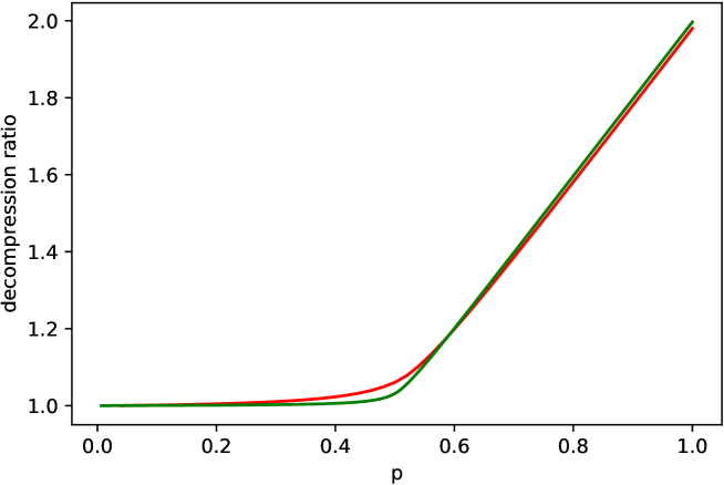
Figure 5: Graph of the decompression ratio $\psi_{d,p,F}$ as a function of $p$ for rule 184, obtained from eq. (6) using $d=50$ (red) and $d=300$ (green).

Indeed, our numerical investigations of the behaviour of $\psi_{d,p,F}$ for large $d$ indicate that for rule 184,

$$\psi_{p,F}=\lim_{d\to\infty}\psi_{d,p,F}=\begin{cases}1&\mbox{if }p<1/2,\\ 2p&\mbox{otherwise.}\end{cases}$$ (7)

This yields $\psi_{F}=\int_{0}^{1}\psi_{p,F}\,dp=1.25$.

4 Four input rules

In section 2 we remarked that there are 22 4-input rules. Some of these are not really 4-input, but they effectively depend on 3 inputs (or less), and as such they do not need to be considered because they were discussed in the previous section. What is left is 14 rules falling into 7 equivalence classes with respect to spatial reflection, $\{43944,65026\}$, $\{48268,63544\}$, $\{48770,60200\}$, $\{49024,59946\}$, $\{51448,62660\}$, $\{52930,58336\}$, and $\{56528,57580\}$. It is obvious that each pair has the same rule decompression ratio and the same graph of $\psi_{d,p,f}$ vs. $p$, thus only one of each needs to be considered.

One should remark at this point that it is customary in CA research to divide rules into equivalence classes with respect to the group generated by spatial reflection and conjugation. For the 14 aforementioned 4-input rules these equivalence classes would be $\{48770,60200\}$, $\{43944,49024$, $59946,65026\}$, $\{48268,52930,58336,63544\}$, and $\{51448,56528,57580,62660\}$. However, since our definition of the decompression ratio is not symmetric with respect to interchange of 0’s and 1’s, rules belonging to the same equivalence class of this type may have different graphs of $\psi_{d,p,F}$ and different $\psi_{F}$. This classification, therefore, is not very useful for our purposes.

We investigated the behaviour of of $\psi_{d,p,F}$ numerically for all representative 4-input rules. It turns out that for rules $\{51448,62660\}$ the diameter grows unbounded, and thus we say that $\psi_{F}=\infty$ for these two rules. The remaining rules have finite $\psi_{F}$, and their graph of $\psi_{d,p,F}$ vs. $p$ is one of four types shown in Figure 6.

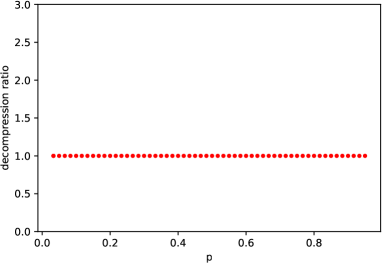
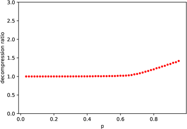
(a)    (b)

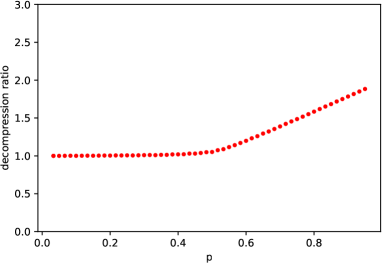
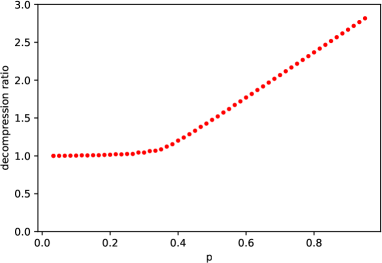
(c)     (d)

Figure 6: Four types of graphs of numerically computed decompression ratio $\psi_{d,p,F}$ as a function of $p$ for 4-input rules. Graphs obtained by random sampling of 100 initial configurations for each $p$ using initial diameter $d=60$. Representative graphs are shown: they vary sightly between rules, but the differences disappear as $d\to\infty$.

We found a rather remarkable fact, namely, for $d\to\infty$, all finite decompression ratios $\psi_{p,F}$ appear to assume the same functional form,

$$\psi_{p,F}=\lim_{d\to\infty}\psi_{d,p,F}=\begin{cases}1&\mbox{if }p<p_{c},\\ p/p_{c}&\mbox{otherwise,}\end{cases}$$ (8)

where $p_{c}$ takes one of the values $1/3$, $1/2$, $2/3$ or $1$. The graph types as well as $p_{c}$ for all 4-input rules are shown in Table 1 (for completeness, 3-input rules are included as well).

Using eq. (8) it is now straightforward to compute the rule decompression ratio,

$$\psi_{F}=\int_{0}^{1}\psi_{p,F}\,dp=\frac{1+p_{c}^{2}}{2p_{c}},$$ (9)

and the relevant values are shown in the last column of Table 1.

	$W(f)$	graph type	$p_{c}$	$\psi_{F}$	decimal value of $\psi_{F}$
3-input	170,240	a	1	1	1.0
	204	a	1	1	1.0
	184,226	c	1/2	5/4	1.25
4-input	43944, 65026	d	1/3	5/3	1.666…
	48268, 63544	c	1/2	5/4	1.25
	48770, 60200	d	1/3	5/3	1.666…
	49024, 59946	b	2/3	13/12	1.0833…
	51448, 62660	n/a	n/a	$\infty$	n/a
	52930, 58336	d	1/3	5/3	1.666…
	56528, 57580	a	1	1	1.0

Table 1: Estimated rule decompression ratio for 3-input and 4-input rules.

From the graphs and table we can conclude that the highest finite rule decompression ratio obtainable for 4-input rules is $5/3$. This is are only slightly better than the value for rule 184. None of the 4-input rules are particularly good for decompressing initial configurations with small densities: in fact, they do not decompress at all if the density of support of the initial configuration is less than $1/3$. When the density increases beyond the critical value $p_{c}$, the decompression ratio grows linearly, reaching the maximum value for strings consisting of only 1’s.

Rule 51448, for which the decompression ratio is infinite, indeed expands diameters without any bound, yet it is not performing “spreading” of particles in a particularly satisfactory way. In fact, as we can see in Figure 7, it performs consolidation of some particles on the right, which then move as a solid block to the right while other particles remain in place. This rule does not increase disorder, or, in other words, does not increase entropy in the same way as diffusion proces illustrated in Figure 1.

Figure 7: Example of a spatiotemporal pattern for rule 51448 demonstrating unbounded growth of the diameter.

5 Five input rules

There exist 428 number conserving CA rules with 5 inputs. They can be divided into 215 equivalence classes with respect to spatial reflection, or into 129 classes with respect to reflection and conjugation. In order to survey the types of behaviour which is possible in 5-input rules and keep their number manageable, we decided to use representatives of the later 129 classes. The representative chosen for each equivalence class is the rule with with minimal Wolfram number. One should keep in mind, however, as remarked in the previous section, that such a representative may not necessarily have the same decompression ratio as other members of the same class. Out of the aforementioned 129 rules there are 13 which effectively depend on 4 inputs or less, and these are eliminated. This leaves 116 rules.

We found that there are three types of behaviour of $\psi_{d,p,F}$ as a function of $p$:

1. rules exhibiting infinite decompression ratio. We found 5 rules of this type.

2. rules with “hockey-stick” type graphs of the form of eq. (8). There are 85 rules of this type.

3. 26 rules with “irregular” decompression graphs, as shown in examples of Fig. 8.

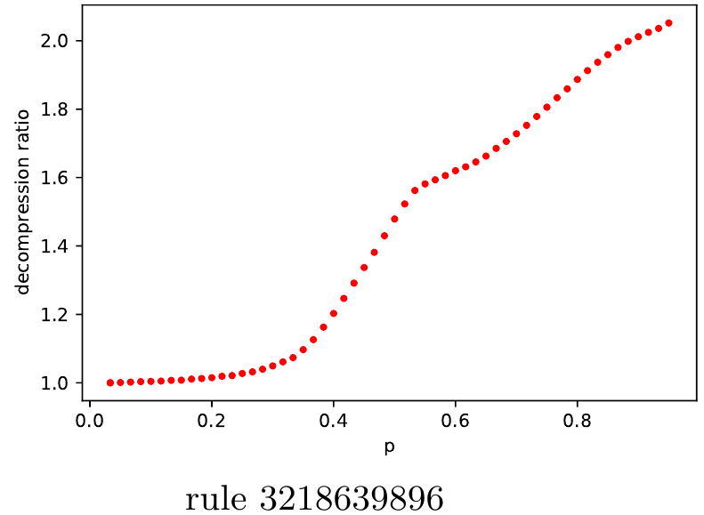
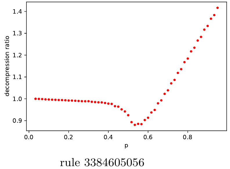
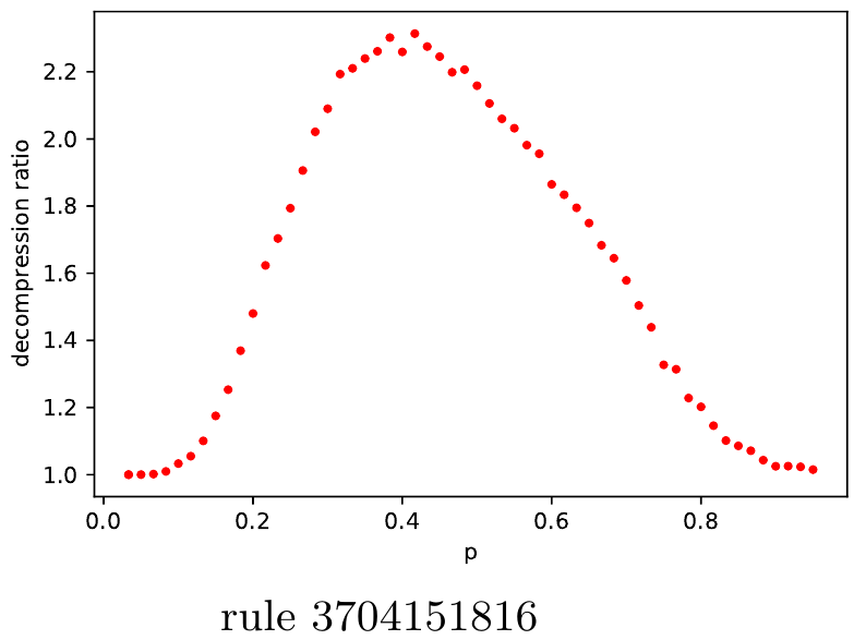
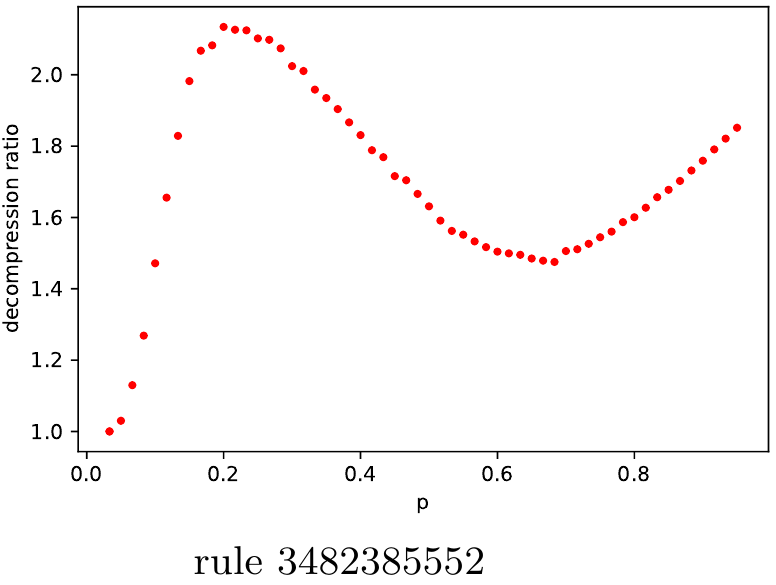
Figure 8: Examples of 5-input rules with “irregular” decompression graphs.

Regarding the second type, the smallest value of $p_{c}$ we found is $p_{c}=1/4$. This, together with the results for rules with 3 and 4 inputs presented earlier, suggests the following conjecture.

Conjecture 1.

If a CA rule with $n$ inputs exhibits decompression ratio of the form of eq. (8), then

$$p_{c}\geq\frac{1}{n-1}.$$

We have no proof of the above, but some intuition can be offered. A given site can interact with $n-1$ other sites, due to the nature of the local function. The expansion of a pattern can only happen if close particles are repelling each other. Obviously, they can repell each other only if they are located within the range of interaction. If we have on average less than one particle per $n-1$ sites, they will not be able to interact, thus there will be no expansion, and $\phi_{p,F}$ will remain 1. This means that $p_{c}=1/(1-n)$ is the lowest threshold for the transition from the non-expanding to the expanding regime.

As for the last type, rules with “irregular” decompression graphs, these often are very slowly converging. In fact, some rules which we now consider type 2, in our initial experiments were classified as type 3. Only when we increased the diameter and the number of iterations they assumed the shape of the “hockey stick”. For this reason, it is quite possible that future more extensive numerical experiments may reveal that some of type 3 rules still exhibit the form of eq. (8).

6 Conclusions

We found that deterministic number conserving cellular automata rules exhibit mostly very limited resemblance to diffusion. Although they expand the patterns with finite support, the vast majority of them spread only patterns with high density, and not patterns with low density. It is rather remarkable that the large percentage of them exhibits decompression ratio graphs in the form of of eq. (8). The existence of the transition at $p=p_{c}$ and the fact that such transition occurs in a large number of rules needs to be investigated further.

There exist, however, a small number of rules which exhibit infinite decompression ratio. These expand diameters of patterns with finite support, including even patterns with low density. Their behavior, however, differs from the random diffusion because they only increase the diameter without increasing the spatial entropy of the configuration. In order to construct a CA rule which is a better model of random diffusion one will likely need more than two states, with some states acting like pseudo-random generators, while others contributing to the increase of the diameter. Work in this direction is ongoing, and results will be reported elsewhere.

References

- [1] N. Boccara. Transformations of one-dimensional cellular automaton rules by translation-invariant local surjective mappings. Physica D, 68:416–426, 1993.
- [2] N. Boccara and H. Fukś. Cellular automaton rules conserving the number of active sites. J. Phys. A: Math. Gen., 31:6007–6018, 1998.
- [3] N. Boccara and H. Fukś. Number-conserving cellular automaton rules. Fundamenta Informaticae, 52:1–13, 2002.
- [4] B. Durand, E. Formenti, and Z. Róka. Number-conserving cellular automata I: decidability. Theoretical Computer Science, 299:523–535, 2003.
- [5] E. Formenti and A. Grange. Number conserving cellular automata II: dynamics. Theoretical Computer Science, 304:269–290, 2003.
- [6] T. Hattori and S. Takesue. Additive conserved quantities in discrete-time lattice dynamical systems. Physica D, 49:295–322, 1991.
- [7] A. Moreira. Universality and decidability of number-conserving cellular automata. Theor. Comput. Sci., 292:711–721, 2003.
- [8] M. Pivato. Conservation laws in cellular automata. Nonlinearity, 15:1781–1793, 2002.
- [9] S. Wolfram. Cellular Automata and Complexity: Collected Papers. Addison-Wesley, Reading, Mass., 1994.